23
Clean in Place Rinse Water Validation Using a LONESTAR TM Portable Analyzer Detection of common water rinse odor contaminants Contact us www.owlstonenanotech.com
Clean in Place Rinse Water Validation Using a LONESTARTM Portable
Analyzer Detection of common water rinse odor contaminants
Contact us
www.owlstonenanotech.com
2 | P a g e
Contents
Summary ......................................................................................................................................... 3
The LONESTARTM Portable Analyzer ............................................................................................... 4
Sample preparation ........................................................................................................................ 5
Water background ...................................................................................................................... 5
Water background + other trace solvents .................................................................................. 5
Experimental set up ........................................................................................................................ 5
Results – Water blanks vs. Analyte Spectra .................................................................................... 6
Water background - Standard humidity ..................................................................................... 6
Ethyl isovalerate 0.05 ppm ..................................................................................................... 6
Ionone (alpha) 10 ppb ............................................................................................................. 6
Lactones (gamma + deca) 1 ppm ............................................................................................ 7
Methyl anthranilate 0.02 ppm ................................................................................................ 8
Allyl hexanoate 3 ppm ............................................................................................................ 8
cis-3-hexenyl acetate 2 ppm ................................................................................................... 9
Indole 0.3 ppm ...................................................................................................................... 10
Iso amyl acetate 5.5 ppm ...................................................................................................... 11
Methyl 2-methylbutyrate 5 ppm .......................................................................................... 11
Water background - Detection at lower humidities ................................................................. 12
Anisyl acetate 0.01 ppm, 4.7% RH ........................................................................................ 12
Ethyl propionate 0.045ppm, 4.8% RH ................................................................................... 13
Hexyl acetate 0.04 ppm, 5% RH ............................................................................................ 13
Benzyl acetate 270 ppb, 5% RH ............................................................................................ 14
Water background + Trace solvents ......................................................................................... 15
2-isopropyl-4-methylthiazole 0.5 ppm, with trace propylene glycol ................................... 15
2-isopropyl-4-methylthiazole 0.5 ppm, with trace ethanol.................................................. 15
Appendix A: FAIMS Technology at a Glance ................................................................................. 16
Sample preparation and introduction ...................................................................................... 16
Carrier Gas ................................................................................................................................ 17
Ionisation Source ...................................................................................................................... 17
Mobility ..................................................................................................................................... 20
Detection and Identification ..................................................................................................... 21

3 | P a g e
Summary
Processing plants in the food, beverage, pharmaceutical and cosmetics industries commonly use the Clean in Place (CIP) method to sanitize tanks, piping, filters, pumps etc. between production batches. CIP is also often used to sanitize groundwater source boreholes at mineral water bottling facilities. Cleaning solution and rinse water are circulated around the system automatically, preventing time consuming manual processes such as disassembly. The validation of CIP processes is vital in all sectors and direct, rapid and accurate monitoring of the composition of CIP process rinse water offers significant cost savings based on:
Reduced water usage Reduced cleaning chemical consumption Reduced disposal costs for wastewater Reduced cycle times - increased process efficiency Increased available process time
This paper demonstrates the ability of the LONESTARTM portable analyzer to provide real time CIP rinse water validation. Table 1 shows a selection of water rinse contaminating odor compounds relevant to the beverage industry that were found to be detectable in a water background with LONESTARTM. The quoted concentrations are for the samples tested and do not represent lower limits of detection for the compounds. In many cases, further work and method optimisation will allow detection at considerably lower concentrations.
Table 1 CIP water rinse contaminants and odor compounds detectable using Lonestar
Compound Concentration Compound Concentration
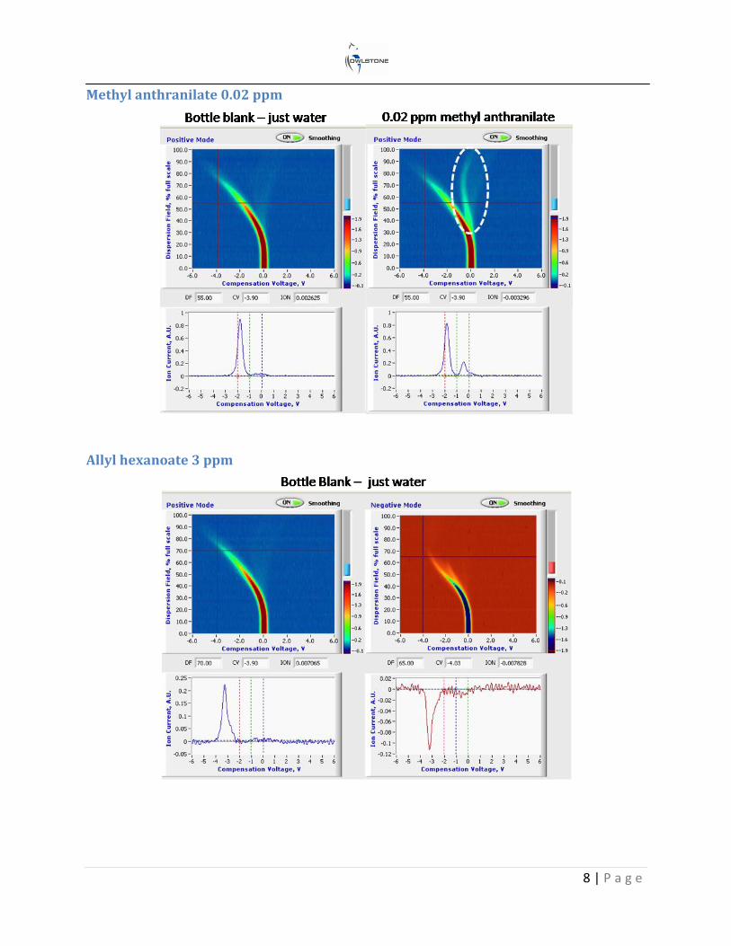
Ethyl isovalerate 0.05 ppm Allyl hexanoate 3 ppm
cis-3-hexenyl acetate 2 ppm Indole 0.3 ppm
Ionone (alpha) 0.01 ppm 2-isopropyl-4-methylthiazole
0.5 ppm
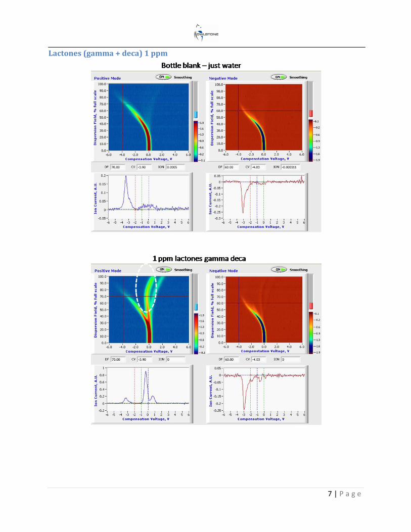
Lactones (gamma, deca)
1 ppm Methyl 2-methyl butyrate
5 ppm
Methyl anthranilate 0.02 ppm Hexyl acetate 0.04 ppm
Benzyl acetate 0.27 ppm Anisyl acetate 0.01 ppm
Ethyl propionate 0.045 ppm Isoamyl acetate 5.5 ppm

4 | P a g e
The LONESTARTM Portable Analyzer
The LONESTAR is an analytically powerful, portable chemical analyzer that can be operated by non-specialists. Incorporating Owlstone’s proprietary FAIMS technology (see Appendix A), the instrument combines high sensitivity and selectivity. New methods can be developed using Owlstone’s EasySpec software, making the LONESTAR suitable for a broad range of applications in process based industries.
Figure 1 LONESTAR connection figures

5 | P a g e
Sample preparation
Water background
To simulate the sampling conditions required for CIP rinse water validation, an aqueous solution of known concentration was prepared for each compound (see Table 1).
Water background + other trace solvents
CIP rinse water may to also contain traces of other solvents. The effect of trace ethanol and propylene glycol on the detection of 2-isopropyl-4-methylthiazole in a water background was also tested. Aqueous solutions of 2-isopropyl-4-methylthiazole of known concentration were prepared and spiked with either ethanol or propylene glycol.
Experimental set up
The response of the Lonestar unit to the simulated rinse water samples was investigated using the headspace sampling technique. A total flow of 1.8 l min-1 was passed through the headspace of a cleaned glass bottle containing a 20 ml of water + analyte. Control experiments were also performed in which the headspaces of bottles containing only purified water were sampled to gauge the blank response from the water background. The system pressure was maintained at 1 bar and the sample line between the headspace and the Lonestar was heated to prevent any condensation of the analyte. The Detection of some analytes required a lower relative humidity (RH). This was achieved by reducing the sample flow to 3 ml min-1 and introducing a diluting, dry make up flow of air via a split in the sample line.
Figure 2 The experimental setup

6 | P a g e
Results – Water blanks vs. Analyte Spectra
Water background - Standard humidity
Ethyl isovalerate 0.05 ppm
Ionone (alpha) 10 ppb
7 | P a g e
Lactones (gamma + deca) 1 ppm
8 | P a g e
Methyl anthranilate 0.02 ppm
Allyl hexanoate 3 ppm

9 | P a g e
cis-3-hexenyl acetate 2 ppm

10 | P a g e
Indole 0.3 ppm
11 | P a g e
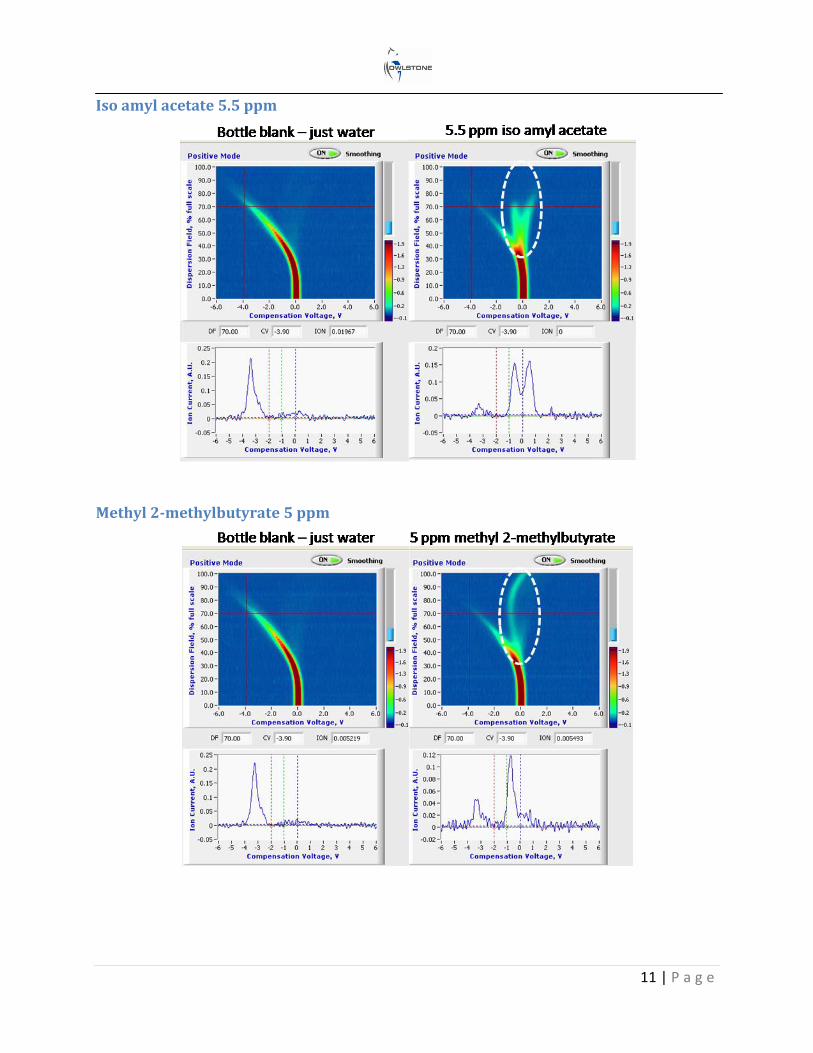
Iso amyl acetate 5.5 ppm
Methyl 2-methylbutyrate 5 ppm
12 | P a g e
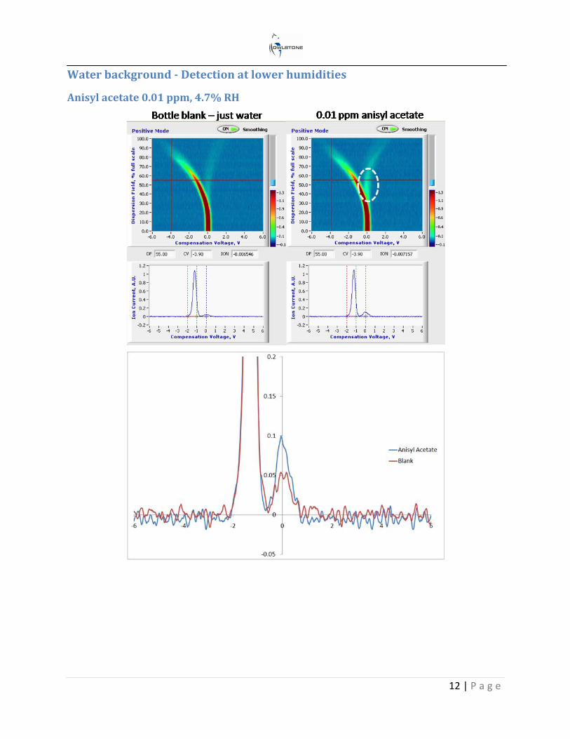
Water background - Detection at lower humidities
Anisyl acetate 0.01 ppm, 4.7% RH

13 | P a g e
Ethyl propionate 0.045ppm, 4.8% RH
Hexyl acetate 0.04 ppm, 5% RH
14 | P a g e
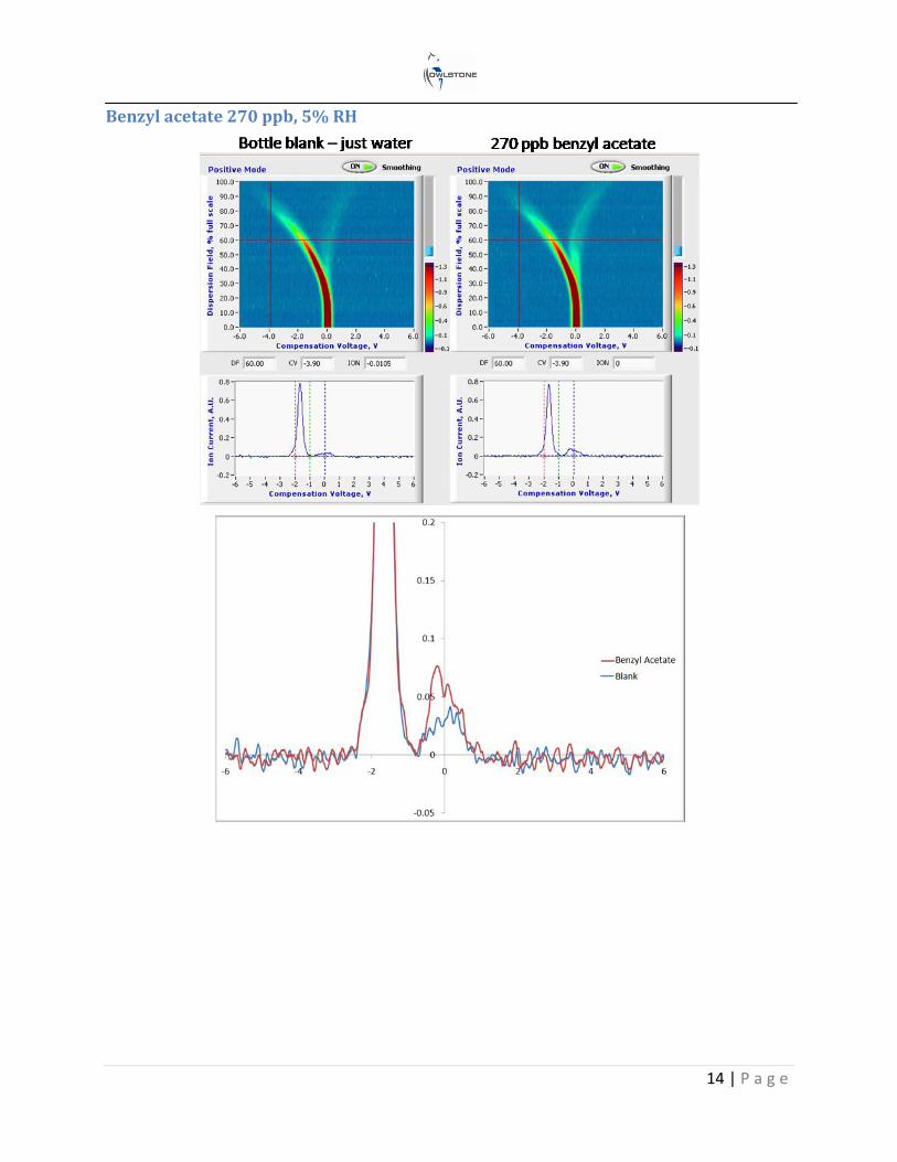
Benzyl acetate 270 ppb, 5% RH
15 | P a g e
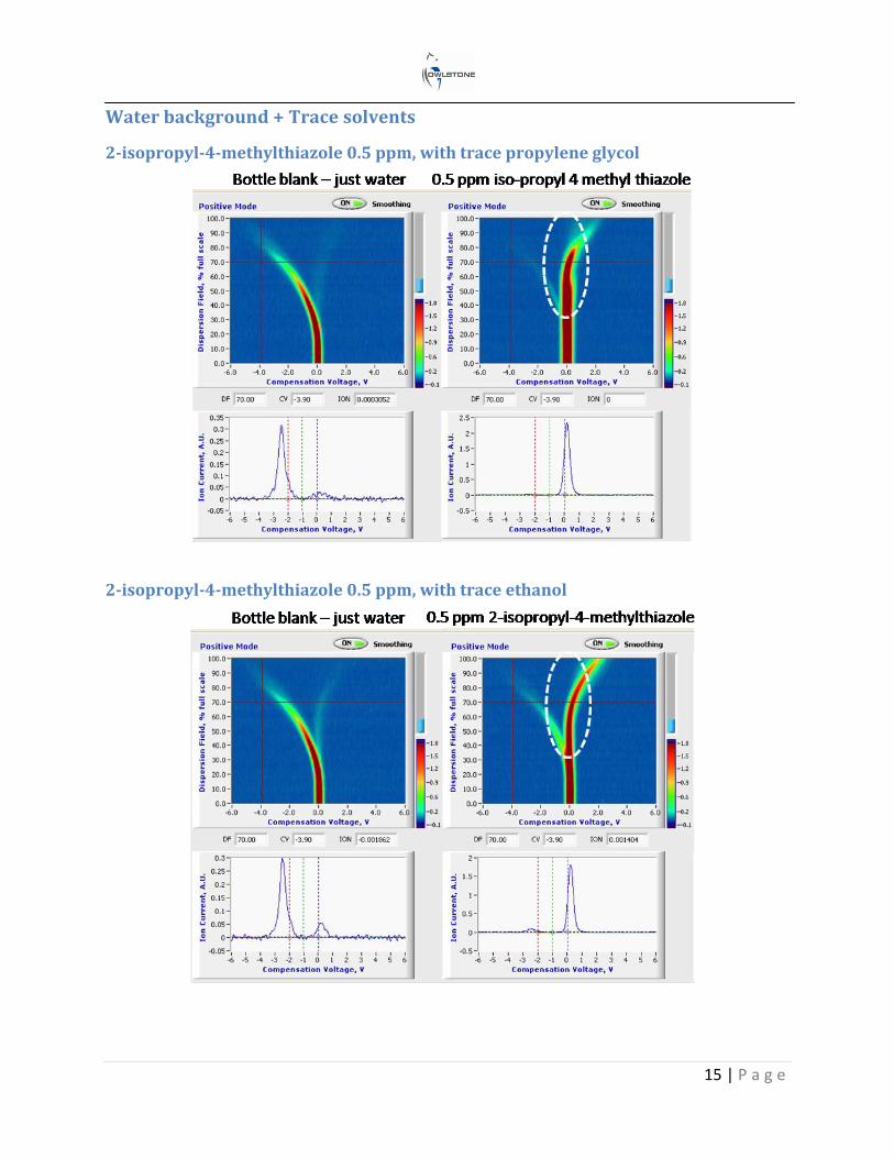
Water background + Trace solvents
2-isopropyl-4-methylthiazole 0.5 ppm, with trace propylene glycol
2-isopropyl-4-methylthiazole 0.5 ppm, with trace ethanol
16 | P a g e
Appendix A: FAIMS Technology at a Glance
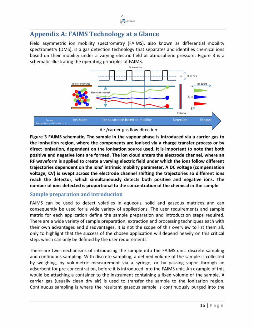
Field asymmetric ion mobility spectrometry (FAIMS), also known as differential mobility spectrometry (DMS), is a gas detection technology that separates and identifies chemical ions based on their mobility under a varying electric field at atmospheric pressure. Figure 3 is a schematic illustrating the operating principles of FAIMS.
Figure 3 FAIMS schematic. The sample in the vapour phase is introduced via a carrier gas to the ionisation region, where the components are ionised via a charge transfer process or by direct ionisation, dependent on the ionisation source used. It is important to note that both positive and negative ions are formed. The ion cloud enters the electrode channel, where an RF waveform is applied to create a varying electric field under which the ions follow different trajectories dependent on the ions’ intrinsic mobility parameter. A DC voltage (compensation voltage, CV) is swept across the electrode channel shifting the trajectories so different ions reach the detector, which simultaneously detects both positive and negative ions. The number of ions detected is proportional to the concentration of the chemical in the sample
Sample preparation and introduction
FAIMS can be used to detect volatiles in aqueous, solid and gaseous matrices and can consequently be used for a wide variety of applications. The user requirements and sample matrix for each application define the sample preparation and introduction steps required. There are a wide variety of sample preparation, extraction and processing techniques each with their own advantages and disadvantages. It is not the scope of this overview to list them all, only to highlight that the success of the chosen application will depend heavily on this critical step, which can only be defined by the user requirements.
There are two mechanisms of introducing the sample into the FAIMS unit: discrete sampling and continuous sampling. With discrete sampling, a defined volume of the sample is collected by weighing, by volumetric measurement via a syringe, or by passing vapor through an adsorbent for pre-concentration, before it is introduced into the FAIMS unit. An example of this would be attaching a container to the instrument containing a fixed volume of the sample. A carrier gas (usually clean dry air) is used to transfer the sample to the ionization region. Continuous sampling is where the resultant gaseous sample is continuously purged into the
-6+
60
Ionisation source
-
-
+
+
+ -
+ +
-
-
-
+
-
-
+
+
+ -
++
-
--
+
CV
Detector
Electrode channel
RF waveform
Air /carrier gas flow direction
Pk to Pk V 0V
Sample Ionization Ion separation based on mobility Detection ExhaustPreparation and introduction
Ion count

17 | P a g e
FAIMS unit and either is diluted by the carrier gas or acts as the carrier gas itself. For example, continuously drawing air from the top of a process vat.
The one key requirement for all the sample preparation and introduction techniques is the ability to reproducibly generate and introduce a headspace (vapour) concentration of the target analytes that exceeds the lower limits of detection of the FAIMS device.
Carrier Gas
The requirement for a flow of air through the system is twofold: Firstly to drive the ions through the electrode channel to the detector plate and secondly, to initiate the ionization process necessary for detection. As exhibited in Figure 4, the transmission factor (proportion of ions that make it to the detector) increases with increasing flow. The higher the transmission factor, the higher the sensitivity. Higher flow gives a larger full width half maximum (FWHM) of the peaks but also decreases the resolution of the FAIMS unit (see Figure 5). The air/carrier gas determines the baseline reading of the instrument. Therefore, for optimal operation it is desirable for the carrier to be free of all impurities (< 0.1 ppm methane) and the humidity to be kept constant. It can be supplied either from a pump or compressor, allowing for negative and positive pressure operating modes.
Ionisation Source
There are three main vapor phase ion sources in use for atmospheric pressure ionization; radioactive nickel-63 (Ni-63), corona discharge (CD) and ultra-violet radiation (UV). A comparison of ionization sources is presented in Table 2.
Ionisation Source Mechanism Chemical Selectivity
Ni63
(beta emitter) creates a positive / negative RIP Charge transfer Proton / electron affinity
UV (Photons) Direct ionisation First ionisation potential
Corona discharge (plasma) creates a positive / negative RIP
Charge transfer Proton / electron affinity
Table 2 FAIMS ionization source comparison
Figure 4 Flow rate vs. ion transmission factor
Figure 5 FWHM of ion species at set CV

18 | P a g e
Ni-63 undergoes beta decay, generating energetic electrons, whereas CD ionization strips electrons from the surface of a metallic structure under the influence of a strong electric field. The generated electrons from the metallic surface or Ni-63 interact with the carrier gas (air) to form stable +ve and -ve intermediate ions which give rise to reactive ion peaks (RIP) in the positive and negative FAIMS spectra (Figure 6). These RIP ions then transfer their charge to neutral molecules through collisions. For this reason, both Ni-63 and CD are referred to as indirect ionization methods.
For the positive ion formation:
N2 + e- → N2+ + e- (primary) + e- (secondary)
N2+ + 2N2 → N4
+ + N2 N4+ + H2O → 2N2 + H2O+ H2O+ + H2O → H3O+ + OH H3O+ + H2O + N2 ↔ H+(H2O)2 + N2 H+(H2O)2 + H2O + N2 ↔ H+(H2O)3 + N2
For the negative ion formation:
O2 + e- → O2-
B + H2O + O2- ↔ O2
-(H2O) + B B + H2O + O2
-(H2O) ↔ O2-(H2O)2 + B
The water based clusters (hydronium ions) in the positive mode (blue) and hydrated oxygen ions in the negative mode (red), are stable ions which form the RIPs. When an analyte (M) enters the RIP ion cloud, it can replace one or dependent on the analyte, two water molecules to form a monomer ion or dimer ion respectively, reducing the number of ions present in the RIP.
H+(H2O)3 + M + N2 ↔ MH+(H2O)2 + N2 + H2O ↔ M2H
+(H2O)1 + N2 + H2O
Dimer ion formation is dependent on the analyte’s affinity to charge and its concentration. This is illustrated in Figure 6A using dimethyl methylphsphonate (DMMP). Plot A shows that the RIP decreases with an increase in DMMP concentration as more of the charge is transferred over to the DMMP. In addition the monomer ion decreases as dimer formation becomes more favourable at the higher concentrations. This is shown more clearly in Figure 6B, which plots the peak ion current of both the monomer and dimer at different concentration levels.
Dimer Monomer

19 | P a g e
Figure 6 DMMP Monomer and dimer formation at different concentrations
The likelihood of ionization is governed by the analyte’s affinity towards protons and electrons (Table 3 and Table 4 respectively).
In complex mixtures where more than one chemical is present, competition for the available charge occurs, resulting in preferential ionisation of the compounds within the sample. Thus the chemicals with high proton or electron affinities will ionize more readily than those with a low proton or electron affinity. Therefore the concentration of water within the ionization region will have a direct effect on certain analytes whose proton / electron affinities are lower.
Chemical Family Example Proton affinity
Aromatic amines Pyridine 930 kJ/mole
Amines Methyl amine 899 kJ/mole
Phosphorous Compounds TEP 891 kJ/mole
Sulfoxides DMS 884 kJ/mole
Ketones 2- pentanone 832 kJ/mole
Esters Methly Acetate 822 kJ/mole
Alkenes 1-Hexene 805 kJ/mole
Alcohols Butanol 789 kJ/mole
Aromatics Benzene 750 kJ/mole
Water 691 kJ/mole
Alkanes Methane 544 kJ/mole
Table 3 Overview of the proton affinity of different chemical families
RIP
Monomer
Dimer

20 | P a g e
Chemical Family Electron affinity
Nitrogen Dioxide 3.91eV
Chlorine 3.61eV
Organomercurials
Pesticides
Nitro compounds
Halogenated compounds
Oxygen 0.45eV
Aliphatic alcohols
Ketones
Table 4 Relative electron affinities of several families of compounds
The UV ionization source is a direct ionization method whereby photons are emitted at energies of 9.6, 10.2, 10.6, 11.2, and 11.8 eV and can only ionize chemical species with a first ionization potential of less than the emitted energy. Important points to note are that there is no positive mode RIP present when using a UV ionization source and also that UV ionization is very selective towards certain compounds.
Mobility
Ions in air under an electric field will move at a constant velocity proportional to the electric field. The proportionality constant is referred to as mobility. As shown in Figure 7, when the ions enter the electrode channel, the applied RF voltages create oscillating regions of high (+VHF) and low (-VHF) electric fields as the ions move through the channel. The difference in the ion’s mobility at the high and low electric field regimes dictates the ion’s trajectory through the channel. This phenomenon is known as differential mobility.
Figure 7 Schematic of a FAIMS channel showing the difference in ion trajectories caused by the different mobilities they experience at high and low electric fields
Figure 8 Schematic of the ideal RF waveform, showing the duty cycle and peak to peak voltage (Pk to Pk V)
The physical parameters of a chemical ion that affect its differential mobility are its collisional cross section and its ability to form clusters within the high/low regions. The environmental factors within the electrode channel affecting the ion’s differential mobility are electric field, humidity, temperature and gas density (i.e. pressure).
-VLF
+VHF
Difference in mobility
Pk to Pk V 0V
+VHF
-VLF d
Duty Cycle = d/t t
21 | P a g e
The electric field in the high/low regions is supplied by the applied RF voltage waveform (Figure 8). The duty cycle is the proportion of time spent within each region per cycle. Increasing the peak-to-peak voltage increases/decreases the electric field experienced in the high/low field regions and therefore influences the velocity of the ion accordingly. It is this parameter that has the greatest influence on the differential mobility exhibited by the ion.
It has been shown that humidity has a direct effect on the differential mobility of certain chemicals, by increasing/decreasing the collision cross section of the ion within the respective low/high field regions. The addition and subtraction of water molecules to analyte ions is referred to as clustering and de-clustering. Increased humidity also increases the number of water molecules involved in a cluster (MH+(H2O)2) formed in the ionisation region. When this cluster experiences the high field in between the electrodes the water molecules are forced away from the cluster reducing the size (MH+) (de-clustering). As the low field regime returns so do the water molecules to the cluster, thus increasing the ion’s size (clustering) and giving the ion a larger differential mobility. Gas density and temperature can also affect the ion’s mobility by changing the number of ion-molecule collisions and changing the stability of the clusters, influencing the amount of clustering and de-clustering.
Changes in the electrode channel’s environmental parameters will change the mobility exhibited by the ions. Therefore it is advantageous to keep the gas density, temperature and humidity constant when building detection algorithms based on an ion’s mobility as these factors would need to be corrected for. However, it should be kept in mind that these parameters can also be optimized to gain greater resolution of the target analyte from the background matrix, during the method development process.
Detection and Identification
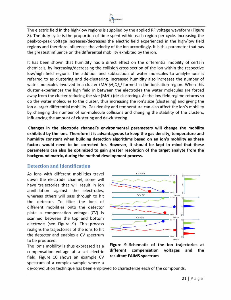
As ions with different mobilities travel down the electrode channel, some will have trajectories that will result in ion annihilation against the electrodes, whereas others will pass through to hit the detector. To filter the ions of different mobilities onto the detector plate a compensation voltage (CV) is scanned between the top and bottom electrode (see Figure 9). This process realigns the trajectories of the ions to hit the detector and enables a CV spectrum to be produced. The ion’s mobility is thus expressed as a compensation voltage at a set electric field. Figure 10 shows an example CV spectrum of a complex sample where a de-convolution technique has been employed to characterize each of the compounds.
Figure 9 Schematic of the ion trajectories at different compensation voltages and the resultant FAIMS spectrum
CV -6V
Detector
CV 6V
-6
V+6V
-0V
CV -6V
Detector
CV 6V
-6
V+6
V-
0V
CV-6V
Detector
CV 6V
-6V+6
V-0V
CV = -5V
CV = 0V
CV = 5V
22 | P a g e
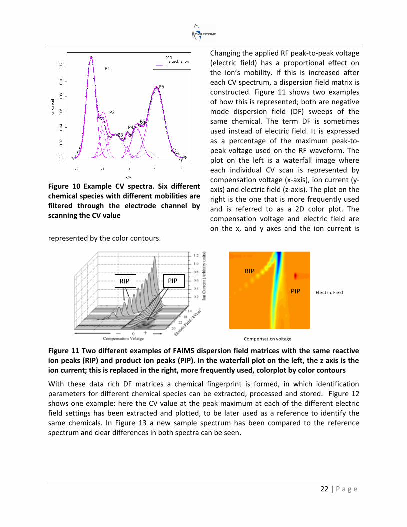
Changing the applied RF peak-to-peak voltage (electric field) has a proportional effect on the ion’s mobility. If this is increased after each CV spectrum, a dispersion field matrix is constructed. Figure 11 shows two examples of how this is represented; both are negative mode dispersion field (DF) sweeps of the same chemical. The term DF is sometimes used instead of electric field. It is expressed as a percentage of the maximum peak-to-peak voltage used on the RF waveform. The plot on the left is a waterfall image where each individual CV scan is represented by compensation voltage (x-axis), ion current (y-axis) and electric field (z-axis). The plot on the right is the one that is more frequently used and is referred to as a 2D color plot. The compensation voltage and electric field are on the x, and y axes and the ion current is
represented by the color contours.
Figure 11 Two different examples of FAIMS dispersion field matrices with the same reactive ion peaks (RIP) and product ion peaks (PIP). In the waterfall plot on the left, the z axis is the ion current; this is replaced in the right, more frequently used, colorplot by color contours
With these data rich DF matrices a chemical fingerprint is formed, in which identification parameters for different chemical species can be extracted, processed and stored. Figure 12 shows one example: here the CV value at the peak maximum at each of the different electric field settings has been extracted and plotted, to be later used as a reference to identify the same chemicals. In Figure 13 a new sample spectrum has been compared to the reference spectrum and clear differences in both spectra can be seen.
PIPRIP
Figure 10 Example CV spectra. Six different chemical species with different mobilities are filtered through the electrode channel by scanning the CV value
P1
P2
P3
P4 P5
P6
Electric Field
Compensation voltage
PIP
RIP

23 | P a g e
Figure 12 On the left are examples of positive (blue) and negative (red) mode DF matrices recorded at the same time while a sample was introduced into the FAIMS detector. The sample contained 5 chemical species, which showed as two positive product ion peaks (PPIP) and three negative product ion peaks (NPIP). On the right, the CV at the PIP’s peak maximum is plotted against % dispersion field to be stored as a spectral reference for subsequent samples.
Figure 13 Comparison of two new DF plots with the reference from Figure 10. It can be seen that in both positive and negative modes there are differences between the reference product ion peaks and the new samples
0
10
20
30
40
50
60
70
80
90
100
-0.5 0 0.5 1 1.5 2 2.5
CV / V
DF
/ % Pork at 7 Days
0
10
20
30
40
50
60
70
80
90
-1.5 -1 -0.5 0 0.5 1 1.5
CV / V
DF
/ % Pork at 7 Days
PPIP 1
PPIP 2
NPIP 1
NPIP 2
NPIP 3
PPIP 1
PPIP 2
NPIP 1
NPIP 2
NPIP 3


