Using a Vector Autoregression Framework to measure … Library Cataloguing in Publication Data A...

For further information on this or any of the

Health publications contact:

Naho Ollason

Managing Editor

LSE Health

The London School of Economics and Political Science

Houghton Street

London WC2A 2AE

Tel: + 44 (0)20 7955 3733

Fax: + 44 (0)20 7955 6090

Email: [email protected]

Website: www.lse.ac.uk/collections/LSEHealth/

Irene Papanicolas, Alistair McGuire

Using a Vector Autoregression Framework tomeasure the quality of English NHS hospitals

Working paper No: 22/2011 May 2011 LSE Health

Using a Vector Autoregression Framework to measure

the quality of English NHS hospitals


First Published in May 2011

Working paper no. 22/2011

LSE HealthThe London School of Economics and Political ScienceHoughton StreetLondon WC2A 2AE

© Irene Papanicolas, Alistair McGuire

All rights reserved. No part of this paper may be reprinted or reproduced or utilised in anyform or by any electronic, mechanical or other means, now known or hereafter invented,including photocopying and recording, or in any information storage or retrieve system,without permission in writing from the publishers.

British Library Cataloguing in Publication Data A catalogue record for this publicationis available from the British Library ISBN [978-0-85328-464-2]

Corresponding authorIrene Papanicolas and McGuire (2011)London School of Economics and Political ScienceHoughton StreetLondon WC2A 2AEEmail: [email protected]

1

2

Abstract

In order to address the problem of poor quality information available to health care providerstoday, McClellan and Staiger (1999) developed a new method to measure quality, which addressessome key limitations of other approaches. Their method produces quality estimates that reflectdifferent dimensions of quality and are able to eliminate systematic bias and noise inherent in thesetypes of measures. While these measures are promising indicators, they have not been applied toother conditions or health systems since their publication. This paper attempts to replicated their1999 method by calculating these quality measures for English Hospitals using Hospital EpisodeStatistics for the years 1996-2008 for Acute Myocardial Infarction (AMI) and Hip Replacement.Using the latent outcome measures calculated previously, Vector Autoregressions (VARs) are usedto combine the information from different time periods and across measures within each condition.These measures are then used to compare current and past quality of care within and across NHSAcute Trusts. Our results support that this method is well suited to measure and predict providerquality of care in the English setting using the individual patient level data collected.

Keywords: Measuring Quality; Vector Autoregressions; Health.

Contents 3

Contents

1 Introduction 4

2 Background 11

3 Methodology 14

4 Data 17

5 Results 19

5.1 AMI . . . . . . . . . . . . . . . . . . . . . . . . . . . . . . . . . . . . . . . . 22

5.2 Hip Replacement . . . . . . . . . . . . . . . . . . . . . . . . . . . . . . . . . 29

5.3 Comparison of Indicators . . . . . . . . . . . . . . . . . . . . . . . . . . . . 35

6 Discussion 39

A Appendix: Comparison of Indicators 47

4 1 Introduction

1 Introduction

The desire to measure the quality of hospital care dates back to the advent of medicineitself. Yet, the measurement of hospital quality is no easy feat. Health care is complex,multidimensional and the link between clinical practice and patient outcomes is oftentenuous at best. Many hurdles face those who attempt to measure quality starting withthe seemingly simple task of defining it. As far back as ancient Greece, the challenge indefining quality of care resulted in using list of attributes, categories or features to aidin its conceptualizations. The ancient civilizations of Egypt and Babylon recognized thatpoor quality care can lead to harm, and good quality care to the absence of harm, howeverstill struggled with a better way to measure it than simply focusing on the final outcomeof care (Reerink, 1990). Indeed, up until the pioneering work of Nightingale, Codman andDonabedian, the notion of quality of care while very real in terms of being recognized andappreciated, was a mystery in terms of how to palatably define or measure it.

The first proponents of routine clinical outcome measurement were Florence Nightingale(circa 1860) and Ernest Codman (circa 1900). Nightingale pioneered the systematic andrigorous collection of hospital outcomes data in order to understand and improve perfor-mance. While Codman advocated the “end results idea”, essentially the common sensenotion of following every patient treated for long enough to determine whether their treat-ment was successful, and if not to understand and learn from the failures which occurred.Unfortunately, political and practical barriers prevented both these ideas from becomingfully adopted until the last twenty years. Currently, quality of hospital care is often con-ceptualized with regards to the performance in different domains, and in its measurementindicators range beyond clinical outcomes, such as clinical process measures and resourceutilization measures. Avedis Donabedian, whose name is synonymous with quality mea-surement, advocated the measurement of structure process and outcome rather than theuse of only outcomes to measure quality. He argued that “good structure increases thelikelihood of good process, and good process increases the likelihood of good outcome”(Donabedian, 1988). Indeed many of the indicators used for quality measurement areoften thought of in terms of this framework, and increasingly quality management policiesuse combinations of the three types of indicators.

Although clinical outcome measures are the gold standard for measuring effectiveness inhealth care, their use can be problematic, for example if the outcomes cannot realisticallybe assessed in a timely or feasible fashion, or when trying to understand the contributionof health services to health outcomes. Thus many health services performance initiatives

5

use measures of health care process instead of, or in addition to, measures of outcome.Process measures have certain distinct advantages, for example, they are quicker to mea-sure, and easier to attribute directly to health service efforts (Brook et al., 1996). Inaddition they are commonly considered a better measure of quality as they examine com-pliance with what is perceived as best practice. However, they may have less value forpatients unless they are related to outcomes, and may be too specific focusing on particularinterventions or conditions. Moreover, process measures may ultimately ignore the effec-tiveness or appropriateness of the intervention and pre-judge the nature of the responseto a health problem, which may not be identical in all settings, such as for patients whohave multiple morbidities (Klazinga, 2011). In recent years another important develop-ment in the assessment of health service performance has been the growing use of patientreported outcome measures. These type of measures typically ask patients to assess theircurrent health status, or aspects of health problems (Fitzpatrick, 2009). In England, theroutine use of Patient Reported Outcome Measures (PROMS) is growing, with wide-scaleadoption in the NHS from 2009 for certain elective procedures.

However, amongst these different measures and dimensions, clinical outcome measuresarguably carry the most weight as they are often the most meaningful for stakeholdersand more clearly represent the goals of the health system. Even Donabedian himself con-cluded that, “outcomes, by and large, remain the ultimate validation of the effectivenessand quality of medical care” (Donabedian, 1966). In the past decades, many industrial-ized countries have invested large amounts in the development and routine collection ofhospital outcome indicators. Indicators are being developed, tested and used in countriessuch as Austria, Finland Spain, Italy, France, Germany, Australia, the UK and the US,where administrative databases and medical records are able to provide large-scale sourcesof individual patient level data. These databases allow researchers to easily and relativelycheaply calculate hospital-specific mortality rates which often serve as outcome-based mea-sures of quality. It is easy to see why this type of measure is desirable. A simple indicatorthat allows the identification of ‘good’ and ‘bad’ hospitals can serve as instruments todirect policy and or to inform patient decisions. Indeed for some conditions, routinelyavailable data or this sort has been shown to be as good a predictor of death as someexpensive clinical databases (Aylin et al., 2007).

As measures of health outcome are increasingly used to inform policy, statistical re-searchers have made efforts to address some of the methodological issues associated withthem. For example, it is well known that a patient’s outcome will be influenced by theseverity of their condition, their socio-economic status as well as the resources allocatedto their treatment. In such cases, it is critical to employ methods of risk adjustment

6 1 Introduction

when using and comparing indicators to help account for these variations in patient pop-ulations. Failure to risk adjust outcome measures before comparing patient performancemay result in misinterpretation of data which can have serious implications for qualityimprovement and policy (Lisa I Iezzoni, Lisa I Iezzoni). Typically, some sort of risk ad-justment technique is employed to address these attribution problems, and control for theother influencing factors. However, many different risk-adjustment mechanisms exist, andare applied differently by different users (Iezzoni, 1994). Thus risk-adjusted measures maynot always be comparable with one another (Iezzoni et al., 1996).

Hospital standardized mortality ratios (HSMR) are common risk-adjusted measures usedto evaluate overall hospital mortalities. Initially developed by Jarman (Jarman et al.,1999), HSMRs compare the observed numbers of deaths in a given hospital with theexpected number of deaths based on national data, after adjustment for factors that affectthe risk for in-hospital death, such as age, diagnosis and route of admission (Shojaniaand Forster, 2008). However, despite their prolific use, many authors express concernsas to the degree of true quality information these indicators hold and implore users ofthis information to exercise caution in drawing conclusions from them (Birkmeyer et al.,2006; Dimick et al., 2004; Lingsma et al., 2010; Mohammed et al., 2009; Normand, Wolf,Ayanian, and McNeil, Normand et al.; Powell et al., 2003; Shahian et al., 2010). In part,these concerns represent skepticism about how good risk adjustment techniques are atcontrolling for differences in for case mix or chance variation. But also, mortality may notalways be a valid indicator of quality (Lisa I Iezzoni, Lisa I Iezzoni; Shojania and Forster,2008). For, even when outcome measures are risk adjusted they still run the risk of notaccounting for factors that cannot be identified and measured accurately.

Indeed, measures of risk may not be uniformly related to patient outcomes across allhospitals. Certain systematic factors which bias results when these differences are nottaken into account. Mistaking such errors for differences in quality is known as “case-mix fallacy”. Systematic errors of these sort will lead to erroneous conclusions concerninga variables true value. For example, patterns of use of emergency services may indicatehigher degrees of illness in some areas, but poor availability of alternative services in others(Wright and Shojania, 2009). It would me misleading to adjust the data across hospitalsaccording to only one of these assumptions. Mohammed et al. (2009) find systematicassociations between hospital mortality rates and the factors used to adjust for case-mix inEnglish Dr. Foster data. Thus, using these measures for case-mix adjustment may actuallyincrease the bias that they are intended to reduce (Lilford et al., 2007; Powell et al., 2003).In these cases standardized mortality ratios, or other risk-adjustment methods may also bemisleading. In order to avoid these types of errors it is critical that data collection methods

7

are carefully designed and implemented (Terris and Aron, 2009). Most recently Shahianet al. (2010) present evidence suggesting that the methodology used to calculate hospitalwide mortality rates is instrumental in determining the relative ‘quality’ assigned to aparticular hospital. The authors note that rather than suggesting a particular preferredtechnique for the calculation of hospital mortality, they call into question the very conceptof the measurement of hospital-wide mortality.

Moulton (1990) notes that using aggregate variables, such as average death rates, in com-bination with individual observations by trust or site to determine relationships throughregressions or other statistical models runs the risk of producing downwards biased stan-dard errors, and possibly exaggerating the significance of certain effects based on spuri-ous associations. Moreover, while some deaths are preventable, or more dependent ontreatment, it is not sensible to look for differences in preventable deaths by comparingall outcomes from one provider. Focusing on mortality rates associated with procedureswhere the quality of care is known to have a large impact on patient outcomes, such asthose that are heavily dependent on technical skill, is in fact more informative (Lilfordand Pronovost, 2010).

Indeed, focusing on certain conditions could be considered an extreme form of risk adjust-ment, where measures focus only on particular conditions, rather than creating organiza-tion wide outcome measures. Surgical mortality rates for specific conditions or procedureshave become more popular as they are able to identify key areas where health system qual-ity is more likely to influence outcomes, and where medical progress has been instrumentalin improving outcomes. Popular outcome indicators of this sort are 30-day mortality ratesfor acute myocardial infarction (AMI) and Stroke. Better treatment of AMI in the acutephase has led to reductions in mortality (Capewell et al., 1999; McGovern et al., 2001).The last few decades have seen a dramatic change in care for AMI patients Klazinga (2011)first with the introduction of coronary care units in the 1960s (Khush et al., 2005) andthen with the advent of treatment aimed at restoring coronary blood flow in the 1980s (Gilet al., 1999). Aside from the contributions from medical technology, improved processeshave also contributed to the improvement in outcomes. Research showed that the timefrom AMI occurrence to re-opening the artery is a key driver of prognosis, and since careprocesses were changed radically. It is now common for emergency medical personnel toadminister drugs, such as aspirin, during patients transport to hospital and emergencydepartments have instituted procedures to ensure that patients receive definite treatmentwith thrombolysis or catheterisation within minutes of arrival (Klazinga, 2011). Moreoverthe proven link between identified care processes and patient outcomes, for conditions suchas AMI, allow researchers to be more confident in making judgements about quality and

8 1 Introduction

the end result of care. Indeed, there has been considerable work that has used AMI asa proxy for quality both in England (Bloom et al., 2010; Propper et al., 2004, 2008) andinternationally (Kessler and McClellan, 1996, 2011; McClellan and Staiger, 1999; Shen,2003).

The Organization for Economic Co-operation and Development (OECD) Health CareQuality Indicators (HCQI) project, initiated in 2002, which aims to measure and comparethe quality of health service provision in the different countries identifies key quality vari-ables that can be used at the acute care level1. These indicators include case-fatality ratesfor AMI and Stroke (OECD, 2010). The Agency for Healthcare Research and Quality inthe US, identified seven operations for which they recommended surgical mortality as aquality indicator: Coronary Artery Bypass Graft (CABG) surgery, Repair of AbdominalAortic Aneurysm, Pancreatic Resection, Esophageal Resection, Pediatric Heart Surgery,Craniotomy and Hip Replacement (Dimick et al., 2004). However, even in cases wherethere is an established link between treatment and quality, it is not necessarily the casethat surgeries are performed frequently enough, in all hospitals, to reliably identify hos-pitals with increased mortality rates. Indeed, Dimick et al. (2004), attempted to identifyhow many hospitals had an appropriate sample size to determine quality based on theseseven conditions. They found that apart from CABG surgery, the remainder of operationsfor which surgical mortality was advocated as a suitable indicator were not performedfrequently enough to make valid assessments of quality. Indeed further work on the re-lationship between hospital volumes and outcome indicate that mortality rates are poormeasures of quality when small numbers of procedures are performed, unfortunately mostprocedures are not performed frequently enough to allow valid assessment of procedure-specific mortality at the individual hospital level (Birkmeyer et al., 2002). Indeed, mostobserved variation across hospitals and across time is actually, as a consequence, fromrandom variation (good or bad luck) and does not reflect meaningful changes in quality(Dimick and Welch, 2008).

Another common outcome measure at the hospital level are readmission rates. The mea-sure has become increasingly popular despite the fact that it cannot always be attributedto the quality of care delivered by the hospital. Indeed, McClellan and Staiger (1999) notethat high readmissions may be easily misinterpreted as indicators of poor quality whenin some cases they may indicate good quality treatment of severe patients. Moreover,

1 As the HCQI project is concerned with overall health system quality it also identifies suitable qual-ity indicators in other health system domains, including patient safety, health promotion, protectionand primary care, patient experiences, cancer care and mental health care. For more information seehttp://www.oecd.org/health/hcqi.

9

readmissions may be the result of poor quality care of other parts of the health system(primary care), behavioural factors (poor adherence), or even the result of good qualitycare; as hospital technology improves patients may survive, but with worsened morbidityand subsequent episodes of hospital readmission. Benbassat and Taragin (2000) concludethat readmission indicators are not good measures of quality of care for most conditions,as there is large variation in the percentage of the indicator that can be attributed poorquality care. Their own study using reports of different readmission indicators for variousconditions indicated a range between 9% – 50%. They note that readmissions for specificconditions, such as Child Birth, Coronary Artery Bypass Grafting and Acute CoronaryDisease as well as approaches that ensure closer adherence to evidence based guidelines,may be more appropriate.

However, after initial use in the US, there are now a growing number of European countriesthat measure readmission rates more systematically as a health service outcome (Klazinga,2011). A recent literature review conducted by Fischer et al, (2010), indicated that ofthe 360 studies reviewed which used readmission rates as an outcome indicator, only 23focused on the validity of the indicator and only 14 looked at the specific source of dataused to calculate the indicators. The authors concluded that routinely collected data onreadmissions alone is most likely insufficient to draw conclusions about quality. Some ofthe major problems linked to this conclusion was evidence of inaccurate and incompletecoding of the indicator, and little evidence to indicate that readmissions are related withquality of care carried out.

While investigating mortality and readmission rates by different condition may allow aclearer relationship between outcome and quality of care, other challenges such as randomerror data quality still persist. Powell et al. (2003) note that variations in outcome will beinfluenced by change variability which can manifest itself in Type 1 or Type 2 errors as wellas data quality. Both these issues are important, and while the former can be accountedfor to some degree using statistical tools the later can seriously undermine conclusionsmade using the data. The best way to reduce the likelihood of both these types of errorsis to have more data, or more precision in the way they are collected. As routine datacollection mechanisms are still being developed and improved there is no way to completelyavoid this issue. Yet, as Spiegelhalter et al. (2002) note it would be advantageous to havebetter data on morbidity collected, as mortality data is in most circumstances sufficientlyrare, and thus of limited value in monitoring. Regardless, known limitations in the datashould always be made explicit when it is used.

Over the past two decades, much empirical research has been done to create improved

10 1 Introduction

adjustment mechanisms to make the best use of this information (Iezzoni, 2003). As moreorganizations begin to use performance systems to make judgements about health servicequality and support decision making, more work has been concerned with methodologicaltechniques that can be used to create suitable profiles of provider quality (Landrum et al.,2000). Different statistical techniques have been used to this end, investigating one di-mension of care, including Bayesian hierarchical regression models (Normand et al., 1997;Christiansen and Morris, 1997) and maximum likelihood estimates (Silber et al., 1995).These models control for differences in cases per hospital, thus reducing the noise whichmay produce large differences between observed and expected mortality between hospitalswith different sample sizes – due primarily to sampling variability.

However, as quality is multidimensional, this type of focus will limit the focus of compar-ison across providers, and result in misleading results. However, reporting on too manydifferent types of indicators may create confusion or overwhelm users of performance in-formation, when there are contradictory indicators or simply too much information. Socalled composite measures, or aggregated measures, may address some of these problems.However there is often much controversy surround them because of the methods requiredto construct them which often involve weighing different aspects of performance. Yet,different methodological studies have been undertaken to try to find suitable methods toaddress these issues (Landrum et al., 2000).

Latent variable models have been used to account for the correlation among performancemeasures and to measure the quality of providers. This type of methodology assumes anunobservable (latent) trait, such as quality, contributes to the attainment of an ultimateoutcome. Correlation among different measures is induced by variability in the latenttrait of any one provider, which represents the summary of the unobserved quality theyare able to deliver (Landrum et al., 2000). Originally these types of models were used inpsychology research (Bentler, 1980; Cohen et al., 1990), but have been applied to manydisciplines, including economics where they have been used to measure areas that are notdirectly observable, such as quality of life (Theunissen et al., 1998). One of the advantagesto using this methodology is that it can deal with multidimensionality of data, as it is ableto aggregate a large number of observable variables to represent an underlying concept.Previous work (Papanicolas and McGuire, 2011) has used this approach to measure thequality of different English NHS hospitals in providing services over the period 1996-2008for seven different conditions. However, the variability present in latent measures, or inour case in latent quality across providers, will include both a systematic component anda random component. The former can be explained by provider specific covariates and thelatter by chance. While the systematic components will also include measures of quality,

11

they may also include other systematic differences that contribute to outcome, such asdeprivation or severity, which may bias the measures (Mohammed et al., 2009). Such bias isreferred to as systematic error, as discussed previously. In order to correct for these biases,as well as some of the noise still present in the estimates, and create better measures ofquality McClellan and Staiger (1999) proposed using multivariate autoregression methods.

We use this method to evaluate quality for English hospitals using English patient leveldata. Their method uses vector autoregressions (VARs) to capture dynamic interactionsin the time series and across measures. This step allows information from the dynamicinteractions of outcomes over time and across dimensions to be used to filter out more of thenoise captured by the measures, and also use the time series and cross sectional informationcontained in the estimates to further adjust them. Moreover, the VAR methodology iscommonly used for forecasting, and thus can be used to predict and forecast hospitalquality extremely well. This chapter reviews the entire methodology and uses it to replicatethe McClellan and Staiger (1999) quality measures for English hospitals. These modelsare able to create smoothed out hospital rates of mortality and complications over timeas well as to forecast future performance. This paper applies the McClellan and Staiger(1999)technique to our previously estimated latent estimates calculated in Papanicolasand McGuire (2011) and assesses the performance of the two measures in order considerthe advantages and disadvantages of the different methodologies.

2 Background

In health economics, and many other areas of applied economics, we face problems ofendogeneity amongst dependent and independent variables. Endogeneity can occur incases where there is a two-way influence between the independent and dependent variables.This influence can arise from autoregression with autocorrelated errors, omitted variablebias, simultaneity between variables as well as measurement and/or sample selection error.Different methodological techniques have been adopted to deal with this issue, such asinstrumental variable (IV) methods, simultaneous equation models, non-linear techniquesand GMM estimators, such as those outlined in Wooldridge (2002). Yet this problemof endogeneity is not unfamiliar to economists who have come across the same problemswhen attempting to explain the relationships among money, interest rates, prices andoutput. In 1980, Christopher Sims (1980) championed the VAR approach which tookaway many of the restrictions models impose and allowed the data to be modelled in anunrestricted reduced form, where all variables are treated as endogenous. Predictions of

12 2 Background

the VAR model performed well, and so the technique has become popular in economicsdespite critiques that it is atheorectical. The basic idea behind the model is to treat allvariables symmetrically, such that variables which that we are not confident are exogenousare modelled as endogenous. This leads to an n-equation, n-variable linear model, whereeach variable is explained by its own lagged values, plus the current and past values of theother lagged variables. While VAR models are often used in macroeconomics to analysethe relationship between different policy tools, they have rarely been used in the area ofhealth economics.

This chapter considers using a VAR methodology similar to the McClellan and Staiger(1999) method used to create better quality indicators that will control for these issues butalso use them to inform their estimation. The simplest form of a VAR is a first-order VARspecification, VAR(1), where the longest lag length modelled is unity. Different specifica-tions of the model however are also able to incorporate more lags. Indeed identifying thecorrect number of lags is important in order to specify the model correctly, and is likelyto influence the results. There are various tests available that indicate how many lags areappropriate, including the Akaike information criterion (AIC) and the Schwartz criterion.

Stock and Watson (2001) also note that the VAR can come in three different varieties, eachof which places different restrictions upon the data being modelled, these are: reducedform, recursive and structural. A structural VAR use theory to produce instrumentalvariables that can test contemporaneous links between variables (Stock and Watson, 2001).In practice structural VARs differ considerably from their reduced form and recursivecounterparts, because of the restrictions placed upon the model. As we do not use thistype of VAR we will not go over it in detail2. A reduced form VAR expresses each variableas a linear function of its own past values, the past values of all other variables beingconsidered and a serially uncorrelated error term. In our evaluation of quality a VAR(1)model of this type would be represented by this simple system:

D30ht = α + β1D30h(t−1) + β2D365h(t−1) + β3R28h(t−1) + β4R365h(t−1) + D30ht

D365ht = α + β1D365h(t−1) + β2D30h(t−1) + βR28h(t−1) + βR365h(t−1) + D365ht

R28ht = α + β1R365h(t−1) + β2D30h(t−1) + β3D365h(t−1) + β4R28h(t−1) + R28ht

R365ht = α + β1R365h(t−1) + β2D30h(t−1) + β3D365h(t−1) + β4R28h(t−1) + R365ht . (1)2 For an in-depth discussion on structural VARs see Stock and Watson (2001); Enders (2004).

13

Each equation in this system defines an outcome of interest and is estimated by OrdinaryLeast Squares (OLS). The outcomes are 30-day mortality, D30ht, from the disease underconsideration, one-year mortality, D365ht, as well as 28-day readmissions R28ht and one-year readmissions, R365ht . The subscript t denotes time in terms of years, and t − 1occruances in the past yer. The error terms represent the ‘surprise’ movements in thevariables after the past variables have been taken into account. If the different variablesare correlated with each other, than the error terms in the reduced form model will alsobe correlated across equations.

A recursive VAR constructs the error terms in each regression to be uncorrelated with oneanother by including some contemporaneous values of the variables in the regression. Soour system from above, would be modified to look something like:

D30ht = α + γ1D365ht + γ2R28ht + γ3R365ht + β2D365h(t−1)

+ β3R28h(t−1) + β4R365h(t−1) + D30ht

D365ht = α + γ1D30ht + γ2R28ht + γ3R365ht + β1D30h(t−1) + β2D365h(t−1)

+ β3R28h(t−1) + β4R365h(t−1) + D365h

R28ht = α +γ1D30ht +γ2D365ht +γ3R365ht +γ3R365ht +β1D30h(t−1) +β2D365h(t−1)+

β3R28h(t−1) + β4R365h(t−1) + R28ht

R365ht = α + γ1D30ht + γ2D365ht + γ3R28ht + β1D30h(t−1) + β2D365h(t−1)

+ β3R28h(t−1) + β4R365h(t−1) + R365ht . (2)

Equations (2) are not reduced form equations, for example D30ht will have a contempo-raneous effect on the other three quality variables, and they will have a contemporaneouseffect on D30ht. This system can be better represented in matrix algebra, allowing theVAR model to be represented in standard form (Enders, 2004). Again each regressioncan be estimated by OLS, however if the right hand variables are not identical, becausesome contemporaneous effects are dropped than estimation by OLS will no longer provideuncorrelated error terms. In this case a Seemingly Unrelated Regression (SUR) may proveto be more efficient.

As VARs involve current and lagged values of multivariate time series they are able to

14 3 Methodology

capture co-movements between variables that other models cannot. Thus, VAR models canbe very useful for data description. The McClellan and Staiger (1999) methodology usesa reduced form VAR between the latent quality variables to understand the interactionsbetween the variables which are thought to be co-determined. Indeed by closely studyingthe residuals and the coefficients they are able to better understand just how persistentquality is for various conditions. The relationship amongst different quality indicators andinformation about the variables which is important in their interpretation. Following thisanalysis, the authors use the output produced from the VAR model to create smoothedtime-series estimates of each of the outcome variables that take into account the time-series and cross-sectional variations they have identified. The empirical steps to thisprocess taken to replicated this process are reviewed in detail the following section beforethe results are presented and discussed.

3 Methodology

Hospital performance over the period 1996 to 2008 is evaluated by a two step process, asoutlined by McClellan and Staiger (1999). The first step, undertaken in Papanicolas andMcGuire (2011), derives latent outcome measures at the hospital level (h) by estimatingpatient level (i) regressions replicated below. The patient level regressions include hospitalfixed effects (β) and a set of patient characteristics,

φX, known to influence outcomes

(age, gender, deprivation, co-morbidities, and elective or emergency treatment). The re-gressions are run separately for each year (t) and outcome measure (k), and the hospitalintercepts, representing the mean value of outcomes of each hospital holding patient char-acteristics constant across all hospitals, are extracted and used to create a new dataset atthe hospital level.

Y kiht = βqk

1h +

φXjht + uiht . (3)

As explained in detail in Papanicolas and McGuire (2011), the latent measures, β, describethe rate of change in outcomes as explained by risk-adjusted hospital quality. This chapteruses these latent measures in a VAR framework to create new quality measures whichdescribe, summarize and forecast hospital quality. The newly constructed dataset containsQh a 1 × TK vector of the estimated latent hospital outcome for hospital h, adjusted for

15

differences in patient characteristics, such that:

Qh = qh + h ,

where qh is a 1 × TK vector of the true hospital effects for hospital h, and h is theestimation error (which is mean zero and uncorrelated with qh). The variance of h isestimated from the patient level regressions (equation (3)) and is equal to the variance ofthe regression estimates Qh, where Ωjh represents the covariance matrix of the hospitaleffects estimates for hospital h in year t. Or simply:

E(htht) = Ωht

E(htht) = 0, for t = s .

Thus, the estimation problem McClellan and Staiger (1999) lay out is how to provideestimates of Qh to predict qh. They propose creating a linear combination of each hospital’sobserved measures in such a way that minimizes the mean squared error of the predictions,conceptualised as running the following hypothetical regression:

qkht = Qhtβ

kht + ωiht (4)

They note that equation (4) cannot be estimated directly, as q represents unobservedperformance and the optimal β varies by hospital and year. Thus, the measurementchallenge is to predict the true hospital effect, q, from its noisy estimate Q. The idea isto attenuate the coefficient of Q towards zero, such that a prediction of q can be derivedthat will reduce the noise without distorting the true effect. This is a similar idea to asmoothing techniques as outlined, for example, in Titterington et al. (1985).

While equation (4) can not be directly estimated, the parameters of the hypotheticalregression can be estimated from the existing data. The minimum least squared predictoris given by:

W (qh|Qh) = Qhβ ,

where

β = [E(QhQh)]−1E(Q

hqh) . (5)

16 3 Methodology

This best linear predictor can be calculated using the following estimates:

E(QhQh) = E(q

hqh) + E(hh) (6)

E(QhQh) = E(q

hqh) , (7)

where E(hh) is estimated using the individual patient level estimates of the covariance

matrix for the parameter estimates Qh, which we call Sh. Sh varies among hospitals.E(q

hqh) can be estimated by E(QhQh − Sh) = E(Q

hqh). Plugging these estimates intoequation (5) allows the calculation of the desired least squares estimates, such that:

qht = Q[E(QhQh)]−1E(Q

hqh) = Qh[E(qhqh) + E(

hh)]−1E(qhqh) . (8)

Using estimates (6)and (7), the R-squared statistic can also be calculated, based on theleast squared formula.

Estimation of equation (8) provides the basis for the second step of the methodology,undertaken in this chapter. McClellan and Staiger (1999) coin these estimates ‘filteredestimates’ as they optimally filter out the estimation error of the observed quality mea-sures. They note three attractive properties of the filtered estimates. First, that allowsinformation for many years and different indicators to be combined in a systematic man-ner. Second, by nature of their construction, these estimates are optimal linear predictorsfor mean squared error. Finally, the estimates are simple to construct using standardstatistical software.

Given the time-series nature of the data, information of the performance in each hospitaleffect over time is used to better predict and further forecast the outcome measures. Usinga VAR model, further structure is imposed on the filtered estimates, by assuming thateach performance measure in a given its past performance, plus a contemporaneous shockthat can be correlated across the different outcome measures. Thus a first order VARmodel for qht(1 × K) is estimated, where:

qht = qh,t−1Φ + vht . (9)

Z = V (vht) the (K × K) variance matrix of the residuals, and Γ = V (qh(t=1)) the (K ×K) initial variance matrix from the first year of the data sample are also estimated. Φrepresents a (K × K) matrix containing the estimates of the lag coefficients. The VAR

17

structure implies:

E(QhQh) − Sh = E(q

hqh) = f(Φ, Z, Γ) . (10)

Using the parameters estimated from the VAR model we are able to estimate equation(10), using the Broyden algorithm in eViews to estimate non-stochastic predictions, or the‘filtered outcome measures’.

The above analysis is estimated using a large pooled cross section that spans over manyindividuals and providers. The first part of the analysis, reviewed in detail in Papanicolasand McGuire (2011), is performed using the statistical package STATA, the remainderof the analysis is undertaken in eViews, which includes more options to perform time-series analyses, and especially the VAR model. The size and amount of information oneach patient and provider allows us to avoid many of the technical and methodologicalchallenges presented in time series analysis.

4 Data

Similar to Papanicolas and McGuire (2011), the data used in this paper is Hospital EpisodeStatistics (HES) accessed through Dr. Foster. Hospital episode statistics (HES) containrecords for all NHS patients admitted to English hospitals in each financial year (April 1to March 31), with information on all medical and surgical specialties, including privatepatients treated in NHS hospital trusts. Diagnosis of patients are coded using ICD-10 (in-ternational statistical classification of diseases, tenth revision) codes while procedures usethe UK Office of Population Censuses and Surveys classification (OPCS4). The data avail-able in the HES database contains patient characteristic data (e.g. gender, age), clinicalinformation (e.g. diagnoses, procedures undergone), mode of admission (emergency, elec-tive), outcome data (mortality, readmission, discharge location) as well as details on theamount of time spent in contact with the health system (waiting times, date of admission,date of discharge) and details of which hospital the patient was treated in.

Data on gender and age are used as explanatory variables in the analysis, as is a variableindicating whether the treatment undergone was an elective procedure. The Charlson co-morbidity index which predicts the 1 year mortality for a patient who may have a range ofco-morbid conditions was used to control for severity of patients. This index is constructedby assigning a score to each condition depending on the risk of dying associated with it,and summing these scores up (Charlson et al., 1987). Finally, socio-economic status was

18 4 Data

measured using the Carstairs index of deprivation. This index is based on four censusindicators: low social class, lack of car ownership, overcrowding and male unemployment,which are combined to create a composite score. The deprivation score is divided intoseven separate categories which range from very low to very high deprivation.

This paper analyses data provided for the financial years 1996-2008, for the conditions ofAcute myocardial infarction (AMI) and Hip Replacement. The data for these conditionswas extracted based on the ICD-10 and OPCS 4.3 classification codes indicated in Table1. Due to problems with the sample sizes for some of the years before 2000 for AMI theseyears were not included in the analysis. Moreover, any hospital trust that had less than10 admissions throughout the entire period of analysis was dropped from the analysis.Moreover, any primary care trusts, private trusts acting as NHS providers and social caretrusts were also excluded. For the sample of patients admitted with AMI, only emergencyadmissions were examined, and only for patients with a length of stay greater than twodays.

This paper builds on the methods used in Papanicolas and McGuire (2011) which usedindividual patient mortality rates and readmission rates at different intervals to contractlatent outcome measures at the hospital level, as outlined in the methodology sectionabove. These latent measures are collected into a new data set at the hospital level,distinguished by hospital identifiers and variables indicating the year of the measure. Inorder to conduct the analysis described above all hospitals with missing years of dataare dropped from the sample. The sample size described in terms of number of hospitalsand average number of cases per hospital across all years are presented in Table 1. Datawere collected on seven conditions to assess the generalisability of the method. The sevenconditions are Acute Myocardial Infarction (AMI), Myocardial Infarction (MI), IschemicHeart Disease (IHD), Congestive Cardiac Failure (CCF), Stroke, Transient Ischemic At-tack (TIA) and Hip Replacement. However, we reprot on two conditions in detail, AMIand Hip Replacement, for the sake of brevity and as the general conclusion hold for allthe conditions. More detail can be obtained by contacting the authors.

Tab. 1: Summary statistics of the sample of hospitals included.

Condition ICD-10/ OPCS 4.3 codes YearsAnalysed

Number ofHospitals

Average Cases perHospital per year

AMI ICD-10: I21 2000-2008 119 331Hip OPCS4.3: W37-W39

W46-W48 W581996-2008 120 332

19

5 Results

The methodology of this chapter uses VAR models to describe and summarise hospitalquality. By quantifying what is known about the different dimensions of measured qualityand the time trend associated with the different latent outcome measures. The results ofthis chapter attempt to illustrate how well the filtered estimates perform at predicting insample hospital quality and forecasting out of sample hospital quality. This is done bycomparing the filtered measures to the latent measures diagrammatically as to visualizehow the methodology reduces the noise in the estimates, by measuring the signal to noiseratio of the filtered estimates, and by estimating the goodness of fit measures of theestimates. Each of these steps is explained in more detail below. This section shows thatin all of these areas the filtered estimates appear to be very good predictors and forecastsof true hospital quality.

Of the seven conditions for which this analysis was conducted the results of AMI and HipReplacement are presented in this section, by condition. The methodology was also used tostudy five other outcomes, namely Myocardial Infarction, Ischemic Heart Disease, Stroke,Congestive Cardiac Failure and Transient Ischemic Attack, in order to test feasibilityacross a wider range of conditions. As the methodology was applicable, and the resultswere similar for all conditions we chose not to present all the results in this paper dueto the relatively large set of results which, if presented in totality, might obscure themain objective of this article which was to present general operation of the methodology.Suffice to say that with all conditions the general performance is similar. For each reportedcondition, the first table of the results reports the VAR parameters of interest: the lagcoefficients, the variance and correlation for the residuals to each effect, and the initialvariance and correlation of the effects in the first year of the sample. These are discussedseparately for each condition. All VAR models were tested for stability and passed unitroot tests with all roots lying inside the unit circle.

Initially the VAR parameters are estimated using the information on all five aggregatedoutcome measures (i.e. the three mortality and the re-admission rates for all years in thesample, separately for each condition). The VAR(1) specification is as given in equation(9), and other specification of the model were tested with different lag lengths, the inclusionof additional lags yielded similar scores, sometimes marginally better, using the Akaikeinformation criterion and the Schwartz criterion. Given the small difference in scores wechose to use the VAR(1) specification for all models as it fits the data relatively well andmakes the analysis more parsimonious and the models easier to interpret.

20 5 Results

The signal variance, which measures the underlying quality signal of each outcome measureis one of the parameters which the VAR model is able to extract from the original hospitaldata. These estimates can be used together with the estimates of the estimation errorin each measure, defined as Sh in equation (10) above, to estimate the signal-to-noiseratio for each of the outcome measures, as specified in equation (11). For each conditiona figure is therefore included which plots the estimates of the ratio of signal variance tototal (signal plus noise) variance in the observed hospital outcome measures against thenumber of cases treated in each hospital (the cases upon which this measure is based inthe first step of the analysis).

Signal/(Signal + Noise) = Vht/(Vht + Sht) (11)

This plot provides statistical information on the level of “true” signal in each of the qualitymeasures relative to underlying noise and indicates which performance measures have largeassociated variances across the specific observed outcomes and across the relevant sample.

The methodology uses the VAR framework to further refine the latent outcome measuresestimated, as done in Papanicolas and McGuire (2011) by creating new ‘filtered’ measuresof quality which contain more information as, by using the underlying time-series structureof the latent variables, they filter out more noise. The figures reported in each sectionreport the latent outcome measures used in the analysis together with the predicted (insample) filtered and forecasted (out of sample) filtered quality indicators for each condition.The predicted filtered estimates are constructed for the entire time period using the latentmeasures from the entire time period, while the forecasted indicators are constructed forthe entire time period using the latent measures only up to 2006. Thus, the last twofiltered measures are forecasted using existing data, but can be assessed as compared tothe existing measures for those years.

Each figure plots the latent and predicted filtered estimates constructed from the data infour panels for four separate hospitals: small hospital (upper left), a large hospital (lowerright), and two midsize hospitals. These hospitals are not a random sample, but chosento illustrate the results in different settings, and are the same hospitals represented inthe corresponding figures in Papanicolas and McGuire (2011). Each panel plots data fora single hospital from 2000 through to 2008, apart from the figures for Hip Replacementwhich plot the data on the larger sample available for that condition, from 1996 through to2008. The figures plot two lines, a solid line indicating the aggregated outcome measures,estimated from a linear model run separately by year controlling for patient characteristics(see the data section above), and a long dashed line, indicating filtered outcome measures,

21

estimated by a multivariate VAR framework including all the outcome-based measures.The solid lines can be interpreted as absolute outcome differences, or risk-adjusted mor-tality rates. A value of 0.02 indicates that the hospital’s mortality was 2% above theaverage hospital in that year, with negative values indicating lower mortality than aver-age, controlling for patient characteristics. The dashed lines are based on a multivariateVAR model, thus incorporating all of each hospital’s data from 2000-2006 (1996-2006 forHip Replacement), and using this data to forecast the values for 2007-2008. The two shortdashed lines indicate the 95% confidence intervals of the parameter estimates (long-dashedline). These figures are discussed below, separately for each condition.

In order to assess the ability of the filtered estimates to predict variation in true hospitaleffects, McClellan and Staiger (1999) construct an R-squared measure that can be appliedto this setting, using the standard R-squared formula:

R2 = 1 −N

h=1 u2hN

h=1 q2h

. (12)

As the purpose of this goodness of fit measure is to estimate how well the filtered estimatesminimize the mean square error of the prediction, the numerator should measure predictionerror, such that:

u = q − q .

Since q is not observed, estimates must be used for both the numerator and the de-nominator. McClellan and Staiger (1999) propose using the estimate of E(q

hqh) for thedenominator and E(qh − qh)(qh − qh) for the numerator. Both of these can be estimatedusing estimates 6 and 7 above.

These R-squared measures are calculated for the predicted values, and presented separatelyfor each condition. Each table reports the results for predictions using different amountsof data, similar to the McClellan and Staiger (1999) analysis. The first column reports theR-squared for predictions using all years of data for both outcomes, the second column usesdata from all years but only from the outcome being considered. The following columnscalculate the R-squared for predictions based on 3 years of data, and 1 year of data, forboth outcomes and one outcome respectively.

A similar goodness of fit measure is constructed in order to measure the accuracy ofthe VAR model in forecasting outcomes. In order to compare the forecast to the actualmeasurement, the model was estimated using data from 2000-2006 (1996-2006 for Hip

22 5 Results

Replacement) and used to forecast outcomes for 1 and 2 years ahead (2007-2008). TheR-square measure for the forecasts, was thus used to measure the fraction of the truehospital variation found in the aggregate measures that was successfully explained in theforecasts:

R2 = 1 −N

h=1u2

h − Sh

Nh=1

Q2

h − Sh . (13)

In this measure the forecast error is estimated as:

u = Q − q

and Sh measures the variance of the OLS estimate Qh. Thus the R-squared for the forecastsestimates the amount of variance in the true hospital effects that has been forecasted. ThisR-squared measure can be negative if the forecasts lie out of sample. The expected R-squared values are calculated for the forecasted values using the measure estimated forthe predicted values (equation (12)), the actual R-squared measures, based on actualestimates (equation (13)) are also calculated. These R-squared measures for predictionsand forecasts are presented below, separately for each condition.

The final part of the results section (5.3), ranks the hospitals in the same using threedifferent performance measures (raw, latent and filtered measures).This allows for a betterunderstanding of the differences between the indicators and can be useful in drawingconclusions as to their applicability to policy.

5.1 AMI

The parameter estimates of basic model coefficients in Table 2 indicate the effect pastvalues of each outcome measure have on their own performance. The model suggests thatone-year hospital mortality, D365ht, is the most persistent of all four outcome indicators,with a value of the coefficient on its own lag of approximately 0.8. R28ht exhibits a weakdynamic effect, with a coefficient of around 0.4, while D30ht and R365ht both show analmost negligible dynamic effect. The standard deviation of the residuals indicate about6% variation in short term mortality rates, and long term readmission rates across hos-pitals, while short term readmission rates vary by nearly 4% across hospitals. Long termmortality rates however are subject to much wider variation at about 17% across hospi-tals. The standard deviations from the year 2000 suggest that both readmission measuresand year-long mortality have an annual variation around 3 – 4%, however 30-day mortal-

5.1 AMI 23

ity rates fluctuate more, varying around 10% annually. The correlation between variablesin the year 2000, indicates a negative association between the outcome measures 30-daymortality, D30ht and short term re-admissions, R28ht. The correlation of residuals indi-cates a similar negative association between D365ht and R365ht, and a positive associationbetween R28ht and R365ht.

Tab. 2: Estimates of AMI multivariate VAR(1) parameters for hospital specific effects.

D30ht R28ht D365ht R365ht

D30h(t−1) 0.078627 -0.023861 0.582003 -0.330667

(0.04077) (0.02525) (0.07844) (0.04201)

[ 1.92840] [-0.94497] [ 7.41973] [-7.87205]

R28h(t−1) -0.299568 0.404420 -1.651768 0.478057

(0.05853) (0.03625) (0.11260) (0.06030)

[-5.11841] [ 11.1577] [-14.6699] [ 7.92850]

D365h(t−1) 0.166596 -0.052642 0.797091 -0.044305

(0.01356) (0.00840) (0.02608) (0.01397)

[ 12.2879] [-6.26978] [ 30.5604] [-3.17204]

R365h(t−1) 0.043576 0.012759 0.536484 -0.003055

(0.03673) (0.02274) (0.07066) (0.03784)

[ 1.18648] [ 0.56097] [ 7.59290] [-0.08073]

ResidualsS.D. dependent 0.057489 0.036205 0.172179 0.058462

Correlation of residuals (D30ht) 1.000000 -0.195636 0.281587 -0.272041

Correlation of residuals (R28ht) -0.195636 1.000000 -0.172637 0.478933


Correlation of residuals (R365ht) -0.272041 0.478933 -0.437937 1.000000

Initial ConditionsS.D. dependent in 2000 0.095917 0.029137 0.038380 0.03838

Correlation with D30ht in 2000 - -0.5124 0.0335 0.0641

Correlation with R28ht in 2000 -0.5124 - -0.0304 0.0334

Correlation with D365ht in 2000 0.0335 -0.0304 - -0.0431

Correlation with R365ht in 2000 0.0641 0.0334 -0.0431 -

Sample (adjusted): 2001 2008Included observations: 952 after adjustmentsStandard errors in ( ) & t-statistics in [ ]

24 5 Results

Figure 1 presents the signal to noise ratio of the four AMI outcome measures. This iscalculated as specified by equation (11) using the signal variance estimated in the VARequation as well as the observed measurement error from the patient level equations.The ratio estimates of the amount of signal variance to total (signal plus noise) variancein the observed hospital outcome measures, and plots this ratio against the number ofcases treated in each hospital. What is immediately apparent from Figure 1 is the veryhigh signal to noise ratios, especially once the number of cases rises above 200, which isindicative that the outcome measures are strong estimates of quality. Of the four measures,the two mortality measures have the strongest signal, where year-long mortality is a betterpredictor of performance than 30-day mortality due the higher variance across hospitalsin the true effects observed in Table 2. However, as the sample exceeds 300 patients,the difference between the two indicators ratios begins to shrink, suggesting that bothindicators can be used to detect a large amount of the mortality-related quality differencebetween hospitals. While, the readmission measures also have good signal to noise ratios,and especially year-long readmissions, they are lower than the mortality measures. In thelarger hospitals the indicators do have relatively strong signals, but for the small hospitalsthey remain, as might be expected given the smaller sample sizes, relative noisy measuresof performance.

Fig. 1: Signal to noise ratio for the four AMI outcome measures (year 2005).

5.1 AMI 25

Figures 2 – 5 present the filtered AMI outcome measures (black dashed line) for selectedhospitals, together with their confidence intervals (red dotted lines), and the latent out-come measures as derived in Papanicolas and McGuire (20110) (blue solid line). Thereare two features of the filtered estimates that stand out when compared to the latent mea-sures. The first is that, as expected, the filtered estimates move smoothly from year toyear, while the latent indicators are more erratic. The filtered estimates tend to be closerto zero than the aggregated estimates, indicating their tendency to approach the average.The other noticeable difference between the filtered and latent outcome indicatres are theconfidence intervals which are much wider for the filtered measures than they were for thelatent variables as estimated in Papanicolas and McGuire (2011). Thus while the filteredmeasures seem more consistent over time, the wider confidence intervals surrounding themmake it harder to interpret them with certainty as compared to the latent measures.

Fig. 2: Filtered and latent estimates for AMI D30ht for selected hospitals.

26 5 Results

Fig. 3: Filtered and latent estimates for AMI D365ht for selected hospitals.

Fig. 4: Filtered and latent estimates for AMI R28ht for selected hospitals.

5.1 AMI 27

Fig. 5: Filtered and latent estimates for AMI R365ht for selected hospitals.

Table 3 indicates the R-squared estimates as calculated from equation (12) discussedabove. These are presented for the predictions made of the different outcome measures,using different amounts of past data. The table indicates very high R-squared values forall measures, suggesting that the filtered estimates are able to predict extremely well. Inall cases the predicted R-squared values suggest that the filtered estimates capture over90% of the true variation across hospitals in the different outcomes measures. Only forone-year mortality are the estimates a bit lower, although even then they do not fall below79%. Table 3 also indicates that the filtered estimates are able to predict just as well usingfewer years of data.

28 5 Results

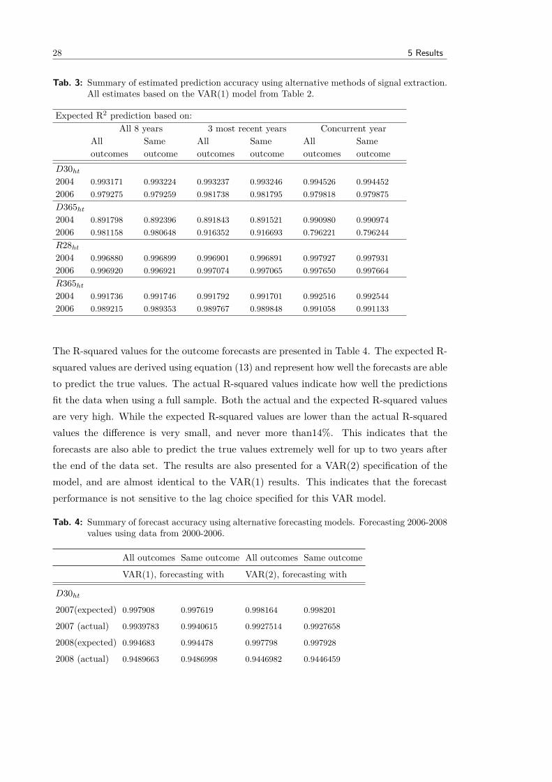
Tab. 3: Summary of estimated prediction accuracy using alternative methods of signal extraction.All estimates based on the VAR(1) model from Table 2.

Expected R2 prediction based on:All 8 years 3 most recent years Concurrent year

Alloutcomes

Sameoutcome

Alloutcomes

Sameoutcome

Alloutcomes

Sameoutcome

D30ht

2004 0.993171 0.993224 0.993237 0.993246 0.994526 0.9944522006 0.979275 0.979259 0.981738 0.981795 0.979818 0.979875D365ht

2004 0.891798 0.892396 0.891843 0.891521 0.990980 0.9909742006 0.981158 0.980648 0.916352 0.916693 0.796221 0.796244R28ht

2004 0.996880 0.996899 0.996901 0.996891 0.997927 0.9979312006 0.996920 0.996921 0.997074 0.997065 0.997650 0.997664R365ht

2004 0.991736 0.991746 0.991792 0.991701 0.992516 0.9925442006 0.989215 0.989353 0.989767 0.989848 0.991058 0.991133

The R-squared values for the outcome forecasts are presented in Table 4. The expected R-squared values are derived using equation (13) and represent how well the forecasts are ableto predict the true values. The actual R-squared values indicate how well the predictionsfit the data when using a full sample. Both the actual and the expected R-squared valuesare very high. While the expected R-squared values are lower than the actual R-squaredvalues the difference is very small, and never more than14%. This indicates that theforecasts are also able to predict the true values extremely well for up to two years afterthe end of the data set. The results are also presented for a VAR(2) specification of themodel, and are almost identical to the VAR(1) results. This indicates that the forecastperformance is not sensitive to the lag choice specified for this VAR model.

Tab. 4: Summary of forecast accuracy using alternative forecasting models. Forecasting 2006-2008values using data from 2000-2006.

All outcomes Same outcome All outcomes Same outcome

VAR(1), forecasting with VAR(2), forecasting with

D30ht

2007(expected) 0.997908 0.997619 0.998164 0.998201

2007 (actual) 0.9939783 0.9940615 0.9927514 0.9927658

2008(expected) 0.994683 0.994478 0.997798 0.997928

2008 (actual) 0.9489663 0.9486998 0.9446982 0.9446459

5.2 Hip Replacement 29


D365ht

2007(expected) 0.973235 0.971065 0.979825 0.979843

2007 (actual) 0.9774626 0.9764693 0.9616151 0.9613662

2008(expected) 0.968023 0.96491 0.976735 0.979905

2008 (actual) 0.9759809 0.9745514 0.9708943 0.9708727

R28ht

2007(expected) 0.97878 0.979752 0.993951 0.992514

2007 (actual) 0.9911799 0.9912462 0.9912541 0.9912401

2008(expected) 0.924943 0.912794 0.953368 0.957072

2008 (actual) 0.993593 0.9936331 0.9943355 0.9943442

R365ht

2007(expected) 0.890177 0.890824 0.895657 0.867804

2007 (actual) 0.9843904 0.9845041 0.9845231 0.9842737

2008(expected) 0.846979 0.84891 0.828721 0.841011

2008 (actual) 0.980951 0.981266 0.9836124 0.9833608

5.2 Hip Replacement

The parameter estimates of the basic model run for Hip Replacement are presented inTable 5. The estimates suggest that D365ht is persistent over time, but that the otherquality indicators being considered are not. The lag coefficient of D365ht is almost 0.6,as compared to lag coefficients of about 0.2 for R28ht and R365ht, and about 0.01 forD30ht. The variance of initial conditions indicates a standard deviation of about 2%across hospitals for D30ht, 3% for R28ht, 4% for D365ht and 5% for R365ht. Similarlythe variance of their residuals shows an annual standard deviation of 1% for D30ht andD365ht, 3% for R28ht and 4% for R365ht. The correlation coefficients amongst indicators,and amongst residuals, indicate a high positive correlation between R365ht and R28ht,and a weak positive correlation between D30ht and D365ht. There is a positive correlationbetween the residuals of D365ht and R28ht, while the correlation coefficient amongst thesetwo indicators in the year 2000 is low and negative. The opposite is true for the pairD365ht and R365ht which have a negative correlation in the year 2000, but a low positivecorrelation between their residuals. Finally there is a positive correlation between D30ht

and R28ht.

30 5 Results

Tab. 5: Estimates of Hip Replacement multivariate VAR(1) parameters for hospital specific effects.

D30ht R28ht D365ht R365ht

D30h(t−1) -0.047351 -0.224300 -0.627994 -0.282623

(0.02543) (0.07851) (0.08952) (0.09652)

[-1.86231] [-2.85705] [-7.01536] [-2.92803]

R28h(t−1) -0.030140 0.312121 -0.359189 0.468140

(0.01479) (0.04567) (0.05207) (0.05615)

[-2.03789] [ 6.83480] [-6.89816] [ 8.33795]

D365h(t−1) 0.036579 0.058774 0.633914 -0.029772

(0.00686) (0.02119) (0.02417) (0.02606)

[ 5.32910] [ 2.77313] [ 26.2315] [-1.14255]

R365h(t−1) -0.016563 -0.045723 -0.039086 0.018910

(0.01098) (0.03390) (0.03865) (0.04168)

[-1.50871] [-1.34884] [-1.01124] [ 0.45373]

ResidualsS.D. dependent 0.011466 0.036723 0.049172 0.046638


Correlation of residuals (R28ht) -0.197193 1.000000 0.350683 0.790476

Correlation of residuals (D365ht) 0.262098 0.350683 1.000000 0.149165

Correlation of residuals (R365ht) -0.250718 0.790476 0.149165 1.000000

Initial ConditionsS.D. dependent in 2000 0.019079 0.033392 0.044777 0.046217

Correlation with D30ht in 2000 - 0.3661 0.2470 0.1459

Correlation with R28ht in 2000 0.3661 - -0.1613 0.7196

Correlation with D365ht in 2000 0.2470 -0.1613 - -0.4921

Correlation with R365ht in 2000 0.1459 0.7196 -0.4921 -

Sample (adjusted): 1997 2008Included observations: 1462 after adjustments

Standard errors in ( ) & t-statistics in [ ]

Figure 6 illustrates the signal to noise ratios of the observed hospital outcome measuresagainst the number of Hip Replacement cases treated in each hospital. For Hip Replace-ment, the signal to noise ratios are quite high, indicating that the four outcome measuresare good indicators of hospital performance. Similar to the previous conditions, the signalto noise ratio increases as more cases are included in the analysis, and the differencesbetween the four indicators begin to shrink. Yet, year-long mortality consistently has the


strongest signal of the four conditions, despite not having as high a signal variance as it didfor AMI. While year-long readmissions have a higher signal variance than year-long mor-tality (Table 5), they most probably have higher amounts in the variance of the estimationerror, causing them to perform the worst of the four measures.

Fig. 6: Signal to noise ratio for the four Hip Replacement outcome measures (year 2005) .

Figures 7 – 10 present the filtered Hip outcome measures, their 95% confidence intervalsand the corresponding latent outcome measures derived in Chapter ?? for selected hospi-tals. The sample for Hip Replacement is longer than for AMI, and so all figures presentinformation back to 1996. Similar to the other two conditions, the filtered estimates aresmoothed averages of the latent measures, and the confidence intervals are wider, againdue to a limited number of hospitals available in the data. Also similar to Stroke, thelatent measure for the small hospital, upper left hand corner, is more erratic than forthe medium and large hospitals, thus making the filtered estimates useful in terms ofinterpreting a trend over time.

32 5 Results

Fig. 7: Filtered and latent estimates for Hip Replacement D30ht.

Fig. 8: Filtered and latent estimates for Hip Replacement D365ht.


Fig. 9: Filtered and latent estimates of Hip Replacement R28ht.

Fig. 10: Filtered and latent estimates of Hip Replacement R365ht.

Table 6 indicates the R-squared estimates for the predictions made for the Hip filtered out-comes, using different amounts of past data. The R-squared values for Hip are extremely

34 5 Results

high, indicating a near perfect prediction for all measures, even when using only one yearof data. Table 7 indicates the R-squared values for the outcome forecasts, estimated usingequation (13), and predictions estimated using equation (12). These are also near perfectfor both the forecasts and predictions, and both the VAR(1) and VAR(2) specifications.This indicate that the model is able to forecast estimates as well as it is able to predictthem from a full set of data, regardless of the lag choice specified in the model.

Tab. 6: Summary of estimated prediction accuracy using alternative methods of signal extraction.All estimates based on the VAR(1) model from Table 5.

Expected R2 prediction based on:All 11 years 3 most recent years Concurrent year

Alloutcomes

Sameoutcome

Alloutcomes

Sameoutcome

Alloutcomes

Sameoutcome

D30ht

2004 0.999851 0.999851 0.999850 0.999852 0.999824 0.9998292006 0.999856 0.999852 0.999860 0.999857 0.999840 0.999840D365ht

2004 0.993021 0.992983 0.992833 0.992773 0.998047 0.9980652006 0.994185 0.994248 0.991052 0.990711 0.982275 0.982161R28ht

2004 0.998588 0.998589 0.998595 0.998593 0.998714 0.9987062006 0.997845 0.997845 0.997835 0.997836 0.997967 0.997969R365ht

2004 0.995829 0.995849 0.995807 0.995831 0.996284 0.9962422006 0.993924 0.993940 0.993907 0.993959 0.995122 0.995136

Tab. 7: Summary of forecast accuracy using alternative forecasting models. Forecasting 1996-2008values using data from 1996-2006.


VAR(1), forecasting with VAR(2), forecasting with

D30ht

2007(expected) 0.999837 0.9998281 0.9998208 0.9998139

2007 (actual) 0.9998575 0.9998609 0.9998577 0.9998588

2008(expected) 0.9997321 0.999688 0.9997113 0.9996896

2008 (actual) 0.9998561 0.999858 0.9998613 0.9998624

D365ht

2007(expected) 0.9968599 0.9970006 0.9963497 0.9963019

2007 (actual) 0.9869273 0.9871355 0.9848145 0.9850215

2008(expected) 0.9965712 0.9964086 0.9957694 0.9954451

2008 (actual) 0.9840067 0.9841068 0.9814323 0.9818322

5.3 Comparison of Indicators 35


R28ht

2007(expected) 0.9985577 0.9983832 0.9987864 0.9986095

2007 (actual) 0.9980288 0.998031 0.9980153 0.9980155

2008(expected) 0.9995171 0.9995244 0.999558 0.9995869

2008 (actual) 0.9767528 0.9767398 0.9767273 0.9767253

R365ht

2007(expected) 0.9989753 0.9989704 0.9990094 0.9990171

2007 (actual) 0.9928861 0.9929147 0.9931077 0.993055

2008(expected) 0.999464 0.9994054 0.999514 0.9994828

2008 (actual) 0.9878172 0.9878773 0.9880453 0.9880126

5.3 Comparison of Indicators

In this subsection, we are able to relate our findings to policy by ranking the hospitals inthe AMI sample using three different indicators of performance for the year 2005. Thefirst indicator is an aggregated 30-day mortality rate as available in the raw data. Thesecond performance indicator is the latent 30-day mortality rate, while the third measureis the filtered 30-day mortality rate estimated using the McClellan and Staiger (1999)methodology. The hospitals are also ranked by the other outcomes and these are reportedin Appendix A due to space constraints. The year 2005 is presented as it is in the middleof the sample and allows enough information to construct the filtered measures from,however the R-squared values in the AMI section suggest that even with less data thefiltered measures are still good predictors. The outcomes are ranked only for AMI at notthe other conditions, as the results are very similar and do not provide further insight.

36 5 Results

Tab. 8: Rankings of 2005 AMI D30ht measures.

Ranking Mean D30ht Hospital Latent D30ht Hospital Filtered D30ht Hospital

Top 10

1 0.0521401 55 -8.417754 83 -2.490163 17

2 0.0532544 9 -5.088554 81 -2.113111 54

3 0.0536913 89 -5.00683 42 -1.934144 22

4 0.0594286 119 -4.887803 47 -1.651729 103

5 0.0645161 62 -4.834379 22 -1.651613 3

6 0.0681818 19 -4.648541 15 -1.608179 18

7 0.0681818 97 -4.089908 1 -1.47745 7

8 0.0684932 80 -4.078938 50 -1.438395 107

9 0.0758808 52 -3.924413 16 -1.425196 21

10 0.0774194 42 -3.834195 68 -1.343411 89

Bottom 10

110 0.1702128 12 2.985045 3 0.2998581 33

111 0.1727941 36 3.342186 7 0.3957789 118

112 0.1759531 96 3.580219 41 0.4082001 41

113 0.1787072 17 3.738158 89 0.4182017 99

114 0.19 53 4.557611 90 0.5266839 66

115 0.1901408 71 4.750142 17 0.5433974 38

116 0.1929825 41 5.562703 53 0.5688122 35

117 0.1987578 90 5.586496 71 0.9426492 27

118 0.2 66 18.70218 43 1.04961 9

119 0.3426574 43 28.97059 66 1.091938 56

Table 8 presents the top and bottom 10 hospitals as ranked by the three different perfor-mance measures together with the values of each measure. Each hospital is represented bya number which has been randomly assigned to be its identifier. Figure 11 illustrates thedifferent rankings for the first 15 hospitals in the sample. What is immediately apparentfrom both Table 8 and Figure 11 is that depending on the indicator used the ranking ofhospitals changes substantially, although not always in the same direction. Some hospitalsgo from a very high ranking to a very low ranking. Hospital 9 went from being rankedsecond best to second worst when using the filtered measure to rank performance insteadof the raw aggregated mortality measure. Hospital 3 on the contrary, went from a verylow ranking, 96 to a very high ranking, 5. There are also cases where two measures seemto be more similar to one another, but where rankings stay relatively consistent such as

5.3 Comparison of Indicators 37

hospitals 11 and 15.

Fig. 11: Rankings of 2005 AMI quality measures for D30ht.

Figure 12 presents the full time series of the three different performance indicators forhospitals 3, 9, 11 and 15. This alternative presentation of the data can help to betterunderstand why the rankings are different from one another. In the upper left handcorner the trajectories of hospital 3’s indicators are presented. The mean raw mortalityonly ranges between 0 and 1, as each patient is coded as either having died or survived.When ranked according to this indicator, hospital 3 does relatively poorly coming in 96thout of 119 in 2005. This indicator does not adjust for differences in patient characteristics,such as co-morbidity or deprivation, while the latent measure does. When looking at theperformance of hospital 3 as reported by latent measure there is much more variation fromyear to year. The year 2005 is the worst year in terms of hospital 3’s performance, andthe hospital is ranked 110 of 119. In all other years however, the hospital performs aboveaverage. The third indicator, the filtered measure, is constructed using the informationprovided throughout the time-series and from the other outcome measures. While thefiltered indicator does reflect hospital 3’s worsening performance over time, it smooths outthe year-to-year variation allowing for a more representative overall picture when singlingout one year. The performance ranking for hospital 3 using the filtered measure is 5 outof 119, which is a huge difference from the latent measure but reflects the hospital’s above

38 5 Results

average performance in all the other years.

When looking at hospital 9 in the upper right hand panel, again the raw mortality has muchless variation than the other two indicators. Using this indicator hospital 9 ranks 2nd outof the 119 in 2005. The latent measure adjusts for some of the patient differences throughthe and shows a very different picture of performance, with much larger year to yearvariation. Performance as reported by this indicator starts out much worse than averagein 2000, improving in the years 2001-2006, but worsening again after. In 2005 performanceis still above average, but adjusting patient characteristics, the ranking falls from 2 to 16.The third indicator, the filtered measure, is constructed using the information providedthroughout the time-series and from the other outcome measures. Thus, the improvementin performance is indicated, however not as sharply as by the latent measure, and neverso much that it results in above average performance. This adjustment causes the rankingto drop down to 118.

Fig. 12: AMI D30ht quality indicators for selected hospitals.

Hospital 11 in the bottom right hand panel ranks 79 out of 119 when using the aggre-gated raw mortality measure. However the latent variable indicates that when controllingfor patient characteristics performance varies considerably from year to year, sometimesreaching very high levels above average, and others falling far below average. 2005 is one ofthe years where performance is below average, and thus when ranked according to it does

39

poorly coming 104th out of 119. The filtered indicator by definition provides a smoothedout measure of average performance across time and incorporating the performance of theother outcome measures. This is apparent from the diagram which shows less volatilityover time in the filtered indicator. Using this indicator the ranking falls down to 87th out of119, which lies between the two other measures. Finally, when looking at the performanceof hospital 15 in the bottom right hand panel we see a similar result. The latent measureshows much more erratic performance from year to year once it controls for all the patientcharacteristics, and the filtered measure is able to summarize these into a much smoother,consistent trend.

Overall, the analysis provides support for the following: Aggregate raw measures are un-able to produce a consistent performance ranking of hospitals that controls for systematicdifferences in patients case mix, such as deprivation or severity. The latent measures doadjust explicitly for these differences, but exhibit year-on-year variation and therefore dif-ferent rankings of hospital performance depending on the year selected, making it difficultto draw conclusions on overall hospital performance over time. The filtered measures areable to summarize the information provided by the latent variable over time and considerthe performance of the other indicators alongside it, thus providing a much more consistentpicture of performance.

The largest difference in rankings is observed in hospitals treating fewer patients. Smallcaseload leads to increased volatility in the raw mortality and readmission measures acrossthe years. While the latent measures control for systematic patient differences in hospitals,the volatility due to small numbers remains. This finding was also reported in Papanicolasand McGuire (2011), where latent estimates calculated for small hospitals always had themost erratic performance measures from year to year. The filtered measures are better atsmoothing out the jumps from year to year as they combine all the information from thetime-series and across the other variables. Thus in these cases, the filtered measure willbe a better indication of performance in any one year.

6 Discussion

In their paper The Quality of Health Care Providers, McClellan and Staiger (1999) proposea methodology with which to evaluate health care providers. Their framework is able totackle some of the main limitations inherent to quality measurement, allowing them tocreate indicators which: integrate different dimensions of quality into one measure, reflectthe multifaceted nature of performance; filter out much of the noise inherent to this type of

40 6 Discussion

measure as a result of the small number of patients treated and the large number of factorswhich contribute to outcomes; and to eliminate much of the bias created from systematicdifferences in patient mix which may result in variations in treatment. Their paper uses USpatient level data for elderly American’s suffering from heart disease to create performanceindicators at the hospital level. They are able to prove that the indicators they createpredict and forecast quality remarkably well, better than many existing methods.

Despite its advantages over traditional methods, this analysis has not been applied toevaluate hospitals outside the US3, or for other conditions. This paper attempts to repli-cate their analysis using English patient level data for a wider range of conditions. Thepaper is also able to address some of the limitations acknowledged by the authors, due togaps in their data on patient co-morbidity, which can be used to create even more robustindicators. Our results indicate that this method can be applied to other countries withsimilar data, and when controlling for co-morbidity are able to produce indicators withhigh prediction accuracy. However, in our application of this method to a different settingwe are also able to identify other difficulties, which arise to do a smaller sample of hospitalsavailable in the English data as compared to the US data.

The first step of the methodology, creating latent measures of performance for each of theoutcomes of interest, is presented in Papanicolas and McGuire (2011). These latent mea-sures serve essentially as risk adjusted measures of performance, as they are able to controlfor exogenous patient characteristics such as age, gender, deprivation and co-morbidity.They proved to be useful for detecting trends and comparing hospital performance to theirpeers. When analysed more closely, to see what factors influenced performance, the resultsindicated that many of the indicators are dynamic, and also related to one another. Thispaper replicates the second step of the methodology which uses a VAR framework thatis able to incorporate the time series information, as well as the relationship to other theother outcome variables into new performance indicators. Both the VAR models, and theindicators inform us on the performance of hospitals.

The results of the VAR models indicate which dimensions of hospital performance arepersistent across different conditions, indicate how much they vary across hospitals andover time, and provide insight as to their relationship with each other. The results forall conditions suggest that of the four measures included in the model, year-long mor-tality is the most persistent dimension of performance. In all conditions for which thismethodology was used, it suggested a strong dynamic presence for the year-long mortality

3 It has been applied to evaluate educational outcomes in the USA, for more information see Kane et al.(2002).

41

indicator. For most conditions, except Hip Replacement, this indicator also exhibits ahigh standard deviation across hospitals, ranging from 20% to 5%. The high variationassociated with year-long survival most likely stems from a variety of factors outside theprovider’s influence, such as patient behaviour and lifestyle. Although the extent of thisinfluence will vary by condition.

The persistence of the 30-day mortality indicator varied considerably more by condition,while it was quite low for AMI and Hip Replacement which are the results reported inthis paper. The variation of 30-day mortality across hospitals also varies considerably bycondition, and again was low for AMI, at around 6% and Hip Replacement, at around 1%.Unlike our results, the McClellan and Staiger (1999) paper finds that 30-day mortalityis more persistent than year-long mortality for AMI, and that shorter term mortality ismore persistent than year-long mortality for IHD. This difference could be explained byvariations in the UK and US treatment pathways. It could also be linked to the differentsamples being analysed by the different investigations; their analysis focused only on theelderly while ours examined all patients. It may also be related to the fact that we wereable to adjust for patient co-morbidity which they did not have the data to do.

Similarly, previous analyses using the latent indicators in Papanicolas and McGuire (2011)only identified a significant dynamic relationship between IHD and Hip Replacement foryear-long mortality, and a significant dynamic relationship for AMI, IHD, Stroke and HipReplacement for 30-day mortality. Given the performance of the filtered estimates on thedifferent goodness of fit measures this could be related to the noise in the latent estimateswhich obscure the ‘true’ quality effect. It could also reflect the number of restrictions setin the GMM model, which the VAR model does not apply.

Moreover, we mention in the results section that for this analysis the VAR(1) specificationwas chosen for ease of interpretation and parsimony. However, different specificationswere indicated as marginally better fits for the model by the Aikake and Swartz lag tests.Yet, when tested with alternative specifications the results did not differ substantially.Moreover, the R-squared estimates calculated for a VAR(2) specification, as reported inthe results section, indicate similar results for all conditions, and in many cases do notindicate improved fit. However, investigation for each condition could benefit from theinclusion of more lags to create more robust predictions and forecasts, especially if thereis a longer time-series being analysed.

The readmission indicators are by and large less persistent indicators of quality as com-pared to mortality. The coefficients on the lags of 28-day emergency readmissions range

42 6 Discussion

between 0.4 and 0.5 for AMI and Hip Replacement, while year-long readmissions are notpersistent for either condition. The variation in short and long term readmissions variesmore considerably by condition. The standard deviation on both indicators is around5% for AMI and Hip Replacement but ranges from between 10-2% for some of the otherconditions estimated.

The AMI model indicates a strong positive correlation between 28-day readmissions andyear-long readmissions, and weaker positive correlation between 30-day mortality andyear-long mortality. These associations are expected as they all represent worse outcomes.However, the model also shows a negative association between mortality and readmissionspresent for some conditions and different time combinations, but strongest between year-long mortality and year-long readmissions. McClellan and Staiger (1999) also observe thisresult, for AMI, although for 30-day mortality and year-long readmissions. They notethat while a positive correlation might be expected, as higher values for both indicatorsrepresent worse outcomes, the negative correlation may reflect the relatively poor heartfunction of ‘marginal’ patients who survive when treated in high quality hospitals. Thus,the hospitals which have worse mortality measures will perform better on the readmissionmeasures, as fewer severely ill patients survive to be readmitted. Moreover if healthierpatients led to low mortality rates, than complication rates for that hospital would also belower, thus there are quality differences amongst hospitals which are not linked to patientselection.

The Hip Replacement model suggests mixed association between the readmission andmortality variables; indicating a positive correlation between some of the mortality andreadmission combinations and negative correlations between the others. For example, 30-day mortality is negatively associated with both short and long term readmissions butyear-long mortality has a positive association. In most of the conditions, all associationsare weak. However, for no condition were all associations positive, indicating that oneshould be cautious when interpreting readmission measures in isolation as they may notbe indicative of higher quality. The results of the VAR models also report the correlation ofthe residuals for the different indicators. In all models short term and long term mortalityare positively correlated with one another, although in most cases this is very weak. Shortand long term readmissions have strong positive correlations with each other in the AMIand Hip Replacement models, but very weak associations for most of the other conditions.

The signal variances estimated using the VAR parameters were also used together withthe estimation error to construct signal to noise ratios for each outcome measure in eachcondition for the year 2005. The first striking result is how strong the signal is for the

43

indicators in most conditions, for a sufficient sample of patients. While the number of casesrequired to get a good signal to noise ratio varies by condition, in most cases it includes themedium to large volume hospitals. McClellan and Staiger (1999) also observe this findingin their paper, and note that it is generally harder to observe the true performance ofsmaller hospitals from patient outcome data. This is because the variation in the data willbe more strongly influenced by differences in treatment, such as the presence or absenceof an individual physician, which would have relatively smaller effects in a larger hospital.Moreover, If we consider the average number of cases per hospital (Table 1) together withthe number of cases above which the signal to noise ratio because high enough, we seethat only for hospitals of average size and above do the patient outcome measures for asingle year provide relatively good information on performance.

The other striking result from the signal to noise ratios was that in all cases, except CCF,long-term mortality had the strongest signal. This suggests that for these conditions, thelong term measure of mortality is a more useful measure of quality than the short termmeasure. Similarly, for most conditions year-long readmissions had a stronger signal than28-day readmissions, although this was not the case for Hip Replacement. Indeed 28-dayreadmissions in almost all cases tended to be the worst performing measure. For casessuch as AMI, where treatment variations in the short term have high implications forsurvival, one would expect the short term mortality measure to have a stronger signal.Especially as long term outcomes add more noise. This finding was reported by McClellanand Staiger (1999) in the US analysis. It is interesting that this is not the case in the UKscenarios, and raises interesting questions as to why.

One possibility for the noise found in the short term estimates, may linked to the organiza-tion of the health system and different health policies within in the UK. In the NHS datacollection and reporting has not traditionally been attached to financing as it is in a claimstype system such as that of the US, this may lead more error in estimates if less effortis put into coding. On the other hand, since 2000 many health policies have focused onusing measures such as 30-day in-hospital mortality and 28-day emergency readmissionsto measure and reward the performance of hospitals, such as the star ratings. There hasbeen criticism surrounding these policies and the distortionary results they had on indica-tors, such as manipulation of data collection (Bevan and Hamblin, 2009). In addition, theintroduction of payment by results (2004/5) has now linked coding to hospital paymentschanging the importance of good coding. As a result, discrepancies in coding practiceshave been reported in the literature, such as hospitals coding deaths as palliative care inorder to reduce mortality rates (Hawkes, 2010). Thus, it is plausible that the emphasisput on the short term indicators for policy has created more measurement error in their

44 6 Discussion

collection, making the longer term measures perform better despite the additional noisein them from other exogenous factors such as patient behaviours and/or lifestyles.

The McClellan and Staiger (1999) analysis replicated the VAR models for different samplesof hospitals in order to better understand the differences in estimation parameters betweenthem. We were unable to do this as the number of hospitals in our sample across eachof our conditions were considerably less, at around 100 per condition as opposed to theirsample of approximately 4,000.

While the results of the VAR models prove informative in themselves, they can also beused to create ‘filtered measures’ of each of the four indicators. These filtered estimatesare able to encompass the time-series relationships within indicators, as well as the corre-lations between measures, allowing them to portray a more accurate description of overallperformance. The results section presents these filtered measures together with the latentmeasures in a series of diagrams for each outcome, for each condition. These figures havethree main similarities throughout all conditions. The first is that the filtered indicatorsare able to provide smoother estimates over time as compared to the latent measures whichexhibit considerable year-to-year variation. The second is the wider confidence intervalsof the filtered measures, which are about double the size of the latent measure confidenceintervals. In their analysis, McClellan and Staiger (1999) note that the confidence inter-vals for their filtered estimates are much tighter than those of the latent measures. Weattribute this different finding to the smaller sample of hospitals we used to estimate thefiltered estimates, resulting in higher uncertainty surrounding the estimates4. However,many critiques of the VAR methodology note that the standard errors of the variance de-compositions are large that it is difficult to make inferences about them (Sims, 1980). Inthis instance as well, the wider confidence intervals make it much harder to draw conclusiveinterpretations from the estimates about relative hospital performance.

Finally, the third similarity across conditions in the performance of the estimates for thesmall hospitals. While the filtered estimates smooth out this performance, and have wideconfidence intervals, the latent measure will often lie outside these bounds. This reflectsobservations noted earlier, about predicting performance for small hospitals, which theraw measures are very sensitive to differences in treatment.

An evaluation of the filtered estimates in prediction the variation of true hospital effectsis estimated through R-squared estimates, based on the adapted formula in McClellanand Staiger (1999). The R-square estimates for all filtered measures, in all conditions,

4 Their sample consisted of 3945 hospitals while we had data on around 120 hospitals per condition.

45

are very high, suggesting that the filtered estimates are able to predict true performanceremarkably well. These high estimates are in line with the very high signal to noise ratiosof the original data, discussed previously. Moreover, the R-squared measures also indicatethat the model is also able to predict very accurately using different amounts of data,including that of only one year. The R-squared values presented in this paper are muchhigher than the ones reported byMcClellan and Staiger (1999), especially when using alimited set of data to create predictions. This differs from the McClellan and Staigerresults, where the R-squared estimates decline when a smaller sample is used to constructthe indicators. This is most probably related to differences in the underlying data. Forinstance, unlike them, we had information on patient co-morbidity which allowed us tobetter adjust for case-mix. Also while their sample only considered the elderly we lookedat the entire patient population.

As discussed previously, the VAR structure allows the model to forecast outcomes forfuture years. By using the data to estimate performance the final years of our sample, andcompare these data to the true estimates we are able to assess how well the model forecastsdata. The R-squared results using this formula (equation (13)) were also very high for allconditions, indicating the VAR’s ability to forecast outcomes. While these estimates areagain higher than McClellan and Staiger’s, they also note the model’s ability to forecastextremely well. The results are also presented for a VAR(2) specification of the model, andare almost identical to the VAR(1) results. This indicates that the forecast performanceis not sensitive to the lag choice specified in the VAR model.

The last section of this paper considers how hospitals perform when ranked by the threedifferent measures (raw, latent and filtered). The results are quite striking. Dependingon the measure chosen, hospitals may go from the top of a ranking to the bottom, or theopposite. The hospitals with the fewest cases are most influenced by the type of measure asthere is so more variance in the raw and latent estimates. The filtered measures are betterat smoothing out the jumps from year to year as they combine all the information fromthe time-series and across the other variables. Thus in these cases, the filtered measurewill be a better indication of performance in any one year. The latent estimates, whilerisk adjusted are very erratic from year-to-year, and rankings may change suddenly whenlooking at year snapshots. Raw measures do not control for exogenous characteristics thatinfluence outcomes, and so are the worst measure of the three. While the filtered estimatesare much better at providing a much more consistent picture of performance over time,we do not advocate the ranking of hospitals, as this exercise shows how sensitive rankingsare to the method chosen.

46 6 Discussion

Much of the analysis of this paper focuses on identifying which indicators are more usefulfor comparing performance across hospitals. The VAR models indicate which measuresare more persistent for the different conditions, how much they vary across hospitals,how well they capture the true signal in the data and how they are correlated with theother measures being considered. The results overall suggest exercising caution wheninterpreting any indicator alone as it may be misleading given its relationship with theother outcome measures. However, the mortality indicators capture more of the true signalthan the readmission measures for most conditions, and especially long-term mortalitymaking it a better indicator to look at.

In conclusion, the analysis of the VAR models for the seven conditions chosen indicateconsiderable correlation of the outcomes across time and between measures. The degree ofpersistence varies by measure and across conditions, as does the extent to which measuresvary across hospitals. However, in almost all cases the most persistent measure with thestrongest signal was year-long mortality. Some of the other more generalizable findings arethat predictions are weaker for hospitals with fewer cases, and variation in their outcomesfrom year to year is larger. However, measures overall are very good at identifying the truesignal of good performance in different hospitals. Indeed the R-squared values indicatethat the measures are extremely good predictors and forecasters of performance.

47

A Appendix: Comparison of Indicators

Tab. 9: Rankings of 2005 AMI D365ht measures.

Ranking Mean D365ht Hospital Latent D365ht Hospital Filtered D365ht Hospital

Top 10

1 0.087248 89 -10.9951 83 -3.58184 17

2 0.108949 55 -7.33457 119 -3.03305 54

3 0.113143 119 -7.01737 47 -2.52628 22

4 0.116531 52 -6.30999 42 -2.45368 3

5 0.123737 97 -5.81326 45 -2.3618 103

6 0.129032 62 -5.72524 15 -2.03254 18

7 0.141892 45 -5.43161 80 -2.01344 7

8 0.149923 112 -5.26463 91 -1.99536 107

9 0.150538 88 -4.79057 22 -1.79006 44

10 0.155303 19 -4.63651 62 -1.75694 40

Bottom 10

110 0.27566 21 4.33436 21 0.998402 114

111 0.276094 76 4.432666 90 1.038727 41

112 0.276423 61 4.860979 96 1.257631 38

113 0.285 53 4.952693 53 1.294286 33

114 0.291228 41 4.981547 36 1.342004 35

115 0.29912 96 5.641765 107 1.400486 99

116 0.306338 71 7.110268 10 1.55153 66

117 0.312139 3 7.266694 3 2.121651 27

118 0.4 66 7.715625 71 2.203174 9

119 0.426573 43 18.70868 43 2.538532 56

Tab. 10: Rankings of 2005 AMI R28ht measures.

Ranking Mean R28ht Hospital Latent R28ht Hospital Filtered R28ht Hospital

Top 10

1 0 66 -17.15334 66 -0.5097684 56

2 0.0410959 80 -13.77112 83 -0.4249609 27

3 0.0537634 62 -9.429364 62 -0.4037885 9

4 0.0758123 57 -7.974833 80 -0.3244067 38

5 0.0769231 43 -6.535955 43 -0.2796607 99

48 A Appendix: Comparison of Indicators


6 0.0824373 88 -4.354861 57 -0.2724753 41

7 0.0873786 113 -3.504739 113 -0.2207526 116

8 0.09375 36 -3.356516 36 -0.2168493 33

9 0.0989209 63 -2.987282 88 -0.1949843 35

10 0.0990415 51 -2.770071 45 -0.1943502 53

Bottom 10

110 0.1564246 85 3.137839 23 0.5282587 83

111 0.1594203 27 3.158059 6 0.5671023 107

112 0.1598916 14 3.614229 27 0.5836549 106

113 0.1601423 23 3.619557 72 0.589515 40

114 0.1606061 16 3.697118 9 0.5981762 3

115 0.1615721 59 4.066902 14 0.6017366 18

116 0.164486 6 4.984622 46 0.7226745 22

117 0.1715976 9 5.005144 16 0.7290823 103

118 0.1856061 19 5.010148 19 0.8328696 17

119 0.1933962 46 5.822222 59 0.8452681 54

Tab. 11: Rankings of 2005 AMI R365ht measures.


Top 10

1 0.118881 43 -12.698 43 -0.6166016 56

2 0.167785 89 -12.05263 83 -0.5771485 33

3 0.169675 57 -7.481782 62 -0.4943517 99

4 0.172043 62 -7.190022 89 -0.483924 38

5 0.172524 51 -5.687592 113 -0.4257711 116

6 0.181004 88 -5.204206 33 -0.3740641 9

7 0.182222 99 -4.925087 99 -0.3105961 62

8 0.18932 113 -4.808173 51 -0.2949201 66

9 0.197425 33 -4.342741 88 -0.2844733 41

10 0.200557 102 -4.314243 58 -0.2767854 118

Bottom 10

110 0.278986 27 4.798292 95 0.4114325 5

111 0.280397 78 4.828352 28 0.4298307 67

112 0.283951 72 4.928086 80 0.4988003 3

113 0.284734 95 5.156519 72 0.5044565 50

49


114 0.285266 86 5.201916 23 0.5073113 77

115 0.288256 23 5.52123 71 0.5493379 18

116 0.292254 71 5.75459 11 0.5793964 17

117 0.292553 11 5.975807 4 0.6079986 40

118 0.301887 46 7.396799 46 0.6340984 106

119 0.4 66 19.4526 66 0.6462436 54

50 A Appendix: Comparison of Indicators

REFERENCES 51

References

Aylin, P., A. Bottle, and A. Majeed (2007, May). Use of administrative data orclinical databases as predictors of risk of death in hospital: comparison of models.BMJ 334 (7602), 1044.

Benbassat, J. and M. Taragin (2000, April). Hospital readmissions as a measure of qualityof health care: Advantages and limitations. Arch Intern Med 160 (8), 1074–1081.

Bentler, P. M. (1980, January). Multivariate analysis with latent variables: Causal mod-eling. Annual Review of Psychology 31 (1), 419–456.

Bevan, G. and R. Hamblin (2009, January). Hitting and missing targets by ambulanceservices for emergency calls: effects of different systems of performance measurementwithin the UK. Journal of the Royal Statistical Society: Series A (Statistics in Soci-ety) 172 (1), 161–190.

Birkmeyer, J. D., J. B. Dimick, and D. O. Staiger (2006, March). Operative mortalityand procedure volume as predictors of subsequent hospital performance. Annals ofSurgery 243 (3), 411–417. PMID: 16495708 PMCID: 1448928.

Birkmeyer, J. D., A. E. Siewers, E. V. A. Finlayson, T. A. Stukel, F. L. Lucas, I. Batista,H. G. Welch, and D. E. Wennberg (2002). Hospital volume and surgical mortality inthe united states. New England Journal of Medicine 346 (15), 1128–1137.

Bloom, N., C. Propper, S. Seiler, and J. V. Reenen (2010, May). The impact of competitionon management quality: Evidence from public hospitals. National Bureau of EconomicResearch Working Paper Series No. 16032.

Brook, R. H., M. E. A., and P. D. Cleary (1996, September). Measuring quality of care— NEJM. New England Journal of Medicine 335 (13), 966–970.

Capewell, S., C. E. Morrison, and J. J. McMurray (1999, April). Contribution of moderncardiovascular treatment and risk factor changes to the decline in coronary heart diseasemortality in scotland between 1975 and 1994. Heart 81 (4), 380 –386.

Charlson, M. E., P. Pompei, K. L. Ales, and C. R. MacKenzie (1987). A new method ofclassifying prognostic comorbidity in longitudinal studies: development and validation.Journal of Chronic Diseases 40 (5), 373–383. PMID: 3558716.

Christiansen, C. L. and C. N. Morris (1997, October). Improving the statistical approachto health care provider profiling. Annals of Internal Medicine 127 (2), 764 –768.

52 REFERENCES

Cohen, P., J. Cohen, J. Teresi, M. Marchi, and C. N. Velez (1990, June). Problemsin the measurement of latent variables in structural equations causal models. AppliedPsychological Measurement 14 (2), 183 –196.

Dimick, J. and H. Welch (2008, January). The zero mortality paradox in surgery. Journalof the American College of Surgeons 206 (1), 13–16.

Dimick, J. B., H. G. Welch, and J. D. Birkmeyer (2004). Surgical mortality as an indicatorof hospital quality. JAMA: The Journal of the American Medical Association 292 (7),847 –851.

Donabedian, A. (1966, July). Evaluating the quality of medical care. The Milbank Memo-rial Fund Quarterly 44 (3), 166–206. ArticleType: research-article / Issue Title: Part2: Health Services Research I. A Series of Papers Commissioned by the Health Ser-vices Research Study Section of the United States Public Health Service. Discussed ata Conference Held in Chicago, October 15-16, 1965 / Full publication date: Jul., 1966/ Copyright © 1966 Milbank Memorial Fund.

Donabedian, A. (1988, September). The quality of care. how can it be assessed? JAMA:The Journal of the American Medical Association 260 (12), 1743–1748. PMID: 3045356.

Enders, W. (2004). Applied econometric time series. J. Wiley.

Fitzpatrick, R. (2009). Patient-reported outcome measures and performnce measurement.In Performance Measurement for Health System Improvement: Experiences, Challengesand Prospects. Cambridge: Cambridge University Press.

Gil, M., J. Marrugat, J. Sala, R. Masia, R. Elosua, X. Albert, A. Pena, J. Vila, M. Pavesi,and G. Perez (1999, April). Relationship of therapeutic improvements and 28-Day casefatality in patients hospitalized with acute myocardial infarction between 1978 and 1993in the REGICOR study, gerona, spain. Circulation 99 (13), 1767–1773.

Hawkes, N. (2010, April). Patient coding and the ratings game. BMJ 340 (apr23 2),c2153–c2153.

Iezzoni, L. I. (1994, December). Using risk-adjusted outcomes to assess clinical prac-tice: An overview of issues pertaining to risk adjustment. The Annals of ThoracicSurgery 58 (6), 1822–1826.

Iezzoni, L. I. (2003, June). Risk adjustment for measuring health care outcomes. HealthAdministration Press.

REFERENCES 53

Iezzoni, L. I., A. S. Ash, M. Shwartz, J. Daley, J. S. Hughes, and Y. D. Mackiernan (1996,October). Judging hospitals by severity-adjusted mortality rates: the influence of theseverity-adjustment method. Am J Public Health 86 (10), 1379–1387.

Jarman, B., S. Gault, B. Alves, A. Hider, S. Dolan, A. Cook, B. Hurwitz, and L. I. Iezzoni(1999, June). Explaining differences in english hospital death rates using routinelycollected data. BMJ 318 (7197), 1515 –1520.

Kane, T. J., D. O. Staiger, D. Grissmer, and H. F. Ladd (2002, January). Volatility inschool test scores: Implications for Test-Based accountability systems. Brookings Paperson Education Policy (5), 235–283. ArticleType: research-article / Full publication date:2002 / Copyright © 2002 The Brookings Institution.

Kessler, D. and M. McClellan (1996, May). Do doctors practice defensive medicine? TheQuarterly Journal of Economics 111 (2), 353 –390.

Kessler, D. P. and M. B. McClellan (2011, April). Is hospital competition socially waste-ful?*. Quarterly Journal of Economics 115 (2), 577–615.

Khush, K., A. Kopelnik, P. Tung, N. Banki, M. Dae, M. Lawton, W. Smith, B. Drew,E. Foster, and J. Zaroff (2005, February). Age and aneurysm position predict patternsof left ventricular dysfunction after subarachnoid hemorrhage. Journal of the AmericanSociety of Echocardiography 18 (2), 168–174.

Klazinga, N. (2011). Health service outcomes. In Health system perfomrance compari-son: an agenda for policy, information and research. European Observatory on HealthSystems and Policies.

Landrum, M. B., S. E. Bronskill, and S. T. Normand (2000). Analytic methods for con-structing Cross-Sectional profiles of health care providers. Health Services and OutcomesResearch Methodology 1 (1), 23–47.

Lilford, R. and P. Pronovost (2010, April). Using hospital mortality rates to judge hospitalperformance: a bad idea that just won’t go away. BMJ 340 (apr19 2), c2016–c2016.

Lilford, R. J., C. A. Brown, and J. Nicholl (2007, September). Use of process measuresto monitor the quality of clinical practice. BMJ : British Medical Journal 335 (7621),648–650. PMID: 17901516 PMCID: 1995522.

Lingsma, H., E. Steyerberg, M. Eijkemans, D. Dippel, W. S. O. Reimer, H. V. Houwelin-gen, and T. N. S. S. Investigators (2010, February). Comparing and ranking hospitalsbased on outcome: results from the netherlands stroke survey. QJM 103 (2), 99 –108.

54 REFERENCES

Lisa I Iezzoni, L. Risk adjustment for performance measurement. In Performance Mea-surement for Health System Improvement: Experiences, Challenges and Prospects. Cam-bridge: Cambridge University Press.

McClellan, M. and D. Staiger (1999, August). The quality of health care providers. Na-tional Bureau of Economic Research Working Paper Series No. 7327. published as Mc-Clellan, Mark and Douglas Staiger. "Comparing The Quality Of Health Care Providers,"Forum for Health Economics and Policy, 2000, v3, Article 6. Mark McClellan & Dou-glas Staiger, 2000. "Comparing the Quality of Health Care Providers," NBER Chapters,in: Frontiers in Health Policy Research, Volume 3, pages 113-136 National Bureau ofEconomic Research, Inc.

McGovern, P. G., D. R. Jacobs, E. Shahar, D. K. Arnett, A. R. Folsom, H. Blackburn,and R. V. Luepker (2001, July). Trends in acute coronary heart disease mortality,morbidity, and medical care from 1985 through 1997 : The minnesota heart survey.Circulation 104 (1), 19–24.

Mohammed, M. A., J. J. Deeks, A. Girling, G. Rudge, M. Carmalt, A. J. Stevens, and R. J.Lilford (2009). Evidence of methodological bias in hospital standardised mortality ratios:retrospective database study of english hospitals. BMJ : British Medical Journal 338.PMID: 19297447 PMCID: 2659855.

Moulton, B. R. (1990). An illustration of a pitfall in estimating the effects of aggregatevariables on micro unit. The Review of Economics and Statistics 72 (2), 334–38.

Normand, S. T., M. E. Glickman, and C. A. Gatsonis (1997). Statistical methods forprofiling providers of medical care: Issues and applications. Journal of the AmericanStatistical Association 92 (439), 803–814. ArticleType: research-article / Full publicationdate: Sep., 1997 / Copyright © 1997 American Statistical Association.

Normand, S. T., R. E. Wolf, J. Z. Ayanian, and B. J. McNeil. Assessing the accuracy ofhospital clinical performance measures. Medical Decision Making 27 (1), 9 –20.

Papanicolas, I. and A. McGuire (2011, May). Using a latent variable approach to measurethe quality of english NHS hospitals. Technical Report 21, London School of Economics,London.

Powell, A. E., H. T. O. Davies, and R. G. Thomson (2003, April). Using routine com-parative data to assess the quality of health care: understanding and avoiding commonpitfalls. Quality and Safety in Health Care 12 (2), 122 –128.

REFERENCES 55

Propper, C., S. Burgess, and D. Gossage (2008, January). Competition and quality:Evidence from the NHS internal market 1991–9*. The Economic Journal 118 (525),138–170.

Propper, C., S. Burgess, and K. Green (2004, July). Does competition between hospitalsimprove the quality of care?: Hospital death rates and the NHS internal market. Journalof Public Economics 88 (7-8), 1247–1272.

Reerink, E. (1990). Defining quality of care: Mission impossible? International Journalfor Quality in Health Care 2 (3-4), 197 –202.

Shahian, D. M., R. E. Wolf, L. I. Iezzoni, L. Kirle, and S. T. Normand (2010, December).Variability in the measurement of hospital-wide mortality rates. New England Journalof Medicine 363 (26), 2530–2539.

Shen, Y. (2003, March). The effect of financial pressure on the quality of care in hospitals.Journal of Health Economics 22 (2), 243–269.

Shojania, K. G. and A. J. Forster (2008, November). Hospital standardized mortalityratios. CMAJ 179 (10), 1037.

Silber, J. H., P. R. Rosenbaum, and R. N. Ross (1995, March). Comparing the contribu-tions of groups of predictors: Which outcomes vary with hospital rather than patientcharacteristics. Journal of the American Statistical Association 90 (429), 7–18. Article-Type: research-article / Full publication date: Mar., 1995 / Copyright © 1995 AmericanStatistical Association.

Sims, C. A. (1980, January). Macroeconomics and reality. Econometrica 48 (1), 1–48.ArticleType: research-article / Full publication date: Jan., 1980 / Copyright © 1980The Econometric Society.

Spiegelhalter, D. J., P. Aylin, N. G. Best, S. J. W. Evans, and G. D. Murray (2002,June). Commissioned analysis of surgical performance using routine data: lessons fromthe bristol inquiry. Journal of the Royal Statistical Society: Series A (Statistics inSociety) 165 (2), 191–221.

Stock, J. H. and M. W. Watson (2001, October). Vector autoregressions. The Journal ofEconomic Perspectives 15 (4), 101–115. ArticleType: research-article / Full publicationdate: Autumn, 2001 / Copyright © 2001 American Economic Association.

56 REFERENCES

Terris, Darcey, D. and C. Aron, David (2009). Attribution and causality in health-care per-formance measurement. In Performance Measurement for Health System Improvement:Experiences, Challenges and Prospects. Cambridge: Cambridge University Press.

Theunissen, N. C. M., T. G. C. Vogels, H. M. Koopman, G. H. W. Verrips, K. A. H.Zwinderman, S. P. Verloove-Vanhorick, and J. M. Wit (1998, July). The proxy problem:child report versus parent report in health-related quality of life research. Quality ofLife Researchs 7 (5), 387–397.

Titterington, D., A. Smith, and U. Makov (1985). Statistical Analysis of Finite MixtureDistributions. John Wiley.

Wooldridge, J. M. (2002). Econometric analysis of cross section and panel data. MITPress.

Wright, J. and K. G. Shojania (2009, March). Measuring the quality of hospital care.BMJ 338 (mar18 2), b569–b569.

For further information on this or any of the

Health publications contact:

Naho Ollason

Managing Editor

LSE Health

The London School of Economics and Political Science

Houghton Street

London WC2A 2AE

Tel: + 44 (0)20 7955 3733

Fax: + 44 (0)20 7955 6090

Email: [email protected]

Website: www.lse.ac.uk/collections/LSEHealth/


Using a latent variable approach to measurethe quality of English NHS hospitals

Working paper No: 21/2011 May 2011 LSE Health

Date post:	27-Apr-2018
Category:	Documents
Upload:	phungtruc
View:	216 times
Download:	3 times

Using a Vector Autoregression Framework to measure … Library Cataloguing in Publication Data A...

Documents