AUTHORS

Peter Bretan � Badleys, North Beck House,North Beck Lane, Hundleby, Spilsby, Lincoln-shire, PE23 5NB, United Kingdom;pete@badleys.co.uk

Peter Bretan received a B.Sc. degree (withhonors) from Kingston University in 1981,followed by a Ph.D. in structural geology fromImperial College, London. Before joining Bad-leys in 1995, he worked as a research geologistand seismic interpreter with the Fault AnalysisResearch Group at Liverpool University. AtBadleys, his main tasks include softwaretraining, technical support, and consulting.

Graham Yielding � Badleys, North BeckHouse, North Beck Lane, Hundleby, Spilsby,Lincolnshire, PE23 5NB, United Kingdom

Graham Yielding received a B.A. degree innatural sciences from Cambridge Universityin 1979, followed by a Ph.D. in geophysics in1984. He then worked for Britoil in Glasgowas a seismic interpreter before joining Badleysin 1988. His current interests include fault-seal analysis, fault populations, and fractureprediction.

Helen Jones � Badleys, North Beck House,North Beck Lane, Hundleby, Spilsby, Lincoln-shire, PE23 5NB, United Kingdom

Helen Jones joined Badleys in 1989. Havingoriginally trained, worked, and published asa biologist, Helen then swapped sciences togeology to provide technical research and sup-port to ongoing project work. In addition, she isthe author of the manuals and online docu-mentation for the TrapTester/FAPS software.

ACKNOWLEDGEMENTS

The authors are grateful to Stephen Dee andPeter Boult for their comments on earlyversions of this manuscript. Laurel Goodwin,Fred Dula, Russell Davies, and Jim Handschyare thanked for their constructive reviews.

Using calibrated shale gougeratio to estimate hydrocarboncolumn heightsPeter Bretan, Graham Yielding, and Helen Jones

ABSTRACT

Fault-zone composition, estimated using the shale gouge ratio (SGR)

algorithm, can be empirically calibrated with pressure data to de-

fine depth-dependent seal-failure envelopes relating SGR to fault-

zone capillary entry pressure (FZP) by the equation: FZP (bar) =

10 (SGR/27 � C). C is 0.5 for burial depths less then 3.0 km (�9850 ft), Cis 0.25 for burial depths between 3.0 and 3.5 km (�9850–11,500 ft),

and C is 0 where the burial depth exceeds 3.5 km (�11,500 ft).

The seal-failure envelope provides a method to estimate the

maximum height of a hydrocarbon column that can be supported by

the fault. Leakage of hydrocarbons across a fault occurs when the

buoyancy pressure exceeds the capillary entry pressure of the fault

and is not confined to the crest of the structure or even to where the

SGR value is lowest.

Established calibration diagrams based on across-fault pressure

differences have overgeneralized the relationship between increas-

ing SGR and increasing pressure support. Calibration diagrams

based on buoyancy pressure show that gas and oil data exhibit a

correlation between increasing SGR and increasing buoyancy pres-

sure but only between SGR values of 20 and 40%. No increase in the

strength of a seal is present, as reflected by an increase in maximum

supportable buoyancy pressure, at SGR values greater than about

40% for both gas and oil data. Column heights do not continue to

increase in the SGR range 50–100%.

Estimating hydrocarbon column heights using seal attributes

depends upon the geologic input to the model, in particular, pres-

sure data, volumetric shale fraction, and the precision of the three-

dimensional mapping of reservoir geometry in the vicinity of the fault.

INTRODUCTION

Fault-seal analysis is a technique for risk assessment of the sealing

and nonsealing potential of faults in petroleum reservoirs. A meth-

Copyright #2003. The American Association of Petroleum Geologists. All rights reserved.

Manuscript received November 19, 2001; provisional acceptance May 7, 2002; revised manuscriptreceived June 27, 2002; final acceptance August 1, 2002.

DOI:10.1306/08010201128

AAPG Bulletin, v. 87, no. 3 (March 2003), pp. 397–413 397

odology for predicting fault-seal behavior in mixed clas-

tic sequences in areas of low differential stress has been

well documented in recent years (e.g., Bouvier et al.,

1989; Jev et al., 1993; Childs et al., 1997; Fulljames

et al., 1997; Knipe, 1997; Naruk and Handschy, 1997;

Yielding et al., 1997, 1999; Knipe et al., 1998).

An essential element of the fault-seal analysis meth-

odology is to calibrate the fault-seal attribute, taken as a

proxy for fault-zone composition, at faults where the

sealing behavior can be demonstrated using pressure

data from wells on either side of the fault (e.g., Fristad

et al., 1997; Yielding et al., 1997). These studies derive

an empirical relationship between fault-seal attribute

values and across-fault pressure information that is used

as a predictor of seal integrity in undrilled fault traps

(e.g., Yielding et al., 1997; Yielding, 2002).

The basis for the calibration is the observation that

many faults in petroleum reservoirs are membrane or

capillary seals (e.g., Schowalter, 1979;Watts, 1987,Grauls

et al., 2002). In a hydrocarbon-water system, leakage of

hydrocarbons through a water-wet fault zone is by cap-

illary action. Leakage of hydrocarbons through the fault

zone takes place when the difference in pressure between

the water and hydrocarbon phases (buoyancy pressure)

exceeds the pressure required for hydrocarbons to enter

and pass through the largest interconnected pore throat

in the seal (displacement or capillary entry pressure).

The driving force for capillary leakage in water-wet fault

rocks is the pressure of the hydrocarbon phase (Bjorkum

et al., 1998; see also Rodgers, 1999 for discussion).

Given that the calibration of fault-seal attributes is a

crucial step in a fault-seal analysis workflow, it is

surprising that there are relatively few accounts that

describe how the predicted fault-seal attributes are

calibrated (e.g., Fristad et al., 1997). Most works

simply note a specific seal attribute value that is able

to support a specific pressure difference (e.g., Bouvier

et al., 1989; Welbon et al., 1997; Ottesen Ellevset et al.,

1998; Childs et al., 2002). The details of the calibra-

tion (e.g., which hydrocarbon phases are juxtaposed),

depth of burial and data used have generally not been

completely documented.

In hydrocarbon exploration, the aim of calibrating

fault-seal attributes is to predict the hydrocarbon col-

umn height in prospects. Several works have described

methods for estimating the height of a hydrocarbon

column (e.g., Berg, 1975; Schowalter, 1979; Jennings,

1987; Watts, 1987; Firoozabadi and Ramey, 1988;

Vavra et al., 1992; Heum, 1996; Ingram et al., 1997;

Bjorkum et al., 1998; Fisher et al., 2001; Childs et al.,

2002). The methods relate the size (radii) of pore

throats in a seal rock, the interfacial tension between

water and hydrocarbons, and the pressure differentials

caused by buoyancy forces. Lateral variations in res-

ervoir juxtaposition geometry, fault-zone property, and

strength of the seal are commonly assumed to be ho-

mogeneous along the entire length of the fault (e.g.,

Fisher et al., 2001). The methods tend to predict that

across-fault leakage will occur at the crest of the

structure where the pressure difference between the

hydrocarbons and water (buoyancy pressure) will be

highest. Ultimately, these deterministic methods re-

quire an estimate for the size of the pore throats in

fault zones and the interfacial tension of oil to water

at reservoir conditions (Jennings, 1987; O’Connor,

2000), which are generally not known in most ex-

ploration settings. Alternatively, in a very simplistic

analysis, the height of a hydrocarbon column is com-

monly estimated by simply assuming the closure is

filled down to the lowest mapped structural or strat-

igraphic spillpoint.

The aim of this contribution is to develop an em-

pirical method to estimate hydrocarbon column heights

using calibrated fault-seal attributes. We describe how

fault-seal attributes, in particular shale gouge ratio

(SGR), can be calibrated using preproduction pressure

data to derive an estimate for the capillary entry pres-

sure of a fault zone. In this context, the pore-throat size

in a fault zone controls capillary entry pressure. In gen-

eral, the smaller the pore-throat size, the higher the

capillary entry pressure required for the seal to fail, and

the greater the hydrocarbon column that can potentially

be supported. The established calibration of fault-seal

attribute data against across-fault pressure differences

(AFPD) is strongly dependent upon which fluid types

are juxtaposed at the fault surface (e.g., oil against water

or gas against water), the depth of burial, and the esti-

mate of the clay content of the fault zone. A large fault

database is used in which all the faults are extensional

normal faults developed in mixed clastic sequences.

The faults were analyzed using the FAPS software

(Freeman et al., 1998 and Yielding et al., 1999 for

details of the methodology).

CALIBRATION OF SHALE GOUGE RATIO BYACROSS-FAULT PRESSURE DIFFERENCE

The primary control on the seal behavior of faults un-

der static pressure conditions is likely to be the clay

content of the fault zone (Yielding et al., 1997; Knipe

398 Using Calibrated Shale Gouge Ratio to Estimate Hydrocarbon Column Heights

et al., 1998; Yielding, 2002). Therefore, an assessment

of the clay content of the fault zone is necessary to

predict the likely entry pressure for hydrocarbons.

Algorithms can be used to predict fault-zone rock type

by considering the amount of clay material that may

have been entrained into the fault zone as a result of the

mechanical processes of faulting (Bouvier et al., 1989;

Jev et al., 1993; Fulljames et al., 1997; Yielding et al.,

1997; Ottesen Ellevset et al., 1998). The algorithm is

then empirically calibrated by testing it at the bounding

faults of hydrocarbon traps.

One such algorithm that is widely used in calibra-

tion studies is SGR (Yielding et al., 1997; Ottesen

Ellevset et al., 1998; Yielding, 2002; see also Freeman

et al., 1998 for definition). Calibration studies using

alternative fault-seal attributes, such as Clay Smear Po-

tentia, or CSP, have been described (e.g., Bouvier et al.,

1989; Jev et al., 1993; Fulljames et al., 1997) but are

more qualitative compared to calibrations using the

SGR algorithm.

The key input for the SGR algorithm is the vol-

umetric shale fraction (V shale) of the intervals adjacent

to the fault. The V shale parameter is a derived product,

typically from gamma-ray or neutron-density logs, and

is commonly used as a general term to describe the

output from a petrophysicist’s interpretation of the

mineralogical content in a suite of well logs. The V shale

parameter is not necessarily the same as the actual

volumetric clay content (Vclay or % phyllosilicates) of

the rock. Detailed analysis of thin sections by point

counting or by x-ray diffraction analysis is required to

determine the true volume clay content, which is seldom

carried out on cores from exploration wells. In terms of

capillary trapping, the size of the pore-throat radius

inversely governs the displacement pressures. As the

pore-throat radius is controlled by the sizes of the

mineral grains and clasts, the critical factor is whether

the presence of fine-grained material can reduce the

pore-throat sizes. Because phyllosilicate minerals are

particularly fine grained, they are most likely to be the

dominant host rock contribution to fault-seal develop-

ment. In this contribution, we use the term SGR as an

estimate of the upscaled phyllosilicate content of the

fault zone.

Seal attributes, such as SGR, must be calibrated

with in-situ pressure data to derive a measure for the

‘‘strength’’ of the seal, and hence hydrocarbon column

height (e.g., Yielding et al., 1997; Yielding, 2002). Ide-

ally, SGR values should be calibrated against the dif-

ference in pressure between the hydrocarbons trapped

at the fault and water in the fault zone (Fristad et al.,

1997; Fisher et al., 2001). However, it is generally not

possible to collect accurate pressure data for water in a

fault zone. The difference in pressure can be obtained

either by measuring the pressure difference between

the hydrocarbon and water phases in the same reservoir

or by measuring the difference in pressure across the

fault (Fristad et al., 1997).

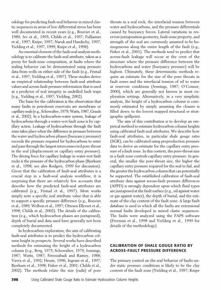
We define AFPD as the observed difference between

in-situ pressure values at a fault surface measured at

the same depth in the upthrown and downthrown sides

of a fault (Figure 1). Pressure-depth data points obtained

from repeat formation tests (RFT) provide the primary

observational measurements of subsurface pressure re-

gimes. Because we are concerned with the absolute pres-

sure difference between the hydrocarbon and the water

phases, values of AFPD are always expressed as positive

values. This definition of AFPD assumes that the fault-

zone material supports the difference in pressure be-

tween the upthrown and downthrown sides of a fault.

It is also assumed that the aquifer across the fault has

Bretan et al. 399

Figure 1. Across-fault pressure difference, or AFPD, is thedifference in pressure between hydrocarbons in the upthrownside (A) and water in the downthrown side (A0) measured atthe same depth on the fault surface. Where there is a commonaquifer, the AFPD values represent buoyancy pressures.Pressure data at wells are extrapolated along horizontalpressure gradients (hydrostatic conditions) to the fault.

the same pressure as water in the fault zone. Pressure

differences arising from juxtaposed sands with different

capillary properties are not considered.

Several authors have compared seal attribute and

AFPD for sand-on-sand reservoir juxtapositions on

faults (e.g., Jev et al., 1993; Welbon et al., 1997; Fristad

et al., 1997; Yielding et al., 1997). Figure 2 is a com-

pilation plot from Yielding (2002). A bounding line

separates a region of data points derived from sealing

faults and a region devoid of data. This bounding line

has been termed the seal-failure envelope (Yielding et al.,

1997; Yielding, 2002) and shows the maximum AFPD

that can be supported at a given SGR. A feature of the

compilation plot is the apparent systematic increase

in AFPD that can be supported by increasing values

of SGR. The equation defining the seal-failure en-

velope relating SGR to AFPD (in bar; 1 bar = 105 Pa

or 14.5 psi), is

AFPDðbarÞ ¼ 10ðSGR=27�CÞ ð1Þ

At burial depths less than 3.0 km (�9850 ft), C is 0.5.

For burial depths between 3.0 and 3.5 km (�9850–

11,500 ft), C is 0.25. When burial depth exceeds 3.5 km

(�11,500 ft) C is 0.

Data points that lie close to the seal-failure en-

velope represent parts of the fault surface that are ex-

pected to be at or near the capillary entry pressure of

the fault zone at specific fault-zone compositions. Data

points that occur below the seal-failure envelope may

arise from sand-on-sand juxtapositions that occur struc-

turally deeper and lower down in the hydrocarbon col-

umn where pressure differences across the fault are

smaller, or at the same depth on the fault but where the

SGR values are greater. Alternatively, such data may

derive from traps that are ultimately controlled by dip

closure away from the fault instead of fault seal (Yielding

et al., 1997).

The seal-failure envelope in Figure 2 is commonly

used to derive a threshold SGR value that is taken to

represent the onset of fault sealing at a specific fault-

zone composition. An SGR value of about 15–20% is

widely considered to represent the threshold between

nonsealing and sealing behavior of faults in mixed

clastic sequences without diagenetic overprinting (see

Fristad et al., 1997; Yielding et al., 1997; Ottesen

Ellevset et al., 1998; Manzocchi et al., 1999). Yielding

et al. (1997) and Yielding (2002) corroborate this

threshold value and the overall trend of the SGR and

across-fault pressure relationship with capillary entry

and breakthrough pressure data from fault-gouge sam-

ples (Gibson, 1994, 1998). However, as we shall demon-

strate subsequently in this contribution, the general trend

of increasing SGR values supporting increasing pressure

400 Using Calibrated Shale Gouge Ratio to Estimate Hydrocarbon Column Heights

Figure 2. Calibration plot of shalegouge ratio against across-fault pressuredifferences for sand-on-sand reservoirjuxtapositions from a variety of fault datasets worldwide (from Yielding, 2002, re-printed with permission from Elsevier).Data are color coded by burial depth: lessthan 3.0 km (�9850 ft) dark blue; 3.0–3.5 km (�9850–11,500 ft) red; 3.5–5.5 km(�11,500–18,050 ft) green. Dashed linesare ‘‘seal-failure envelopes’’ that representthe maximum capillary entry pressure thatcan be supported at a specific SGR value.

differences at the fault may be less well defined than

the compilation shown in Figure 2 appears to suggest.

EMPIRICAL METHOD TO ESTIMATEHYDROCARBON COLUMN HEIGHTS

The empirical relationship between the fault-zone

composition (SGR) and the capillary entry pressure of

the fault zone (AFPD) can be used to derive the

potential hydrocarbon column heights that each part of

the fault may be able to support (Childs et al., 2002).

First, SGR values are calibrated, using equation 1 or

similar equations, to derive the maximum supportable

pressure (taken to be equivalent to capillary entry pres-

sure) along the fault plane. Second, density data for wa-

ter, oil, or gas phases at reservoir conditions are in-

corporated to translate the pressure difference (derived

from the SGR) into the maximum potential hydro-

carbon column height using equation 2 (e.g., Jennings,

1987; Schowalter, 1979):

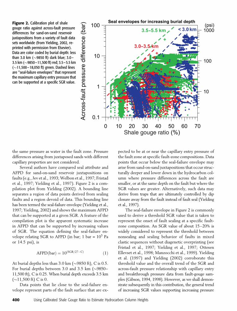
H ¼ dP=gðrw � rhÞ ð2Þ

H is the hydrocarbon column height (in meters;

1 m = 3.2808 ft), dP is the AFPD or buoyancy pressure

(in bars) where there is a common aquifer estimated

using equation 1, Uw is the pore-water density (kg/m3),

Uh is the hydrocarbon density (kg/m3), and g is the

acceleration caused by gravity (9.81 m s�2). Example

column heights are calculated (Figure 3) on the as-

sumption that the seal-failure envelopes defined in

equation 1 apply equally to oil and gas at burial depths

greater than 2 km (because gas and oil interfacial ten-

sions converge at depth, see figure 7 of Berg, 1975).

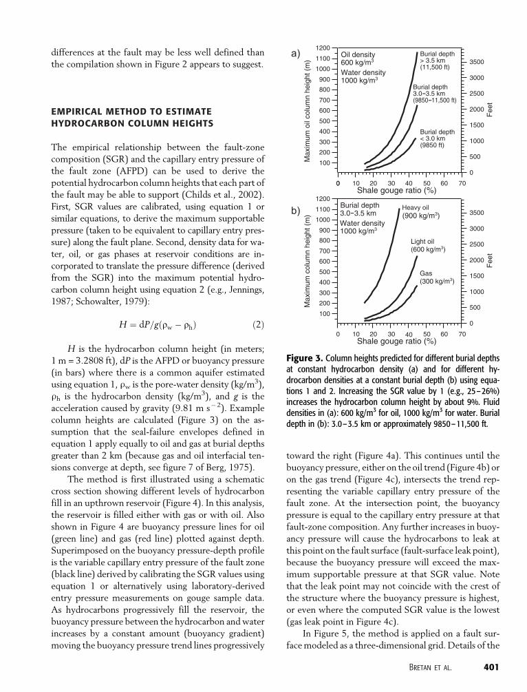
The method is first illustrated using a schematic

cross section showing different levels of hydrocarbon

fill in an upthrown reservoir (Figure 4). In this analysis,

the reservoir is filled either with gas or with oil. Also

shown in Figure 4 are buoyancy pressure lines for oil

(green line) and gas (red line) plotted against depth.

Superimposed on the buoyancy pressure-depth profile

is the variable capillary entry pressure of the fault zone

(black line) derived by calibrating the SGR values using

equation 1 or alternatively using laboratory-derived

entry pressure measurements on gouge sample data.

As hydrocarbons progressively fill the reservoir, the

buoyancy pressure between the hydrocarbon and water

increases by a constant amount (buoyancy gradient)

moving the buoyancy pressure trend lines progressively

toward the right (Figure 4a). This continues until the

buoyancy pressure, either on the oil trend (Figure 4b) or

on the gas trend (Figure 4c), intersects the trend rep-

resenting the variable capillary entry pressure of the

fault zone. At the intersection point, the buoyancy

pressure is equal to the capillary entry pressure at that

fault-zone composition. Any further increases in buoy-

ancy pressure will cause the hydrocarbons to leak at

this point on the fault surface (fault-surface leak point),

because the buoyancy pressure will exceed the max-

imum supportable pressure at that SGR value. Note

that the leak point may not coincide with the crest of

the structure where the buoyancy pressure is highest,

or even where the computed SGR value is the lowest

(gas leak point in Figure 4c).

In Figure 5, the method is applied on a fault sur-

face modeled as a three-dimensional grid. Details of the

Bretan et al. 401

Max

imum

oil

colu

mn

heig

ht (

m)

Oil density Burial depth> 3.5 km(11,500 ft)

Burial depth

Heavy oil

Shale gouge ratio (%)

Shale gouge ratio (%)

< 3.0 km(9850 ft)

Burial depth

1200

3500

3000

2500

2000

1500

1000

500

0

Fee

t

3500

3000

2500

2000

1500

1000

500

0

Fee

t

1100

1000

900

800

700

600

500

400

300

200

100

1200

0 100 20 30 40 50 60 70

100 20 30 40 50 60 70

1100

1000

900

800

700

600

500

400

300

200

100

3.0 3.5 km(9850 11,500 ft)

600 kg/m3

Water density1000 kg/m3

Burial depth

Water density1000 kg/m3

(900 kg/m3)

(600 kg/m3)Light oil

(300 kg/m3)Gas

Max

imum

col

umn

heig

ht (

m) 3.5 km3.0

Figure 3. Column heights predicted for different burial depthsat constant hydrocarbon density (a) and for different hy-drocarbon densities at a constant burial depth (b) using equa-tions 1 and 2. Increasing the SGR value by 1 (e.g., 25–26%)increases the hydrocarbon column height by about 9%. Fluiddensities in (a): 600 kg/m3 for oil, 1000 kg/m3 for water. Burialdepth in (b): 3.0–3.5 km or approximately 9850–11,500 ft.

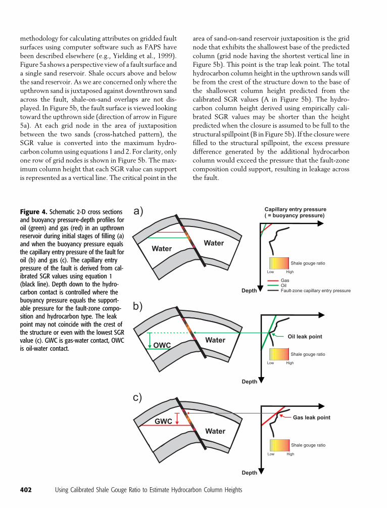
methodology for calculating attributes on gridded fault

surfaces using computer software such as FAPS have

been described elsewhere (e.g., Yielding et al., 1999).

Figure 5a shows a perspective view of a fault surface and

a single sand reservoir. Shale occurs above and below

the sand reservoir. As we are concerned only where the

upthrown sand is juxtaposed against downthrown sand

across the fault, shale-on-sand overlaps are not dis-

played. In Figure 5b, the fault surface is viewed looking

toward the upthrown side (direction of arrow in Figure

5a). At each grid node in the area of juxtaposition

between the two sands (cross-hatched pattern), the

SGR value is converted into the maximum hydro-

carbon column using equations 1 and 2. For clarity, only

one row of grid nodes is shown in Figure 5b. The max-

imum column height that each SGR value can support

is represented as a vertical line. The critical point in the

area of sand-on-sand reservoir juxtaposition is the grid

node that exhibits the shallowest base of the predicted

column (grid node having the shortest vertical line in

Figure 5b). This point is the trap leak point. The total

hydrocarbon column height in the upthrown sands will

be from the crest of the structure down to the base of

the shallowest column height predicted from the

calibrated SGR values (A in Figure 5b). The hydro-

carbon column height derived using empirically cali-

brated SGR values may be shorter than the height

predicted when the closure is assumed to be full to the

structural spillpoint (B in Figure 5b). If the closure were

filled to the structural spillpoint, the excess pressure

difference generated by the additional hydrocarbon

column would exceed the pressure that the fault-zone

composition could support, resulting in leakage across

the fault.

402 Using Calibrated Shale Gouge Ratio to Estimate Hydrocarbon Column Heights

Figure 4. Schematic 2-D cross sectionsand buoyancy pressure-depth profiles foroil (green) and gas (red) in an upthrownreservoir during initial stages of filling (a)and when the buoyancy pressure equalsthe capillary entry pressure of the fault foroil (b) and gas (c). The capillary entrypressure of the fault is derived from cal-ibrated SGR values using equation 1(black line). Depth down to the hydro-carbon contact is controlled where thebuoyancy pressure equals the support-able pressure for the fault-zone compo-sition and hydrocarbon type. The leakpoint may not coincide with the crest ofthe structure or even with the lowest SGRvalue (c). GWC is gas-water contact, OWCis oil-water contact.

CALIBRATION OF SHALE GOUGE RATIO BYBUOYANCY PRESSURE

The seal-failure envelope shown in Figure 2 was ob-

tained by plotting SGR against AFPD on one diagram.

Although this type of diagram does permit a general

trend of increasing SGR value supporting increasing

AFPD to be defined, the calibration implies that very

large hydrocarbon columns could be supported by very

high SGR values. We believe this to be unrealistic be-

cause the details of the generalized seal-failure envel-

ope in Figure 2 are likely to be masked by other factors

in the data.

We have reanalyzed, where possible, the calibra-

tion data according to buoyancy pressure and burial

depth of the faults. Three basic fluid type juxtapositions

can occur across faults, namely, hydrocarbons (oil or

gas) against water, hydrocarbons against other hydro-

carbons (oil-oil, gas-gas, oil-gas), and water juxtaposed

against water. Determining the values of buoyancy pres-

sure from these basic juxtaposition types can be further

complicated depending upon whether there is a

common or different aquifer across the fault, or wheth-

er the density of the hydrocarbons varies.

Hydrocarbons Against Water

The first general type of fluid juxtaposition is hydro-

carbons juxtaposed against water. Data used for the oil

against water (OW) and gas against water (GW)

calibration diagram should preferably satisfy two

criteria. First, pressure data are derived from two

preproduction wells situated close to the fault, having

one well located in the upthrown side and the other

well on the downthrown side. Second, the aquifer is at

the same pressure at the same depth on both sides of

the fault (common aquifer). In such cases, the pressure

in the hydrocarbon phase is higher than the pressure in

the water phase at the same depth on the fault. This

ensures that the AFPD are related to the hydrocarbon

capillary entry pressure of the fault zone. Where dif-

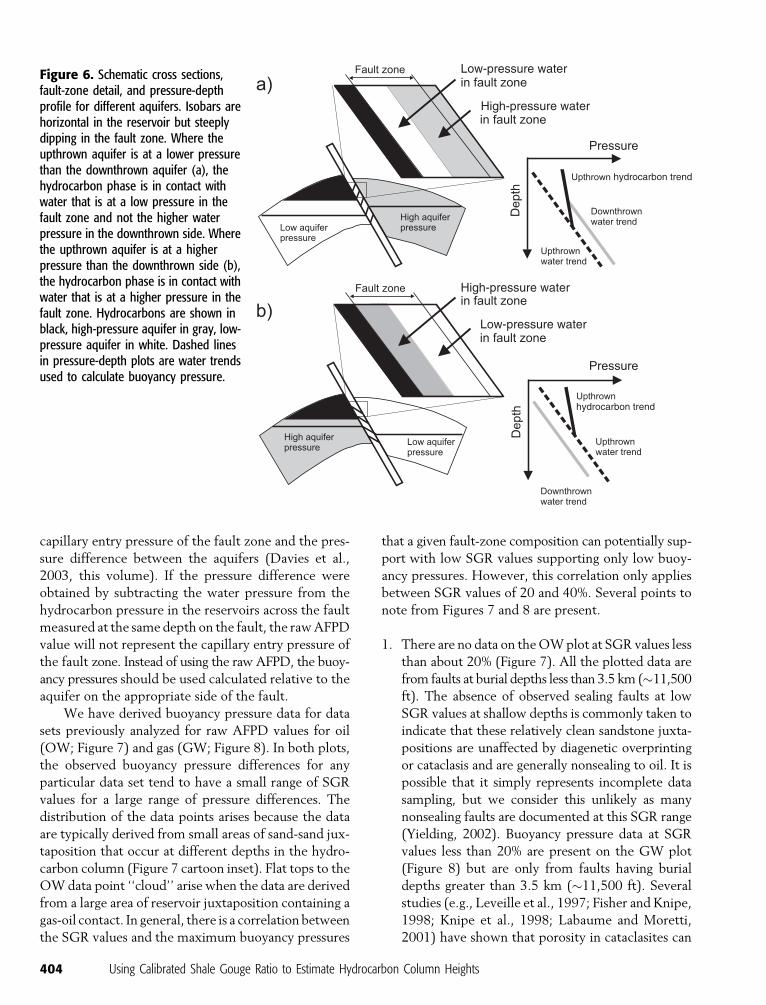
ferent aquifers are juxtaposed across a fault, pressure

isobars are horizontal in the reservoir but are likely to

be steeply inclined in the fault zone toward the lower

pressure aquifer (Davies et al., this volume). Each out-

er edge of the fault zone presents a different aquifer

pressure to any adjacent hydrocarbon column (Figure

6). Where there is a change in aquifer pressure across

the fault, the raw AFPD values are a combination of the

Bretan et al. 403

Figure 5. Schematic representation of asingle sand-on-sand juxtaposition along amodeled fault surface viewed in three di-mensions (a) and in a view looking directlytoward the upthrown side (b). Oil-bearingsands in the upthrown side shown in gray filland the water-bearing downthrown sands inoutline. The SGR value at every grid node isconverted into maximum column height,shown as a vertical line, using equations 1and 2. Computed maximum column for onlyone row of grid nodes is shown. The leakpoint is the grid node having the shortestcolumn. The maximum column height in theupthrown sand reservoir will be from thecrest of the structure down to the base of theshallowest column predicted from the SGRvalue (arrow A) and may be smaller than thecolumn height predicted using traditional fill-to-spill methods (arrow B).

capillary entry pressure of the fault zone and the pres-

sure difference between the aquifers (Davies et al.,

2003, this volume). If the pressure difference were

obtained by subtracting the water pressure from the

hydrocarbon pressure in the reservoirs across the fault

measured at the same depth on the fault, the raw AFPD

value will not represent the capillary entry pressure of

the fault zone. Instead of using the raw AFPD, the buoy-

ancy pressures should be used calculated relative to the

aquifer on the appropriate side of the fault.

We have derived buoyancy pressure data for data

sets previously analyzed for raw AFPD values for oil

(OW; Figure 7) and gas (GW; Figure 8). In both plots,

the observed buoyancy pressure differences for any

particular data set tend to have a small range of SGR

values for a large range of pressure differences. The

distribution of the data points arises because the data

are typically derived from small areas of sand-sand jux-

taposition that occur at different depths in the hydro-

carbon column (Figure 7 cartoon inset). Flat tops to the

OW data point ‘‘cloud’’ arise when the data are derived

from a large area of reservoir juxtaposition containing a

gas-oil contact. In general, there is a correlation between

the SGR values and the maximum buoyancy pressures

that a given fault-zone composition can potentially sup-

port with low SGR values supporting only low buoy-

ancy pressures. However, this correlation only applies

between SGR values of 20 and 40%. Several points to

note from Figures 7 and 8 are present.

1. There are no data on the OW plot at SGR values less

than about 20% (Figure 7). All the plotted data are

from faults at burial depths less than 3.5 km (�11,500

ft). The absence of observed sealing faults at low

SGR values at shallow depths is commonly taken to

indicate that these relatively clean sandstone juxta-

positions are unaffected by diagenetic overprinting

or cataclasis and are generally nonsealing to oil. It is

possible that it simply represents incomplete data

sampling, but we consider this unlikely as many

nonsealing faults are documented at this SGR range

(Yielding, 2002). Buoyancy pressure data at SGR

values less than 20% are present on the GW plot

(Figure 8) but are only from faults having burial

depths greater than 3.5 km (�11,500 ft). Several

studies (e.g., Leveille et al., 1997; Fisher and Knipe,

1998; Knipe et al., 1998; Labaume and Moretti,

2001) have shown that porosity in cataclasites can

404 Using Calibrated Shale Gouge Ratio to Estimate Hydrocarbon Column Heights

Figure 6. Schematic cross sections,fault-zone detail, and pressure-depthprofile for different aquifers. Isobars arehorizontal in the reservoir but steeplydipping in the fault zone. Where theupthrown aquifer is at a lower pressurethan the downthrown aquifer (a), thehydrocarbon phase is in contact withwater that is at a low pressure in thefault zone and not the higher waterpressure in the downthrown side. Wherethe upthrown aquifer is at a higherpressure than the downthrown side (b),the hydrocarbon phase is in contact withwater that is at a higher pressure in thefault zone. Hydrocarbons are shown inblack, high-pressure aquifer in gray, low-pressure aquifer in white. Dashed linesin pressure-depth plots are water trendsused to calculate buoyancy pressure.

be destroyed by solution and reprecipitation of

quartz at temperatures exceeding 90jC [equivalent

to burial depths of 3.0 km (�9850 ft) at normal

geothermal gradients]. The diagenetic overprint re-

duces the remaining low porosity in cataclastic fault

rocks resulting in an increased seal potential. Where

diagenetic overprinting is absent, cataclastic rocks

tend to have relatively uniform, or gradually de-

creasing, permeability when the phyllosilicate con-

tent ranges from 0 to 14% (Fisher and Knipe, 2001).

2. A difference in data point distribution at SGR val-

ues above about 40% is present. On the OW plot

(Figure 7), the buoyancy pressures do not increase

above about 3 bar or 43.5 psi between SGR values of

40 and 70%. The data on the GW plot (Figure 8)

exhibit a similar ‘‘plateau’’ distribution of data

points but at higher buoyancy pressures (�12 bar or

175 psi). A combination of three factors may cause

the lack of high (> 12 bar) buoyancy pressures at

SGR values above 40%. First, the absence of data

may simply reflect incomplete data sampling. Our

current fault database does not contain any reliably

mapped faults that juxtapose hydrocarbon-bearing

sands against water-bearing sands having minimum

SGR values greater than 40% and well-constrained

buoyancy pressures greater than 3 bar for oil or 12

bar for gas. Second, all the data points may originate

from sand-on-sand juxtapositions that occur lower

in the hydrocarbon column and therefore are not at

seal capacity, or from traps that are controlled by dip

closure away from the fault and not by fault seal. A

third reason for the plateau distribution of data lies

in the observation that fault-zone hydraulic pro-

cesses appear not to change when the SGR value

exceeds about 45–50%. A seal having an SGR value

of 90% will not be significantly stronger, and there-

fore will not support a significantly greater hydro-

carbon column, than a seal having an SGR value of

Bretan et al. 405

Shale gouge ratio (%)

Buo

yanc

y pr

essu

re (

bar)

100

10

1

0.1

0 10 20 30 40 50 60 70

10

100

1000(psi)

Figure 7. Shale gouge ratio againstbuoyancy pressure calibration for oil-bearing sands juxtaposed against water.All data on the calibration plot are de-rived from faults at burial depths lessthan 3.5 km. Data color coded by depth:less than 3.0 km (�9850 ft) dark blue;3.0–3.5 km (�9850–11,500 ft) red.

40%. Microstructural (Fisher and Knipe, 1998,

2001) and oil field studies (Ottesen Ellevset et al.,

1998) indicate that phyllosilicate smear rocks having

an SGR range between 40 and 100% are likely to

have uniform permeability (< 0.001 md). Similarly,

Fulljames et al. (1997) show that the probability for

seal is independent of CSP above a certain CSP

value, although the actual value is not documented

(figure 5 of Fulljames et al., 1997).

The main point to emerge from the calibration

plots based on buoyancy pressure is that a global seal-

failure envelope based on AFPD has overgeneralized

the relationship between increasing SGR values and

increasing pressure that the fault seal can support. For

gas-bearing traps (Figure 8), depth of burial, especially

for fault rocks at the low end of the SGR spectrum

(clay-poor cataclastic fault rocks) strongly influences

the seal-failure envelope. Although SGR values as low

as 10% appear capable of supporting gas columns, seal-

ing is most likely to be the result of pore-throat re-

duction by diagenetic occlusion instead of the presence

of phyllosilicates in the fault zone. For oil-bearing traps,

the effect of depth of burial cannot be fully evaluated

because all data were derived from faults at burial

depths less then 3.5 km (�11,500 ft) (oil is destroyed

at significantly greater depths). More data are still re-

quired to fully define seal-failure envelopes for the sep-

arate gas and oil calibration plots.

Hydrocarbons Against Hydrocarbons

The second general type of fluid juxtaposition is where

gas or oil-bearing intervals are juxtaposed against other

gas- or oil-bearing intervals having the same fluid den-

sity. These data provide an insight into the fluid content

406 Using Calibrated Shale Gouge Ratio to Estimate Hydrocarbon Column Heights

Figure 8. Shale gouge ratio againstbuoyancy pressure calibration for gas-bearing sands juxtaposed against water.Data color-coded by depth: less than3.0 km (�9850 ft) dark blue; 3.0–3.5 km(�9850–11,500 ft) red; 3.5–5.5 km(�11,500–18,050 ft) green.

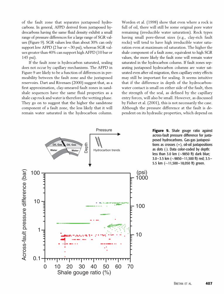
of the fault zone that separates juxtaposed hydro-

carbons. In general, AFPD derived from juxtaposed hy-

drocarbons having the same fluid density exhibit a small

range of pressure differences for a large range of SGR val-

ues (Figure 9). SGR values less than about 30% can only

support low AFPD (2 bar or �30 psi), whereas SGR val-

ues greater than 40% can support high AFPD (10 bar or

145 psi).

If the fault zone is hydrocarbon saturated, sealing

does not occur by capillary mechanisms. The AFPD in

Figure 9 are likely to be a function of differences in per-

meability between the fault zone and the juxtaposed

reservoirs. Dart and Rivenaes (2000) suggest that, as a

first approximation, clay-smeared fault zones in sand-

shale sequences have the same fluid properties as a

shale cap rock and water is therefore the wetting phase.

They go on to suggest that the higher the sandstone

component of a fault zone, the less likely that it will

remain water saturated in the hydrocarbon column.

Worden et al. (1998) show that even where a rock is

full of oil, there will still be some original pore water

remaining (irreducible water saturation). Rock types

having small pore-throat sizes (e.g., clay-rich fault

rocks) will tend to have high irreducible water satu-

ration even at maximum oil saturation. The higher the

shale component of a fault zone, equivalent to high SGR

values, the more likely the fault zone will remain water

saturated in the hydrocarbon column. If fault zones sep-

arating juxtaposed hydrocarbon columns are water sat-

urated even after oil migration, then capillary entry effects

may still be important for sealing. It seems intuitive

that if the difference in depth of the hydrocarbon-

water contact is small on either side of the fault, then

the strength of the seal, as defined by the capillary

entry forces, will also be small. However, as discussed

by Fisher et al. (2001), this is not necessarily the case.

Although the pressure difference at the fault is de-

pendent on its hydraulic properties, which depend on

Bretan et al. 407

Figure 9. Shale gouge ratio againstacross-fault pressure difference for juxta-posed hydrocarbons. Gas-gas juxtaposi-tions as crosses (+), oil-oil juxtapositionsas dots (�). Data color-coded by depth:less than 3.0 km (�9850 ft) dark blue;3.0–3.5 km (�9850–11,500 ft) red; 3.5–5.5 km (�11,500–18,050 ft) green.

fault-zone composition as reflected by SGR, the de-

tails of the SGR-AFPD relationship for juxtaposed

hydrocarbons depend upon the aquifer pressure and

the filling/migration history of the reservoirs adjacent

to the fault.

Water Against Water

The final general type of fluid juxtaposition is water

juxtaposed against water across a fault (Figure 10). The

AFPD do not reflect the capillary entry effects of a

membrane seal (Watts, 1987; Yielding et al., 1997).

However, there is a general relationship between SGR

values and AFPD derived from water-on-water juxta-

position. High SGR values support high AFPD values.

Very low fault-zone permeability at high SGR values

most probably causes the differences in pressure that

would retard the flow rate of water across the fault.

Heum (1996) refers to seals of this type as hydraulic

resistance seals. A similar SGR-AFPD correlation is

observed for Brent production data but having much

larger pressure differences at a given SGR (Harris et al.,

2002).

UNCERTAINTIES

Prediction of hydrocarbon column heights is not an

exact science. The method described in the previous

section relies on the availability of pressure data and the

empirical relationship between fault-zone rock type

(estimated using the SGR algorithm) and supportable

across-fault pressures (assumed to represent the capil-

lary entry pressure for hydrocarbons). Further uncer-

tainties arise from the estimate for the V shale parameter

and the geometric construction of the structural model.

All these uncertainties should be taken into account

when estimating column heights.

408 Using Calibrated Shale Gouge Ratio to Estimate Hydrocarbon Column Heights

Figure 10. Shale gouge ratio againstacross-fault pressure difference for jux-taposed aquifers. The data exhibit a smallrange of pressure differences for a largerange of SGR values. Data color coded bydepth: less than 3.0 km (�9850 ft) darkblue; 3.0–3.5 km (�9850–11,500 ft)red; 3.5–5.5 km (�11,500–18,050 ft)green.

Pressure Data

The lack of pressure data, especially in frontier explo-

ration areas, commonly prevents the detailed calibra-

tion of SGR values. The most ideal case is where the

SGR values are locally calibrated on the structure using

preproduction pressure data from wells located on either

side of the fault. This ensures that the predicted rela-

tionship incorporates locally derived parameters. Failing

this, the SGR values could be calibrated using pressure

data from wells in nearby parts of the same basin. In

cases where no pressure data exist, the SGR values

can be compared to calibration plots based on buoy-

ancy pressure. However, care should be taken to use

data points on these plots that were derived using a

similar methodology for calculating SGR and were ob-

tained from faults that have a similar geohistory to the

fault of interest.

Even if reliable pressure data are available, an SGR-

buoyancy pressure calibration may not derive the entry

pressure of the fault zone. Figure 11 shows a schematic

cross section and SGR-buoyancy pressure calibration

derived from a fault in the central North Sea. The upper

part of the fault is leaking because gas on either side of

the fault lies on the same pressure trend (pressure equal-

ization across the fault). The lower part is sealing, as

there is a difference in observed pressure between the

high-pressure aquifer in the downthrown side and

the lower pressure gas in the upthrown side. Below the

gas-water juxtaposition, the fault separates differently

pressured aquifers. A plot of SGR against calculated

buoyancy pressure produces a distribution of points

that is totally different to the calibration plots shown in

Figures 2 and 8. There appears to be no increase in

buoyancy pressure for increasing SGR for the area of

the fault that is separating gas from water (green in

Bretan et al. 409

Figure 11. Cartoon cross section,depth-pressure plot and calibration plotderived from a fault in the central NorthSea. Buoyancy pressure calculated usingthe water trend in the upthrown sideof the fault for the juxtaposition of low-pressure gas and high-pressure water(green) and the gas against gas juxtapo-sition (black). No apparent value for theonset of fault seal is present.

Figure 11). The part of the fault that is leaking to gas

shows a slight increase in SGR for increasing buoyancy

pressure (black in Figure 11). Initial gas leakage

presumably occurred at a lower buoyancy pressure

corresponding to the fault entry pressure, but continued

gas charge and fill has produced longer gas columns and

higher buoyancy pressure that now exceed the entry

pressure. This example shows that, for some data sets,

the present-day pressure data cannot be used to re-

construct seal failure and hence predict column height

(see also Fisher et al., 2001).

Vshale

Several workers have discussed uncertainties in pre-

dicting fault-zone properties, especially the proportion

of fine-grained material in the fault (e.g., Childs et al.,

1997; Hesthammer and Fossen, 2000). Of key concern

is the methodology used to estimate V shale. Different

vintages of V shale analysis of the same well by different

petrophysicists working in the same company can be

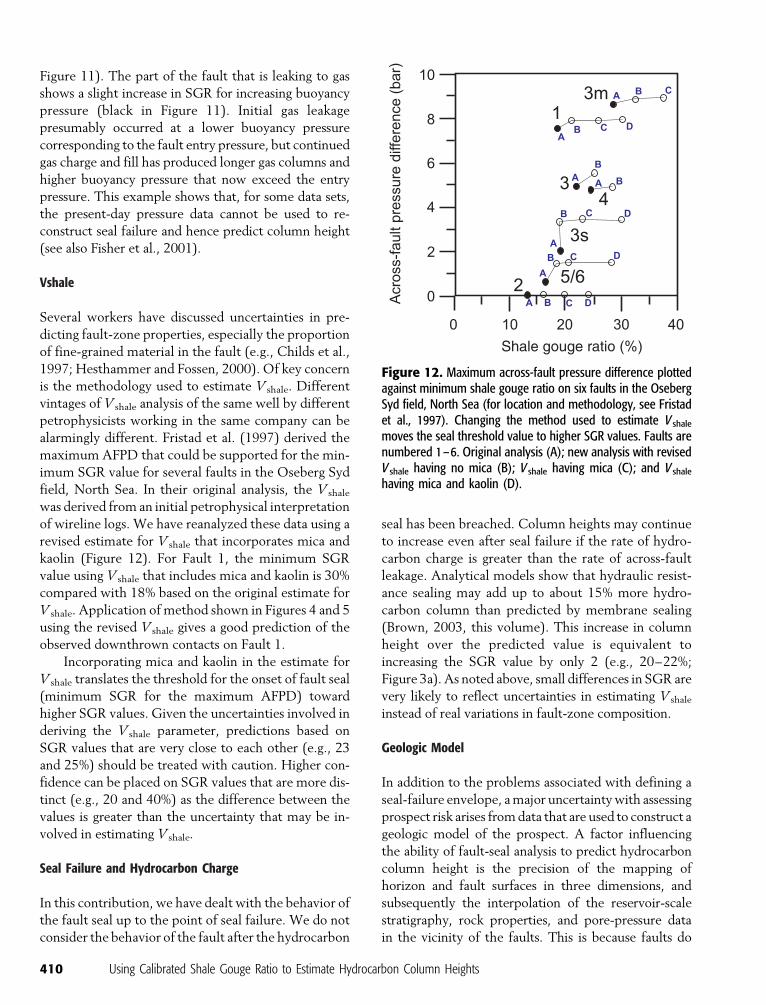
alarmingly different. Fristad et al. (1997) derived the

maximum AFPD that could be supported for the min-

imum SGR value for several faults in the Oseberg Syd

field, North Sea. In their original analysis, the V shale

was derived from an initial petrophysical interpretation

of wireline logs. We have reanalyzed these data using a

revised estimate for V shale that incorporates mica and

kaolin (Figure 12). For Fault 1, the minimum SGR

value using V shale that includes mica and kaolin is 30%

compared with 18% based on the original estimate for

V shale. Application of method shown in Figures 4 and 5

using the revised V shale gives a good prediction of the

observed downthrown contacts on Fault 1.

Incorporating mica and kaolin in the estimate for

V shale translates the threshold for the onset of fault seal

(minimum SGR for the maximum AFPD) toward

higher SGR values. Given the uncertainties involved in

deriving the V shale parameter, predictions based on

SGR values that are very close to each other (e.g., 23

and 25%) should be treated with caution. Higher con-

fidence can be placed on SGR values that are more dis-

tinct (e.g., 20 and 40%) as the difference between the

values is greater than the uncertainty that may be in-

volved in estimating V shale.

Seal Failure and Hydrocarbon Charge

In this contribution, we have dealt with the behavior of

the fault seal up to the point of seal failure. We do not

consider the behavior of the fault after the hydrocarbon

seal has been breached. Column heights may continue

to increase even after seal failure if the rate of hydro-

carbon charge is greater than the rate of across-fault

leakage. Analytical models show that hydraulic resist-

ance sealing may add up to about 15% more hydro-

carbon column than predicted by membrane sealing

(Brown, 2003, this volume). This increase in column

height over the predicted value is equivalent to

increasing the SGR value by only 2 (e.g., 20–22%;

Figure 3a). As noted above, small differences in SGR are

very likely to reflect uncertainties in estimating V shale

instead of real variations in fault-zone composition.

Geologic Model

In addition to the problems associated with defining a

seal-failure envelope, a major uncertainty with assessing

prospect risk arises from data that are used to construct a

geologic model of the prospect. A factor influencing

the ability of fault-seal analysis to predict hydrocarbon

column height is the precision of the mapping of

horizon and fault surfaces in three dimensions, and

subsequently the interpolation of the reservoir-scale

stratigraphy, rock properties, and pore-pressure data

in the vicinity of the faults. This is because faults do

410 Using Calibrated Shale Gouge Ratio to Estimate Hydrocarbon Column Heights

Figure 12. Maximum across-fault pressure difference plottedagainst minimum shale gouge ratio on six faults in the OsebergSyd field, North Sea (for location and methodology, see Fristadet al., 1997). Changing the method used to estimate V shale

moves the seal threshold value to higher SGR values. Faults arenumbered 1–6. Original analysis (A); new analysis with revisedV shale having no mica (B); V shale having mica (C); and V shale

having mica and kaolin (D).

not have homogeneous capillary entry properties along

their length. Different rock types will make a different

contribution to the fault-zone composition, depending

upon throw and lateral variation in the V shale compo-

nent, at different parts of the fault. Furthermore, the

depths of the reservoir intervals and their juxtapositions

across the fault, relative to pressure gradients, will vary

depending upon fault throw. Intervals that initially occur

in a water leg may pass along strike into an oil or gas leg.

Geologic History

Many workers have discussed burial depth at the time

of faulting and the subsequent burial history on seal

development (e.g., Knipe, 1992; Fisher and Knipe,

1998). In general, increasing the burial depth is likely to

enhance the seal potential especially for clay-poor fault

zones. However, seal integrity may be compromised if

the faults are optimally oriented for renewed slip in the

present-day tectonic stress field (Castillo, 2000). El-

evated pore pressures caused by hydrocarbons may re-

sult in hydraulic fracturing or fluid flow along faults

(Finkbeiner et al., 2001).

Faults in the database used to derive the ‘‘seal-

failure envelope’’ in Figure 2 are normal faults having

dip-slip movement. As far as the authors are aware,

there are no published calibration data for dip-slip re-

verse, oblique-slip, or strike-slip faults. The paucity of

data for oblique-slip faults may lie in the inherent

difficulty in recognizing oblique-slip motion on faults

imaged on seismic data. Note that SGR values can be

derived from faults having oblique-slip movement but

only where there is no lateral variation in the stra-

tigraphy, such as channels, that occur along the strike of

the fault. This is because the SGR value is a ratio where

the critical factor is the slip across the stratigraphy.

CONCLUSIONS

� In an exploration context, SGR values can be em-

pirically calibrated with pressure data to define

depth-dependent seal-failure envelopes. The seal-

failure envelope provides a method to estimate the

maximum height of a hydrocarbon column.� Column heights estimated using calibrated SGR val-

ues may be smaller than columns estimated using

‘‘fill-to-structural spill’’ methods. Across-fault leak-

age of hydrocarbons is not confined to the crest of

the structure or even to areas where the computed

SGR value is lowest. The point on a fault where hy-

drocarbons may leak depends upon the buoyancy

pressure (pressure difference between the hydro-

carbon and water phases) and the three-dimensional

distribution of the variable capillary entry pressure of

the fault zone, as derived from SGR values.� Established calibration diagrams based on AFPD have

overgeneralized the relationship between increasing

SGR values and increasing supportable pressures.� Calibration diagrams based on buoyancy pressure

show that gas and oil data exhibit a correlation be-

tween increasing SGR and increasing buoyancy pres-

sure but only between SGR values of 20 and 40%.

More data are still required to define individual seal-

failure envelopes for oil and gas.� The onset of seal for gas is dependent upon depth of

burial especially at SGR values less than 15%. For oil,

the onset for seal occurs at an SGR value of about 20%.� No increase in the strength of a seal occurs, as re-

flected by an increase in maximum supportable buoy-

ancy pressure, at SGR values greater than about 40%

both for gas and for oil data. Column heights do not

continue to increase over the SGR range 50–100%.� Estimating hydrocarbon column heights using fault-

seal attribute data ultimately depends upon the geo-

logic input into the model, in particular the pressure

data, volumetric shale fraction (V shale), of the in-

tervals and the precision of the three-dimensional

mapping and interpolation of reservoir geometry

and zonal properties in the vicinity of the fault.

REFERENCES CITED

Berg, R. R., 1975, Capillary pressure in stratigraphic traps: AAPGBulletin, v. 59, p. 939–956.

Bjorkum, P. A., O. Walderhaug, and P. H. Nadeau, 1998, Physicalconstraints on hydrocarbon leakage and trapping revisited:Petroleum Geoscience, v. 4, p. 237–239.

Bouvier, J. D., C. H. Kaars-Sijpesteijn, D. F. Kluesner, C. C.Onyejekwe, and R. C. Van Der Pal, 1989, Three-dimensionalseismic interpretation and fault sealing investigations, NunRiver field, Nigeria: AAPG Bulletin, v. 73, p. 1397–1414.

Brown, A., 2003, Capillary pressure effects on fault sealing, AAPGBulletin v. 87, p. 381–395.

Castillo, D., 2000, Fault seal integrity in ZOC ‘‘A’’: Can it bequantified and is it predictable?: PESA News, February/March2000, p. 56–60.

Childs, C., J. Watterson, and J. J. Walsh, 1997, Complexity in faultzone structure and implications for fault seal prediction, in P.Møller-Pedersen and A. G. Koestler, eds., Hydrocarbon seals:Importance for exploration and production: NorwegianPetroleum Society (NPF) Special Publication 7, Singapore,Elsevier, p. 61–72.

Childs, C., O. Sylta, S. Moriya, J. J. Walsh, and T. Manzocchi,2002, A method for including the capillary properties of faultsin hydrocarbon migration models, in A. G. Koestler and

Bretan et al. 411

R. Hunsdale, eds., Hydrocarbon seal quantification: Amster-dam, Elsevier, Norwegian Petroleum Society (NPF) SpecialPublication 11, p. 127–139.

Dart, C., and J. C. Rivenaes, 2000, Evaluation of reservoir faultcompartmentalisation— Do we have the tools we need?, inHydrocarbon seal quantification: Norwegian Petroleum So-ciety Conference Extended Abstracts, Stavanger, October2000, p. 121–124.

Davies, R., L. An, A. Mathis, P. Jones, and C. Cornette, 2003, Faultseal analysis SMI36 Field, Gulf of Mexico: AAPG Bulletin,v. 87, p. 479–491.

Finkbeiner, T., M. Zoback, P. Flemings, and B. Stump, 2001, Stress,pore pressure, and dynamically constrained hydrocarboncolumns in the South Eugene Island 330 field, northern Gulfof Mexico: AAPG Bulletin, v. 85, p. 1007–1031.

Firoozabadi, A., and H. J. Ramey, 1988, Surface tension of water-hydrocarbon systems at reservoir conditions: Journal ofCanadian Petroleum Technology, v. 27, p. 41–48.

Fisher, Q. J., and R. J. Knipe, 1998, Fault sealing processes insiliciclastic sediments, in G. Jones, Q. J. Fisher, and R. J.Knipe, eds., Faulting, fault sealing and fluid flow in hydro-carbon reservoirs: Geological Society (London) Special Pub-lication 147, p. 117–134.

Fisher, Q. L., and R. J. Knipe, 2001, The permeability of faultswithin siliciclastic petroleum reservoirs of the North Sea andNorwegian Continental Shelf: Marine and Petroleum Geology,v. 18, p. 1063–1081.

Fisher, Q. J., S. D. Harris, E. McAllister, R. J. Knipe, and A. J.Bolton, 2001, Hydrocarbon flow across faults by capillaryleakage revisited: Marine and Petroleum Geology, v. 18,p. 251–257.

Freeman, B., G. Yielding, D. T. Needham, and M. E. Badley, 1998,Fault seal prediction: The gouge ratio method, in M. P.Coward, T. S. Daltaban, and H. Johnson, eds., Structuralgeology in reservoir characterization: Geological Society(London) Special Publication 127, p. 19–25.

Fristad, T., A. Groth, G. Yielding, and B. Freeman, 1997,Quantitative fault seal prediction: A case study from OsebergSyd, in P. Møller-Pedersen and A. G. Koestler, eds., Hydro-carbon seals: Importance for exploration and production:Singapore, Elsevier, Norwegian Petroleum Society (NPF)Special Publication 7, p. 107–124.

Fulljames, J. R., L. J. J. Zijerveld, and R. C. M. W. Franssen,1997, Fault seal processes: systematic analyses of fault sealsover geological and production time scales, in P. Møller-Pedersen and A. G. Koestler, eds., Hydrocarbon seals:Importance for exploration and production: Singapore, Else-vier, Norwegian Petroleum Society (NPF) Special Publication7, p. 51–59.

Gibson, R. G., 1994, Fault-zone seals in siliciclastic strata of theColumbus Basin, offshore Trinidad: AAPG Bulletin, v. 78,p. 1372–1385.

Gibson, R. G., 1998, Physical character and fluid-flow properties ofsandstone-derived fault gouge, in M. P. Coward, T. S.Daltaban, and H. Johnson, eds., Structural geology in reservoircharacterization: Geological Society (London) Special Pub-lication 127, p. 83–97.

Grauls, D., F. Pascaud, and T. Rives, 2002, Quantitative fault sealassessment in hydrocarbon-compartmentalised structuresusing fluid pressure data, in A. G. Koestler and R. Hunsdale,Hydrocarbon seal quantification: Amsterdam, Elsevier, Nor-wegian Petroleum Society (NPF) Special Publication 11,p. 141–156.

Harris, D., G. Yielding, P. Levine, G. Maxwell, P. T. Rose, andP. A. R. Nell, 2002, Using shale gouge ratio (SGR) to modelfaults as transmissibility barriers in reservoirs: An example

from the Strathspey field, North Sea: Petroleum Geoscience,v. 8, p. 167–176.

Hesthammer, J., and H. Fossen, 2000, Uncertainties associated withfault sealing analysis: Petroleum Geoscience, v. 6, p. 37–45.

Heum, O. R., 1996, A fluid dynamic classification of hydrocarbonentrapment: Petroleum Geoscience, v. 2, p. 145–158.

Ingram, G. M., J. L. Urai, and M. A. Naylor, 1997, Sealing processesand top seal assessment, in P. Møller-Pedersen and A. G.Koestler, eds., Hydrocarbon seals: Importance for explorationand production: Singapore, Elsevier, Norwegian PetroleumSociety (NPF) Special Publication 7, p. 165–174.

Jennings, J. B., 1987, Capillary pressure techniques: Application toexploration and development geology: AAPG Bulletin, v. 71,p. 1196–1209.

Jev, B. I., C. H. Kaars-Sijpesteijn, M. P. A. M. Peters, N. L. Watts,and J. T. Wilkie, 1993, Akaso Field, Nigeria: Use of integrated3-D seismic, fault slicing, clay smearing, and RFT pressure dataon fault trapping and dynamic leakage: AAPG Bulletin, v. 77,p. 1389–1404.

Knipe, R. J., 1992, Faulting processes and fault seal, in R. M. Larsen,H. Brekke, B. T. Larsen, and E. Talleraas, eds., Structural andtectonic modelling and its application to petroleum geology:Stavanger, Elsevier, Norwegian Petroleum Society (NPF)Special Publication 1, p. 325–342.

Knipe, R. J., 1997, Juxtaposition and seal diagrams to help analyzefault seals in hydrocarbon reservoirs: AAPG Bulletin, v. 81,p. 187–195.

Knipe, R. J., G. Jones, and Q. J. Fisher, 1998, Faulting, fault sealingand fluid flow in hydrocarbon reservoirs: An introduction, inG. Jones, Q. J. Fisher, and R. J. Knipe, eds., Faulting, faultsealing and fluid flow in hydrocarbon reservoirs: GeologicalSociety (London) Special Publication 147, p. vii–xxi.

Labaume, P., and I. Moretti, 2001, Diagenesis-dependence ofcataclastic thrust fault zone sealing in sandstones. Examplefrom the Bolivian Sub-Andean Zone: Journal of StructuralGeology, v. 23, p. 1659–1675.

Leveille, G. P., R. Knipe, C. More, D. Ellis, G. Dudley, G. Jones,Q. J. Fisher, and G. Allinson, 1997, Compartmentalizationof Rotliegendes gas reservoirs by sealing faults, Jupiterfields area, southern North Sea, in K. Zeigler et al., eds.,Petroleum geology of the southern North Sea; future potential:Geological Society (London) Special Publication 123,p. 87–104.

Manzocchi, T., J. J. Walsh, P. A. R. Nell, and G. Yielding, 1999,Fault transmissibility multipliers for flow simulation models:Petroleum Geoscience, v. 5, p. 53–63.

Naruk, S. J., and J. W. Handschy, 1997, Characterization andprediction of fault seal parameters: empirical data (abs.):AAPG Hedberg Research Conference on ‘‘Reservoir scaledeformation: characterisation and prediction’’, Bryce, Utah.

O’Connor, S. J., 2000, Hydrocarbon-water interfacial tension valuesat reservoir conditions: Inconsistencies in the technicalliterature and the impact on maximum oil and gas columnheight calculations: AAPG Bulletin, v. 84, p. 1537–1541.

Ottesen Ellevset, S., R. J. Knipe, T. S. Olsen, Q. Fisher, and G.Jones, 1998, Fault controlled communication in the SleipnerVest Field, Norwegian Continental Shelf: Detailed, quantita-tive input for reservoir simulation and well planning, in G.Jones, Q. J. Fisher, and R. J. Knipe, eds., Faulting, fault sealingand fluid flow in hydrocarbon reservoirs: Geological Society(London) Special Publication 147, p. 283–297.

Rodgers, S., 1999, Discussion: ‘‘Physical constraints on hydrocarbonleakage and trapping revisited— further aspects’’: PetroleumGeoscience, v. 5, p. 421–423.

Schowalter, T. T., 1979, Mechanics of secondary hydrocarbonmigration and entrapment: AAPG Bulletin, v. 63, p. 723–760.

412 Using Calibrated Shale Gouge Ratio to Estimate Hydrocarbon Column Heights

Vavra, C. L., J. G. Kaldi, and R. M. Sneider, 1992, Geologicalapplications of capillary pressure: A review: AAPG Bulletin,v. 76, p. 840–850.

Watts, N., 1987, Theoretical aspects of cap-rock and fault seals forsingle- and two-phase hydrocarbon columns: Marine andPetroleum Geology, v. 4, p. 274–307.

Welbon, A. L., A. Beach, P. J. Brockbank, O. Fjeld, S. D. Knott,T. Pedersen, and S. Thomas, 1997, Fault seal analysis inhydrocarbon exploration and appraisal: Examples from off-shore mid-Norway, in P. Møller-Pedersen and A. G. Koestler,eds., Hydrocarbon seals: Importance for exploration andproduction: Singapore, Elsevier, Norwegian Petroleum Society(NPF) Special Publication 7, p. 165–174.

Worden, R. H., N. H. Oxtoby, and P. C. Smalley, 1998, Can oilemplacement prevent quartz cementation in sandstones?Petroleum Geoscience, v. 4, p. 129–137.

Yielding, G., 2002, Shale gouge ratio— Calibration by geohistory,in A. G. Koestler and R. Hunsdale, Hydrocarbon sealquantification: Amsterdam, Elsevier, Norwegian PetroleumSociety (NPF) Special Publication 11, p. 1–15.

Yielding, G., B. Freeman, and T. Needham, 1997, QuantitativeFault Seal Prediction: AAPG Bulletin, v. 81, p. 897–917.

Yielding, G., J. A. Overland, and G. Byberg, 1999, Characterizationof fault zones for reservoir modeling: An example from theGullfaks field, northern North Sea: AAPG Bulletin, v. 83,p. 925–951.

Bretan et al. 413