163
USING EARTH OBSERVATION SATELLITES TO EXPLORE FOREST DYNAMICS ACROSS LARGE AREAS Samuel Hislop

USING EARTH OBSERVATION SATELLITES TO
EXPLORE FOREST DYNAMICS ACROSS LARGE AREAS
Samuel Hislop


USING EARTH OBSERVATION SATELLITES TO EXPLORE
FOREST DYNAMICS ACROSS LARGE AREAS
DISSERTATION
to obtain the degree of doctor at the University of Twente,
on the authority of the rector magnificus, prof.dr. T.T.M. Palstra,
on account of the decision of the Doctorate Board, to be publicly defended
on Wednesday 18 September 2019 at 14:45 hrs
by
Samuel Raymond Hislop born on 30 September 1980
in Korumburra, Australia

This thesis has been approved by Prof.dr. S. Jones, supervisor Prof.dr. A. K. Skidmore, supervisor Dr. A. Haywood, co-supervisor Dr. M. Soto-Berelov, co-supervisor
ITC dissertation number 362 ITC, P.O. Box 217, 7500 AE Enschede, The Netherlands
ISBN 978-90-365-4836-6 DOI 10.3990/1.9789036548366
Cover designed by Samuel Hislop Printed by ITC Printing Department Copyright © 2019 by Samuel Hislop

Graduation committee:
Chairman/Secretary Dean of the Faculty University of Twente
Supervisors Prof.dr. S. Jones RMIT University Prof.dr. A. K. Skidmore University of Twente
Co-supervisor Dr. A. Haywood European Forest Institute
Members Prof.dr.ir. A. Veldkamp University of Twente Prof.dr. F. D. van der Meer University of Twente Prof.dr. L. Eklundh Lund University Dr.ir J. Verbesselt Wageningen University


Acknowledgements My sincerest appreciation to all who have contributed to this thesis and supported me throughout my PhD. Without your help, it would not have been possible. I am especially indebted to my four supervisors: Prof Simon Jones and Dr Mariela Soto-Berelov from RMIT, Prof Andrew Skidmore from ITC and Dr Andrew Haywood from the European Forest Institute. Simon, thank you for your unwavering support, encouragement and wisdom over the past three and a half years. Mariela, both your professional help and friendship have been invaluable. Andrew (Skidmore), thank you for accepting me into the double-badged program, making me feel at home in Enschede, and challenging my thinking. Andrew (Haywood), your unique mix of high-level strategic thinking and detailed technical knowledge has been of utmost benefit. I also thank Trung Nguyen for his technical assistance and support throughout our shared PhD journeys.
My thanks go also to Graeme Kernich and the team at FrontierSI (formally CRCSI), and Salahuddin Ahmad, Liam Costello and the team at the Department of Environment, Land, Water and Planning, who provided the necessary backdrop and funding for this research.
I would also like to thank my fellow PhDs and postdocs at both RMIT and ITC. At RMIT: Trung, Bryan, Sam, Daisy, Chats, Chithra, Ahmad, Jenna, Fiona, Luke, Mahyat and Chermelle. And at ITC: Jing, Yifang, Haidi, Marcelle, Linlin, Alby, Haili, Xin, Tawanda, Elnaz and Xi. To all of you, and other early career scientists who I crossed paths with over the last few years, your friendship and support has made my PhD experience so much more rewarding. At times, a PhD is a lonely endeavour, but being able to share the journey with like-minded people relieves the loneliness.
I also thank all the university staff who have assisted me in various matters, from both RMIT and ITC, especially the Science HDR team at RMIT and Loes Colenbrander and Esther López-Hondebrink at ITC. To Esther in particular, thank you for all your assistance and for translating the summary of this thesis into Dutch.

ii
To all my friends in various parts of the world, you mean more to me than you know. Sometimes you’ve provided a bed for the night, other times you’ve been a sounding board for ideas. But most of all, we’ve just passed time together. Finally, to my family, without whom I would not have reached this milestone. To my mother and father, especially, thank you for always being there for me over the years, and not questioning my non-linear career trajectory. To my sisters, Jennifer and Alison, and their families, thank you for reminding me that life is comprised of much more than can be seen from space.

iii
Table of Contents Acknowledgements ................................................................................................. i Table of Contents .................................................................................................. iii List of figures .......................................................................................................... v List of tables ......................................................................................................... viii Chapter 1: General Introduction .......................................................................... 1
1.1 Forest monitoring and reporting ................................................................ 2 1.2 Satellite Earth observation time series ...................................................... 4 1.3 This research ................................................................................................. 8
Chapter 2: Using Landsat spectral indices in time series to assess wildfire disturbance and recovery ..................................................................................... 11
2.1 Introduction ................................................................................................ 13 2.2 Materials and methods ............................................................................... 15 2.3 Results .......................................................................................................... 24 2.4 Discussion ................................................................................................... 30 2.5 Conclusions ................................................................................................. 34
Chapter 3: A fusion approach to forest disturbance mapping using time series ensemble techniques ............................................................................................ 35
3.1 Introduction ................................................................................................ 37 3.2 Materials and methods ............................................................................... 38 3.3 Results .......................................................................................................... 45 3.4 Discussion ................................................................................................... 50 3.5 Conclusions ................................................................................................. 54
Chapter 4: The relationship between spectral disturbance magnitude and recovery length ...................................................................................................... 55
4.1 Introduction ................................................................................................ 57 4.2 Materials and methods ............................................................................... 58 4.3 Results .......................................................................................................... 66 4.4 Discussion ................................................................................................... 74 4.5 Conclusions ................................................................................................. 77
Chapter 5: Wildfire disturbance and recovery in temperate and boreal forests worldwide .............................................................................................................. 79
5.1 Introduction ................................................................................................ 81 5.2 Materials and methods ............................................................................... 84 5.3 Results .......................................................................................................... 89

iv
5.4 Discussion ................................................................................................... 97 5.5 Conclusions ............................................................................................... 101
Chapter 6: Synthesis ........................................................................................... 103 6.1 Summary of results ................................................................................... 104 6.2 Broader implications of research ........................................................... 111 6.3 Future directions and opportunities ...................................................... 113 6.4 Final remarks ............................................................................................. 117
Bibliography ........................................................................................................ 119 Appendices .......................................................................................................... 135 Summary .............................................................................................................. 141 Samenvatting ....................................................................................................... 145
v
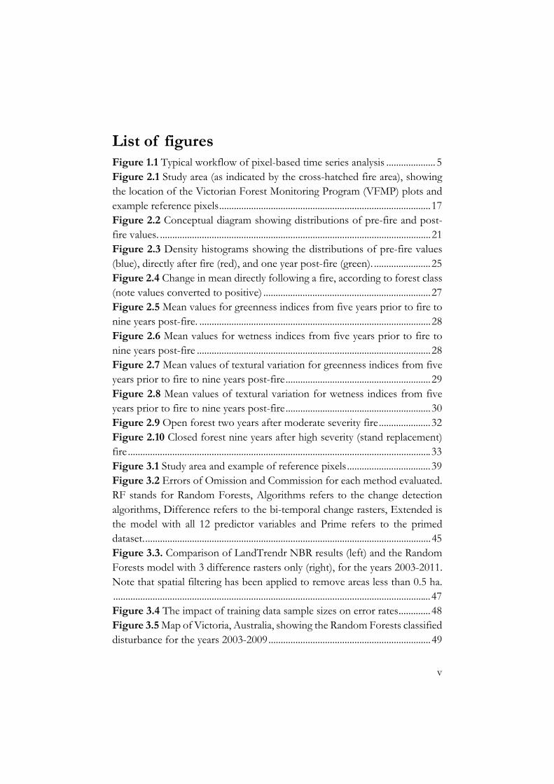
List of figures Figure 1.1 Typical workflow of pixel-based time series analysis .................... 5 Figure 2.1 Study area (as indicated by the cross-hatched fire area), showing the location of the Victorian Forest Monitoring Program (VFMP) plots and example reference pixels ...................................................................................... 17 Figure 2.2 Conceptual diagram showing distributions of pre-fire and post-fire values. .............................................................................................................. 21 Figure 2.3 Density histograms showing the distributions of pre-fire values (blue), directly after fire (red), and one year post-fire (green). ....................... 25 Figure 2.4 Change in mean directly following a fire, according to forest class (note values converted to positive) .................................................................... 27 Figure 2.5 Mean values for greenness indices from five years prior to fire to nine years post-fire. .............................................................................................. 28 Figure 2.6 Mean values for wetness indices from five years prior to fire to nine years post-fire ............................................................................................... 28 Figure 2.7 Mean values of textural variation for greenness indices from five years prior to fire to nine years post-fire ........................................................... 29 Figure 2.8 Mean values of textural variation for wetness indices from five years prior to fire to nine years post-fire ........................................................... 30 Figure 2.9 Open forest two years after moderate severity fire ..................... 32 Figure 2.10 Closed forest nine years after high severity (stand replacement) fire ........................................................................................................................... 33 Figure 3.1 Study area and example of reference pixels .................................. 39 Figure 3.2 Errors of Omission and Commission for each method evaluated. RF stands for Random Forests, Algorithms refers to the change detection algorithms, Difference refers to the bi-temporal change rasters, Extended is the model with all 12 predictor variables and Prime refers to the primed dataset. .................................................................................................................... 45 Figure 3.3. Comparison of LandTrendr NBR results (left) and the Random Forests model with 3 difference rasters only (right), for the years 2003-2011. Note that spatial filtering has been applied to remove areas less than 0.5 ha. ................................................................................................................................. 47 Figure 3.4 The impact of training data sample sizes on error rates ............. 48 Figure 3.5 Map of Victoria, Australia, showing the Random Forests classified disturbance for the years 2003-2009 .................................................................. 49

vi
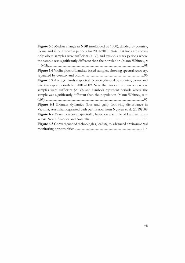
Figure 3.6 Area of forest disturbed each year between 1989 and 2017 in Victoria, Australia ................................................................................................. 50 Figure 3.7 Mean decrease in accuracy plot from the Random Forests model with 12 predictors ................................................................................................. 52 Figure 4.1 Overview of the spectral disturbance and recovery mapping workflow ................................................................................................................ 59 Figure 4.2 Study area, showing large wildfires that occurred between 2002 and 2009, overlaid on bioregions, within the state of Victoria, Australia. ... 60 Figure 4.3 Example of 600 m × 600 m patches, showing disturbance, recovery and the corresponding correlations. The top row shows a patch with strong positive correlation (i.e., higher disturbance magnitude equals longer recovery), while the bottom row shows a patch with strong negative correlation (i.e., higher disturbance magnitude equals shorter recovery). .... 65 Figure 4.4 Example of the derived spectral disturbance (panel A) and recovery (panel B) maps for the 2003 Bogong fire ......................................... 68 Figure 4.5 Map showing patch-level disturbance-recovery correlations. Smoothing has been applied to the state map. ................................................. 71 Figure 4.6 Density histograms of patch level correlations for each bioregion ................................................................................................................................. 72 Figure 4.7 Patch level correlations of the 5 most prominent Ecological Vegetation Divisions within the South Eastern Highlands bioregion .......... 73 Figure 4.8 Patch level correlations in each EVD, displayed as a proportional representation ........................................................................................................ 74 Figure 5.1 Temperate and boreal related biomes, according to the World Wildlife Fund (WWF) classification, intersected with the countries and regions used in this study .................................................................................... 84 Figure 5.2 Area burned by fires greater than 200 ha, between 2001 and 2018, as detected by the MODIS burned area product (MCD64A1). Also shown are country averages (dashed grey line) and Theil-Sen slopes (solid black line). Note that the scales on the y-axis are different. ............................................... 92 Figure 5.3 Average fire size (ha), between 2001 and 2018, as detected by the MODIS burned area product (MCD64A1), sub-divided by country, biome and into three-year periods. Note that data is only displayed for cases with at least 5 time-periods which each contain at least 30 fires. ............................... 93 Figure 5.4 Violin plots of Landsat-based samples, showing the change in NBR (multiplied by 1000), separated by country and biome. ........................ 94
vii
Figure 5.5 Median change in NBR (multiplied by 1000), divided by country, biome and into three-year periods for 2001-2018. Note that lines are shown only where samples were sufficient (> 30) and symbols mark periods where the sample was significantly different than the population (Mann-Whitney, α = 0.05). ................................................................................................................... 95 Figure 5.6 Violin plots of Landsat-based samples, showing spectral recovery, separated by country and biome. ........................................................................ 96 Figure 5.7 Average Landsat spectral recovery, divided by country, biome and into three-year periods for 2001-2009. Note that lines are shown only where samples were sufficient (> 30) and symbols represent periods where the sample was significantly different than the population (Mann-Whitney, α = 0.05). ....................................................................................................................... 97 Figure 6.1 Biomass dynamics (loss and gain) following disturbance in Victoria, Australia. Reprinted with permission from Nguyen et al. (2019) 108 Figure 6.2 Years to recover spectrally, based on a sample of Landsat pixels across North America and Australia ................................................................ 111 Figure 6.3 Convergence of technologies, leading to advanced environmental monitoring opportunities .................................................................................. 114

viii
List of tables Table 2.1 Native forest structural classes in Australia .................................... 16 Table 2.2 Landsat spectral indices used in this paper, and a selection of pixel-based time series studies using these indices (band numbers refer to Landsat TM and ETM+ bands). ....................................................................................... 19 Table 2.3 Number of reference pixels in each forest class used in this study ................................................................................................................................. 22 Table 2.4 Post-fire response of each index, shown as a standardized change in mean, percentage overlap, and relative change in standard deviation, with best results indicated in bold. .............................................................................. 26 Table 2.5 Average number of years to recover. .............................................. 29 Table 3.1 Results of manually interpreted reference pixels ........................... 40 Table 3.2 Errors of omission and commission for each breakpoint detection algorithm, the simple aggregation ensembles, and the Random Forests ensembles ............................................................................................................... 46 Table 4.1 Main Ecological Vegetation Divisions (EVDs) in the South Eastern Highlands bioregion relevant to this study, along with corresponding major Ecological Vegetation Classes (EVCs), average rainfall and elevation. ................................................................................................................................. 66 Table 4.2 Average disturbance magnitude (change in NBR) and standard deviation by bioregion ......................................................................................... 67 Table 4.3 Average spectral recovery length and standard deviation, plus correlations between disturbance magnitude and recovery, by bioregion ... 69 Table 4.4 Average patch level correlations for each bioregion and the entire state of Victoria. Note that the percentage of correlations is based on α = 0.005, which means that positive correlations are typically > 0.15, while negative are < -0.15. ............................................................................................. 70 Table 4.5 Average correlations for each Ecological Vegetation Division. Note that the percentage of correlations is based on α = 0.005, which means that positive correlations are typically > 0.15, while negative are < -0.15. .. 72 Table 5.1 Area burned by fires greater than 200 ha per country and biome in the period 2001-2018, as detected by the MODIS burned area product (MCD64A1). Also, Thiel-Sen slope results (yearly percentage in relation to average annual area burned), with significant trends (Mann-Kendall, α = 0.05) marked with *. ....................................................................................................... 90

ix
Table A1: Total burned area and average change in NBR (×1000) for each fire event (Chapter 4) ......................................................................................... 135 Table A2: Average recovery length for each fire event (Chapter 4) .......... 136 Table A3: Mann-Whitney U tests between pairs of bioregions (Chapter 4) ............................................................................................................................... 137 Table A4: Mann-Whitney U tests between pairs of Ecological Vegetation Divisions (Chapter 4) ......................................................................................... 138 Table A5: Patch-level correlations between disturbance magnitude, recovery and elevation. Positive correlations are > 0.15, while negative are < -0.15. ............................................................................................................................... 139

x

1
Chapter 1: General Introduction The aim of this research is to develop techniques to strengthen the use of Earth observation for sustainable forest management, particularly in relation to monitoring forest disturbance and recovery across large areas. This chapter provides an overview of the problem, introduces the concept of satellite-based time series and outlines the structure of the subsequent chapters in this thesis.

GeneralIntroduction
2
1.1 Forest monitoring and reporting Almost one third of the Earth’s land is covered by forests (Keenan et al., 2015). Forests generate clean air and water, cycle carbon and nutrients, and provide resources (such as timber, food and fuel) for billions of people. In addition, forests contain more than three-quarters of the world’s terrestrial biodiversity and absorb roughly 2 billion tonnes of carbon each year (FAO, 2018). The importance of forests to life on Earth cannot be overstated.
Increasingly, governments are aiming to manage forest resources sustainably, in ways that balance economic, ecological and social factors. While the notion of sustainable forest management itself is not new (Macdicken et al., 2015), it gained considerable momentum at an international level following the Rio Earth Summit in 1992 (Montréal Process, 2009). Across the world, various levels of government have forest monitoring and reporting obligations, often enshrined in legislation, policies and international agreements. In Australia, for example, all states and territories, and the Australian Government have legislation supporting sustainable forest management. In addition, under a National Forest Policy Statement, Australia is committed to reporting on the state of its forests every five years. This data is also used in international reports, such as the global Forest Resources Assessment, as prepared by the Food and Agriculture Organization of the United Nations (MIG and NFISC, 2018).
Sustainable forest management is also integral to achieving the United Nations Sustainable Development Goals (SDGs); a recent report details the contributions that forests make to 28 targets relating to 10 of the 17 SDGs (FAO, 2018). Protecting biodiversity through forest conservation and restoration is also critical to meeting the Aichi Biodiversity Targets (www.cbd.int/sp/targets/). Forests also play an essential role in combating climate change and limiting global warming, recognised by initiatives such as the United Nations program for Reducing Emissions from Deforestation and Forest Degradation (www.un-redd.org).
A key aspect of sustainable forest management is the use of criteria and indicators for forest management and reporting. Criteria are broad themes of forest values, while indicators are measurable aspects of these criteria.

Chapter1
3
International collaborations, such as the Montréal Process, have been integral to the development of common criteria and indicators, now used throughout the world (Montréal Process, 2009). Recognised under “Criterion 3: maintenance of ecosystem health and vitality” is a forest’s ability to adapt to and recover from disturbances, both biotic (e.g., disease, insects, invasive species) and abiotic (e.g., fire, storm, land clearance). Changes beyond reference conditions may threaten a forest’s health and vitality (Montréal Process, 2009).
Forest disturbance and subsequent recovery (or regeneration) is, in many ways, a natural process essential to healthy forest systems. Dead and decaying trees, whether standing or fallen, stimulate biodiversity and provide habitat for many species (Senf et al., 2018). However, according to Thom and Seidl, (2016), the benefits of disturbance on biodiversity are often out-weighed by negative impacts to other ecosystem services (e.g., clean air, water and food). In the current day, it is difficult to distinguish between natural and anthropogenic disturbances, given the influence that humans inflict on fire regimes, invasive species, exotic pathogens, and climate change. Complex ecological feedback loops mean that forests are in a constant state of flux. Nonetheless, changes to disturbance regimes (i.e., type, frequency, severity, spatial extent and pattern), whether anthropogenic or not, may considerably alter forest ecosystems (Thom and Seidl, 2016).
Increasingly, scientists and land managers are regarding the Earth as an interconnected system (Steffen et al., 2007), of which forests are an essential element. While global initiatives promoting sustainable forest management provide necessary policy directions, implementation of meaningful actions remains challenging. The 2030 Agenda towards achieving the SDGs recognises that “if you can’t measure it, you can’t manage it” (Paganini et al., 2018). Earth observation satellites provide solutions for large-area and global monitoring. However, the potential of satellites is yet to be fully realised, especially in ecological applications. This is due in part to inconsistent data, methods and capabilities, exacerbated by a lack of communication between the ecology and remote sensing communities (Skidmore et al., 2015). In addition, while the value of satellite Earth observation has long been recognised in a spatial sense, the temporal capacity has been underutilised. It

GeneralIntroduction
4
is the ability of satellites to consistently observe ecosystems over time that offers an improved understanding of ecological dynamics (Kennedy et al., 2014).
1.2 Satellite Earth observation time series Satellite Earth observation allows landscapes to be assessed and monitored over large extents, consistently across time and space. Wall-to-wall coverage, along with recent improvements in computing power, has led to unprecedented interest in large-area applications. Although there are numerous Earth observation satellites in operation today, the Landsat program stands alone in terms of its temporal depth, radiometric calibration and open access (Wulder et al., 2018). The Landsat family of satellites have been imaging the Earth for over four decades. Since the mid to late 80s, Landsat has provided multispectral data at a 30 m spatial resolution and 16 day temporal resolution; characteristics which are suitable for large-area forest monitoring.
In 2008, the United States Geological Survey (USGS) made their Landsat archive free and accessible, a decision that revolutionised Earth sciences (Wulder et al., 2012). This was followed by the Landsat Global Archive Consolidation (LGAC) initiative in 2010, which aimed to consolidate Landsat data from receiving stations throughout the world into a central repository (Wulder et al., 2016). The USGS now holds more than 8 million unique Landsat scenes.
Because of Landsat’s unrivalled position in Earth observation, considerable research has been undertaken to make the data suitable for time series analysis, including the development of standardized processes for radiometric, geometric, and atmospheric correction, such as the Landsat Ecosystem Disturbance Adaptive Processing System (LEDAPS) algorithm (Schmidt et al., 2013). The resultant ‘surface reflectance’ products make it possible to track each pixel through time. While there are other surface reflectance algorithms (e.g., Li et al., 2012), LEDAPS is the most common, and is therefore used in this research. Figure 1.1 shows a typical workflow of pixel-based time series analysis, which is subsequently summarised.

Chapter1
5
Figure 1.1 Typical workflow of pixel-based time series analysis
1.2.1 Image compositing
Cloud-cover is a constant issue with optical remote sensing. To deal with clouds and other data gaps (e.g., Landsat 7’s Scan-Line-Corrector (SLC) failure), along with the ability to undertake studies across many Landsat scenes, it has become common practice to build image composites, constructed out of multiple images. Typically, clouds and cloud shadows are masked prior to compositing. Many cloud masking algorithms have been

GeneralIntroduction
6
proposed (for a review, see White et al., 2014). One of the most widely used, and provided with USGS Landsat products, is that of Zhu and Woodcock (2012). Referred to as Fmask, the authors state its accuracy “as high as 96.4%”.
Best-available-pixel composites have become integral to many time series studies (White et al., 2014). Several different compositing rules have been used. For example, selecting the greenest pixel by taking the maximum value of a spectral index like NDVI (Holben, 1986). An alternate method is to select a target date and use the first clear pixel closest to that date within a certain time period (Kennedy et al., 2010). Recently, more sophisticated rules have been proposed, where pixels are ranked based on day-of-year in addition to factors such as atmospheric opacity and presence/closeness to cloud or shadow (White et al., 2014). A method proposed by Flood (2013) uses the ‘medoid’ across all Landsat bands, whereby the pixel with the smallest sum of the distances to all the other pixels is selected. Therefore, the pixel is always a true value, and the relationships between bands are preserved. The medoid is currently the preferred compositing method in the Google Earth Engine implementation of LandTrendr (Kennedy et al., 2018b).
1.2.2 Change detection algorithms
There are many different Landsat time series approaches in the literature. In a comprehensive review, Zhu (2017) identified upwards of 50 different ‘change detection’ algorithms, which he grouped into 6 broad categories, based on the mathematical approaches employed. These include thresholding, differencing, segmentation, trajectory classification, statistical boundary, and regression. Most are based at the pixel level and tend to either use all available images (e.g., Eklundh and Jönsson, 2015; Verbesselt et al., 2010a; Zhu and Woodcock, 2014) or one image per year (e.g., Hermosilla et al., 2015; Kennedy et al., 2010).
Change detection algorithms typically aim to extract meaningful changes (e.g., a disturbance event) and/or trends (e.g., forest recovery) from each pixel’s temporal trajectory (Figure 1.1). Algorithms have been employed to create accurate maps of forest disturbance over time, due to various agents such as fire, logging and insects (Huang et al., 2010; Kennedy et al., 2012; Senf et al.,

Chapter1
7
2015). Modern computing power has enabled studies across extremely large areas; for example: the entire forest estate of Canada (Coops et al., 2018), the conterminous United States (Cohen et al., 2016), and eastern Europe (Potapov et al., 2015).
1.2.3 Spectral indices and ensemble approaches
Most change detection algorithms operate at the pixel level in 2 dimensions, where the x-axis equals time and the y-axis is either an individual band or a spectral index (computed from multiple bands). Different bands and indices are sensitive to different aspects of vegetation cover. Indices most commonly used in forest-based Landsat time series include the Normalised Difference Vegetation Index or NDVI (Tucker, 1979), the Normalised Burn Ratio or NBR (Key and Benson, 2006) and the various Tasseled Cap components (Crist and Cicone, 1984). NBR has been used widely (Hermosilla et al., 2015a; Kennedy et al., 2010), due to its ability both to capture change and accurately represent forest recovery (White et al., 2018). Some studies used a spectral band (e.g., band 5) rather than an index (Schroeder et al., 2011). Huang et al. (2010) used all bands, converted to standardised scale (z-score) and integrated to form a one-dimensional output. The different components of the Tasseled Cap transformation have been found to be sensitive to different types of disturbance. For example, Senf et al. (2015) found that Greenness was useful in detecting Western Spruce Budworm disturbance, but Wetness and Brightness were better indicators of Mountain Pine Beetle disturbance.
Cohen et al. (2017a) recently showed that different indices and time series methods produce results which vary considerably. Thus, instead of relying on one method/index, there has been a recent shift towards using ensemble approaches (Cohen et al., 2017b; Haywood et al., 2016; Healey et al., 2018; Schultz et al., 2016c), where multiple indices are used in conjunction with a machine learning classifier (e.g., Random Forests) and robust reference data, to improve disturbance classification.
1.2.4 Reference data
Many change detection algorithms do not necessarily require reference data to function. However, reference data is important for validation and calibration purposes. Cohen et al. (2010) developed an automated approach

GeneralIntroduction
8
for collecting human interpreted reference data called TimeSync. A similar approach was adopted by Soto-Berelov et al. (2017) in the state of Victoria, Australia. In a recent study, Senf et al. (2018) did not use a change detection algorithm at all; instead, the authors used TimeSync to interpret 24,000 pixel samples to assess canopy mortality across Europe. Reference data is also required for machine learning ensemble approaches and supervised classifications. For example, in Washington, USA, Kennedy et al. (2015) used a change detected algorithm called LandTrendr to detect changes, which were subsequently classified into three classes: urbanization, forest management, and natural. In the Central Highlands in Victoria, Australia, Haywood et al. (2016) used the BFAST algorithm to detect changes, which were then classified into fire and logging disturbances at different severity levels.
1.2.5 Spectral recovery
Recently, researchers have moved beyond using Landsat time series to detect forest disturbances only, and are now using it to also study forest recovery (Kennedy et al., 2012; Pickell et al., 2016; White et al., 2018). Forest recovery following disturbance is a complex process, with numerous successional stages. It begins with an initial re-establishment of vegetation and progresses through to a gradual return of forest structural characteristics (White et al., 2017). Although passive sensors such as Landsat cannot directly measure forest structure, spectral indices using the SWIR bands (e.g., NBR) have been shown to correlate highly with lidar derived structural measurements (White et al., 2018).
1.3 This research This research attempts to bridge the gap between complex remote sensing practices and useful information; that is, information which is meaningful, accessible and relevant to land managers and policy makers. The core chapters in this thesis present elements of a tool chain, used to translate big data into scientifically robust information. The outputs of various techniques are used in case studies, to explore ecological elements of forest disturbance (particularly fire) and subsequent recovery. In particular, this research aims to exploit the potential of the 30+ year Landsat image archive to produce

Chapter1
9
evidence-based outputs that can support forest monitoring and reporting activities across large areas.
1.3.1 Research objectives
The main objectives of this research are to:
1) Assess the potential of a number of Landsat-based spectral indices in their ability to detect fire disturbance and characterise subsequent forest recovery in southeast Australian forests
2) Explore the benefits of using an ensemble of spectral indices, in conjunction with human interpreted reference data and machine learning, to produce forest disturbance maps
3) Examine the relationship between spectral disturbance magnitude and recovery length, to determine: a) Whether a statistical association exists, and how well it can be
characterised using Landsat time series b) How the association varies across different forest types
4) Investigate fire disturbance and forest recovery in boreal and temperate forests worldwide, using the MODIS and Landsat image archives, to: a) Explore trends in burned area, fire severity (change in NBR) and
forest recovery lengths (as measured spectrally) b) Establish similarities and differences between similar forest types in
different countries c) Determine the transferability and scalability of methods developed in
the previous objectives.
1.3.2 Study area
The study area for chapters 2, 3 and 4 of this thesis is the state of Victoria, Australia. Or, more specifically, the 8.2 million ha of forests in Victoria, which cover approximately one third of the state (Soto-Berelov et al., 2018b). In chapter 5, the study area was extended to temperate and boreal forests across the world; in particular, Montreal Process countries that regularly experience forest fires (Australia, Canada, Chile, China, Russia and the USA), along with southern Europe. Boreal and temperate biomes were based on the classification of Olson et al. (2001). In total, around 50% of the world’s forests were analysed (~2 billion ha). Given the different study areas used for

GeneralIntroduction
10
different parts of this research, further information is provided in each of the core chapters.
1.3.3 Outline of thesis
This thesis comprises six chapters: a general introduction, four core research chapters – each based on a peer-reviewed journal paper – and a synthesis.
Chapter 1 introduced the concept of sustainable forest management and how satellite remote sensing, particularly when used in time series, can contribute.
Chapter 2 examines eight different Landsat-based spectral vegetation indices and assesses their sensitivity to fire disturbance and forest recovery in southeast Australian forests.
Chapter 3 explores whether an ensemble approach, using multiple indices and a Random Forests classifier, can produce more accurate maps of forest disturbance than individual time series algorithms.
Chapter 4 delves deeper into the ecological applications of Landsat time series, by exploring whether a greater disturbance magnitude equates to a longer recovery length in different forest types in southeast Australia.
Chapter 5 takes the lessons learned from chapters 2-4 to produce a global study looking at fire disturbance and subsequent forest recovery in the boreal and temperate forests across the world. This chapter demonstrates a robust and straightforward method for analysing fire disturbance and forest recovery trends, which can improve forest monitoring and reporting.
Chapter 6 provides an overview of the major findings outlined in the thesis, places them in a broader context, and explores future opportunities to capitalise on the recent convergence of technologies and data availability in Earth observation.

11
Chapter 2: Using Landsat spectral indices in time series to assess wildfire disturbance and recovery1
1 This chapter is based on: Hislop, S., Jones, S., Soto-Berelov, M., Skidmore, A., Haywood, A., Nguyen, T.H., 2018. Using Landsat spectral indices in time-series to assess wildfire disturbance and recovery. Remote Sens. 10, 1–17. https://doi.org/10.3390/rs10030460

Landsatspectralindices
12
Abstract Freely available Landsat data stretching back four decades, coupled with advances in computer processing capabilities, has enabled new time series techniques for analysing forest change. Typically, these methods track individual pixel values over time, through the use of various spectral indices. This study examines the utility of eight spectral indices, in their ability to characterise fire disturbance and recovery in sclerophyll forests, in order to determine their relative merits in the context of Landsat time series. Although existing research into Landsat indices is comprehensive, this study presents a new approach for evaluating indices without the need of detailed field information, by comparing the distributions of pre and post-fire pixels using Glass’s delta. Results showed that, in the sclerophyll forests of southeast Australia, common indices, such as the Normalized Difference Vegetation Index (NDVI) and the Normalized Burn Ratio (NBR), both accurately captured wildfire disturbance in a pixel-based time series approach, especially if images from soon after the disturbance were available. However, for tracking forest regrowth and recovery, indices such as NDVI (which typically capture canopy ‘greenness’) were not considered reliable, with values returning to pre-fire levels in 3-5 years. In comparison, indices that are more sensitive to forest moisture and structure, such as NBR, indicated much longer (8-10 years) recovery timeframes. This finding is consistent with studies conducted in other forest types. This study also found that additional information regarding forest condition, particularly in relation to recovery, may be available in lesser-known indices, such as NBR2, as well as in textural indices incorporating spatial variance. With Landsat time series being increasingly used in forest monitoring applications, it is essential to understand the advantages and limitations of the various indices that these methods rely on.

Chapter2
13
2.1 Introduction The opening of the Landsat archive in 2008, along with the advances in computer processing, has led to a plethora of new and novel applications exploiting Landsat time series (Wulder et al., 2012). Commonly, in the forest domain, these studies look to establish disturbance and recovery histories, following events such as wildfire, logging, and insect damage (Kennedy et al., 2010; Schroeder et al., 2011; Senf et al., 2015). Using a time series, rather than image pairs, allows for change to be differentiated from background noise, whilst also capturing longer-term ecological trends (Kennedy et al., 2010).
Methods for characterizing forest dynamics (abrupt changes and longer-term trends) using time series differ, but a point of similarity is the use of spectral indices. Spectral indices convert multi-spectral satellite data into a single component, so individual pixels can be tracked through time. Spectral indices also have an advantage over single bands by amplifying desired effects (e.g., changes in vegetation condition) and reducing unwanted features, such as atmospheric and topographic noise (Matsushita et al., 2007). There are numerous spectral indices in the literature. However, when considering those commonly used in Landsat derived pixel-based time series, the field narrows significantly. Frequently used is the Normalized Difference Vegetation Index (NDVI; Tucker, 1979). NDVI is a measure of photosynthetic biomass, and has been shown to correlate with ecological parameters, such as the fraction of green vegetation cover (Verbesselt et al., 2010a) and leaf area index (Wang et al., 2005). NDVI is sensitive to changes in vegetation condition and has been shown to accurately detect forest disturbances. However, it is considered to be less adept in representing forest recovery, due to grasses and other non-woody vegetation colonizing a site after a disturbance, and consequently returning the NDVI signal to its pre-disturbance state (Pickell et al., 2016). In areas of sparse vegetation, NDVI can be adversely affected by soil reflectance. To correct for this, Huete developed the Soil Adjusted Vegetation Index (SAVI), which incorporates a soil correction factor into the NDVI formula (Huete, 1988).
Indices using short-wave infrared (SWIR) bands are commonly used in Landsat time series, as these wavelengths are often more sensitive to forest structure, moisture, shadowing, and vegetation density (Schroeder et al.,

Landsatspectralindices
14
2011). The Normalized Burn Ratio (NBR) is a ratio of the near-infrared and second SWIR band (2.08-2.35 μm), and was developed by Key and Benson (2006) to identify burned areas following fire and provide a quantitative measure of burn severity. Several authors have found NBR to correlate highly with field-based measurements in forest ecosystems (Cocke et al., 2005; Epting et al., 2005; Parker et al., 2015); however, Roy et al. (2006) suggest caution when using NBR for burn severity mapping as their investigations indicated sub-optimal results. In Landsat time series, NBR is used extensively, and has proven adept at characterizing forest dynamics in the USA (Kennedy et al., 2012) and Canada (White et al., 2017). Similar to NBR is the Normalized Difference Moisture Index (NDMI), which uses the near-infrared with the first SWIR band (1.55-1.75 μm). NDMI is sometimes favoured for tracking disturbances other than fire, and was used by Goodwin et al. (2008) for classifying areas that were disturbed by the Mountain Pine Beetle in western Canada. NBR2 is another variation of a ratio/difference index, contrasting the two Landsat SWIR bands. It is provided as a standard product by the United States Geological Survey (USGS) but has been rarely used in the literature. Storey et al. (2016) found it useful for post-fire recovery assessment in chamise chaparral vegetation in southern California, while Stroppiana et al. (2012) used it as part of an ensemble to map burned areas.
The Tasseled Cap (TC) transformation of Landsat Multispectral Scanner (MSS) data was first presented by Kauth and Thomas in 1976, and was later adapted by Crist and Cicone for Landsat TM data (Crist and Cicone, 1984). The various components of TC are created via linear transformations using defined coefficients. In simplified terms, Brightness (TCB) represents the overall brightness of all bands, Greenness (TCG) is a contrast between the visible and near-infrared bands, and Wetness (TCW) is a contrast of the visible and near-infrared with the SWIR bands, making it sensitive to soil and plant moisture (Crist and Cicone, 1984). TC Angle (TCA; Powell et al., 2010) is calculated as the arctan of TCG/TCB and describes the vegetation cover within the TCB-TCG spectral plane (Pflugmacher et al., 2012). Various time series studies have shown success with TC components. For instance, Senf et al. (2015) used TC components to track insect disturbance in British Columbia, Canada, and found that TCG was useful for detecting Western

Chapter2
15
Spruce Budworm disturbance, whereas TCW and TCB were better indicators of Mountain Pine Beetle disturbance.
The time series method, and the index (or indices) used, can significantly alter the outcomes of a study, as highlighted recently by Cohen et al. (2017b). Often, studies evaluating spectral indices look to establish the strength of the relationship between the index and field data (Cocke et al., 2005). An alternative approach, especially when field data are not available, is to use human-interpreted reference data. Recently, Schultz et al. (2016b) assessed eight spectral indices in their ability to detect deforestation in the tropics, using manually interpreted reference pixels for training and validation. The challenge with using field data and human interpreted imagery to train or validate models is that the data needs to be both spatially representative of the study area and temporally relevant (i.e., collected at appropriate time intervals). Many Landsat time series studies are retrospective investigations covering large areas, and field data does not exist. Where ancillary data is available, it is more likely to indicate forest disturbance (e.g., maps of fire extent and severity) than forest recovery, which would require multiple data collections over many years. One of the strengths of satellite Earth observation (especially Landsat) is the consistent re-visit cycles, which enables the characterization of trends, such as forest recovery.
This study adds several insights to the existing body of literature on spectral indices. Firstly, it presents a simple and robust method for assessing and comparing indices using Glass’s delta, which is suitable where limited or no field data are available. Secondly, it looks at how various indices respond to fire disturbance and recovery in sclerophyll forests, which are the dominant forest type in Australia, but also exist elsewhere in the world. Thirdly, it assesses indices in the context of Landsat time series, but independently of a specific change detection algorithm.
2.2 Materials and methods
2.2.1 Study area
The study area contains over three million hectares of public forest in the eastern half of Victoria, Australia (Figure 2.1). This area was chosen because
Landsatspectralindices
16
it has high ecological and economic importance, and it recently experienced three major wildfire events in the space of six years. The area consists primarily of sclerophyll forests, tending to wet in some areas and dry in others. At the wetter end, trees can attain heights over 75 m, while at the dryer end, trees are typically shorter than 40 m (Viridans, 2017). The study area falls primarily within three bioregions – the Victorian Alps and the Northern and Southern Highlands (IBRA, 2017). The Alps have mild summers and cool winters, reach elevations up to 2000 m, and typically experience over 1400 mm of annual precipitation. The Highlands are located on both the northern and southern sides of the Alps, at elevations between 200 m and 1300 m, and typically experience annual rainfall between 500 and 1200 mm (Viridans, 2017). Forests in Australia are also divided by structural classes (Table 2.1; refer to Mellor and Haywood, (2010) for details).
Table 2.1 Native forest structural classes in Australia
Tree Height (m) Canopy Cover (%)
Low (<10) Woodland (<50)
Medium (10-30) Open (50-80)
Tall (>30) Closed (>80)
In 2003, wildfires in the northeast of Victoria burned over 1.3 million ha of forest. Three years later, over the summer of 2006-2007, major wildfires again burned a further 1 million ha of forest, mostly southwest of the 2003 fires. In February 2009, the devastating ‘Black Saturday’ fires burned a further 400,000 ha across the state of Victoria (Attiwill and Adams, 2013), much of it in the Central Highlands region. Figure 2.1 indicates the extent of the burned area, which forms the study area for this research.
Chapter2
17
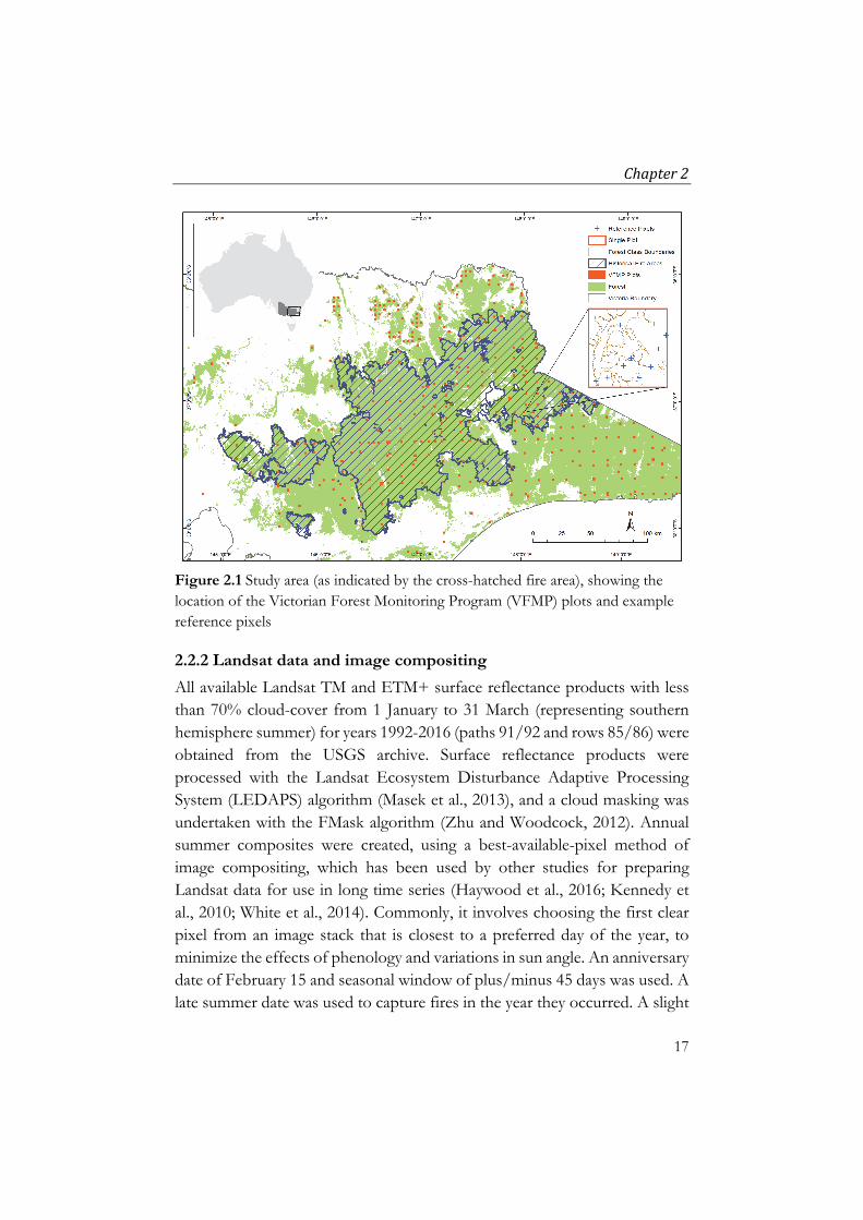
Figure 2.1 Study area (as indicated by the cross-hatched fire area), showing the location of the Victorian Forest Monitoring Program (VFMP) plots and example reference pixels
2.2.2 Landsat data and image compositing
All available Landsat TM and ETM+ surface reflectance products with less than 70% cloud-cover from 1 January to 31 March (representing southern hemisphere summer) for years 1992-2016 (paths 91/92 and rows 85/86) were obtained from the USGS archive. Surface reflectance products were processed with the Landsat Ecosystem Disturbance Adaptive Processing System (LEDAPS) algorithm (Masek et al., 2013), and a cloud masking was undertaken with the FMask algorithm (Zhu and Woodcock, 2012). Annual summer composites were created, using a best-available-pixel method of image compositing, which has been used by other studies for preparing Landsat data for use in long time series (Haywood et al., 2016; Kennedy et al., 2010; White et al., 2014). Commonly, it involves choosing the first clear pixel from an image stack that is closest to a preferred day of the year, to minimize the effects of phenology and variations in sun angle. An anniversary date of February 15 and seasonal window of plus/minus 45 days was used. A late summer date was used to capture fires in the year they occurred. A slight

Landsatspectralindices
18
penalty (five days) was applied to ETM+ images with Scan Line Corrector errors (SLC-off), so that preference was given to TM data if available. This resulted in a time series stack of 25 years with over 98% coverage.
2.2.3 Candidate reference pixels
Fire maps maintained by the state of Victoria’s land management agency (Department of Environment Land Water and Planning, 2017) were used to indicate the general extent of the three large fires. Candidate reference pixels were chosen via a systematic sampling process based on the Victorian Forest Monitoring Program (VFMP) plot network (Haywood and Stone, 2017). The VFMP plot network consists of 786 plots (2 km × 2 km) that are distributed throughout public land in Victoria, stratified by bioregion and land tenure. In each plot, 10 random pixels were selected (resulting in 7860 pixels), and a team of six worked to manually interpret each pixel to establish its disturbance history (Figure 2.1 shows an example of the reference pixel sampling method). This was achieved by interrogating multiple lines of evidence, such as state fire records and high-resolution imagery from Google Earth. Quality assurance was performed by an independent operator, who assessed 10% of all the pixels to evaluate the accuracy of the dataset (see Soto-Berelov et al. (2017) for details). A total of 1391 pixels fell within the broad fire boundaries. Of these, 1056 were classified as being disturbed by one or more of the three wildfires, and were subsequently used for the bulk of the analysis presented in this paper. In the section investigating different forest classes, an additional 5000 random pixels (with a minimum distance of 100 m) were selected inside the VFMP plots that fell within the fire history polygons; this ensured an adequate number of samples in each class. Visual inspection of the imagery indicated that, on balance, the majority of these pixels were fire affected.

Chapter2
19
Table 2.2 Landsat spectral indices used in this paper, and a selection of pixel-based time series studies using these indices (band numbers refer to Landsat TM and ETM+ bands).
Greenness Indices Formula Pixel-Based Time-
Series Studies
Normalized Difference Vegetation Index (NDVI) 𝑵𝑫𝑽𝑰
𝑵𝑰𝑹 𝑹𝑬𝑫𝑵𝑰𝑹 𝑹𝑬𝑫
(Dutrieux et al., 2015; Kennedy et al., 2010; Schmidt et al., 2015;
Vogelmann et al., 2012)
Soil Adjusted Vegetation Index (SAVI) 𝑺𝑨𝑽𝑰
𝑵𝑰𝑹 𝑹𝑬𝑫𝑵𝑰𝑹 𝑹𝑬𝑫 𝟎. 𝟓
𝟏 𝟎. 𝟓 (Sonnenschein et al., 2011)
Tasseled Cap Greenness (TCG)
−0.1603(band 1) − 0.2819(band 2) − 0.4934(band 3) + 0.7940(band 4) − 0.0002(band 5) − 0.1446(band 7)
(Frazier et al., 2015; Hudak et al., 2013; Senf et
al., 2015)
Tasseled Cap Angle (TCA) 𝑻𝑪𝑨 𝒂𝒓𝒄𝒕𝒂𝒏𝑻𝑪𝑮𝑻𝑪𝑩
(Haywood et al., 2016;
Kennedy et al., 2012; Schroeder et al., 2011)
Wetness Indices
Normalized Burn Ratio (NBR) 𝑵𝑩𝑹𝑵𝑰𝑹 𝑺𝑾𝑰𝑹𝒃𝒂𝒏𝒅𝟕
𝑵𝑰𝑹 𝑺𝑾𝑰𝑹𝒃𝒂𝒏𝒅𝟕
(Huang et al., 2010; Kennedy et al., 2010; Senf
et al., 2015)
Normalized Difference Moisture Index (NDMI) 𝑵𝑫𝑴𝑰
𝑵𝑰𝑹 𝑺𝑾𝑰𝑹𝒃𝒂𝒏𝒅𝟓
𝑵𝑰𝑹 𝑺𝑾𝑰𝑹𝒃𝒂𝒏𝒅𝟓
(DeVries et al., 2015; Dutrieux et al., 2016;
Goodwin et al., 2008)
Tasseled Cap Wetness (TCW) 0.0315(band 1) + 0.2021(band 2) + 0.3102(band 3) + 0.1594(band 4) − 0.6806(band 5) − 0.6109(band 7)
(Frazier et al., 2015; Hudak et al., 2013;
Kennedy et al., 2010; Senf et al., 2015)
Normalized Burn Ratio 2 (NBR2)
𝑵𝑩𝑹𝟐𝑺𝑾𝑰𝑹𝒃𝒂𝒏𝒅𝟓 𝑺𝑾𝑰𝑹𝒃𝒂𝒏𝒅𝟕
𝑺𝑾𝑰𝑹𝒃𝒂𝒏𝒅𝟓 𝑺𝑾𝑰𝑹𝒃𝒂𝒏𝒅𝟕 (Storey et al., 2016)
Tasseled Cap Brightness (TCB) (used to calculate TCA)
0.2043(Band 1) + 0.4158(band 2) + 0.5524(band 3) + 0.5741(band 4) + 0.3124(band 5) + 0.2303(band 7)
(Frazier et al., 2015; Haywood et al., 2016;
Hudak et al., 2013; Senf et al., 2015)
2.2.4 Landsat spectral indices
From the composite Landsat images, the spectral indices shown in Table 2.2 were computed. These included NDVI, SAVI, NBR, NDMI, NBR2, and the Tasseled Cap indices (TCG, TCW and TCA). TCB was not included due to its unpredictable nature (sometimes increasing, sometimes decreasing, following fire); however, it was used to calculate TCA. Landsat TM and ETM+ surface reflectance products are calibrated for direct use in time series

Landsatspectralindices
20
applications, therefore the same Tasseled Cap coefficients (Crist, 1985) were used, regardless of sensor. This is the approach adopted in other Landsat time series studies (e.g., Kennedy et al., 2010).
In this study, indices were grouped into either ‘greenness’ or ‘wetness’ indices. These are not official terms but were adopted for ease of reporting. The greenness indices typically use the red and near-infrared bands, and are generally more sensitive to photosynthetic activity, canopy greenness, and leaf cellular structure; these include NDVI, SAVI, TCG, and TCA. The wetness indices tend to use the SWIR bands and are more sensitive to vegetation moisture and forest structure; these include NBR, NDMI, TCW, and NBR2.
2.2.5 Data distributions of pixels pre and post-fire
To assess the sensitivity of each index in its response to fire, a number of tests were undertaken using the 1056 disturbed reference pixels. For each index, image stacks covering 25 years were created and the underlying values for each pixel of interest were extracted using the ‘raster’ package (Hijmans, 2016) in R (R Core Team, 2017). The data were then grouped by relative years (e.g., year before fire, year of fire, year after fire, etc.). The aim was to compare the distributions of the pre-fire values and the post-fire values, and how they differed across indices (see Figure 2.2 for a conceptual diagram). To quantify the magnitude of the change between pre and post-fire values, the ‘effect size’ was used. Effect size refers to a family of statistical measures that measure the difference between two distributions in a standardized way, independent of sample size. For this study, Glass’s delta was used, which is simply the difference in means between two groups, divided by the standard deviation of the control group (Becker, 2000).
∆𝜇 𝜇
𝜎
where μ1 is the mean of group 1 and μ2 is the mean of group 2, and σ1 is the standard deviation of group 1. In this exercise, the mean of group 1 (the control group) was the average value in a given index for all of the reference pixels in the 10 years prior to the fire (e.g., NDVI of 0.7). The mean of group 2 was the average value of all the pixels post-fire (e.g., NDVI of 0.3). The

Chapter2
21
difference of -0.4 was then divided by the standard deviation of the control group (e.g., 0.1), which gives an effect size of -4. The standard deviation of only the pre-fire values, rather than that of all values (as with Cohen’s d) was used, because it reflects the natural range of values for undisturbed forest in the study area. The effect size that is significant (practically speaking) will differ study to study. Cohen loosely defined effect sizes equalling 0.2 as small, 0.5 as medium, and 0.8 (or greater) as large (Becker, 2000). In this study, the variation in the means from the 10 pre-fire years was used to indicate the effect size that has practical significance, as this captures the natural fluctuations inherent in each index.
Figure 2.2 Conceptual diagram showing distributions of pre-fire and post-fire values.
As well as the mean, the change in standard deviation (SD) pre-fire to post-fire was also investigated; the hypothesis being that a larger dispersion of post-fire values could be an indicator of which index may more accurately capture fire severity levels (i.e., more classes or a greater range of values). The change in SD was calculated by dividing the SD post-fire by the SD pre-fire. Also calculated, was the percentage of the post-fire values that overlapped with the pre-fire values, with a lower percentage indicating better separation. Although this is somewhat captured in the effect size already, it is nevertheless interesting to consider the percentage of overlapping pixels,

Landsatspectralindices
22
especially in terms of the change immediately after the fire when compared with that of one year later.
2.2.6 Spectral response in different forest classes
To determine how indices performed across different forest classes, the data were divided based on tree height and canopy cover (Table 2.1). The original classification was performed as part of the VFMP (Haywood et al., 2017) and is used in State of the Forest reporting (Department of Environment and Primary Industries, 2013). As outlined in Section 2.2.3, to ensure an adequate number of samples in each forest class, in addition to the 1056 reference pixels, a further 5000 random pixels were generated in the VFMP plots, with the fire year being determined by the fire history polygons (Department of Environment Land Water and Planning, 2017). After removing those that did not fall within a class, 5759 pixels remained (Table 2.3; note that low tree height was uncommon in this study area and therefore not used). The standardized means for each index in each forest class were calculated, to establish the sensitivity of each index across the different forest types. In addition, Analysis of Variance (ANOVA) tests between all pairs of forest classes (e.g., Medium Wood versus High Open, etc.) were conducted on a subsample of 250 pixels per class (to maintain class balance), to test for statistical significance between forest class distributions.
Table 2.3 Number of reference pixels in each forest class used in this study
Forest Class No. Pixels
High Closed 534
High Open 2236
High Woodland 291
Medium Closed 251
Medium Open 1639
Medium Woodland 808
Total 5759

Chapter2
23
2.2.7 Spectral recovery post-fire
Free and open access to the long archive of Landsat data has created new opportunities for assessing the post-disturbance recovery of vegetation in terms of spectral response (White et al., 2017). Researchers have approached spectral recovery in different ways. Kennedy et al. (2012) use a measure of recovery based on the difference between the each pixel’s disturbance value and that of five years after disturbance, while Pickell et al. (2016) look at recovery in terms of the number of years for the spectral index value to reach 80% of its pre-disturbance value. Although Landsat cannot capture the full complexity of forest recovery, it enables large area assessments that are beyond the practicality of field-based methods. In this context, each index was evaluated in relation to how it tracks post-fire spectral recovery. Indices were compared by grouping reference pixels by year and by considering how each year’s distribution post-fire related to the overall pre-fire (undisturbed) distribution. The length of recovery, according to each index, was determined by calculating when the distribution mean of a post-fire year first reaches the lowest mean from the 10 years pre-fire.
2.2.8 Changes in texture pre and post-fire
Texture is not widely used in time series studies (Kuenzer et al., 2015), however, it has been a recognized image processing technique for many years (Haralick, 1979; Skidmore, 1989). With advances in computer power, there has recently been interest in considering spatio-temporal variables in time series studies (Hamunyela et al., 2017). A change in texture pre-fire to post-fire is interesting in that it may assist in image classification; and, it may indicate ecological changes in the underlying forest. For example, following fire the forest may become more diverse (hence have greater textural variation), or it may become more homogenous (less variation). To capture some of the spatial variations (‘texture’) and how this manifests in different indices, each reference pixel was examined in relation to its neighbours. This was achieved by creating a 60 m buffer around each pixel and calculating the standard deviation of all the pixels in the buffer area pre and post-fire. A 90 m buffer was also trialled, and produced similar results; therefore, 60 m was considered adequate. Again, these values were standardized to delta using the distribution means and standard deviations, as outlined in Section 2.2.5.

Landsatspectralindices
24
2.3 Results
2.3.1 Data distributions of pixels pre and post-fire
Density histograms indicate the relative distribution of values pre-fire, directly after fire, and one year post-fire (Figure 2.3). Three different methods were used to quantify the information that is shown in the histograms. These included the change in mean (standardized to delta Δ), the percentage overlap, and the change in SD (Table 2.4). The lowest mean value from the 10 years prior to the fire is also presented as an indication of the natural undisturbed variation. For example, the standardized mean for NDVI for the fire year was -4.3, which is significantly lower than the lowest mean from the 10 years prior to the fire, which was -0.4. Results indicated that the mean of the NDVI values changed the most directly after a fire, by -4.30, followed by TCA with -3.90, and NBR with -3.58. One year after fire, NBR had the greatest mean change, with -2.04, followed by NBR2 with -1.86, and NDMI with -1.63. NDVI had the smallest percentage of overlapping pixels directly following fire (14%), while one year later NBR2 showed the greatest separation (39%). NBR had the greatest change in SD both directly following fire and one year later, changing by a factor of 1.96 and 1.46, respectively.

Chapter2
25
Figure 2.3 Density histograms showing the distributions of pre-fire values (blue), directly after fire (red), and one year post-fire (green).

Landsatspectralindices
26
Table 2.4 Post-fire response of each index, shown as a standardized change in mean, percentage overlap, and relative change in standard deviation, with best results indicated in bold.
Lowest Mean – 10 Years
Preceding Fire
Change in Mean (Δ)
% Overlap SD Change
Year of Fire
NDVI −0.40 −4.30 14% 1.91
SAVI −0.22 −2.56 20% 1.05
TCG −0.22 −2.38 20% 1.02
TCA −0.33 −3.90 16% 1.68
NBR −0.30 −3.58 23% 1.96
NDMI −0.35 −2.61 28% 1.36
TCW −0.28 −1.80 48% 1.76
NBR2 −0.18 −3.17 18% 1.62
Year after Fire
NDVI −1.26 57% 1.39
SAVI −0.88 63% 1.11
TCG −0.89 62% 1.06
TCA −1.54 50% 1.35
NBR
−2.04 41% 1.46
NDMI
−1.63 44% 1.12
TCW −1.47 51% 1.39
NBR2 −1.86 39% 1.2
2.3.2 Spectral response in different forest classes
For each of the eight indices, the change in mean directly following a fire was calculated for each forest class, again being standardized using the mean and standard deviation of the pre-fire values (Figure 2.4). In general, these results indicated that all indices were most responsive in woodland systems (low canopy cover). The wetness indices, particularly TCW, showed much less distinction in closed forests. As before, NDVI and TCA displayed the greatest changes, with NDVI shifting by as much as -4.8 in high woodland systems. In contrast, TCW only shifted by -0.5 in medium closed forests.

Chapter2
27
NBR and NBR2 consistently occupied positions 3 and 4 in all forest classes. ANOVA tests on a subsample of 250 pixels per class showed that all the indices displayed significant differences between most forest classes, with p < 0.001 for all combinations, except for the following: Medium Closed and High Closed, and Medium Open and High Woodland, which none of the indices were able to clearly distinguish between; and, Medium Woodland and High Woodland, which SAVI was unable to distinguish between, with all of the other indices having p-values < 0.02.
Figure 2.4 Change in mean directly following a fire, according to forest class (note values converted to positive)
2.3.3 Spectral recovery post-fire
Figures 2.5 and 2.6 show the mean values five years prior to fire (for context) and nine years after (indicating recovery), for greenness and wetness indices, respectively (note that pixels burned in 2009 did not contribute to the distributions of years 8 and 9). Figure 2.5 shows the greenness indices (particularly SAVI and TCG) almost returning to pre-fire levels three years after fire, although they do not technically pass the lowest pre-fire mean until year five. For wetness indices (Figure 2.6), the time to recover was longer, with NDMI reaching the lowest pre-fire mean at year seven, and NBR and TCW at year eight. NBR2 did not reach pre-fire levels even after nine years, and interestingly, this index had a more consistent (smooth) recovery. Table

Landsatspectralindices
28
2.5 outlines the average number of years that each index takes to recover, defined as the year when the mean reaches the lowest mean from the ten years prior to fire disturbance.
Figure 2.5 Mean values for greenness indices from five years prior to fire to nine years post-fire.
Figure 2.6 Mean values for wetness indices from five years prior to fire to nine years post-fire

Chapter2
29
Table 2.5 Average number of years to recover. NDVI SAVI TCG TCA NBR NDMI TCW NBR2
No. years to reach lowest pre-fire mean
5 5 5 5 8 7 8 9+
2.3.4 Changes in texture pre and post-fire
Results of the texture analysis are shown in Figures 2.7 and 2.8 for greenness and wetness indices, respectively. Of the greenness indices, NDVI and TCA follow a similar trend, showing an increase in textural variation following a fire. In contrast, SAVI and TCG showed less textural variation directly after a fire, but increased one year later. NDVI and TCA showed greater variation in the years following a fire, gradually returning to pre-fire levels around eight or nine years after the fire. In the wetness indices, NBR, NDMI, and TCW all showed an increase in textural variation directly after a fire and returned to pre-fire levels at around year four. These results are different to the recovery metrics that were presented earlier (based on individual pixels), where greenness indices returned to pre-fire levels before the wetness indices. NBR2 appears insensitive to textural variation, maintaining a similar level for the entire time series.
Figure 2.7 Mean values of textural variation for greenness indices from five years prior to fire to nine years post-fire

Landsatspectralindices
30
Figure 2.8 Mean values of textural variation for wetness indices from five years prior to fire to nine years post-fire
2.4 Discussion For all indices, values that were measured directly following a fire were substantially different from the pre-fire (undisturbed) averages. Except for TCW, indices showed a high degree of separation between pre and post-fire distributions. Greenness indices showed high sensitivity directly after a fire; however, one year later, they displayed much less distinction. In contrast, wetness indices experienced smaller differences directly following a fire event, but one year later maintained relatively high separation. These results were somewhat expected, and they align with findings in other studies (Pickell et al., 2016; Schroeder et al., 2011). Furthermore, they suggest that in sclerophyll forests, vegetation quickly regains photosynthetic activity at the canopy level following a fire, with a large proportion of pixels returning to pre-fire levels within one year. This is most likely attributable to a combination of epicormic growth, as well as understory vegetation, such as grasses and non-woody plant matter. It is worth noting that TCA, which was classed as a greenness index, appears to be more capable than the other greenness indices in capturing fire disturbances one year after the event.
Results indicated a greater dispersion of values in most indices following fire, except for SAVI and TCG, where post-fire distributions were of similar shape to pre-fire. The standard deviations for both NBR and NDVI, for example,

Chapter2
31
almost double following fire, and still maintain relatively high levels of dispersion one year later. Given that fires impact forests across a range of severity levels, a greater dispersion of values post-fire may indicate that the index is more suitable for mapping burn severity. Indeed, NBR (as noted earlier), has been used extensively for this purpose (Cocke et al., 2005; Epting et al., 2005; Parker et al., 2015), although these authors concur that best results are usually found only in forested ecosystems.
Relatively speaking, the indices performed similarly across different forest systems. That is, post-fire changes immediately after a fire were greatest in NDVI and TCA in all forest classes, followed by NBR and NBR2. Differences between some forest classes (High Closed – Medium Closed and Medium Open – High Wood) were not observed in any index. However, there is clearly a distinction with regards to pre- and post-fire values between closed canopy forests versus woodland or open systems. This may indicate that Victoria’s closed sclerophyll forests are more resilient to fire than their open counterparts; however, it could equally be a function of Landsat only capturing spectral changes of the canopy, patches of which may remain unburned in lower severity fires. More research into forest types (in terms of tree species) could provide further information in this domain.
In agreement with other studies (e.g., Pickell et al., 2016), wetness indices took longer than greenness indices to return to pre-disturbance levels (eight years vs. five years). Depending on the ecological variable of interest, there may be a preference to adopt the longer timeframes as a more accurate representation of forest recovery. While an index such as NDVI captures the initial return of vegetation, and correlates with biophysical parameters, such as the fraction of green vegetation cover and green leaf biomass (Verbesselt et al., 2010a), it is limited in its ability to represent structural attributes, which are often more important indicators of other recovery factors, such as biodiversity and carbon (Pickell et al., 2016). In contrast, NBR and the other wetness indices are more closely aligned with forest moisture and structure through the utilization of SWIR bands. Other studies suggest that TCW is well suited to observe forest recovery, because of its ability to track overall moisture content (Frazier et al., 2015). However, in this study it was found to be less reliable, due to its low level of separation directly following a fire. In

Landsatspectralindices
32
agreement with Storey et al. (2016), the rarely used NBR2 showed extended recovery timeframes, and may be worth considering for future post-fire recovery studies. In southeast Australia, many eucalypts have the ability to survive low and moderate fire through epicormic resprouting (Figure 2.9), whereas after high intensity stand replacement fires, forest regrowth is dependent on new seedlings (Figure 2.10), which naturally thin out as the forest matures (Bennett et al., 2016). However, these recovery patterns are also species and location dependent. In this study, relatively few pixels were analysed, across a very large area (3 million hectares), so fine-scale recovery dynamics were not captured.
Figure 2.9 Open forest two years after moderate severity fire

Chapter2
33
Figure 2.10 Closed forest nine years after high severity (stand replacement) fire
The texture analysis produced unexpected results. Whereas, in the pixel-based analysis it was the greenness indices that quickly returned to pre-fire levels, in the texture analysis, it was the wetness indices that returned sooner. NBR2’s lack of textural variation makes it unsuitable for this type of analysis, perhaps due to the high correlation between the SWIR bands. NDVI and TCA both indicated a relatively long recovery time in terms of the textural variation, returning to pre-fire levels in eight to nine years. This time-period corresponds with the wetness indices in the individual pixel analysis. This finding has some potentially useful ramifications. One is that there may be some additional information in terms of forest recovery that can be unlocked through the consideration of spatial variation, and two, given that variation appears in the red and near-infrared bands, this facilitates the use of a greater range of available data (e.g., Landsat MSS data going back to 1972, before the SWIR bands were introduced, or other satellites such as SPOT). Studies demonstrating improved classification accuracies with texture typically include a range of variables (Dube and Mutanga, 2015). In this study, the only texture variable investigated was that of standard deviation, which is one of

Landsatspectralindices
34
many variables that are found in the literature; additional information may be available in other metrics. Including texture in pixel-based time series is an unexplored area and there are further research opportunities in this domain.
2.5 Conclusions This chapter presented a straight-forward method for comparing the merits of various spectral indices by considering all pixels as a single distribution. However, by considering all of the pixels as equal participants to a single distribution, information contained in individual pixels is lost. Nonetheless, the purpose of the exercise was not to derive detailed information about forest dynamics, but to determine which indices may be best suited for this task. Of the indices that were tested, NBR was considered the most reliable index for tracking fire disturbance and recovery in sclerophyll forests, due to its consistently high performance across the range of tests performed. Although NDVI and TCA showed greater discrimination between pre and post-fire pixels directly after a fire, NBR was better one year after a fire event. In addition, it presented longer recovery time-frames (an average of eight years), which may better reflect the return of forest structure and biomass. As computing power increases, it conceivably becomes less important to choose only one or a few indices and an ensemble of indices may offer improved results. This idea is explored in the following chapter. However, the selection of appropriate indices will remain important, particularly in light of new sensors with more spectral bands, such as Sentinel 2.

35
Chapter 3: A fusion approach to forest disturbance mapping using time series ensemble techniques2
2 This chapter is based on: Hislop, S., Jones, S., Soto-Berelov, M., Skidmore, A., Haywood, A., Nguyen, T.H., 2019. A fusion approach to forest disturbance mapping using time series ensemble techniques. Remote Sens. Environ. 221, 188–197. https://doi.org/10.1016/j.rse.2018.11.025

Ensembleapproachestodisturbancemapping
36
Abstract Time series analysis of Landsat data is widely used for assessing forest change at the large-area scale. Various change detection algorithms have been proposed, each employing different techniques to characterise abrupt disturbance events and longer-term trends. However, results can vary significantly, depending on the algorithm, parameters and the spectral index (or indices) chosen. This mismatch in results has led to researchers hypothesizing that an ensemble approach may increase accuracy. In this chapter, two change detection algorithms (LandTrendr and the R package strucchange), are assessed, each using three indices (NDVI, NBR and TCW). Their ability to detect abrupt disturbances in sclerophyll forests over a 29-year time-period is assessed. Subsequently, a number of ensembles, using both simple fusion rules and Random Forests, are evaluated. A total of 4087 manually interpreted reference pixels, sampled from 9 million ha of forest, were used for training and validation. In addition, the effects of priming the Random Forests classifier with confusing cases (commission errors from the change detection algorithms) is explored. Results showed that ensembles combining multiple change detection techniques out-perform any one method. The most accurate Random Forests model, using an ensemble of all 6 algorithm outputs, along with 3 bi-temporal change rasters (change in NBR, NDVI and TCW), had an overall error rate of 7%, compared with the most accurate single algorithm/index approach (LandTrendr with NBR), which had an overall error of 21%. Acceptable results (14% error) were also achieved without the use of traditional change detection algorithms, by using only the reference data and Random Forests. However, by priming the classifier with confusing cases, informed by the change detection algorithms, overall error decreased to 8%. This suggests that change detection algorithms could be applied to a sample of pixels only, for the sole purpose of training a machine learning classifier. The feasibility of this previously unexplored concept is put to the test, by creating annual disturbance maps across a large area of forest (9 million ha) over 29 years.

Chapter3
37
3.1 Introduction A greater understanding of forest history and the complex dynamics of natural and anthropogenic factors can lead to better land management strategies. This is particularly important in the present day, in which forests face ongoing stress due to climate change and human-induced pressure (Schroeder et al., 2017). The open archive of Landsat satellite imagery enables large area forest assessment at time scales (30+ years) not available via other means (Wulder et al., 2012). However, extracting reliable and meaningful information from Landsat time series is not without its challenges, including overcoming data gaps due to cloud and shadow (Zhu and Woodcock, 2012), maintaining radiometric consistency (Healey et al., 2018), and relating spectral changes to biophysical attributes (Section 2.1). Most Landsat time series approaches operate at the pixel level, where each pixel’s temporal trajectory is analysed to determine breaks (e.g., a disturbance) and trends (e.g., recovery after a disturbance). Various change detection algorithms exist (Huang et al., 2010; Kennedy et al., 2010; Verbesselt et al., 2010a; Zhu and Woodcock, 2014). In fact, Zhu (2017) recently reviewed over 50 different techniques. However, as demonstrated by Cohen et al. (2017a), there can be major differences in the map outputs, depending on the algorithm and spectral indices employed. To resolve some of these differences, recent research recommends using an ensemble approach, rather than relying on only a single algorithm or index (Cohen et al., 2017b; Haywood et al., 2016; Healey et al., 2018; Schultz et al., 2016a).
At the forefront of this transition to ensemble based forest assessment is the aptly named machine learning algorithm Random Forests (Breiman, 2001). Random Forests (RF) establishes a number of decision ‘trees’ based on random subsets of variables, which together form a ‘forest’ to determine final class assignment. RF has proven accurate in dynamic forest environments, due to its ability to ‘learn’ complex non-linear relationships in large, noisy and skewed datasets (Mellor et al., 2013). RF has been used for large-area forest classification (Mellor et al., 2013), lidar based tree species discrimination (Shi et al., 2018), attributing insect disturbances (Senf et al., 2015), distinguishing between wildfire and logging disturbances (Haywood et al., 2016; Nguyen et

Ensembleapproachestodisturbancemapping
38
al., 2018b), and more recently in ensemble-based disturbance mapping (Cohen et al., 2017b; Healey et al., 2018; Schultz et al., 2016).
In this study, the hypothesis that an ensemble approach to mapping forest disturbance will outperform any one algorithm/index is tested. The specific focus is on correctly detecting the year of disturbance, in the sclerophyll forests of southeast Australia. The results of two change detection algorithms are assessed: LandTrendr (Kennedy et al., 2010) and the R package strucchange (Zeileis et al., 2002). With each algorithm, three common spectral indices are used: the Normalized Difference Vegetation Index or NDVI (Tucker, 1979), the Normalized Burn Ratio or NBR (Key and Benson, 2006) and Tasseled Cap Wetness or TCW (Crist and Cicone, 1984). Following an assessment of individual change detection algorithms and indices, the benefits of ensemble-based approaches are explored, using both simple aggregation rules and RF models. Subsequently, a new and novel approach to disturbance mapping is presented, one which forgoes the use of change detection algorithms in favour of RF classification. This method is tested with different training datasets and predictor variables. In addition, the impact of priming the models with confusing cases (commission errors from the change detection algorithms) is examined. Also demonstrated is a method for creating disturbance maps by using change detection algorithms on a subset of pixels only. This method is tested in an operational setting, by using it to detect disturbances over 29 years (1989-2017) across the state of Victoria, Australia (approximately 9 million ha of forest).
3.2 Materials and methods
3.2.1 Study area and reference data
The state of Victoria, Australia contains approximately 9 million ha of forests, of which 7.2 million ha is on public land, the basis for this study (Figure 3.1). Approximately 4 million ha is managed as parks and reserves – for conservation, biodiversity and tourism. The remaining 3.2 million ha are managed as state forests, including for the provision of timber (Department of Environment and Primary Industries, 2013). Victorian forests are primarily sclerophyll, but have considerable diversity, depending on elevation, topography and location. Annual rainfall can be less than 250 mm in the semi-

Chapter3
39
arid northwest region, while in the Victorian Alps (elevations up to 2000 m) precipitation can be above 1400 mm per year. Forests range from dry, low, mallee woodland in the northwest, to dense, wet forests in the east, where trees can attain heights of 75 m (Mellor et al., 2013).
Figure 3.1 Study area and example of reference pixels
The Victorian Forest Monitoring Program (VFMP) network of plots informed the selection of reference pixels used for this study. This network consists of 786 permanent 2 km × 2 km plots within public land, which were established via systematic sampling, stratified by bioregion and land tenure (Haywood and Stone, 2017). In this study, a subset of plots that were at least 90% covered by forest were used. To determine forest extent, forest masks for the years 1989, 1999 and 2009 were created, following the method of Mellor et al. (2013), and merged to create an ‘anytime’ forest mask. This resulted in a subset of 416 plots. In each of these, 10 reference pixels were randomly selected and manually interpreted to determine disturbance history (outlined in detail by Soto-Berelov et al., 2017). Briefly, this manual interpretation involved using multiple lines of evidence – Landsat time series, Google Earth imagery and fire and logging histories – to record the years,

Ensembleapproachestodisturbancemapping
40
type and magnitude of disturbances. In this study, the reference dataset was re-interpreted to focus only on abrupt disturbances (1 to 2 year duration), and the years that these occurred. In all, 4087 reference pixels were used for this study, 57% of which experienced at least one disturbance in last three decades, and almost 10% experienced two or three disturbances (Table 1).
Table 3.1 Results of manually interpreted reference pixels
Number of Disturbances
Pixels Percentage
(%)
0 1737 42.5
1 1946 47.6
2 386 9.4
3 18 0.4
3.2.2 Landsat imagery and spectral indices
All Landsat scenes with less than 70% cloud cover were acquired from the USGS archive for the years 1988 to 2017 and months January-March (representing southern hemisphere summer), processed to surface reflectance (Masek et al., 2013). Images were masked using the included cloud-mask (Zhu and Woodcock, 2012) and merged into annual composites using a best-available-pixel approach (White et al., 2014), with the first clear pixel closest to February 15 chosen. As mentioned in section 3.1, 3 spectral indices, which capture different elements of spectral change, were generated from the surface reflectance data: NDVI, NBR and TCW. NDVI is perhaps the most well-known vegetation index and has been used in many time series studies (Dutrieux et al., 2015; Verbesselt et al., 2010b; Vogelmann et al., 2012). NDVI contrasts the red and near infrared wavelengths. However, indices using the short wave infrared (SWIR) bands are usually favoured for forest related studies (Cohen and Goward, 2004); NBR is popular in this regard (Huang et al., 2010; Kennedy et al., 2010; Senf et al., 2015). TCW, which also exploits the SWIR bands, has also been used extensively in time series applications (Frazier et al., 2015; Senf et al., 2015). In chapter 2, NDVI and NBR were both found capable of accurately discriminating between burned and un-burned pixels. TCW, on the other hand, was not considered an optimal index. However, it was included it in this study due to its ability to capture different

Chapter3
41
elements from NDVI and NBR, and thereby giving the classifier (Random Forests) extra information to learn from. In contrast, an index such as Tasseled Cap Angle (TCA), which was found in chapter 2 to correlate highly with NDVI, would not necessarily contribute extra information to the ensemble.
3.2.3 Change detection algorithms
Zhu (2017) uses 6 broad categories to describe different change detection approaches: thresholding, differencing, segmentation, trajectory, statistical boundary and regression. In this study, two change detection algorithms were assessed – one, a segmentation approach: LandTrendr (Kennedy et al., 2010); and the other, a statistical boundary approach: strucchange (Zeileis et al., 2002). A differencing approach is also used in the Random Forests (RF) ensembles (Section 3.2.4); RF was used to determine appropriate thresholds. LandTrendr was developed specifically for forest assessment based on annual Landsat time series, and has been used widely, especially in the USA (Hudak et al., 2013; Kennedy et al., 2012; Pflugmacher et al., 2012). LandTrendr uses an iterative approach to segment each pixel’s temporal trajectory into a series of straight lines (point-to-point and regression), enabling key metrics, such as year and magnitude of disturbance, to be extracted. In this study, standard LandTrendr parameters were used (except for number of segments, which was set to 7, and the de-spike parameter, which was turned off). The LandTrendr labelling routines were then run, to extract the greatest and second greatest disturbances for each pixel. The second change detection algorithm, strucchange, is a package within the statistical software R (R Core Team, 2017). Although strucchange is not specifically designed for Landsat time series, it forms a part of the BFAST algorithm (Verbesselt et al., 2010a), which has been used widely in this domain (Devries et al., 2015; Haywood et al., 2016; Verbesselt et al., 2012). The ‘breakpoints’ function in the strucchange package identifies structural changes in a time series, by fitting piecewise linear regression lines that minimize the residual sum of squares. In this study, the maximum number of breaks was set to 3. For the indices used in this study (NDVI, NBR and TCW), a forest disturbance (e.g. fire) causes the index value to decrease (i.e., a negative change). Because the strucchange algorithm does not distinguish between positive and negative changes, additional filtering was applied, to extract only breaks representing negative

Ensembleapproachestodisturbancemapping
42
changes. This processing step is analogous to the LandTrendr labelling technique discussed above.
3.2.4 Random Forests modelling
Several RF models were created, using the R package randomForest (Liaw and Wiener, 2002), to assess the strengths and limitations of this approach. With 4087 reference pixels and 29 years (1988 was excluded as the first year in the series) there are 118,523 data points where a disturbance can potentially occur. That is, 4087 reference pixels, multiplied by 29 years. Of this total, 2772 true disturbances were flagged, as discussed earlier (section 2.1). Although RF has proved somewhat robust to class imbalance (Mellor et al., 2015), an imbalance of such magnitude may exceed acceptable limits. Therefore, a subset of pixels was used for the non-disturbed class. To determine this subset, two methods were used, which are referred to as primed and un-primed. For the primed dataset, pixel-year values that had been incorrectly assigned as disturbed from one or more of the six change detection algorithms (i.e., commission errors) were used. In this way, the model was primed with potentially confusing cases, a technique also used by Cohen et al. (2017b) and Healey et al. (2018), but not formally assessed in their studies. This figure equalled 6692 values, which resulted in a class ratio of approximately 30:70. To test the effect of this priming, an un-primed dataset was also created, where the undisturbed pixel values were chosen via random sampling of the entire dataset. Predictor variables consisted of the binary outputs of the six change detection algorithms, along with other metrics derived from each index’s time series. These metrics included – for each of the three spectral indices – yearly difference rasters (e.g., change in NBR between 1988 and 1989), two-year difference rasters (e.g., change in NBR between 1988 and 1990), and the mean and standard deviations of the entire time series. Differencing two images is a common change detection method (Zhu, 2017). The two-year difference rasters were included since many disturbances are evident in the spectral signal for more than one year. This was an attempt to train the classifier to recognise true disturbances from noise. The mean and standard deviation were included to represent a baseline ‘undisturbed’ state for each pixel, and as a measure of the signal to noise, a metric explored by Cohen et al. (2017b). All RF models presented in this paper used the default randomForest parameters for number of decision trees
Chapter3
43
(500) and number of variables randomly sampled at each split (√p where p equals number of predictor variables).
3.2.5 Ensembles
Given the differences between disturbance maps derived from different time series algorithms (Cohen et al., 2017a), recent research suggests ensemble methods will yield better results (e.g., Healey et al., 2018). In this study, ensembles were created using two approaches. The first method used simple aggregation rules to form ensembles out of the 6 change detection algorithm outputs. In the first ensemble (2 out of 6), a disturbance needed to be detected by at least 2 of the change detection algorithms. In the second ensemble (3 out of 6), a disturbance needed to be detected by at least 3 algorithms, and in the third (4 out of 6), by at least 4 algorithms. The second type of ensemble method trialled in this research used RF models (Section 3.2.4) to predict the presence/absence of disturbances. Ten RF models are presented in this paper, based on five different selections of predictor variables and two distinct datasets for the un-disturbed pixel values (primed and un-primed, as discussed in section 2.4). The different selections of RF predictors included: (1) only the 6 change detection algorithm outputs, (2) the 6 change detection algorithms and the one-year change rasters, (3) the one-year change rasters only, (4) all of the derived time series metrics, and (5) the derived time series metrics and the 6 algorithm outputs.
3.2.6 Assessment of results
To assess the six change detection algorithm outputs, as well as the various ensembles, the dataset created for the RF primed model was randomly split into two equal training and validation datasets, each containing 4732 observations. A random sample of 4732 was also drawn from the un-primed data, to use for training the un-primed models. Note that although there were two RF training datasets – primed and un-primed – the same validation data were used for both. Omission, commission and overall errors were calculated for each change detection algorithm and ensemble technique, by comparing the results from each method with the validation data.

Ensembleapproachestodisturbancemapping
44
3.2.7 Reference data sample size
Collecting manually interpreted training data is a labour-intensive exercise. In this study, a comprehensive reference dataset was available from previous work, of which 4087 pixels were used (Section 3.2.1). From these pixels RF training and testing datasets were developed, each consisting of 4732 observations. To explore the effect that the training data sample size has on error rates, one RF model (the model with all derived time series metrics – 12 predictor variables) was assessed using random subsets of the primed data at various sizes, by successively halving the dataset (e.g. 1/2, 1/4 … 1/64).
3.2.8 Random Forests in an operational setting
To demonstrate the assertion that the change detection algorithms can be used only on a subset of training pixels (to inform a classifier of confusing cases) one RF model was applied to the entire forested area of the state of Victoria, Australia (approximately 9 million ha of forest). The RF model used here was the model with all 12 time series derived metrics (one-year change, two-year change, mean and standard deviation of each index), primed with the commission errors from the LandTrendr and strucchange algorithms. Classifications were undertaken on each year in the time series (1989 to 2017) in both a binary form (disturbed/non-disturbed) and as probabilities. The binary maps were then spatially filtered to remove pixel clumps less than 6 pixels (0.5 hectares). As shown in Table 3.1, three disturbances within the 29 years is a rare occurrence (less than 0.5% of pixels). Thus, if there were cases where more than two disturbance years had been flagged by the binary RF classifications, the probability outputs were used to select only the two highest probability disturbances. This is akin to the LandTrendr labelling functionality, where the greatest and second-greatest disturbances are extracted. Along with the spatial filtering, this processing was undertaken to further reduce commission errors and improve the visual map outputs.

Chapter3
45
Figure 3.2 Errors of Omission and Commission for each method evaluated. RF stands for Random Forests, Algorithms refers to the change detection algorithms, Difference refers to the bi-temporal change rasters, Extended is the model with all 12 predictor variables and Prime refers to the primed dataset.
3.3 Results
3.3.1 Model assessments
Results indicate improved accuracies can be attained via the use of ensemble methods (Figure 3.2 and Table 3.2). The most accurate single algorithm/index combination was LandTrendr with NBR, which had an omission error of 37%, commission error of 15%, and an overall error of 21%. The least accurate single algorithm/index was strucchange with TCW, with an overall error of 38%. Using the simple aggregation ensemble approach saw results improve, with the ensemble based on 4 out of 6 giving the best overall results, with an error of 16%. However, errors of omission in this ensemble were 48%, compared with only 3% commission, so there may be a preference to favour the more balanced 3 out of 6 ensemble, which had omission errors of 38% and commission errors of 10%, or the 2 out of 6 ensemble, with omission errors of 27% and commission errors of 34%. These

Ensembleapproachestodisturbancemapping
46
simple ensembles show that as the fusion rules are tightened or relaxed, errors of omission and commission change to reflect this.
Table 3.2 Errors of omission and commission for each breakpoint detection algorithm, the simple aggregation ensembles, and the Random Forests ensembles
Error rates
Omission (%)
Commission (%)
Overall (%)
LandTrendr NBR 37.2 14.6 21.2
NDVI 49.9 21.5 29.8
TCW 54.8 15.3 26.9
Strucchange
NBR 35.1 31.9 32.8
NDVI 48.3 30.9 36.0
TCW 46.5 33.9 37.6
Simple Ensembles 2 out of 6 27.0 34.0 31.9
3 out of 6 38.2 10.0 18.3
4 out of 6 48.3 2.8 16.1
Random Forests (un-primed data) Change detection algorithms 22.2 51.0 42.5
3 difference rasters 11.0 19.6 17.1
3 difference rasters with algorithms 11.8 24.3 20.6
Enhanced model (12 predictors) 9.2 16.3 14.2
Enhanced model with algorithms 8.9 22.1 18.2
Random Forests (primed data)
Change detection algorithms 45.1 4.0 16.0
3 difference rasters 26.6 5.1 11.4
3 difference rasters with algorithms 14.2 4.1 7.1
Enhanced model (12 predictors) 20.2 3.6 8.5
Enhanced model with algorithms 18.4 3.1 7.6

Chapter3
47
The most accurate ensemble was the RF model containing the 6 change detection algorithm results and the 3 simple difference rasters, with omission errors of 14%, commission errors of 4% and an overall error of 7%. Using RF with only the 6 change detection algorithm outputs (i.e., 6 binary datasets) with un-primed data had an overall error of 43%, while the same model with the primed data had an error of 16%, which was similar to the 4 out of 6 simple aggregation ensemble (also 16%). The model with only the 3 difference rasters and the un-primed dataset (that is, no contribution at all from the change detection algorithms) had an overall error of 17%, while the same model with primed data had an overall error of 11%. The decreased error here was due to commission errors only, which changed from 20% to 5%; in contrast, omission errors increased from 11% to 25%. To demonstrate the feasibility of this simple modelling approach, a map using this technique (i.e., the 3 difference rasters with primed training data) was created and compared with the output of LandTrendr with NBR (Figure 4.3). The results of the two techniques are similar.
Figure 3.3. Comparison of LandTrendr NBR results (left) and the Random Forests model with 3 difference rasters only (right), for the years 2003-2011. Note that spatial filtering has been applied to remove areas less than 0.5 ha.

Ensembleapproachestodisturbancemapping
48
The extended model with the 12 predictors, as described in section 2.4, using the un-primed data, had omission and commission errors of 9% and 16% respectively, resulting in an overall error of 14%. The same model with primed data had omission and commission errors of 20% and 4% respectively, with an overall error of 9%. The addition of the 6 algorithm outputs to the extended model, using the un-primed data, produced less accurate results (overall error of 18% versus 14%). In contrast, using the primed data, the addition of the algorithms slightly improved results (8% versus 9%). However, this extended model did not perform as well as the most accurate model (the 6 change detection algorithms and 3 difference rasters, which had an overall error of 7%, as reported earlier).
3.3.2 Reference data sample size
Using the extended RF model (12 predictors), the impact of the training data sample size on error rates was tested (Figure 3.4). The results showed that error rates remained relatively stable until the sample size reached approximately 1000. At which point omission errors escalated, but the commission errors remained fairly low, even with only 73 observations (the smallest sample size tested).
Figure 3.4 The impact of training data sample sizes on error rates
3.3.3 Random Forests in an operational setting
Binary disturbance maps were created for each year (1989-2017) over forested regions of Victoria (approximately 9 million ha). Figure 3.5 shows the mapped output for a selection of years, while Figure 3.6 shows the area of forest disturbed in each year. This equates to an average of 2.8% of forest

Chapter3
49
experiencing disturbance per year. However, this result was heavily influenced by the years 2003 and 2007, where disturbed area amounted to 16% and 22% of the overall area burned, respectively. Overall, 5.6 million ha of forest (59%) was disturbed at least once in the 29 years, while 2 million ha (21%) was disturbed twice.
Figure 3.5 Map of Victoria, Australia, showing the Random Forests classified disturbance for the years 2003-2009

Ensembleapproachestodisturbancemapping
50
Figure 3.6 Area of forest disturbed each year between 1989 and 2017 in Victoria, Australia
3.4 Discussion This study found that ensemble methods, using the Random Forests (RF) classifier and robust training data, produced disturbance maps with a higher accuracy than individual change detection algorithms. In agreement with Cohen et al. (2017a), results from different algorithms and spectral indices varied substantially. Findings also echo those of other recent studies, particularly Healey et al. (2018), who presented a method using ‘stacked generalization’ with different fusion rules, and Cohen et al. (2017b), who used a single algorithm (LandTrendr), with multiple indices, to improve map accuracies. In both of those studies, the authors relied on the change detection algorithms to provide a basis for secondary classification. However, here it was shown that by using robust reference data and carefully constructed models, primary classification can provide results which surpass those of traditional change detection algorithms. In particular, the results achieved by priming the training data with confusing cases led to some alternative conclusions. While Cohen et al. (2017b) argue for a single algorithm exploiting the full spectral domain of Landsat via multiple indices, and Healey et al., (2018) suggest using cloud computing services such as Google Earth Engine to overcome computational limitations, the findings here suggest that the algorithms can play a secondary role to robust reference data, and used only insofar as to inform a classifier of potentially confusing cases.

Chapter3
51
The use of primed data saw errors decrease across all RF ensembles. The best performing model with un-primed data had an overall error of 14%, while the best performing model with primed data had an overall error of 7%. However, it is worth noting that the improved accuracy from using the primed data over the un-primed data was universally due to a decrease in errors of commission. Errors of omission increased with the use of the primed data, which may not be desirable, depending on the needs of the study. Nonetheless, these results suggest that change detection algorithms can be run on a selection of pixels only, reducing processing requirements significantly. The feasibility of this approach was explored by applying it in an operational setting across 9 million ha of forest in the state of Victoria, creating 29 years of disturbance maps. Another potential benefit of this approach is that, once the training dataset has been developed, new images can be processed as they become available (as opposed to re-running the entire time series analysis).
Acceptable results were achieved in this study using RF ensembles with only 3 predictor variables (bi-temporal change rasters for 3 indices), with an overall error of 11%. By extending the model to 12 predictors, using a number of other Landsat time series derived metrics (1 year change, 2 year change, mean and standard deviation) overall errors reduced from 11% to 8%. The justification for the selection of these variables was discussed in section 2.4. However, the contribution of some of these variables to the overall accuracy of the model was limited, particularly the standard deviations (Figure 7). The use of Random Forests affords the opportunity to form models of greater complexity than those presented here, by including ancillary variables (e.g., elevation, vegetation type), something that traditional change detection algorithms are ill-suited to. In this study, the extended model with the change detection algorithms (18 predictor variables in total) had lower commission errors (3%) than the model with only the 3 change rasters and algorithms (4%). However, omission errors for the extended model were higher: 18% versus 14%. This meant that the overall error was slightly better for the model with fewer variables: 7.1% versus 7.6%. This highlights the importance of carefully selecting model variables, rather than simply assuming more is better.

Ensembleapproachestodisturbancemapping
52
Figure 3.7 Mean decrease in accuracy plot from the Random Forests model with 12 predictors
A source of error identified when creating the reference dataset was due to cloud contamination, which was not identified by the Fmask algorithm (Zhu and Woodcock, 2012), along with smoke haze from active fires. Ideally these errors would be removed prior to the time series analysis, but to entirely eliminate them without substantial human intervention is unlikely. The use of an ensemble classifier appears to reduce these errors somewhat, as each index responds differently to contamination. Cloud haze, for example, may be evident in the shorter wavelengths (i.e., the visible bands), but not in the longer SWIR wavelengths. Indeed, this was one of the reasons for including TCW, despite it proving somewhat unreliable in Chapter 2, as it often responded differently to cloud contamination than NBR and NDVI. This provides a classifier such as RF with extra information to determine class assignment. Further improvements to the disturbance maps can also be seen by undertaking spatial filtering (e.g., using a minimum patch size of 0.5 ha), as used in Figures 3 and 5. This removes the ‘salt and pepper’ effect of classified images, and can reduce errors due to pixel misalignment, however, it could also eliminate subtle and less homogenous sources of disturbance (e.g., selective logging, insect attacks).
It is possible the error rates presented in this chapter are slightly over-estimated, because no temporal leeway was allowed. For example, if a

Chapter3
53
disturbance occurred in 2007, but a particular algorithm detected it in either 2006 or 2008, this error is counted twice (both as omission and commission). Although other authors have allowed for a temporal buffer of ±1 year (e.g., Cohen et al., 2017a), a strict definition was used in this study, because each method employed the same base data (Landsat surface reflectance yearly composites), and the manual interpretation of reference pixels was guided by this same data. While the results of the best RF model show a low overall error (7%), these results may not directly translate elsewhere. Although the reference pixels were chosen via a robust stratified sampling process, based on the VFMP (Haywood and Stone, 2017), over one third of all disturbances recorded were due to major wildfires that occurred in 2003 and 2007. Thus, the data were biased towards major disturbances, which are comparatively easier to detect than those at finer scales such as selective logging, prescribed burning and insect attack. Inherent in all reference data is an element of human error. Efforts were made to minimize these in the data collection protocol, by having multiple operators assess 10 percent of pixels and holding regular meetings to discuss differences (Soto-Berelov et al., 2017).
The magnitude of change that equals a disturbance, or change threshold, can be informed by the study area (e.g., forest type), and the desired outcomes of the study (e.g., subtle disturbances versus major disturbances). Using RF is a flexible technique for determining arbitrary thresholds, because the ultimate decision lies with the classifier, as guided by the training data. The sclerophyll forests of southeast Australia, dominated by various eucalypt species, provide an ideal testing environment for RF ensemble techniques, due to considerable diversity and high rates of disturbance. Differences in climate, elevation, topography and soil type leads to forests which have extremely different spectral signatures and disturbance profiles. For example, a typical pixel in the mallee forests of northwest Victoria has a NDVI value of around 0.4 pre-fire and 0.2 post-fire. In contrast, a pixel in a wet sclerophyll forest in southeast Victoria may have a NDVI value of 0.8 pre-fire, but also drop to 0.2 post-fire. Furthermore, although overall forest area in Victoria (9 million ha) is small compared to, for example, Canada (650 million ha), the annual disturbance rate is far greater: 2.8% versus 0.43% (White et al., 2017).

Ensembleapproachestodisturbancemapping
54
The ensemble approach provides an opportunity to treat the segmentation of the temporal trajectory (i.e., change detection) as a separate function to the fitting of trends. The trajectories of each pixel, either in the form of an individual index or the original Landsat bands, can be coerced to fit the more accurately established breaks. Thus, other key aims of Landsat time series studies can also be satisfied: extracting magnitudes and trends. This will be the focus of further work in the area (Chapters 4 and 5).
3.5 Conclusions This chapter showed that ensemble techniques, fusing raster classification with pixel-based time series, produced more accurate maps of forest disturbance than individual change detection approaches. Using a Random Forests ensemble instead of a single change detection algorithm resulted in improved error rates, from 21% to 7%. Key to this increased accuracy is having high quality reference data to train the model. Here, a new approach to disturbance mapping was presented, which used change detection algorithms on a sample of pixels only, as a means of priming a machine learning classifier with confusing cases. The improved accuracies achieved using this approach, and ensemble methods more generally, open up new opportunities in forest disturbance mapping and monitoring.

55
Chapter 4: The relationship between spectral disturbance magnitude and recovery length3
3 This chapter is based on: Hislop, S., Jones, S., Soto-Berelov, M., Skidmore, A., Haywood, A., Nguyen, T.H., 2019. High fire disturbance in forests leads to longer recovery, but varies by forest type. Remote Sensing in Ecology and Conservation, 1-13, https://doi.org/10.1002/rse2.113

Spectraldisturbanceandrecovery
56
Abstract Across the world, millions of hectares of forest are burned by wildfires each year. Satellite remote sensing, particularly when used in time series, can describe complex disturbance-recovery processes, but is underutilised by ecologists. This study examines whether a greater disturbance magnitude equates to a longer recovery length, in the fire-adapted forests of southeast Australia. Using Landsat time series, spectral disturbance and recovery maps were first created, for 2.3 million ha of forest, burned between 2002 and 2009. To construct these maps, a piecewise linear model was fitted to each pixel’s Normalized Burn Ratio (NBR) temporal trajectory, and used to extract the disturbance magnitude (change in NBR) and the spectral recovery length (number of years for the NBR trajectory to return to its pre-fire state). Pearson’s correlations between disturbance magnitude and spectral recovery length were then calculated at a state level, bioregion level and patch level (600 m × 600 m, or 36 hectares). Results showed overall correlation at the state level to be inconclusive, due to confounding factors. At the bioregion level, correlations were predominantly positive (i.e., a greater disturbance equals a longer recovery). At the patch level, both positive and negative correlations occurred, with clear evidence of spatial patterns. This suggests that the association between disturbance magnitude and recovery length is dependent on forest type. This was further explored by undertaking a case study into the major vegetation divisions within one bioregion, which provided further evidence that relationships varied by vegetation type. In Heathy Dry Forests, for example, a greater disturbance magnitude usually led to a longer recovery length, while in Tall Mist Forests, the opposite behaviour was evident. Results of the patch level analysis were particularly promising, demonstrating the utility of satellite remote sensing in producing landscape-scale ecological information to inform policy and management.

Chapter4
57
4.1 Introduction Forests are in a state of continuous change, in response to various processes and feedback mechanisms (Kennedy et al., 2014). For millions of years, fire has been responsible for much of that change, influencing vegetation structure and distribution, climate, and the carbon cycle (Bowman et al., 2010). The concept of a fire regime is used to describe fire behaviour and vegetation response in a particular ecosystem, broadly encompassing variables such as fuel type, fire frequency, spatial distribution and impacts (Bond and Keeley, 2005). Ecologists have long recognised that different plant species have distinct reproductive strategies under different fire regimes (Bowman et al., 2010). In the fire adapted forests of southeast Australia, for example, it is argued that much of the unique biota depends on fire for its continued existence (Cheal, 2010). Thus, fire can be considered a necessary, or at least inevitable, ecosystem function. There are concerns, however, that climate change and other anthropogenic factors are altering existing fire regimes, and in doing so, placing forests under increased stress (Enright et al., 2015).
Increasingly, there is a recognition that global environmental problems require global solutions. Satellite remote sensing can provide the necessary coverage to address these problems. However, communication between the ecology and remote sensing communities, on what can and should be measured from space, is lacking (Skidmore et al., 2015). Many studies exploring the ecological impacts of fire are conducted at a local scale, typically focussing on specific ecosystems; for example, the mountain ash (Lindenmayer and Sato, 2018) and alpine ash (Bassett et al., 2015) forests of southeast Australia. These studies contain highly detailed information over limited spatial extents. In contrast, satellite remote sensing provides spatially extensive wall-to-wall coverage, enabling broad assessments across large areas.
Landsat data, in particular, has spatial and temporal resolutions well suited to large-area forest assessment, and, with an historical archive spanning 4 decades, longer term changes can be explored (Cohen and Goward, 2004). Following 2008, when Landsat data was made freely available, techniques to analyse images in time series have become widespread (Wulder et al., 2012;

Spectraldisturbanceandrecovery
58
Wulder and Coops, 2014). Many studies have used Landsat time series to map forest disturbances, due to various agents such as fire, logging and insects (Huang et al., 2010; Kennedy et al., 2012; Senf et al., 2015). Indeed studies have been conducted over extremely large areas; for example: the entire forest estate of Canada (Coops et al., 2018), the conterminous United States (Cohen et al., 2016), and eastern Europe (Potapov et al., 2015).
The process of vegetation recovery following disturbance is an essential component of landscape dynamics (Pickell et al., 2016). The regular and consistent measurements offered by satellites enables vegetation regrowth to be monitored over time and across large areas. Recent studies have demonstrated promising results (Frazier et al., 2015; White et al., 2018; Zhao et al., 2016). But extracting accurate and meaningful recovery information from multi-spectral sensors, due to their limited ability to capture the complexities of forest structure, remains challenging (Gomez et al., 2011). Some authors (e.g., Bolton et al., 2015) recommend a fusion approach with lidar data. In a recent study, however, White et al. (2018) concluded that Landsat time series alone could provide accurate results. Nonetheless, the role of Landsat in tracking forest recovery, and in ecology more generally, remains a nascent area (Pasquarella et al., 2016).
In this study, the statistical association between disturbance magnitude and recovery length was examined, across large areas of forests burned between 2002 and 2009 in Victoria, Australia. The hypothesis that a greater disturbance magnitude leads to a longer recovery, as measured by spectral reflectance, was tested. Disturbance-recovery relationships are explored across multiple scales – local, regional and state-wide (over 2 million ha of burned forest). This chapter demonstrates that satellite remote sensing can help identify and characterise complex ecological processes across large areas.
4.2 Materials and methods This research was undertaken in two distinct stages. First, disturbance and recovery maps were created for the study area. And second, these maps were used to examine the relationship between disturbance magnitude and recovery length. The methods for each of these stages are outlined below.

Chapter4
59
4.2.1 Creating the spectral disturbance and recovery maps
A conceptual diagram describing the process used to create the forest disturbance and recovery maps, through changes in spectral reflectance, is shown in Figure 4.1.
Figure 4.1 Overview of the spectral disturbance and recovery mapping workflow
4.2.1.1 Study areas Between 2002 and 2009, forests within the state of Victoria experienced several large wildfires (Figure 4.2), which together burned over 2 million ha of forest. The vast areas burned in these fires, at different severities and in varied bioregions and vegetation types, provides an opportunity to study forest disturbance and recovery across large areas. In addition, this time-period enabled longer-term trends to be studied, as several years of Landsat data exist either side of the fires. The thirteen fires used in this research were each greater than 20,000 ha, according to the state government’s fire history database (Department of Environment Land Water and Planning, 2017), which provided sufficient data for study at a large-area scale. Other than two fires in the northwest of the state that were in spring and autumn, fires

Spectraldisturbanceandrecovery
60
occurred during summer, with all three summer months represented. Two of the fire events located in eastern Victoria burned across periods of almost two months (Attiwill and Adams, 2013). Burned areas were further refined to include only forests. For the forest mask, a mask developed by Mellor et al. (2013) was first used to define training data, which was then used to create masks for 1989, 1999, and 2009, via a binary Random Forests classification. The three masks (1989, 1999 and 2009) were then merged to include all pixels classified as forest in at least one of these years. Forested areas were thus extensively represented, whereas in a single date classification, pixels recently disturbed, for example, may be classified as non-forest.
Figure 4.2 Study area, showing large wildfires that occurred between 2002 and 2009, overlaid on bioregions, within the state of Victoria, Australia.
The majority of the burned areas occurred in public land forests, which are managed both as parks and reserves – for conservation, biodiversity and tourism; and state forests – for timber resources, water catchments, and other conservation purposes (Department of Environment and Primary Industries, 2013). The Interim Biogeographic Regionalisation for Australia (IBRA) framework (Australian Government, 2017) classifies Victoria into 11 distinct

Chapter4
61
bioregions based on common climate, geology and native vegetation (Figure 4.2). Eight of these bioregions were impacted by one or more of the 13 wildfires. Victorian forests are dominated by various eucalypt species, but they are far from homogenous. They range from low, multi-stemmed mallee woodland in the arid northwest, to dense, wet forests in the southeast, where trees can attain heights of 75 m (Mellor 2013).
4.2.1.2 Landsat data For the 19 Landsat tiles covering the study area (WRS paths 96 to 90, rows 84 to 87), Tier 1 Surface Reflectance products (TM and ETM+) with less than 70% cloud-cover were acquired from the United States Geological Survey (USGS) archive, along with the corresponding cloud masks for January to March 1988-2017. Using the statistical software R (R Core Team, 2017) and the ‘raster’ package (Hijmans, 2016), annual composites were created by choosing the first clear pixel nearest to February 15, in a method similar to other studies (Haywood et al., 2016; Kennedy et al., 2010; White et al., 2014). A late summer date was chosen to increase the likelihood that fire related disturbances were captured in the season that they occurred in. Generally, in forests, spectral indices making use of the shortwave infrared (SWIR) bands are preferred over other indices (Cohen and Goward, 2004), due to their ability to more accurately represent forest moisture and structure (Schroeder et al., 2011). The Normalized Burn Ratio or NBR (Key and Benson, 2006) is one such index, and was selected in this study to represent fire disturbance magnitude and recovery. For Landsat TM and ETM+ data, it is calculated as follows:
𝑁𝐵𝑅𝑁𝐼𝑅 𝑆𝑊𝐼𝑅𝑁𝐼𝑅 𝑆𝑊𝐼𝑅
Where NIR is the near infrared band (0.76-0.90 μm) and SWIR2 is the second shortwave infrared band (2.08-2.35 μm). NBR is commonly employed to estimate burn severity (Eidenshink et al., 2007) and has been used extensively in Landsat time series (Huang et al., 2010; Kennedy et al., 2010; Senf et al., 2015). Furthermore, an earlier study in the region (Chapter 2) found that NBR accurately captured fire disturbance and subsequent spectral recovery.

Spectraldisturbanceandrecovery
62
4.2.1.3 Determining burned areas The fire history data (Department of Environment Land Water and Planning, 2017) indicate the general extent of the fires, but may not faithfully represent the patch-like nature of burned areas, given that various collection methods and sources are used. To determine burned and un-burned pixels, annual disturbance maps that were produced in an earlier study (Chapter 3) were used. In brief, a Random Forests model, based on human interpreted reference data (Soto-Berelov et al., 2017) and Landsat annual composites, was used to classify each year between 1988 and 2017 into a binary disturbed/non-disturbed map. Overall model accuracy, using the Random Forests out-of-bag estimate was 91.2%. These methods are comprehensively explained in chapter 3. For this study, the relevant binary disturbance maps (i.e., those matching the year of each fire event) were intersected with the fire history data to determine the burned areas for each fire.
4.2.1.4 Disturbance magnitude A piecewise linear model, using a combination of regression and point-to-point lines was applied to each pixel’s NBR trajectory, using the breakpoints flagged by the annual disturbance maps (Figure 4.1). With the fitted NBR models the magnitude of change for each fire disturbance event (the difference in NBR between pre and post-fire) was extracted. Although most fire affected pixels were detected in the same year as the fire itself, there were instances where the event was not detected until the following year (e.g., if the fire occurred late in the season, the image compositing procedure may have selected a pixel prior to the event), so a two-year window was allowed.
4.2.1.5 Spectral recovery To characterise post-fire spectral recovery, a process was undertaken to calculate when the fitted NBR line would hypothetically cross the pre-fire value if the recovery gradient continued in a linear fashion (Figure 4.1). This approach allowed for longer timeframes to be extrapolated beyond the length of the time series, by projecting the recovery gradient forward. Before calculating the recovery gradient, any pixels that had experienced a second disturbance within 5 years were removed, to prevent them from adversely impacting results. An exception to this rule was made for large areas in the northeast of Victoria, which were burned in 2003, and then experienced

Chapter4
63
further disturbance in 2007. The second disturbance was due to major fires in some areas and drought in others. Thus, this scenario was treated separately, to investigate the effects of multiple disturbances on the subsequent spectral recovery (see Appendix 1 and 2). Essentially this involved determining the recovery length from the 2007 disturbance but using the pre-disturbance value from the 2003 fire. It should be noted that this method does not necessarily reflect true spectral recovery beyond 5 years, as secondary disturbances after 5 years were not considered. However, the majority of pixels did not experience a second disturbance, so spectral recovery is typically based on a regression line fit through 8 to 14 years of data. Nonetheless, the derived recovery estimates could be more accurately described as the forest’s potential to recover, rather than true recovery; an approach that resembles other studies (e.g., Kennedy et al., 2012). Although the recovery outputs were not evaluated with an independent dataset like lidar (White et al., 2018), 100 random pixels were checked to see how closely the derived recovery aligned with the un-fitted NBR time series; 96% were deemed to be an accurate representation.
4.2.2 Disturbance magnitude and recovery length correlations
To explore the association between disturbance magnitude and recovery length, as measured spectrally, analysis was undertaken at state, regional and local levels. The objective was to test the hypothesis that a greater disturbance magnitude leads to a longer recovery. In the remainder of this chapter, when ‘positive’ correlations are mentioned, the meaning is that a higher disturbance magnitude equals a longer recovery length, while ‘negative’ correlations indicate that a higher disturbance equals a shorter recovery length. Although NBR change magnitudes are not directly linked to burn severity through field based protocols like the Composite Burn Index (Key and Benson, 2006), the assumption is that a higher change magnitude generally reflects a higher burn severity, particularly when comparing pixels from the same local area.
4.2.2.1 State and regional level analysis State-wide composite disturbance and recovery maps were constructed by merging the data from the individual fires. Where overlapping data existed (e.g., 2003 and 2007 fire areas burned twice), the most recent fire was used. The composite disturbance and recovery maps were then analysed at state

Spectraldisturbanceandrecovery
64
and regional levels. For the regional level analysis, the IBRA bioregions (Australian Government, 2017) were utilized. As indicated in Section 4.2.1.1, eight of the 11 bioregions were impacted by one or more of the 13 wildfires. At state and bioregion levels, the average disturbance magnitude and spectral recovery length, along with the correlations between them, were calculated.
4.2.2.2 Patch level analysis The motivation behind the patch level analysis was to provide a mechanism to study the relationship between disturbance magnitude and recovery length, in a way that removed confounding influences, such as climate, vegetation and soil type, along with fire conditions (e.g., the weather on the day or the timing of the fire within the fire season). The goal in choosing a patch size was to maximise within-patch homogeneity (in terms of vegetation, climate, elevation, fire date, etc.), while retaining enough pixels to give statistically robust results. A patch size of 600 m × 600 m (400 pixels) satisfied these criteria. Larger patch sizes were initially trialled, which produced similar results, however the relationships between disturbance and recovery tended to be weaker. As the patch size was reduced, slightly stronger correlations emerged, but at the expense of statistical significance (i.e., p-values increased).
To create the patches a grid of 600 m × 600 m was defined over the entire burned area. This naturally created many patches that were not entirely burned (i.e., along the edge of burned areas). To ensure enough pixels were available to interrogate in each patch, patches containing fewer than 320 burned pixels (80% coverage) were removed from further analysis, leaving a total of 48,850 patches across the study area. In each patch a Pearson’s correlation coefficient was computed between disturbance magnitude and recovery length, to determine the strength of the disturbance-recovery association (Figure 4.3). A positive correlation coefficient indicated that, within the patch, pixels with a larger disturbance magnitude (i.e., greater severity) took longer to recover, while a negative correlation indicated the opposite. Patches were subsequently grouped into bioregions for further analysis of their respective patch-level distributions. Pairs of bioregions (e.g., Victorian Alps versus South East Corner) were compared using Mann-Whitney U tests (nonparametric equivalent to a t-test) on random samples of 1000 patches in each bioregion. Mann-Whitney U tests were used because

Chapter4
65
the data were not normally distributed. The random sampling ensured even class sizes while reducing the adverse effects of spatial autocorrelation.
Figure 4.3 Example of 600 m × 600 m patches, showing disturbance, recovery and the corresponding correlations. The top row shows a patch with strong positive correlation (i.e., higher disturbance magnitude equals longer recovery), while the bottom row shows a patch with strong negative correlation (i.e., higher disturbance magnitude equals shorter recovery).
4.2.3 South Eastern Highlands case study
The South Eastern Highlands bioregion was selected for a more detailed investigation into disturbance-recovery relationships across different forest types. This region, located mostly in the east of Victoria (Figure 4.2), is densely vegetated and consists primarily of wet and dry sclerophyll forest and woodlands, with pockets of rainforest and grassland (Department of Environment and Primary Industries, 2013). Average rainfall is typically between 900 mm and 1500 mm per year and elevations range from approximately 200 m to 1300 m. Within the South Eastern Highlands bioregion there are a number of distinct vegetation types, which respond differently to fire. In a comprehensive report on the fire tolerance of different vegetation types, Cheal (2010) grouped Ecological Vegetation Classes (EVCs)

Spectraldisturbanceandrecovery
66
into 32 Ecological Vegetation Divisions (EVDs). Cheal’s groupings were adopted for the purpose of this case study. Within the South Eastern Highlands bioregion burned area, the five most dominant EVDs were selected for further study (Table 4.1). In each of the relevant patches the division with greatest coverage (by area) was selected to represent the entire patch. Again, the distribution of patches in each EVD were compared, and Mann-Whitney U tests between each pair (1000 patches per class) were calculated.
Table 4.1 Main Ecological Vegetation Divisions (EVDs) in the South Eastern Highlands bioregion relevant to this study, along with corresponding major Ecological Vegetation Classes (EVCs), average rainfall and elevation.
Ecological Vegetation Division (EVD)
Dominant EVCs in EVD (this study)*
Average annual rainfall (mm)**
Elevation (m)***
Forby Forest Herb-rich Foothill Forest
Grassy Woodland
1190 280-1050
Heathy Dry Forest Shrubby Dry Forest
Heathy Dry Forest
Grassy Dry Forest
1138 230-1100
High Altitude Woodland Montane Dry Woodland
Montane Grassy Woodland
Montane Herb-rich Woodland
1136 750-1290
Moist Forest Moist Forest
Shrubby Moist Forest
Shrubby Foothill Forest
Lowland Forest
Montane Moist Forest
1184 160-1090
Tall Mist Forest Tall Mist Forest 1387 270-1150
* nv2005_evcbcs (data.vic.gov.au); **bioclim (worldclim.org/bioclim); ***shuttle radar topography mission (srtm)
4.3 Results
4.3.1 Spectral disturbance and recovery maps
The total forest area burned by the 13 wildfires was almost 2.3 million ha (over a quarter of the state’s forested land). The average disturbance

Chapter4
67
magnitude (change in NBR) across all pixels was 0.46 (standard deviation 0.21) and the average spectral recovery length 9.3 years (standard deviation 5.2). At the bioregion level (Table 4.2), disturbance magnitude was lowest for the Murray Darling Depression (0.28) and highest for the Victorian Midlands (0.66). Spectral recovery lengths ranged from 14.7 years for the Murray Darling Depression to 4.6 years for the NSW South Western Slopes (Table 4.3). For a breakdown by individual fire event, refer to Appendices 1 and 2. An example map output for the 2003 ‘Bogong’ Fire is shown in Figure 4.4.
Table 4.2 Average disturbance magnitude (change in NBR) and standard deviation by bioregion
Bioregion Area burned (ha)
Average disturbance magnitude
Standard deviation
Australian Alps 505,034 0.47 0.21
Furneaux 10,615 0.54 0.24
Murray Darling Depression 226,008 0.28 0.86
NSW South Western Slopes 11,071 0.47 0.19
South East Coastal Plain 5,410 0.60 0.25
South East Corner 134,720 0.42 0.19
South Eastern Highlands 1,271,102 0.48 0.20
Victorian Midlands 97,305 0.66 0.25
State of Victoria 2,261,265 0.46 0.21

Spectraldisturbanceandrecovery
68
Figure 4.4 Example of the derived spectral disturbance (panel A) and recovery (panel B) maps for the 2003 Bogong fire

Chapter4
69
4.3.2 Disturbance – recovery relationships
4.3.2.1 State and regional levels At the state level, the correlation between disturbance magnitude and recovery length using all pixels was practically non-existent (-0.01), suggesting that other drivers are exhibiting greater influence on forest recovery. At the bioregion level, predominantly weak positive relationships were found (i.e., a greater disturbance magnitude equals a longer recovery time), with the Murray Darling Depression showing the highest correlation, with 0.34, and Furneaux the lowest, with -0.01 (Table 4.3).
Table 4.3 Average spectral recovery length and standard deviation, plus correlations between disturbance magnitude and recovery, by bioregion
Bioregion
Average recovery (years)
Standard deviation
Correlation: magnitude/ recovery*
Australian Alps 11.4 4.9 0.13
Furneaux 5.8 3.8 -0.01
Murray Darling Depression 14.7 5.2 0.34
NSW South Western Slopes 4.6 3.6 0.11
South East Coastal Plain 6.4 4.0 0.18
South East Corner 9.0 4.2 0.09
South Eastern Highlands 7.7 4.5 0.10
Victorian Midlands 8.3 3.6 0.07
State of Victoria 9.3 5.2 -0.01
*all correlations significant to 0.005
4.3.2.2 Patch level At the 600 m × 600 m patch level, the average correlation across all patches was 0.13 (standard deviation 0.29). A map of the output (Figure 4.5) shows how patches are distributed across the state, indicating clear spatial patterns. The average correlations for each of the bioregions are shown in Table 4.4. These range from 0.29 for the South East Coastal Plain to -0.02 for the Victorian Midlands. Note that Table 4.3 shows the average correlations of pixels, while Table 4.4 shows the average correlations of patches. Table 4.4 also shows the percentage of patches that have positive, negative, and no

Spectraldisturbanceandrecovery
70
correlation in each bioregion. Percentages are based on α = 0.005, which means that positive correlations are typically greater than 0.15, while negative are less than -0.15. Across all patches, 49% had positive correlations, 18% had negative correlations and 33% showed no correlation.
Table 4.4 Average patch level correlations for each bioregion and the entire state of Victoria. Note that the percentage of correlations is based on α = 0.005, which means that positive correlations are typically > 0.15, while negative are < -0.15.
Bioregion (no. patches) Average correlation
Standard deviation
Positive cor. (%)
Negative cor. (%)
No cor. (%)
Australian Alps (10,608) 0.04 0.29 37.4 26.3 36.3
Furneaux (75) 0.16 0.26 52.0 12.0 36.0
Murray Darling Depression (4,804) 0.27 0.33 65.6 13.1 21.3
NSW South Western Slopes (161) 0.09 0.24 39.8 14.3 46.0
South East Coastal Plain (68) 0.29 0.33 70.6 10.3 19.1
South East Corner (2,726) 0.16 0.25 55.4 11.0 33.7
South Eastern Highlands (28,226) 0.14 0.27 50.9 15.7 33.5
Victorian Midlands (2,182) -0.02 0.29 29.1 35.6 35.3
State of Victoria (48,850) 0.13 0.29 48.6 18.3 33.0

Chapter4
71
Figure 4.5 Map showing patch-level disturbance-recovery correlations. Smoothing has been applied to the state map.
Density plots for five of the bioregions are shown in Figure 4.6 (the remaining three bioregions did not contain nearly as many patches, so were excluded). These indicate that in most bioregions, the distribution of patch correlations is more-or-less normally distributed; the exception being the Murray Darling Depression, which has a negative skew. Within each of these bioregions, 1000 patches were randomly selected, and Mann-Whitney U tests were undertaken on all pairs of distributions (see Appendix 3 Table A3). These tests showed clear differences in all bioregion pairs, except between the South East Corner and South Eastern Highlands.

Spectraldisturbanceandrecovery
72
Figure 4.6 Density histograms of patch level correlations for each bioregion
4.3.2.3 South Eastern Highlands case study Results from the Ecological Vegetation Division (EVD) analysis within the South Eastern Highlands bioregion are shown in Table 4.5 and Figure 4.7.
Table 4.5 Average correlations for each Ecological Vegetation Division. Note that the percentage of correlations is based on α = 0.005, which means that positive correlations are typically > 0.15, while negative are < -0.15.
Ecological Vegetation Division
Average correlation
Standard deviation
Positive cor. (%)
Negative cor. (%)
No cor. (%)
Forby Forest (7,851) 0.11 0.26 47.1 17.9 35.0
Heathy Dry Forest (12,571) 0.17 0.26 55.4 12.3 32.2
High Altitude Woodland (3,282) 0.08 0.26 41.5 20.0 38.5
Moist Forest (5,762) 0.11 0.27 47.2 17.8 35.0
Tall Mist Forest (1,094) -0.03 0.32 29.5 40.3 30.2
Most EVDs had twice as many patches (between 41% and 55%) showing positive correlations to those showing negative (between 12% and 20%). The exception was the Tall Mist Forest, where only 30% of patches were positive and 40% were negative. Figure 4.7 shows that most patches had disturbance-

Chapter4
73
recovery correlations between negative 0.25 and 0.5; however, differences are evident between the EVDs. Forby Forest, Heathy Dry Forest and Moist Forest had positive average correlations, with values of 0.11, 0.11 and 0.17 respectively, while High Altitude Woodland had a mean closer to zero (0.08). Tall Mist Forest was markedly different from the other EVDs, with a slight positive skew and a negative average correlation (-0.03). In Tall Mist Forest, a significant number of patches (40%) appeared to recover more quickly with an increased disturbance magnitude. These differences are enhanced in Figure 4.8, which displays the data as proportional representations (with binned correlations). As per the bioregion analysis, 1000 patches in each of the five EVDs were randomly selected and Mann-Whitney U tests undertaken on all pairs of distributions (see Appendix 3, Table A4). These tests showed differences in all EVD pairs, except between Forby Forest and Moist Forest.
Figure 4.7 Patch level correlations of the 5 most prominent Ecological Vegetation Divisions within the South Eastern Highlands bioregion

Spectraldisturbanceandrecovery
74
Figure 4.8 Patch level correlations in each EVD, displayed as a proportional representation
4.4 Discussion The long archive and broad coverage of Landsat enables disturbance and recovery dynamics to be explored over large areas, by analysing changes in the spectral signal over time (Cohen et al., 2016; Coops et al., 2018; White et al., 2017). In this chapter, the relationships between wildfire disturbance and subsequent recovery, as measured spectrally, were explored at a range of spatial scales, across different forest types.
The state of Victoria, Australia contains 11 distinct bioregions, which vary according to climate, soil type and topography. The diverse forests respond to fire in different ways. This is well illustrated by comparing the Murray Darling Depression bioregion with the South East Coastal Plain. In the Murray Darling Depression the average disturbance magnitude (change in NBR) was 0.28, while the average recovery length was 14.7 years. In the South East Coastal Plain, on the other hand, the average disturbance magnitude was 0.60 and the average recovery was 6.4 years. This suggests that, in the Murray Darling Depression, a small change in NBR may have a much greater ecological impact than the same change elsewhere. The Australian Alps also had a long recovery period (11.4 years). However, this ecosystem is in no way similar to the Murray Darling Depression. The Alps contain species such as

Chapter4
75
the snow gum (Eucalyptus pauciflora), which only grow at high altitudes, while the Murray Darling Depression consists predominately of multi-stemmed mallee woodland, which have adapted to survive in arid climates. The overall bioregion correlations (all pixels) suggest that forest recovery is heavily influenced by factors such as climate, elevation and soil type. However, it is difficult to establish, from these results alone, the influence of fire disturbance magnitude on subsequent forest recovery length. The use of localised patches enabled the disturbance-recovery relationships to be explored independently of other factors driving forest recovery, such as vegetation and soil type. The method produced promising results.
The patch level correlations indicated that the influence of disturbance magnitude on subsequent recovery length differs across and within bioregions. In the Murray Darling Depression, for example, most patches (66%) had positive correlations, while in the Victorian Midlands many patches (36%) had negative correlations. These results are highlighted in the state-wide map (Figure 4.5), which clearly identifies areas where relationships are positive, negative, and non-existent. That spatial patterns are evident suggests that the patch method has merit, as it indicates that forests are responding differently to fire, based on location. According to Cheal (2012), some forest types in southeast Australia show little variation in fire severity – either the vegetation burns or it does not. Results here support this assertion, as one third of patches showed little to no correlation between disturbance magnitude and recovery length. Perhaps more interestingly, 18% of patches across the state showed negative correlations. It would be incorrect to conclude, from these results alone, that these areas respond favourably to being burned at high intensity. However, it is well known that some forests, like the iconic mountain ash, have adapted to high intensity (albeit low frequency) fire (Adams, 2013). The results here highlight that forest recovery following fire is complex and cannot be easily monitored with a one-size-fits-all approach.
While the patch-based technique enabled factors such as climate, vegetation and soil type to be somewhat removed, the influence of other drivers, such as topography, remains. An exploratory analysis into the effects of topography on both disturbance magnitude and recovery length was

Spectraldisturbanceandrecovery
76
undertaken, using elevation data from the Shuttle Radar Topography Mission (SRTM). These results indicated approximately 40% of patches had a positive relationship (correlation >0.15) between disturbance magnitude and elevation, while 31% had a negative relationship. Approximately 38% of patches showed a positive correlation between elevation and recovery length, while 24% exhibited negative behaviour. Taking all three variables into account (disturbance magnitude, recovery and elevation) revealed that the most common scenario was when correlations between all three were positive, which occurred in 13% of patches. However, the next most common scenario had correlations which were positive for disturbance-recovery and negative for disturbance-elevation and recovery-elevation (Table A5 Appendix 4). This is further evidence that the factors influencing forest recovery are complex, and there are opportunities for more research in this domain.
Increasingly, ecological considerations form part of fire management planning and policy, however substantial gaps remain in our knowledge of the impacts of fire on vegetation communities (Cheal, 2012). To explore the capabilities of Landsat at a more localised scale a case study in a densely forested region (the South Eastern Highlands) was undertaken, to examine the disturbance-recovery relationships in different Ecological Vegetation Divisions (EVDs). The results showed differences between the five dominant EVDs in this bioregion. In the Tall Mist Forest division, there was a slight positive skew and a negative mean, while in the other divisions the distributions were more normally distributed, with positive means. The proportional representations (Figure 4.8) highlight differences, showing for example, that the Heathy Dry Forest contains more patches with strong positive correlations. Results here did not detect significant differences between the Forby Forest and Moist Forest divisions, which share similar attributes in their tolerable fire intervals and recovery processes (Cheal, 2010). Broadly speaking, these results demonstrate that Landsat is able to capture subtleties between forest types, within a distinct bioregion. However, at the spatial and spectral resolutions of Landsat, there are limits to what can be achieved with these data alone.

Chapter4
77
In this paper, spectral recovery is defined with a linear trajectory, which is not necessarily how a forest recovers ecologically. However, inspection of individual pixels suggested that a linear model provides a reasonable approximation, and is the approach adopted in many pixel-based time series studies (e.g., Hermosilla et al., 2015; Kennedy et al., 2010). Likewise, the use of Pearson’s correlation in this study assumes that the disturbance-recovery relationship is linear. However, this may not be the case. Visual inspection of disturbance-recovery scatterplots (Figure 4.3) showed that in some patches the majority of pixels were clumped around either similar disturbance magnitudes, or similar recovery lengths, or both. Further opportunities may lie in non-linear regression/correlation approaches, or by employing patch specific thresholds. Nonetheless, the use of Pearson’s correlations produced satisfactory results and served to demonstrate the merits of the patch approach.
4.5 Conclusions This chapter aimed to answer a reasonably straightforward question: following a wildfire, is there an association between the magnitude of disturbance and the time it takes for a forest to recover, as measured spectrally with Landsat? The findings suggest that, in many cases, there is, but it varies substantially across different bioregions and forest types. An approach was presented, which allowed relationships to be examined across various spatial scales, using only optical remote sensing. The use of patches enabled confounding factors such as climate, elevation, and soil type to be minimized, bringing to focus the two components of interest: disturbance magnitude and recovery length. This was, in effect, an attempt to derive more detailed information from broad-scale measurements, in complex ecosystems. These results highlight some of the contributions that Landsat time series, and perhaps satellite remote sensing more generally, can make to ecological assessments across multiple spatial scales.

Spectraldisturbanceandrecovery
78

79
Chapter 5: Wildfire disturbance and recovery in temperate and boreal forests worldwide4
4 This chapter is based on: Hislop, S., Haywood, A., Jones, S., Soto-Berelov, M., Skidmore, A., Nguyen, T.H., 2019. A satellite data driven approach to monitoring and reporting fire disturbance and recovery across boreal and temperate forests (under review)

Firedisturbanceandforestrecoveryintemperateforests
80
Abstract The regular and consistent measurements provided by Earth observation satellites can support the monitoring of fire disturbances. In this chapter, MODIS and Landsat satellite data are used to explore trends in fire disturbance and forest recovery in boreal and temperate forests worldwide. Results found that 154 million ha of the study area (1.98 billion ha of forests) were burned by fires greater than 200 ha between 2001 and 2018. World Wildlife Fund biomes were used for a detailed analysis across several countries. Significant increasing trends in area burned were observed in coniferous forests in Canada (5.1% yr-1) and Mediterranean forests in Chile (7.5% yr-1), while a significant decreasing trend was found in temperate mixed forests in China (-2.5% yr-1). An assessment of fire severity, based on a sample of Landsat pixels, highlighted possible trends in a few cases; most notably, the Russian taiga, where increasing severity was observed. An analysis of forest recovery, based on Landsat time series, indicated recovery times were accelerating in many regions; however, these results should be interpreted with caution, given the relatively short time-period. This study demonstrates how satellite data and cloud-computing can be harnessed to reveal trends and improve monitoring and reporting of critical forest indicators.

Chapter5
81
5.1 Introduction The importance of forests in providing clean air and water, managing carbon and nutrient cycles, and providing habitat cannot be overstated. Since the Rio Earth Summit in 1992, many countries have progressively adopted the principles of sustainable forest management, attempting to manage forest resources in ways that balance ecological, economic and socio-cultural factors. In 1994, twelve countries – Argentina, Australia, Canada, Chile, China, Japan, Republic of Korea, Mexico, New Zealand, Russian Federation, United States of America and Uruguay – formed the Montréal Process Working Group, to advance the conservation and sustainable management of temperate and boreal forests. Together, these countries contain approximately 90% of the world’s temperate and boreal forests and 50% of the world’s total forests. Recognised in ‘Criterion 3: Maintenance of forest ecosystem health and vitality’ of the Montréal Process framework, is the ability of forests to adapt to and recover from disturbances (Montréal Process, 2009).
Of the various disturbance agents impacting forests, fire is one of the most contentious. Terrestrial ecosystems have developed with fire for over 350 million years (Doerr and Santı, 2016). Yet, over the last two centuries, humans have increasingly attempted to manage or ‘fight’ fire, a view that many think neglects the crucial role that fire has in sustaining biodiversity and key ecosystem services (Moritz et al., 2014). There is recognition that, in certain systems, fire is necessary to preserve ecosystem health (Doerr and Santı, 2016). This has translated into modified prescribed burning practices in some regions (Cheal, 2012), but not altered fire suppression policies, which remain aggressive in many parts of the world, such as western USA, southern Australia and Mediterranean Europe (North et al., 2015). In contrast, in remote regions, such as the boreal forests in Canada, wildfires are often left to burn naturally (Coops et al., 2018). Increases in human populations often correlate positively with increased ignitions (Mann et al., 2016; Pickell et al., 2017), and a large body of literature asserts that climate change will drive increased fire activity (Bowman et al., 2010; Gauthier et al., 2015; Jolly et al., 2015; Millar and Stephenson, 2015).
Firedisturbanceandforestrecoveryintemperateforests
82
Regardless of whether fires are influenced by human factors or not, there is a growing concern that changes to fire regimes (frequency, severity, spatial extent and pattern) will threaten the resilience of forests (Enright et al., 2015). Therefore, accurate monitoring and reporting of fire impacts is important, so that management strategies can be designed to minimise the adverse effects to forest ecosystems (Millar and Stephenson, 2015). While the Montréal Process and other initiatives such as the Food and Agriculture Organization’s five-yearly Forest Resource Assessment provide a common framework for reporting, the onus is on individual countries to undertake the necessary steps to provide accurate information. This can lead to major differences between jurisdictions, as countries vary greatly in their technical and financial resources (Macdicken, 2015), along with their approaches to collecting and collating data. Individual Montréal country reports indicate that area-based estimates of fire disturbances are well reported; however, accuracy and consistency, even within countries, is not assured. In Australia, for example, national data is compiled by aggregating fire data from individual states and territories (MIG and NFISC, 2018). And within states and territories, fire boundary datasets are compiled from multiple sources and methods, integrating on-ground, aerial and satellite measurements (Haywood et al., 2016). Furthermore, estimates of burned area alone do not fully capture the impacts of fire disturbance, such as fire severity and subsequent forest recovery, and particularly whether these elements are changing over time. Fire severity broadly relates to the initial ecosystem impacts (Keeley, 2009), while forest recovery is a complex and extended process, beginning with an initial re-establishment of vegetation and progressing through to a gradual return of forest structural characteristics (White et al., 2017).
Earth observation satellites offer solutions to the above-mentioned shortcomings and can support monitoring and reporting of key forest indicators. Satellites can provide wall-to-wall data that is consistent through time and space, irrespective of jurisdictional boundaries. Although satellite-based estimates vary greatly, depending on the sensor used and research designs (Keenan et al., 2015), the consistent data can be harnessed to reveal trends over time and offer a better understanding of ecological dynamics (Kennedy et al., 2014). Current free and open access to satellite data (Wulder et al., 2012), coupled with cloud-computing platforms like Google Earth

Chapter5
83
Engine (Gorelick et al., 2017), has led to a paradigm shift in remote sensing, enabling huge amounts of data to be processed efficiently, and affording the same opportunities to all. Two of most prominent data collections available in Google Earth Engine are from the Moderate Resolution Imaging Spectroradiometer (MODIS) and Landsat satellites. One of many datasets in the MODIS collection is the burned area monthly product (MCD64A1 Collection 6; Giglio et al., 2018), a record of burned areas across the globe at 500 m pixel resolution from November 2000 onwards. The course spatial resolution of MODIS is a necessary trade-off for its high temporal resolution (daily). In contrast, Landsat satellites visit the same spot on earth less frequently (every 16 days) but provide higher spatial resolution data (30 m since 1982). Derived from Landsat data, the Normalised Burn Ratio (NBR; Key and Benson, 2006), a ratio of the near-infrared and short-wave infrared bands, has been used widely in forest related studies (Kennedy et al., 2012; White et al., 2017). The change in NBR (dNBR) pre-fire to post-fire is commonly employed to assess fire severity (Cocke et al., 2005; Eidenshink et al., 2007; Escuin et al., 2008). Although some authors have suggested dNBR is not an optimal measure of fire severity (Roy et al., 2006), the assumption here is that it acts as a reasonable proxy at the biome level. Recently, Landsat data, used in time series, have also been used to characterise forest recovery following disturbance, especially in broad-scale applications (Kennedy et al., 2012; White et al., 2017). Although Landsat cannot directly capture all the complexities of forest recovery, the data have been shown to correlate highly with lidar-derived structural attributes (White et al., 2018).
In this study, data from both the MODIS and Landsat satellites were used within Google Earth Engine, to examine fire disturbance and recovery trends in global boreal and temperate forests, as defined by the World Wildlife Fund (WWF) biomes (Olson et al., 2001). Specifically, six of the Montréal Process countries that regularly experience forest fires were investigated: Australia, Canada, Chile, China, Russia and the USA, along with southern Europe, to evaluate: (1) whether burned areas have increased or decreased over the last two decades, (2) whether the average size of fires have changed over this time, (3) whether changes in fire severity and/or forest recovery are evident in the Landsat record, and (4) whether similarities and differences exist between countries with similar forest types.

Firedisturbanceandforestrecoveryintemperateforests
84
5.2 Materials and methods
5.2.1 Study areas
The study areas (Figure 5.1) were selected based on the member countries of the Montréal Process that occupy the temperate regions of the world and routinely experience forest fires. Montréal Process countries studied were Australia, Canada, Chile, China, Russian Federation (Russia) and the United States of America (USA). The forest regions were intersected with the World Wildlife Fund (WWF) biomes related to boreal and temperate forests (Olson et al., 2001). In addition, Mediterranean Europe was included, as it is also a region which experiences many forest fires. Argentina and Mexico were initially considered, however the forest fires in these two countries primarily occur in biomes classified as subtropical forests, so they were not used in this analysis.
Figure 5.1 Temperate and boreal related biomes, according to the World Wildlife Fund (WWF) classification, intersected with the countries and regions used in this study

Chapter5
85
5.2.2 Burned areas and number of fires
The Moderate Resolution Imaging Spectroradiometer (MODIS) burned area monthly product (MCD64A1 Collection 6; Giglio et al., 2018) was used to identify the number of fires and area burned in each country and biome. MCD64A1 is available worldwide from November 2000 onwards. Monthly data were combined into 12-month periods, by calendar year in the northern hemisphere and centred at January 1 in the southern hemisphere (with each year being labelled with the later year). Data were then masked using the ‘Hansen’ forest mask (Hansen et al., 2013) with a 10% threshold, to select only burned forest. This initial processing was performed in Google Earth Engine (GEE). The results (i.e., areas of burned forest, grouped by year) were then exported at a pixel resolution of 250 m (in an Albers Equal Area projection) for each country/region. Although the MCD64A1 has a pixel size of 500 m, a 250 m resolution was used to account for location shifts (due to the reprojection) and the forest mask (which is available at 30 m resolution). Downloaded data were processed in R (R Core Team, 2017) to remove patches less than 200 ha in size, so that only larger fires (which are more likely to be wildfires) were represented. The first year in the series (2001) only had data from November 2000 onwards (for the southern hemisphere), while the last year in the series (2018) only included data up until October (northern hemisphere).
5.2.3 Sampling strategy used for Landsat pixels
Due to the extent of the study area (covering 1.98 billion ha), Landsat-based fire severity and forest recovery were explored using a sampling approach, instead of using all pixels. The processed MODIS burned area data were used to select pixels for a sample-based Landsat analysis. First, a mask was used to exclude any areas burned more than once between 2001 and 2018, so that only single fire disturbance events were captured. Following this a filter was applied to reduce burned patches by approximately 1 pixel (250 m) around the edges. This was done to increase the likelihood that the extracted Landsat pixel would fall well within the fire boundary. The burned patches were then stratified by country, biome and year and 300 pixels in each unit were randomly sampled. If there were less than 300 pixels available in any one unit, all pixels were used. The centre of each MODIS pixel was converted to a

Firedisturbanceandforestrecoveryintemperateforests
86
point-based dataset, thus the minimum distance between samples was 250 m. Points were then imported back into GEE.
5.2.4 Landsat composites and time series extraction
GEE was used to construct annual Landsat surface reflectance composites for the years 1990-2018 for each region of interest. Landsat 5 and 7 surface reflectance products (Masek et al., 2013) were used directly, while Landsat 8 surface reflectance scenes (Vermote et al., 2016) were harmonized to Landsat 5/7 using the parameters of Roy et al. (2016). Each scene was masked with the included FMask (Zhu and Woodcock, 2012). The compositing method used was that of the medoid (a multi-dimensional median; Flood, 2013) within a late summer/early spring period (southern hemisphere: 1 January – 1 April, northern hemisphere: 1 July – 1 October). In China, there were fewer clear images available, so the temporal window was expanded (1 June – 1 November). The code for these processing steps was adapted from the GEE implementation of LandTrendr (Kennedy et al., 2018b). A Normalised Burn Ratio (NBR; Key and Benson, 2006) was then calculated from each yearly composite. The NBR time series was subsequently extracted at a 30 m resolution for each of the sample pixels. The forest mask was also extracted at 30 m resolution (in the previous step it was used at 250 m).
5.2.5 Filtering the pixel samples
For each pixel, the extracted Landsat NBR time series underwent further processing, to remove those that did not meet the criteria of burned forest at the 30 m pixel level. This step was undertaken because not all burned areas identified by the course resolution MODIS product appear burned in the medium resolution Landsat data. First, any Landsat pixels that were not forest, according to the 30 m forest mask, were excluded. Following this, the mean and standard deviation of the pre-fire years were calculated. The minimum NBR value was then selected, from between the fire year and one year later (in an annual time series, a late season fire may not appear in the data until the following year). If the minimum value was greater than 2 standard deviations below the pre-fire mean, the pixel was considered burned, otherwise it was marked as non-burned and removed from further analysis. This step was a simple way to filter out non-burned pixels.

Chapter5
87
5.2.6 Calculating fire severity
Landsat derived change in NBR (dNBR), between pre and post-fire, is commonly used to estimate fire severity in forested ecosystems (Eidenshink et al., 2007; Key and Benson, 2006). For the pixels where the fire was detected in the same year in both the MODIS and Landsat data (as opposed to one year apart), dNBR between the pre-fire mean and the fire year was calculated. Pixels where the fire was not detected in the Landsat record until the following year were excluded from the fire severity analysis, since comparing recently burned pixels with those of one year after would not be a valid comparison (however, those pixels were included in the forest recovery dataset). In total, 35,871 pixels were used in the fire severity analysis.
5.2.7 Calculating forest recovery
To determine spectral recovery, the post-fire years for pixels burned prior to 2010 were analysed in two ways. First, a least-squares regression line was applied and the date this line crossed the pre-fire mean (assuming a positive gradient) was computed. In some cases, this point occurred before the end of the time series (prior to 2018) and sometimes it occurred afterwards (by projecting the gradient forward in time). A 50-year cap was applied, as longer time-frames test the limitations of both the method and the available data. Any pixels found taking longer than 50 years to recover were excluded. The second method checked the post-fire pixel trajectory to see whether there were years where it was greater than the pre-fire mean. If this happened two or more times, the second year in which it occurred was compared to the recovery time computed with the regression technique. If this second method indicated a shorter recovery time than the first, it was instead adopted. This secondary method was employed to capture pixels that recovered quickly, because the regression method often failed to accurately represent pixels that returned to their pre-fire NBR value within 2 or 3 years of the fire. In total, 27,129 pixels were used in the recovery analysis.
5.2.8 Validation of sampling technique
A sample of 100 pixels at six different sites (two in Canada, two in the USA, one in Australia and one in Europe, making 600 pixels in total) were manually assessed by three experienced interpreters. This process involved inspecting

Firedisturbanceandforestrecoveryintemperateforests
88
the NBR trajectory of each pixel, along with the corresponding Landsat composites (in a method similar to that of Cohen et al. (2010), to assess whether the calculated severity (dNBR) and spectral recovery length were an accurate reflection of the base data. Overall, 92% of pixels were assessed as being accurate.
5.2.9 Assessment of results
MODIS-derived estimates of burned area were calculated for each of the six countries, plus southern Europe, for the period 2001-2018, and further sub-divided by WWF biomes. Burned area trends were estimated using the Theil-Sen non-parametric slope method and significance tests were undertaken using the Mann-Kendall test for monotonic trends, computed with the R package rkt (Marchetto, 2017). The total number of fires (> 200 ha) in each country/biome were calculated and the results are presented in terms of the average size of fires over the study period. These were grouped into 3-year periods in the assessment of average fire size, to ensure enough samples for comparisons over time.
Fire severity and fire recovery results are presented as violin plots representing the distributions of pixels in each country/biome. In each country/biome the median values in each 3-year period were calculated to assess trends over time. Although the aim was to sample 300 pixels in each country-biome-year category, it was not always possible due to an absence of burned areas. Additional filtering of the data was also undertaken, to remove non-burned pixels, so in some categories the final sample was quite low. Samples were grouped into 3-year periods, therefore there is a theoretical upper limit of 900 per unit. In reality, most units contained between 200 and 500 samples. Each unit taken forward contained at least 30 samples. Mann-Whitney U-tests (non-parametric equivalent of a t-test) were undertaken, as a measure of significance, comparing the samples in each 3-year period to those in the country/biome as a whole. This was done to add some confidence in the results, so that the trends presented were a true reflection of the underlying data and not just a result of different samples being drawn from the same population. However, the sample-based Landsat data were not considered comprehensive enough to statistically test for monotonic trends (as per the area-based estimates).

Chapter5
89
5.3 Results
5.3.1 Burned area and number of fires
The MODIS burned area dataset (MCD64A1), intersected with the ‘Hansen’ global forest cover product (Hansen et al., 2013), was used to identify forest fires greater than 200 ha from 2001 to 2018. Results found 84,902 fires across the study area (1.98 billion ha), burning a total of 154 million ha. Russia had by far the most fires (53,745), followed by the USA (12,284), Canada (6,729) and Australia (4,526). By biome, Boreal Forests/Taiga accounted for 40% of forest fires, followed by Temperate Broadleaf and Mixed Forests (28%) and Temperate Coniferous Forests (14%). Table 5.1 shows the area of forest burned in each country and biome, as totals, annual averages and percentages of forest area. Russia had the largest area burned (88 Mha), followed by Canada (30 Mha), the USA (18 Mha) and Australia (12 Mha). By area, Boreal Forests/Taiga contained 55% of forest fires, followed by Temperate Broadleaf and Mixed Forests (21%) and Temperate Coniferous Forests (13%). As a percentage of forest burned each year, Australia had the greatest amount (1.6% yr-1), over three times the next greatest (Russia with 0.5% yr-1). Table 5.1 also shows the results of Theil-Sen slope calculations, shown as percentages in relation to annual averages. Mann-Kendall tests of significance revealed significant trends (α = 0.05) in three cases: Temperate Coniferous Forests in Canada (slope: 5.1% yr-1, p = 0.04), Mediterranean Forests, Woodlands, and Scrub in Chile (7.5% yr-1, p = 0.03) and Temperate Broadleaf and Mixed Forests in China (-2.5% yr-1, p = 0.03). Over the entire study area, the slope was 2.1% yr-1 (p = 0.17).

Firedisturbanceandforestrecoveryintemperateforests
90
Table 5.1 Area burned by fires greater than 200 ha per country and biome in the period 2001-2018, as detected by the MODIS burned area product (MCD64A1). Also, Thiel-Sen slope results (yearly percentage in relation to average annual area burned), with significant trends (Mann-Kendall, α = 0.05) marked with *.
Country / Biome
Forest Area ('000 ha)
Area Burned ('000 ha)
Area Burned (%)
Area Burned per yr ('000 ha)
Area Burned (% per year)
Theil-Sen Slope (%/yr)
Australia Mediterranean Forests, Woodlands, and Scrub 12316 4529 36.8 252 2.0 -0.28
Montane Grasslands and Shrublands 1112 884 79.5 49 4.4 0.00
Temperate Broadleaf and Mixed Forests 27580 6519 23.6 362 1.3 -2.09
Temperate Grasslands, Savannas, and Shrublands 2291 387 16.9 21 0.9 0.02
Total 43300 12318 28.4 684 1.6 -1.24
Canada Boreal Forests/Taiga 355322 25906 7.3 1439 0.4 1.30
Temperate Broadleaf and Mixed Forests 55715 339 0.6 19 0.0 0.75
Temperate Coniferous Forests 64390 3079 4.8 171 0.3 5.07*
Temperate Grasslands, Savannas, and Shrublands 15502 278 1.8 15 0.1 0.24
Total 490928 29601 6.0 1645 0.3 2.28
Chile Mediterranean Forests, Woodlands, and Scrub 2617 235 9.0 13 0.5 7.49*
Temperate Broadleaf and Mixed Forests 15710 605 3.9 34 0.2 3.92
Total 18327 840 4.6 47 0.3 5.61
China Montane Grasslands and Shrublands 5817 11 0.2 1 0.0 0.00
Temperate Broadleaf and Mixed Forests 73351 1991 2.7 111 0.2 -2.50*
Temperate Coniferous Forests 29356 838 2.9 47 0.2 2.42
Temperate Grasslands, Savannas, and Shrublands 3074 87 2.8 5 0.2 -3.35
Total 111598 2927 2.6 163 0.1 -1.84

Chapter5
91
Europe Mediterranean Forests, Woodlands, and Scrub 39629 2287 5.8 127 0.3 -1.34
Temperate Broadleaf and Mixed Forests 51495 1087 2.1 60 0.1 0.18
Total 91124 3374 3.7 187 0.2 -1.48
Russia Boreal Forests/Taiga 718747 54213 7.5 3012 0.4 3.02
Montane Grasslands and Shrublands 3769 41 1.1 2 0.1 -1.91
Temperate Broadleaf and Mixed Forests 100816 20306 20.1 1128 1.1 -1.37
Temperate Coniferous Forests 35126 5729 16.3 318 0.9 3.19
Temperate Grasslands, Savannas, and Shrublands 34623 7218 20.8 401 1.2 -2.35
Total 893080 87508 9.8 4862 0.5 1.35
USA Boreal Forests/Taiga 38848 4209 10.8 234 0.6 -0.50
Mediterranean Forests, Woodlands, and Scrub 4007 1273 31.8 71 1.8 5.47
Temperate Broadleaf and Mixed Forests 159627 1521 1.0 84 0.1 -0.95
Temperate Coniferous Forests 105720 9794 9.3 544 0.5 4.13
Temperate Grasslands, Savannas, and Shrublands 24687 773 3.1 43 0.2 2.39
Total 332889 17569 5.3 976 0.3 0.35
All Biomes Boreal Forests/Taiga 1112916 84328 7.6 4685 0.4 1.68
Mediterranean Forests, Woodlands, and Scrub 58570 8323 14.2 462 0.8 -0.01
Montane Grasslands and Shrublands 10699 936 8.8 52 0.5 -0.19
Temperate Broadleaf and Mixed Forests 484293 32367 6.7 1798 0.4 -1.62
Temperate Coniferous Forests 234592 19442 8.3 1080 0.5 4.75
Temperate Grasslands, Savannas, and Shrublands 80178 8742 10.9 486 0.6 -1.31
Overall Total 1981247 154138 7.8 8563 0.4 2.11
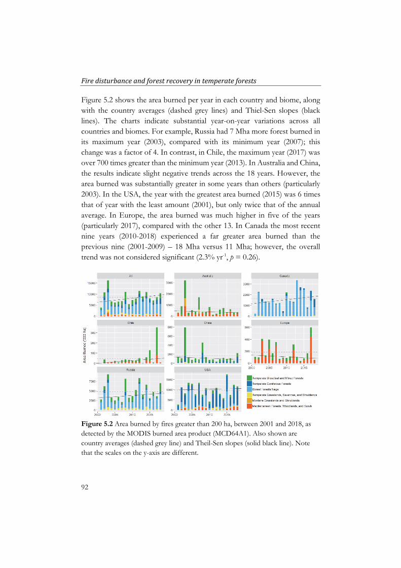
Firedisturbanceandforestrecoveryintemperateforests
92
Figure 5.2 shows the area burned per year in each country and biome, along with the country averages (dashed grey lines) and Thiel-Sen slopes (black lines). The charts indicate substantial year-on-year variations across all countries and biomes. For example, Russia had 7 Mha more forest burned in its maximum year (2003), compared with its minimum year (2007); this change was a factor of 4. In contrast, in Chile, the maximum year (2017) was over 700 times greater than the minimum year (2013). In Australia and China, the results indicate slight negative trends across the 18 years. However, the area burned was substantially greater in some years than others (particularly 2003). In the USA, the year with the greatest area burned (2015) was 6 times that of year with the least amount (2001), but only twice that of the annual average. In Europe, the area burned was much higher in five of the years (particularly 2017), compared with the other 13. In Canada the most recent nine years (2010-2018) experienced a far greater area burned than the previous nine (2001-2009) – 18 Mha versus 11 Mha; however, the overall trend was not considered significant (2.3% yr-1, p = 0.26).
Figure 5.2 Area burned by fires greater than 200 ha, between 2001 and 2018, as detected by the MODIS burned area product (MCD64A1). Also shown are country averages (dashed grey line) and Theil-Sen slopes (solid black line). Note that the scales on the y-axis are different.
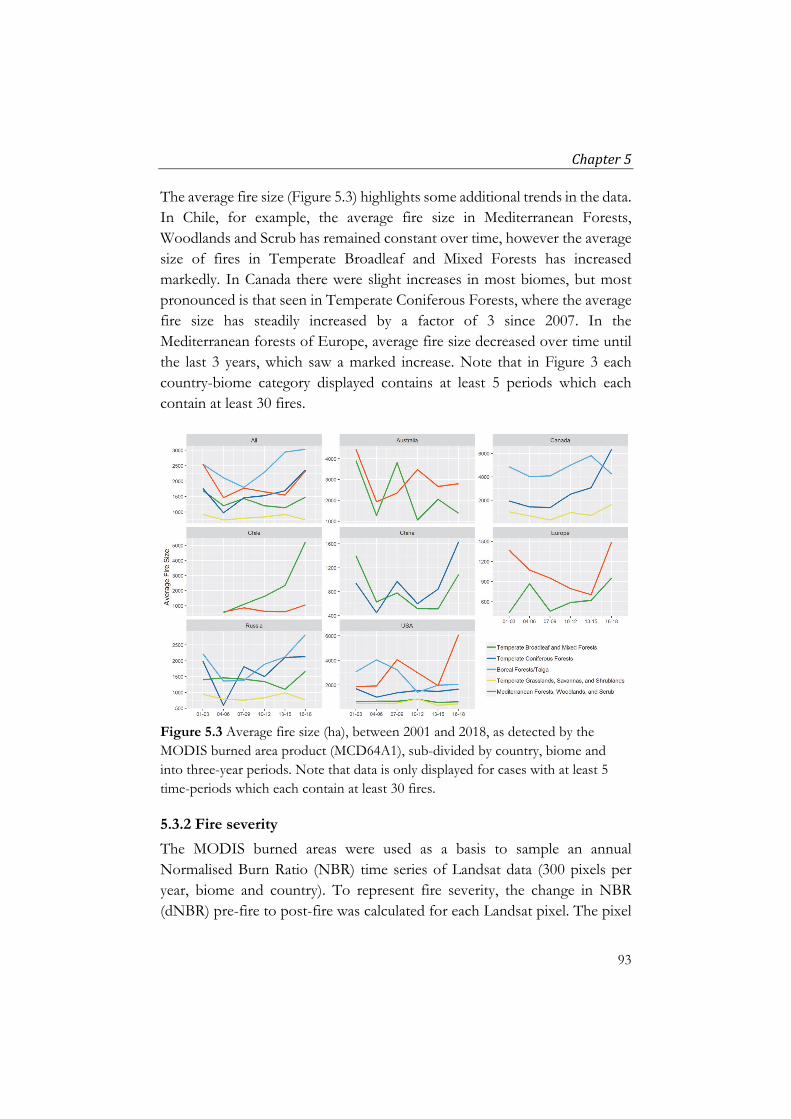
Chapter5
93
The average fire size (Figure 5.3) highlights some additional trends in the data. In Chile, for example, the average fire size in Mediterranean Forests, Woodlands and Scrub has remained constant over time, however the average size of fires in Temperate Broadleaf and Mixed Forests has increased markedly. In Canada there were slight increases in most biomes, but most pronounced is that seen in Temperate Coniferous Forests, where the average fire size has steadily increased by a factor of 3 since 2007. In the Mediterranean forests of Europe, average fire size decreased over time until the last 3 years, which saw a marked increase. Note that in Figure 3 each country-biome category displayed contains at least 5 periods which each contain at least 30 fires.
Figure 5.3 Average fire size (ha), between 2001 and 2018, as detected by the MODIS burned area product (MCD64A1), sub-divided by country, biome and into three-year periods. Note that data is only displayed for cases with at least 5 time-periods which each contain at least 30 fires.
5.3.2 Fire severity
The MODIS burned areas were used as a basis to sample an annual Normalised Burn Ratio (NBR) time series of Landsat data (300 pixels per year, biome and country). To represent fire severity, the change in NBR (dNBR) pre-fire to post-fire was calculated for each Landsat pixel. The pixel

Firedisturbanceandforestrecoveryintemperateforests
94
samples were then grouped by countries and biomes; similarities and differences are indicated by the violin plots in Figure 5.4. In Temperate Broadleaf and Mixed Forests, the fire severity distributions in most countries displayed a high amount of dispersion. Russia and the USA were exceptions, with most values grouped towards the lower end of the severity scale. In Temperate Coniferous Forests, there were also a broad range of values, especially in Canada. The severity of fires in Boreal Forests/Taiga had similar distributions in Canada and the USA (Alaska), as expected; Russia, too, was quite similar. In Temperate Grasslands, Savannas and Shrublands, the severity distributions were quite different in Australia and China, but similar in Canada and Russia. In Montane Grasslands and Shrublands, distributions were variable. In Mediterranean Forests, Woodlands and Scrub, distributions from Chile, the USA and Europe were similar, while in Australia, the distribution was clustered towards the lower end of the severity scale.
Figure 5.4 Violin plots of Landsat-based samples, showing the change in NBR (multiplied by 1000), separated by country and biome.
Median dNBR values over time are shown in Figure 4.5. These results indicate slight negative trends in fire severity in Mediterranean Forests, Woodlands and Scrub in most countries (except Chile). There are also slight negative trends in Temperate Broadleaf and Mixed Forests. In Russia there appears to be a positive trend in the Boreal Forests/Taiga biome, suggesting

Chapter5
95
that severity may be increasing. Because some of the sample sizes were low, each 3-year sample was checked to see whether it was distinct from the country-biome as a whole, by undertaking Mann-Whitney U-tests (a non-parametric equivalent of a t-test). Significantly different (α = 0.05) periods are marked in Figure 4.5 with symbols.
Figure 5.5 Median change in NBR (multiplied by 1000), divided by country, biome and into three-year periods for 2001-2018. Note that lines are shown only where samples were sufficient (> 30) and symbols mark periods where the sample was significantly different than the population (Mann-Whitney, α = 0.05).
5.3.3 Forest recovery
For each of the valid Landsat pixel samples from 2001 to 2009, the post-fire NBR time series was used to estimate the number of years for the spectral signal to return to its pre-fire level. Differences and similarities between spectral recovery times after fire are shown in the violin plots in Figure 5.6. These charts suggest many biomes respond similarly to fire across the different countries. In Temperate Broadleaf and Mixed Forests, all countries showed reasonably quick recovery times, while in Temperate Coniferous Forests and Boreal Forests/Taiga recovery tended to be longer. In Temperate Grasslands, Savannas and Shrublands, the USA and Russia showed similar distributions, while Australia, Canada and China were different. In Montane

Firedisturbanceandforestrecoveryintemperateforests
96
Grasslands and Shrublands, recovery distributions in China and Russia were similar, while the data for Australia indicated shorter post-fire recovery times. In Mediterranean Forests, Woodlands and Scrub, Australia and Europe had similar recovery distributions, while in the USA it was more dispersed; in contrast, the distribution in Chile was more tightly clustered (around 9 years).
Figure 5.6 Violin plots of Landsat-based samples, showing spectral recovery, separated by country and biome.
The median recovery times in each country-biome, divided into 3-year periods, are shown in Figure 5.7. The data suggests that, in most countries, recovery times are getting shorter. This is particularly evident in some categories: Mediterranean Forests, Woodlands and Scrub in Australia and the USA, Temperate Coniferous Forests in Canada, China, Russia and the USA, and Boreal Forests/Taiga in Canada, Russia and the USA. Again, as with the fire severity assessments, Mann-Whitney U-tests were undertaken to determine whether each 3-year period in each country-biome was significantly different (α = 0.05) than the country-biome as a whole; significant periods are marked with symbols in Figure 5.7.

Chapter5
97
Figure 5.7 Average Landsat spectral recovery, divided by country, biome and into three-year periods for 2001-2009. Note that lines are shown only where samples were sufficient (> 30) and symbols represent periods where the sample was significantly different than the population (Mann-Whitney, α = 0.05).
5.4 Discussion There is a widely held perception that, across the world, the frequency, size and severity of wildfires is increasing (Doerr and Santı, 2016). Using a combination of MODIS and Landsat satellite data, coupled with the computing power of Google Earth Engine, the above-mentioned perception was explored, by analysing fire disturbance and forest recovery trends in temperate and boreal forests across much of the world (six of the Montréal Process countries and southern Europe). The overall burned area assessment of fires greater than 200 ha, which represented approximately 90% of global temperate and boreal forests, showed an increase in burned area of 2.1% yr-1 over the 18-year period. However, the trend was not considered significant (α = 0.05) using the Mann-Kendall test for monotonic trends. Giglio et al. (2013) recently found that overall global burned areas (forest and non-forest) had slightly decreased over the past two decades. However, other studies have found increases in fire activity in some parts of the world. For example, Dennison et al. (2014) found that the occurrence of large fires (> 405 ha) in

Firedisturbanceandforestrecoveryintemperateforests
98
the western USA had increased significantly from 1984-2011. In Canada, Coops et al. (2018) found increasing trends in some ecozones and decreasing trends in others. In this assessment, significant (α = 0.05) increasing trends were found in only two cases: Temperate Coniferous Forests in Canada; and Mediterranean Forests, Woodlands and Scrub in Chile. A significant decreasing trend was also observed in Temperate Broadleaf and Mixed Forests in China. By biome, the greatest trend was found in Temperate Coniferous Forests (4.8% yr-1, p = 0.07). A slight increase (1.7% yr-1, p = 0.23) was seen in Boreal Forests/Taiga, while the other four biomes all showed slight decreasing trends.
The unpredictable nature of fire naturally leads to large year-on-year variations in area burned. Results here showed that in Australia, for example, the average area burned was approximately 1.6%, three times more than the next highest country (Russia, with 0.5%). However, in Australia, 26% of the total area burned was from one year alone (2003). Large variations were found to a greater or lesser degree in all regions (Figure 5.2). In many parts of the world it is difficult to determine to the main drivers influencing fire regimes (frequency, severity, spatial extent and pattern). Aggressive fire suppression capabilities and policies (North et al., 2015), along with strategies such as prescribed burning (Cheal, 2012) and advanced fire detection systems (Wickramasinghe et al., 2016), may be preventing large fires from eventuating, even though more humans living in the rural-urban interface often leads to more ignitions (Mann et al., 2016).
Interestingly, in Canada, the average annual burned area found here was 1.645 Mha yr-1, which is close to that of Coops et al. (2018), who arrived at a figure of 1.652 Mha yr-1, using Landsat data from 1985-2015 and including all fires in forested ecozones. That the figures are similar appears to support the assertion of Stocks et al. (2003), who found that 97% of burned area in Canada was due to fires greater than 200 ha. A similar assessment was made by North et al. (2015) in the USA, who reported that 97% of burned area was from fires greater than 120 ha. However, in the study by Coops et al. (2018) the authors calculated that only 63% of the area burned was from patches greater than 200 ha. The discrepancy could be due to the differences between the Landsat and MODIS sensors. For example, a single patch in the MODIS

Chapter5
99
data may present as several smaller patches in the Landsat data, because of the different temporal and spatial resolutions. The most recent iteration of the MODIS burned area product is substantially more accurate than previous versions (Giglio et al., 2018). Nonetheless, it still likely underestimates fires in some areas (e.g., closed canopy forests) and overestimates in others (e.g., patchy forests) (Soto-Berelov et al., 2018a). However, by consistently measuring individual points over time, overall trends will have increased accuracy, even if individual time-points suffer from systematic or random inaccuracies.
The focus in this study was on large wildfires in the temperate and boreal regions, so only MODIS burned patches greater than 200 ha were selected. While this threshold is somewhat arbitrary, it served two main purposes: (1) to filter out small burned areas, which may be due to noise or prescribed fire and (2) to create a reasonable basis for the sampling of Landsat pixels for the severity and recovery assessments. To fire ecologists, the severity (ecosystem impacts) of fires may be more important than area burned (Doerr and Santı, 2016). The results here comparing biomes across the different countries showed similar patterns in most biomes (Figure 5.4). It should be noted that dNBR is not an ideal measure of fire severity (Roy et al., 2006) and is typically used in conjunction with field data to determine severity classifications (e.g., high, medium, low) (Key and Benson, 2006). The wide range of values observed in many countries and biomes could equally be due to the pre-fire vegetation conditions as the post-fire conditions. Nonetheless, by measuring the dNBR metric over time, in the same location and forest type, trends may emerge, which could indicate that forest resilience is being threatened. To date, few studies have examined this. In a recent review of global wildfire trends, Doerr and Santı (2016) list a couple of studies in the USA, which did not find any broad trends. Likewise, the fire severity results here did not find any widespread patterns. Admittedly, 18 years is not a long time-period for global change in fire severity. However, a positive trend in dNBR was observed in the Russian taiga and there were some slight negative trends in Mediterranean type forests elsewhere. The perception that fire intensity is increasing may therefore be more attributable to increased human populations and media coverage, rather than systemic ecological changes. Historical accounts of the 1939 bushfires in Australia, for example, indicate

Firedisturbanceandforestrecoveryintemperateforests
100
that those fires were as severe as today’s fires (Stretton, 1939). Nonetheless, the method presented here may reveal significant patterns in future and it is suggested that the dNBR metric deserves continual monitoring.
It is largely accepted that climate change will alter fire regimes, and the capacity of forests to recover, worldwide (Enright et al., 2015). However, the effects are likely to be complex. For example, warmer weather may extend growing seasons in some areas, while restricting growth in others. Increased droughts may reduce fuel loads, while simultaneously making existing fuels more flammable (MIG and NFISC, 2013). Some have suggested that higher carbon dioxide levels can increase growth (CO2 fertilization); however, other factors, such as water availability, are thought to exert far more influence (Appenzeller, 2015). Forest recovery results in this study showed similarities between the same biomes in different countries. Temperate Broadleaf and Mixed forests, which occur in all six countries and in Europe, tended to return quickly to their pre-fire spectral values, ranging from an average of 8 years (Australia and China) to 12 years (Canada). In contrast, Temperate Coniferous Forests took between 14 years (China) to 20 years (Canada and USA) to recover, but with more variation, as shown by the dispersed violin plots (Figure 5.6). In the boreal forests of Canada and Alaska, and the taiga in Russia, the average recovery times were quite similar (16, 15 and 17 years respectively). That the same biomes in different countries are responding similarly is perhaps unsurprising, but it is also reassuring in that the method appears transferable across a wide range of environments.
Several regions showed signs of accelerating recovery. Although 18 years is a short time-period, especially because data is needed for several years after each fire (to measure recovery trajectories), results indicated decreasing recovery times, particularly in boreal and temperate coniferous forests. This may be partly explained by the reliance on a linear model to estimate recovery, as a regression line fitted through the years directly following a fire may fail to adequately estimate a slower rate of recovery beyond the time series. Nonetheless, a linear model of spectral recovery is a pragmatic approach that has proved capable in other studies (Kennedy et al., 2012; White et al., 2018). In addition, the manual evaluation of 600 pixels indicated that the method produced acceptable approximations in 92% of cases. It is worth noting that,

Chapter5
101
globally, the five warmest years on record have all occurred since 2010 (www.climatecentral.org), which may have lengthened the growing season in certain regions, accelerating forest recovery. However, the results here may also reflect changes in vegetation type. In the boreal forests of Canada, studies have found that, recently, following wildfires, black spruce has been replaced by aspen and birch; to a satellite these deciduous trees appear brighter (Appenzeller, 2015). Continuing to monitor forest recovery over the coming years will help affirm or discredit the findings of this study.
5.5 Conclusions Forest disturbance and subsequent regeneration is a natural and essential ecological process, but recent anthropogenic drivers may be exerting undue influences, and thereby threatening the resilience of forests. Consequently, monitoring and reporting on these measures is recognised through international frameworks such as the Montréal Process. In this chapter, a straightforward and methodical approach was used to estimate large-area trends in fire disturbance and forest recovery with freely available satellite data in a cloud computing environment. The 18-year analysis of boreal and temperate forests illuminated possible trends in area burned in certain biomes and indicated that forest recovery was accelerating in some cases. The approach outlined here can be used to improve reporting on key forest indicators, which in turn can lead to more informed management strategies and a greater understanding of the essential and inevitable role that fire plays in many ecosystems.

Firedisturbanceandforestrecoveryintemperateforests
102

103
Chapter 6: Synthesis This chapter provides an overview of the key results from each of the core chapters, linking them to the research objectives as stated in the introduction. The research is then discussed in a broader context, including future directions and opportunities for the science and technologies.

Synthesis
104
6.1 Summary of results This research had four primary objectives, each of which was addressed in a core chapter. A summary of the main results is provided below. The objectives are re-stated as they are addressed.
Chapter 2 addressed research objective 1, which was to:
Assess the potential of a number of Landsat-based spectral indices in their ability to detect fire disturbance and characterise subsequent forest recovery in southeast Australian forests
In this section of research, a number of tests were undertaken to evaluate the merits of 8 Landsat-derived spectral indices in their ability to detect wildfire disturbance and characterise forest recovery in southeast Australian forests. Although there is substantial literature assessing and comparing various Landsat indices, studies in the unique forests of southeast Australia are limited. In addition, the methods presented in this chapter introduced several novelties.
The primary method employed to determine an index’s suitability was to consider disturbed pixels as a group and calculate the average change pre-fire to post-fire, along with the standard deviation, as a measure of dispersion. To compare indices, values were converted to a standardised scale, using Glass’s delta. The results showed that greenness indices like NDVI and TCA on average, changed by a large amount directly following a fire, however, returned to pre-fire conditions within a short period of time. In contrast wetness indices, using the SWIR bands, tended to take longer to recover their pre-fire values, which agrees with studies conducted elsewhere (Pickell et al., 2016; Schroeder et al., 2011).
There were other findings from chapter 2 that warrant mentioning. In contrast to studies elsewhere (e.g., Frazier et al., 2015), TCW was not found to be optimal for detecting forest disturbances in the study area. The rarely used NBR2 index (which contrasts the two SWIR bands) indicated longer spectral recovery times; therefore, it may be more sensitive to subtleties of forest recovery missed by the other indices. And the analysis of texture-based

Chapter6
105
indices indicated that, in this regard, it was the greenness indices, rather than the wetness indices that took longer to return to their pre-fire levels. Ultimately NBR2 and texture indices were not used further in this body of work; however, future opportunities remain to include these outputs in broader modelling applications. Texture, for example, could contribute to models based on objects or patches, rather than individual pixels.
The conclusion from chapter 2 was that NBR was the most reliable index to use within an annual time series for southeast Australian sclerophyll forests, if only one index was to be adopted, as it was adept at both capturing fire disturbance and characterising subsequent forest recovery. However, the results from chapter 2 re-enforced the fact that different indices capture different elements of forest disturbance. Consequently, it was conjectured that an ensemble of indices would lead to more accurate forest disturbance maps.
In chapter 3, this hypothesis was tested by undertaking a study comparing two change detection algorithms (LandTrendr and strucchange), each with three indices (NDVI, NBR and TCW), in their ability to detect disturbances in southeast Australian forests. Several ensembles were then created, using a range of variables, in conjunction with human interpreted reference data, to ‘predict’ disturbance, using both simple aggregation rules and the Random Forests algorithm, to determine class assignment. Chapter 3 addressed research objective 2, which was to:
Explore the benefits of using an ensemble of spectral indices, in conjunction with human interpreted reference data and machine learning, to produce forest disturbance maps
Results showed that the most accurate individual algorithm/index combination was LandTrendr and NBR, with omission and commission errors of 37% and 15% respectively, and an overall error of 21%. The least accurate algorithm/index was strucchange with TCW, which had omission, commission and overall errors of 47%, 34% and 38% respectively. It is worth noting that LandTrendr outperformed strucchange with all indices.

Synthesis
106
The simple ensembles were formed by aggregating individual change detection algorithm outputs. The results here showed that as rules were tightened (i.e., a greater number of change detection outputs were needed) the commission errors decreased substantially, but at the expense of increases in omission errors. The 4 out of 6 ensemble, for example, only had a commission error of 3%, but had an omission error of 48%. These results highlight that outputs can vary substantially, depending on the algorithm and index used; a finding which aligns with those from other studies (Cohen et al., 2017a).
The simple aggregation technique may be effective if the specific aims of the study call for a preference towards low errors of commission. Technically, this approach, and change detection algorithms more generally, do not need reference data. However, without reference data for validation, the accuracy is unknown. In contrast, machine learning approaches using algorithms like Random Forests, need reference data for training purposes. The most accurate ensemble, a Random Forests model that included the six change detection algorithm outputs, along with three change rasters (dNBR, dNDVI and dTCW), had omission and commission errors of 14% and 4% respectively, with an overall error of 7%.
One of the findings from chapter 3 was that ‘priming’ the training data with confusing cases resulted in far fewer commission errors, at the expense of omission errors, which slightly increased. The confusing cases were generated by using the commission errors (i.e., incorrectly detected disturbances) from the change detection algorithms. Healey et al. (2018) also used the technique of priming (or ‘skewing’) the dataset towards confusing cases, but did not formally evaluate the effects. This finding led to the conclusion that traditional change detection algorithms (such as LandTrendr) could potentially be used on a subset of pixels only, as a means of priming a classifier (e.g., Random Forests) with confusing cases.
Acceptable results were found using a Random Forests ensemble with only three predictor variables (dNBR, dNDVI, and dTCW) and the primed training data (overall error 11.4%). By including a range of other Landsat time series derived metrics, such as overall means and standard deviations, along

Chapter6
107
with 2-year changes (referred to as the ‘extended model’ in chapter 3), the overall error decreased to 8.5%. This model was then used to predict the presence or absence of forest disturbance for each year in the time series (1989-2017) for the state of Victoria, Australia (Figure 6.3).
The disturbance maps generated in chapter 3 were used in a number of other applications (see inset box on the following page), including the basis for the segmented NBR time series used in chapter 4.
The aim of chapter 4 was to test the hypothesis that a higher fire disturbance results in a longer recovery time, as measured spectrally with Landsat time series. The relationship (or statistical association) between the magnitude of fire disturbance and forest recovery length was examined at a range of spatial scales. Chapter 4 addressed research objective 3, which was to:
Examine the relationship between spectral disturbance magnitude and recovery length, to determine: a) Whether a statistical association exists, and how well it can be
characterised using Landsat time series b) How the association varies across different forest types
In chapter 4, forest disturbance and recovery maps were first created across the state of Victoria, Australia, using 13 major fire events to inform the study areas. A total of 2.3 million ha of burned forest was analysed in this section of research. Spectral disturbance was based on the post-fire change in NBR (dNBR), while the spectral recovery length was calculated by taking the post-fire segment of each pixel’s temporal trajectory and determining the number of years for this line to reach the pre-fire condition. To explore the relationship between disturbance magnitude and recovery length, as measured spectrally, Pearson correlations were computed across different spatial scales. First, an overall correlation, using all pixels in the study area (~25 million) was calculated, which gave a result of -0.01. Following this the data were subdivided according to biogeographic regions. Correlations within bioregions were predominately positive (i.e., a larger disturbance magnitude equalled a longer recovery length), however most correlations were weak. The strongest was 0.34, in the state’s most arid region (Murray Darling Depression in northwest Victoria).

Synthesis
108
Other uses for yearly disturbance maps
Classification by disturbance type The results of chapter 3 were used in a secondary classification of disturbances by type – fire, logging and drought. The classified maps were then used to construct a video of disturbance over time in Victorian forests, to easily disseminate the information to non-experts. (To view the video, see https://youtu.be/Frplhhl8P_k).
Seamless gap-free mosaics The results were also used to create seamless, gap free synthetic Landsat mosaics for each year from 1988 to 2017, by fitting a piece-wise linear model through each of the six Landsat optical bands (Hislop et al., 2018). In this process, data gaps and other radiometric anomalies were removed. The resultant mosaics have several potential applications, particularly in spatial modelling. As an example, Nguyen et al. (2019) used the mosaics to estimate above ground biomass for each year in the time series. Figure 6.1 shows derived biomass dynamics (loss and gain) resulting from forest disturbance events between 1988 and 2017.
Figure 6.1 Biomass dynamics (loss and gain) following disturbance in Victoria, Australia. Reprinted with permission from Nguyen et al. (2019)

Chapter6
109
It was conjectured that there were confounding factors influencing both the disturbance magnitude (dNBR) and the recovery length. To isolate the disturbance-recovery association from other influences, such as soil type, elevation, climate, etc., a novel patch-based solution was used. First, a 600 m × 600 m grid was defined over the entire burned area. Then within each grid square, or ‘patch’, the correlation between disturbance magnitude and recovery length was calculated. These results clearly revealed spatial patterns, indicating that in some areas there was a strong positive relationship, while in others the opposite behaviour was apparent (Figure 4.5).
The patch-level results were also subdivided by bioregion, which showed statistically significant differences between bioregions (Figure 4.6). To test the method at a finer spatial scale, a case study into one bioregion, the South Eastern Highlands, was undertaken. The five most dominant vegetation divisions (Cheal, 2010) were used to further subdivide the patches. These results also showed statistically significant differences between most vegetation divisions (Figure 4.7).
Chapter 4 demonstrated a novel approach to exploring Landsat time series in greater detail. That different vegetation types respond differently to fire disturbance is perhaps not surprising, but by using Landsat data, landscape-wide assessments are possible, which can support better land management strategies.
While chapter 4 narrowed the focus and perhaps tested the limits of Landsat in its ability to detect fine scale ecological processes, chapter 5 ventured in the opposite direction, taking the lessons learned from chapters 2, 3 and 4 and applying them to an extremely large-area study, investigating temperate and boreal forests across the world.
Chapter 5 addressed research objective 4, which was to:
Investigate fire disturbance and forest recovery in boreal and temperate forests worldwide, using the MODIS and Landsat image archives, to: a) Explore trends in burned area, fire severity (change in NBR) and
forest recovery lengths (as measured spectrally)

Synthesis
110
b) Establish similarities and differences between similar forest types in different countries
c) Determine the transferability and scalability of methods developed in the previous objectives.
Although forests have evolved in parallel with fire, there is a concern that changes to fire regimes (frequency, severity, spatial extent and pattern) may threaten the resilience of forests (Enright et al., 2015; Jolly et al., 2015; Millar and Stephenson, 2015). In chapter 5, large area trends in fire disturbance, using both MODIS and Landsat satellite data within Google Earth Engine, were explored, for the period of 2001 to 2018. Results were divided in a jurisdictional sense (by country) and an ecological sense (by WWF biome).
The area estimates were based on the MODIS burned area monthly product (MCD64A1), filtered to fires greater than 200 ha in size (based on burned area patches). A total of 154 million ha of forest was burned across the study area (1.98 billion ha) between 2001 and 2018 (an average of 8.5 million ha per year). Three significant trends (α = 0.05) in area burned were identified: Temperate Coniferous Forests in Canada (slope: 5.1% yr-1, p = 0.04), Mediterranean Forests, Woodlands, and Scrub in Chile (7.5% yr-1, p = 0.03) and Temperate Broadleaf and Mixed Forests in China (-2.5% yr-1, p = 0.03). Over the entire study area, the slope was 2.1% yr-1 (p = 0.17).
The MODIS burned areas were used as a basis for a stratified sampling of Landsat pixels. In a process similar to that used in chapter 4, NBR pixel trajectories were analysed to extract ‘fire severity’ – defined as the post-fire change in NBR (dNBR) – and ‘forest recovery’ – defined as the number of years for the NBR pixel trajectory to return to its pre-fire level. Figure 6.2 shows the calculated spectral recovery length for a sample of Landsat pixels across North America and Australia. This figure highlights visually that spectral recovery is dependent on location. Pixels were grouped by country and biome to explore similarities and differences, and trends over time. Results showed that corresponding biomes in different countries responded to fire similarly, as indicated by violin plots (Figures 5.4 and 5.6).

Chapter6
111
Figure 6.2 Years to recover spectrally, based on a sample of Landsat pixels across North America and Australia
Widespread changes in dNBR over the 18 years were not observed. However, there were a few trends which may in time prove significant. Most notably, in the Russian taiga, where results suggested that dNBR was increasing over time. The investigation into recovery length suggested that spectral recovery was accelerating in many regions, across the 9 years analysed. Although it is a short period of time, these results may reflect changes to underlying ecological processes. In the boreal forests of Canada, for example, it has recently been reported that, following fire, the endemic black spruce is often being replaced by aspen and birch, which may appear brighter (particularly in the near infrared) to satellites (Appenzeller, 2015).
The 18-year time-scale used in chapter 5 is perhaps not long enough to form robust conclusions; however, it was restricted by the availability of the MODIS satellite data, which does not exist prior to 2000. There are potential opportunities to extend the research back to at least the late 80s in many regions, using only Landsat data. In addition, a repeat of the study in 5 or 10 years’ time may reveal a greater number of significant trends.
6.2 Broader implications of research Forests have evolved in the presence of disturbances such as fire, drought, storms, diseases and pests. Over time, disturbance regimes and evolutionary

Synthesis
112
processes have led to a certain level of resilience being built into the system. However, recent unprecedented population growth and associated anthropogenic pressures have altered forests outside of the ranges that they are accustomed to, thus threatening overall ecosystem health (Trumbore et al., 2015). The maintenance of forest ‘health and vitality’ is therefore a key element of international forest reporting frameworks, such as the Montréal Process (Montréal Process, 2009), and seen as vital to achieving the United Nations Sustainable Development Goals (FAO, 2018). Accurate monitoring of forest disturbance across all spatial scales is fundamental to the maintenance of forests and can support better land management strategies and policies.
Funded under a broader forest monitoring project, this research, along with that led by colleagues (Nguyen et al., 2018b, 2018a; Soto-Berelov et al., 2017), investigated forest disturbance and recovery in southeast Australian sclerophyll forests. Until recently, landscape-wide studies in southeast Australia were lacking, so the research provides a significant contribution to forest monitoring and reporting in the region.
More broadly, the research presented a range of new and novel approaches to characterise forest disturbance and recovery using satellite time series, particularly Landsat. Chapter 2 presented exploratory analysis techniques for testing the sensitivity of spectral indices to forest disturbance and recovery. Chapter 3 demonstrated that ensemble approaches produce more accurate maps of forest disturbance and argued that traditional change detection algorithms could be applied to a subset of pixels only. Chapter 4 used the results of Chapter 3 to segment the Landsat time series data, to produce maps of disturbance magnitude and spectral recovery across large fire events in Victoria, Australia. The research then shifted into an ecological realm to investigate whether there was a statistical association between the magnitude of disturbance (as a proxy for fire severity) and the time that a forest takes to recover spectrally. A novel patch-based technique was presented, which helped to isolate the disturbance-recovery relationship from confounding factors such as climate, elevation, soils and vegetation type. In chapter 5, the applications developed in the previous chapters were employed over a much

Chapter6
113
larger area, to investigate trends in fire disturbance and forest recovery in temperate and boreal forests worldwide.
Trends in fire area, fire severity and forest recovery length highlight areas where fire regimes may be changing. Significant, or substantial, trends may indicate underlying ecological changes, and thus warrant further attention from land managers and policy makers. On the other hand, in areas where no trends are evident, but a perception exists that fire activity is increasing, evidence-based studies, like those presented here, can help to dispel myths. The methods and results presented in this thesis demonstrate that Earth observation satellites, offering wall-to-wall coverage at regular time steps, add enormous value to the monitoring and reporting of key forest indicators.
6.3 Future directions and opportunities There is a growing realisation that humanity needs to act quickly to limit the worst impacts of global warming and other environmental concerns, such as biodiversity loss. Global action not only requires international collaboration; it also needs mechanisms in place to monitor changes. While policy frameworks provide the necessary direction, they do not in themselves offer the means for effective monitoring. Earth observation satellites, from their unique perspective, are ideally suited to monitor the Earth’s land, oceans and atmosphere at the large-area scale. It is perhaps serendipitous that the capabilities of Earth observation satellites have developed in unison with advancements in communications, computer processing and data storage. In addition, a shift towards free and open access to data, and knowledge sharing, is enabling global monitoring via satellites to be undertaken in unprecedented ways (Figure 6.3).
This convergence of multiple technologies, coupled with a culture of openness, means that opportunities are vast indeed. The free and open access policies, perhaps kick-started in 2008 with the opening of the Landsat archive (Wulder et al., 2012), have broken down barriers to accessibility, while platforms such as Google Earth Engine (Gorelick et al., 2017) are enabling users to rapidly process vast quantities of data and perform planetary-scale geospatial analysis.

Synthesis
114
Figure 6.3 Convergence of technologies, leading to advanced environmental monitoring opportunities
A few of the more recent and planned Earth observation satellites, which are relevant to large-area forest monitoring, will be discussed below, along with some of the nascent methods that will help improve outputs and inform sustainable management strategies. Avenues of future research opportunities are also mentioned.
The Sentinel satellites, developed and operated by the European Space Agency (ESA) and the European Commission (EC) through the Copernicus initiative, are a series of satellites designed to provide timely and accurate information to improve environmental management and civil security (Drusch et al., 2012). The Sentinel 2A and 2B satellites are a natural companion to Landsat. Together, the two satellites offer a 5 day re-visit time,

Chapter6
115
13 bands in the visible, near infrared and shortwave infrared wavelengths, spatial resolutions from 10 m to 60 m (depending on the spectral band) and a 295 m field of view (Gascon et al., 2017).
Due to the similarities between Landsat 8 and Sentinel 2, opportunities exist to use the data in tandem, allowing for more frequent cloud-free observations. In a recent paper Li and Roy (2017) calculated that the combined ‘virtual constellation’ offered a global median revisit time of 2.9 days. However, the use of these data in time series analysis requires cross-sensor calibration. While some research has addressed this (Ganguly et al., 2017; Zhang et al., 2018), further work is required.
One of the advantages of the Sentinel 2 sensor over Landsat 8, is the inclusion of red-edge bands (the portion of the electromagnetic spectrum between the red and near-infrared wavelengths). Previous studies using RapidEye imagery have highlighted the usefulness of the red-edge in detecting plant stress (Ager et al., 2011). In a recent study, Abdullah et al. (2018) reported that Sentinel 2, using red-edge spectral indices, was more accurate than Landsat 8 in mapping bark beetle disturbance in European spruce at the early stage of attack. The potential of Sentinel 2 for forest monitoring (given it has higher spatial, spectral and temporal resolutions than Landsat) is yet to be fully explored. It is envisaged that Sentinel 2 will prove useful in capturing subtle and low severity forest disturbances, such as insect defoliation and selective logging, along with providing higher spatial resolution maps of forest cover.
Although Sentinel 2 has more bands than Landsat, it is still a multispectral instrument. Hyperspectral satellite technology, on the other hand, is still in its infancy. NASA’s Hyperion imaging spectrometer, launched in 2000, demonstrated that spaceborne spectroscopy was possible. Hyperion collected data across 242 narrow bands in the visible, near infrared and shortwave infrared regions (Pearlman et al., 2003). The results of the Hyperion mission, along with the recently deployed DLR Earth Sensing Imaging Spectrometer (DESIS) onboard the International Space Station (ISS), serve to inform future missions, such as Germany’s Environmental Mapping and Analysis Program (EnMAP). EnMAP will enable geochemical, biochemical and
Synthesis
116
biophysical parameters to be measured in fine detail, broadening our understanding of the Earth’s ecosystems (www.enmap.org).
Wulder et al. (2015) extended the concept of a virtual constellation to include sensors which are principally incompatible (e.g., passive sensors and active sensors) but can be integrated to achieve a specific monitoring goal. Virtual constellations may help overcome the limitations of single sensors (e.g., by providing more cloud-free images), however, cross-sensor integration and harmonization remains challenging. Machine learning via non-parametric classifiers such as Random Forests offers a means for integrating otherwise incompatible datasets; ideally, each dataset provides complimentary information.
The recent drive to curtail CO2 emissions to limit global warming has focussed attention on the role of forests as carbon sources and sinks. Consequently, modelling biomass dynamics across large areas has been the focus of a number of recent studies (Kennedy et al., 2018a; Matasci et al., 2018; Nguyen et al., 2018a). Above ground biomass is more closely aligned with forest structure, which can be estimated with field measurements or lidar, but is less easily determined via passive remote sensing. However, field data and lidar are not generally available over large areas or consistently through time. Combining field data and/or lidar with satellite data, through machine learning imputation approaches, can provide wall-to-wall estimates of forest biomass across large areas (Nguyen et al., 2018a). This may be particularly useful in countries where established forest monitoring programs are lacking.
Spaceborne lidar has the potential to provide more accurate measurements of forest structure. The recent deployment of the Global Ecosystem Dynamics Investigation (GEDI) instrument onboard the ISS will provide lidar samples with a 25 m footprint every 60 m in the along-track direction and 600 m across-track. GEDI will provide ‘globally representative measurements of vertical structure in the world’s temperate and tropical forests’ (https://gedi.umd.edu). However, GEDI does not offer wall-to-wall coverage and is limited by the orbit of the ISS, which does not extend into the northern boreal forests (Wulder et al., 2015). Thus, the use of GEDI data

Chapter6
117
will inevitably require upscaling using wall-to-wall Earth observation and machine learning approaches.
While spaceborne lidar is in its infancy, spaceborne radar is arguably further advanced. The Sentinel 1 satellite carries a C-band synthetic aperture radar (SAR), which can penetrate clouds, making it particularly useful in cloudy regions. An advantage of the C-band SAR is the continuity it offers; a number of satellites (Envisat ASAR, ERS, and Radarsat) have acquired compatible C-band data for over 20 years (Wulder et al., 2015). However, C-band radar is less sensitive to forest structure than that at longer wavelengths. Nonetheless, Haywood et al. (2018) recently found that integrating Sentinel 1 data into a model estimating forest biomass improved results. In 2020, ESA is planning to launch a satellite dedicated to measuring forest biomass, which will have a P-band SAR, a wavelength more capable of penetrating the forest canopy (Wulder et al., 2015).
6.4 Final remarks The future of Earth observation looks bright across much of the electromagnetic spectrum. However, to capitalise on these new technologies, skills and knowledge beyond traditional fields of geospatial and remote sensing are required. The enormous amounts of data, much of which is freely available, is both advantageous and cumbersome. To make use of such data, computer science and machine learning skills are increasingly required. In addition, a strong grasp of statistics ensures that models are correctly constructed and evaluated, and assumptions and accuracies are transparent. Perhaps most importantly, a shared understanding between the remote sensing and ecological communities, on what can and should be measured from space, will lead to outcomes that translate into achievable management strategies and inform policy directions.

Synthesis
118

119
Bibliography Abdullah, H., Skidmore, A.K., Darvishzadeh, R., Heurich, M., 2018. Sentinel-2 accurately
maps green-attack stage of European spruce bark beetle ( Ips typographus , L.) compared with Landsat-8. Remote Sens. Ecol. Conserv. 1–21. https://doi.org/10.1002/rse2.93
Adams, M.A., 2013. Mega-fires, tipping points and ecosystem services: Managing forests and woodlands in an uncertain future. For. Ecol. Manage. 294, 250–261. https://doi.org/10.1016/j.foreco.2012.11.039
Ager, A.A., Litvak, M.E., Eitel, J.U.H., Stoscheck, L., Vierling, L.A., Long, D.S., Schulthess, U., Krofcheck, D.J., 2011. Broadband, red-edge information from satellites improves early stress detection in a New Mexico conifer woodland. Remote Sens. Environ. 115, 3640–3646. https://doi.org/10.1016/j.rse.2011.09.002
Appenzeller, T., 2015. The New North. Science (80-. ). 349, 806–809. https://doi.org/10.1126/science.349.6250.806
Attiwill, P.M., Adams, M.A., 2013. Mega-fires, inquiries and politics in the eucalypt forests of Victoria, south-eastern Australia. For. Ecol. Manage. 294, 45–53. https://doi.org/10.1016/j.foreco.2012.09.015
Australian Government, 2017. Australia’s bioregions (IBRA) [WWW Document]. Dep. Environ. Energy. URL http://www.environment.gov.au/land/nrs/science/ibra (accessed 8.4.18).
Bassett, O.D., Prior, L.D., Slijkerman, C.M., Jamieson, D., Bowman, D.M.J.S., 2015. Aerial sowing stopped the loss of alpine ash (Eucalyptus delegatensis) forests burnt by three short-interval fires in the Alpine National Park, Victoria, Australia. For. Ecol. Manage. 342, 39–48. https://doi.org/10.1016/j.foreco.2015.01.008
Becker, L.A., 2000. Effect Size ( ES ) [WWW Document]. URL http://www.bwgriffin.com/gsu/courses/edur9131/content/EffectSizeBecker.pdf accessed 5/8/2017 (accessed 8.5.17).
Bennett, L.T., Bruce, M.J., Machunter, J., Kohout, M., Tanase, M.A., Aponte, C., 2016. Forest Ecology and Management Mortality and recruitment of fire-tolerant eucalypts as influenced by wildfire severity and recent prescribed fire. For. Ecol. Manage. 380, 107–117. https://doi.org/10.1016/j.foreco.2016.08.047
Bolton, D.K., Coops, N.C., Wulder, M.A., 2015. Characterizing residual structure and forest recovery following high-severity fire in the western boreal of Canada using Landsat time-series and airborne lidar data. Remote Sens. Environ. 163, 48–60. https://doi.org/10.1016/j.rse.2015.03.004
Bond, W.J., Keeley, J.E., 2005. Fire as a global “herbivore”: The ecology and evolution of flammable ecosystems. Trends Ecol. Evol. 20, 387–394.

Bibliography
120
https://doi.org/10.1016/j.tree.2005.04.025
Bowman, D.M.J.S., Balch, J.K., Artaxo, P., Bond, W.J., Carlson, J.M., Cochrane, M.A., Antonio, C.M.D., Defries, R.S., Doyle, J.C., Harrison, S.P., Johnston, F.H., Keeley, J.E., Krawchuk, M.A., 2010. Fire in the Earth System. Science (80-. ). 481, 481–485. https://doi.org/10.1126/science.1163886
Breiman, L., 2001. Random Forests, in: Machine Learning. pp. 5–32.
Cheal, D., 2012. A biological basis for planned burning. Proc. R. Soc. Victoria 124, 7–19. https://doi.org/10.1071/RS12007
Cheal, D., 2010. Growth stages and tolerable fire intervals for Victoria’s native vegetation data sets. Fire and Adaptive Management Report No. 84. East Melbourne, Victoria, Australia.
Cocke, A.E., Fulé, P.Z., Crouse, J.E., A, A.E.C., A, P.Z.F., B, J.E.C., 2005. Comparison of burn severity assessments using Differenced Normalized Burn Ratio and ground data. Int. J. Wildl. Fire 14, 189. https://doi.org/10.1071/WF04010
Cohen, W., Yang, Z., Stehman, S. V., Schroeder, T.A., Bell, D.M., Masek, J.G., Huang, C., Meigs, G.W., 2016. Forest disturbance across the conterminous United States from 1985-2012: The emerging dominance of forest decline. For. Ecol. Manage. 360, 242–252. https://doi.org/10.1016/j.foreco.2015.10.042
Cohen, W.B., Goward, S.N., 2004. Landsat’s Role in Ecological Applications of Remote Sensing. Bioscience 54, 535–545.
Cohen, W.B., Healey, S.P., Yang, Z., Stehman, S. V., Brewer, C.K., Brooks, E.B., Gorelick, N., Huang, C., Hughes, M.J., Kennedy, R.E., Loveland, T.R., Moisen, G.G., Schroeder, T.A., Vogelmann, J.E., Woodcock, C.E., Yang, L., Zhu, Z., 2017a. How Similar Are Forest Disturbance Maps Derived from Different Landsat Time Series Algorithms? Forests 8, 1–19. https://doi.org/10.3390/f8040098
Cohen, W.B., Yang, Z., Healey, S.P., Kennedy, R.E., Gorelick, N., 2017b. A LandTrendr Multispectral Ensemble for Forest Disturbance Detection. Remote Sens. Environ. 205, 11–13. https://doi.org/10.1016/j.rse.2017.11.015
Cohen, W.B., Yang, Z., Kennedy, R.E., 2010. Detecting trends in forest disturbance and recovery using yearly Landsat time series: 2. TimeSync - Tools for calibration and validation. Remote Sens. Environ. 114, 2911–2924. https://doi.org/10.1016/j.rse.2010.07.010
Coops, N.C., Hermosilla, T., Wulder, M.A., White, J.C., Bolton, D.K., 2018. A thirty year, fine-scale, characterization of area burned in Canadian forests shows evidence of regionally increasing trends in the last decade. PLoS One 13, 1–19. https://doi.org/10.1371/journal.pone.0197218

Bibliography
121
Crist, E.P., 1985. SHORT COMMUNICATION A TM Tasseled Cap Equivalent Transformation for Reflectance Factor Data. Remote Sens. Environ. 17, 301–306. https://doi.org/10.1016/0034-4257(85)90102-6
Crist, E.P., Cicone, R.C., 1984. A Physically-Based Transformation of Thematic Mapper Data-The TM Tasseled Cap. IEEE Trans. Geosci. Remote Sens. GE-22, 256–263. https://doi.org/10.1109/TGRS.1984.350619
Dennison, P.E., Brewer, S.C., Arnold, J.D., Moritz, M.A., 2014. Large wildfire trends in the western United States, 1984–2011. Geophys. Res. Lett. 2928–2933. https://doi.org/10.1002/2014GL059576.Received
Department of Environment and Primary Industries, 2013. Victoria’s State of the Forests Report 2013.
Department of Environment Land Water and Planning, 2017. Fire History Records of Fires Primarily on Public Land [WWW Document]. URL www.data.vic.gov.au (accessed 8.10.17).
DeVries, B., Decuyper, M., Verbesselt, J., Zeileis, A., Herold, M., Joseph, S., 2015. Tracking disturbance-regrowth dynamics in tropical forests using structural change detection and Landsat time series. Remote Sens. Environ. 169, 320–334. https://doi.org/10.1016/j.rse.2015.08.020
Devries, B., Verbesselt, J., Kooistra, L., Herold, M., 2015. Robust monitoring of small-scale forest disturbances in a tropical montane forest using Landsat time series. Remote Sens. Environ. 161, 107–121. https://doi.org/10.1016/j.rse.2015.02.012
Doerr, S.H., Santı, C., 2016. Global trends in wildfire and its impacts: perceptions versus realities in a changing world. Philos. Trans. B. https://doi.org/10.1098/rstb.2015.0345
Drusch, M., Bello, U. Del, Carlier, S., Colin, O., Fernandez, V., Gascon, F., Hoersch, B., Isola, C., Laberinti, P., Martimort, P., Meygret, A., Spoto, F., Sy, O., Marchese, F., Bargellini, P., 2012. Sentinel-2: ESA’s Optical High-Resolution Mission for GMES Operational Services. Remote Sens. Environ. 120, 25–36. https://doi.org/10.1016/j.rse.2011.11.026
Dube, T., Mutanga, O., 2015. Investigating the robustness of the new Landsat-8 Operational Land Imager derived texture metrics in estimating plantation forest aboveground biomass in resource constrained areas. ISPRS J. Photogramm. Remote Sens. 108, 12–32. https://doi.org/10.1016/j.isprsjprs.2015.06.002
Dutrieux, L.P., Jakovac, C., Latifah, S.H., Kooistra, L., 2016. Reconstructing land use history from Landsat. Int. J. Appl. Earth Obs. Geoinf. https://doi.org/10.1016/j.jag.2015.11.018
Dutrieux, L.P., Verbesselt, J., Kooistra, L., Herold, M., 2015. Monitoring forest cover loss

Bibliography
122
using multiple data streams, a case study of a tropical dry forest in Bolivia. ISPRS J. Photogramm. Remote Sens. 107, 112–125. https://doi.org/10.1016/j.isprsjprs.2015.03.015
Eidenshink, J., Schwind, B., Brewer, K., Zhu, Z., Quayle, B., Howard, S., 2007. A project for monitoring trends in burn severity. Fire Ecol. 3, 3–21. https://doi.org/10.4996/fireecology.0301003
Eklundh, L., Jönsson, P., 2015. TIMESAT: A Software Package for Time-Series Processing and Assessment of Vegetation Dynamics, in: Remote Sensing Time Series. pp. 141–157. https://doi.org/10.1007/978-3-319-15967-6
Enright, N.J., Fontaine, J.B., Bowman, D.M.J.S., Bradstock, R.A., Williams, R.J., 2015. Interval squeeze: Altered fire regimes and demographic responses interact to threaten woody species persistence as climate changes. Front. Ecol. Environ. 13, 265–272. https://doi.org/10.1890/140231
Epting, J., Verbyla, D., Sorbel, B., 2005. Evaluation of remotely sensed indices for assessing burn severity in interior Alaska using Landsat TM and ETM + 96, 328–339. https://doi.org/10.1016/j.rse.2005.03.002
Escuin, S., Navarro, R., Fernández, P., 2008. Fire severity assessment by using NBR (Normalized Burn Ratio) and NDVI (Normalized Difference Vegetation Index) derived from LANDSAT TM/ETM images. Int. J. Remote Sens. 29, 1053–1073. https://doi.org/10.1080/01431160701281072
FAO, 2018. The State of the World’s Forests 2018: Forest pathways to sustainable development. Rome.
Flood, N., 2013. Seasonal composite landsat TM/ETM+ Images using the medoid (a multi-dimensional median). Remote Sens. 5, 6481–6500. https://doi.org/10.3390/rs5126481
Frazier, R.J., Coops, N.C., Wulder, M.A., 2015. Boreal Shield forest disturbance and recovery trends using Landsat time series. Remote Sens. Environ. 170, 317–327. https://doi.org/10.1016/j.rse.2015.09.015
Ganguly, S., Li, S., Dungan, J.L., Wang, W., Nemani, R.R., 2017. Sentinel-2 MSI Radiometric Characterization and Cross-Calibration with Landsat-8 OLI. Adv. Remote Sens. 06, 147–159. https://doi.org/10.4236/ars.2017.62011
Gascon, F., Bouzinac, C., Thepaut, O., Jung, M., Francesconi, B., Louis, J., Lonjou, V., Lafrance, B., Massera, S., Gaudel-Vacaresse, A., Languille, F., Alhammoud, B., Viallefont, F., Pflug, B., and Bieniarz, J., Clerc, S., Pessiot, L., Tremas, T., Cadau, E., De Bonis, R., Isola, C., Martimort, P., Fernandez, V., 2017. Copernicus Sentinel-2A Calibration and Products Validation Status. Remote Sens. 9. https://doi.org/10.3390/rs9060584

Bibliography
123
Gauthier, S., Bernier, P., Kuuluvainen, T., Shvidenko, A.Z., Schepaschenko, D.G., 2015. Boreal forest health and global change. Science (80-. ). 349, 819–822. https://doi.org/10.1126/science.aaa9092
Giglio, L., Boschetti, L., Roy, D.P., Humber, M.L., Justice, C.O., 2018. The Collection 6 MODIS burned area mapping algorithm and product. Remote Sens. Environ. 217, 72–85. https://doi.org/10.1016/j.rse.2018.08.005
Giglio, L., Randerson, J.T., van der Werf, G.R., 2013. Analysis of daily, monthly, and annual burned area using the fourth-generation global fire emissions database (GFED4). J. Geophys. Res. Biogeosciences 118, 317–328. https://doi.org/10.1002/jgrg.20042
Gomez, C., White, J.C., Wulder, M.A., 2011. Characterizing the state and processes of change in a dynamic forest environment using hierarchical spatio-temporal segmentation. Remote Sens. Environ. 115, 1665–1679. https://doi.org/10.1016/j.rse.2011.02.025
Goodwin, N.R., Coops, N.C., Wulder, M.A., Gillanders, S., Schroeder, T.A., Nelson, T., 2008. Remote Sensing of Environment Estimation of insect infestation dynamics using a temporal sequence of Landsat data 112, 3680–3689. https://doi.org/10.1016/j.rse.2008.05.005
Gorelick, N., Hancher, M., Dixon, M., Ilyushchenko, S., Thau, D., Moore, R., 2017. Google Earth Engine: Planetary-scale geospatial analysis for everyone. Remote Sens. Environ. 202, 18–27. https://doi.org/10.1016/j.rse.2017.06.031
Hamunyela, E., Reiche, J., Verbesselt, J., Herold, M., 2017. Using Space-Time Features to Improve Detection of Forest Disturbances from Landsat Time Series. Remote Sens. 9. https://doi.org/10.3390/rs9060515
Hansen, M.C., Potapov, P. V., Moore, R., Hancher, M., Turubanova, S.A., Tyukavina, A., Thau, D., Stehman, S. V., Goetz, S.J., Loveland, T.R., Kommareddy, A., Egorov, A., Chini, L., Justice, C.O., Townshend, J.R.G., 2013. High-resolution global maps of 21st-century forest cover change. Science (80-. ). 342, 850–853. https://doi.org/10.1126/science.1244693
Haralick, R.M., 1979. Statistical and Structural Approaches to Texture. Proc. IEEE 67. https://doi.org/10.1109/PROC.1979.11328
Haywood, A., Stone, C., 2017. Estimating Large Area Forest Carbon Stocks — A Pragmatic Design Based Strategy. Forests 8, 1–14. https://doi.org/10.3390/f8040099
Haywood, A., Stone, C., Jones, S., 2018. The Potential of Sentinel Satellites for Large Area Aboveground Forest Biomass Mapping. IGARSS 2018 - 2018 IEEE Int. Geosci. Remote Sens. Symp. 9030–9033. https://doi.org/10.1109/IGARSS.2018.8517597
Haywood, A., Thrum, K., Mellor, A., Stone, C., 2017. Monitoring Victoria’s public forests: implementation of the Victorian Forest Monitoring Program. South. For. https://doi.org/10.2989/20702620.2017.1318344

Bibliography
124
Haywood, A., Verbesselt, J., Baker, P.J., 2016. Mapping Disturbance Dynamics in Wet Sclerophyll Forests Using Time Series Landsat, in: ISPRS - International Archives of the Photogrammetry, Remote Sensing and Spatial Information Sciences XLI-B8. pp. 633–641. https://doi.org/10.5194/isprsarchives-XLI-B8-633-2016
Healey, S.P., Cohen, W.B., Yang, Z., Kenneth Brewer, C., Brooks, E.B., Gorelick, N., Hernandez, A.J., Huang, C., Joseph Hughes, M., Kennedy, R.E., Loveland, T.R., Moisen, G.G., Schroeder, T.A., Stehman, S. V., Vogelmann, J.E., Woodcock, C.E., Yang, L., Zhu, Z., 2018. Mapping forest change using stacked generalization: An ensemble approach. Remote Sens. Environ. 204, 717–728. https://doi.org/10.1016/j.rse.2017.09.029
Hermosilla, T., Wulder, M.A., White, J.C., Coops, N.C., Hobart, G.W., 2015a. An integrated Landsat time series protocol for change detection and generation of annual gap-free surface reflectance composites. Remote Sens. Environ. 158, 220–234. https://doi.org/10.1016/j.rse.2014.11.005
Hermosilla, T., Wulder, M.A., White, J.C., Coops, N.C., Hobart, G.W., 2015b. Regional detection, characterization, and attribution of annual forest change from 1984 to 2012 using Landsat-derived time-series metrics. Remote Sens. Environ. 170, 121–132. https://doi.org/10.1016/j.rse.2015.09.004
Hijmans, R.J., 2016. Raster: Geographic Data Analysis and Modeling.
Hislop, S., Jones, S., Soto-berelov, M., Skidmore, A., Haywood, A., Nguyen, T.H., 2018. A New Semi-Automatic Seamless Cloud-Free Landsat Mosaicing Approach Tracks Forest Change Over Large Extents. IGARSS 2018 - 2018 IEEE Int. Geosci. Remote Sens. Symp. 4958–4961. https://doi.org/10.1109/IGARSS.2018.8518009
Holben, B.N., 1986. Characteristics of maximum-value composite images from temporal AVHRR data. Int. J. Remote Sens. 7, 1417–1434. https://doi.org/10.1080/01431168608948945
Huang, C., Goward, S.N., Masek, J.G., Thomas, N., Zhu, Z., Vogelmann, J.E., 2010. An automated approach for reconstructing recent forest disturbance history using dense Landsat time series stacks. Remote Sens. Environ. 114, 183–198. https://doi.org/10.1016/j.rse.2009.08.017
Hudak, A.T., Bright, B.C., Kennedy, R.E., 2013. Predicting live and dead basal area from LandTrendr variables in beetle-affected forests. MultiTemp 2013 - 7th Int. Work. Anal. Multi-Temporal Remote Sens. Images 4–7. https://doi.org/10.1109/Multi-Temp.2013.6866024
Huete, A.R., 1988. A soil-adjusted vegetation index (SAVI). Remote Sens. Environ. https://doi.org/10.1016/0034-4257(88)90106-X
IBRA, 2017. Interim Biogeographic Regionalisation for Australia (IBRA) [WWW Document].

Bibliography
125
Jolly, W.M., Cochrane, M.A., Freeborn, P.H., Holden, Z.A., Brown, T.J., Williamson, G.J., Bowman, D.M.J.S., 2015. Climate-induced variations in global wildfire danger from 1979 to 2013. Nat. Commun. 6, 1–11. https://doi.org/10.1038/ncomms8537
Keeley, J.E., 2009. Fire intensity, fire severity and burn severity: A brief review and suggested usage. Int. J. Wildl. Fire 18, 116–126. https://doi.org/10.1071/WF07049
Keenan, R.J., Reams, G.A., Achard, F., Freitas, J.V. De, Grainger, A., Lindquist, E., 2015. Dynamics of global forest area: Results from the FAO Global Forest Resources Assessment 2015. For. Ecol. Manage. 352, 9–20. https://doi.org/10.1016/j.foreco.2015.06.014
Kennedy, R.E., Andréfouët, S., Cohen, W., Gómez, C., Griffiths, P., Hais, M., Healey, S.P., Helmer, E.H., Hostert, P., Lyons, M.B., Meigs, G.W., Pflugmacher, D., Phinn, S.R., Powell, S.L., Scarth, P., Sen, S., Schroeder, T.A., Schneider, A., Sonnenschein, R., Vogelmann, J.E., Wulder, M.A., Zhu, Z., 2014. Bringing an ecological view of change to Landsat-based remote sensing. Front. Ecol. Environ. 12, 339–346. https://doi.org/10.1890/130066
Kennedy, R.E., Ohmann, J., Gregory, M., Roberts, H., Yang, Z., Bell, D.M., Kane, V., Hughes, M.J., Cohen, W.B., Powell, S., Neeti, N., Larrue, T., Hooper, S., Kane, J., Miller, D.L., Perkins, J., Braaten, J., Seidl, R., 2018a. An empirical, integrated forest biomass monitoring system. Environ. Res. Lett. 13. https://doi.org/10.1088/1748-9326/aa9d9e
Kennedy, R.E., Yang, Z., Braaten, J., Copass, C., Antonova, N., Jordan, C., Nelson, P., 2015. Attribution of disturbance change agent from Landsat time-series in support of habitat monitoring in the Puget Sound region, USA. Remote Sens. Environ. 166, 271–285. https://doi.org/10.1016/j.rse.2015.05.005
Kennedy, R.E., Yang, Z., Cohen, W., Pfaff, E., Braaten, J., Nelson, P., 2012. Spatial and temporal patterns of forest disturbance and regrowth within the area of the Northwest Forest Plan. Remote Sens. Environ. 122, 117–133. https://doi.org/10.1016/j.rse.2011.09.024
Kennedy, R.E., Yang, Z., Cohen, W.B., 2010. Detecting trends in forest disturbance and recovery using yearly Landsat time series: 1. LandTrendr - Temporal segmentation algorithms. Remote Sens. Environ. 114, 2897–2910. https://doi.org/10.1016/j.rse.2010.07.008
Kennedy, R.E., Yang, Z., Gorelick, N., Braaten, J., Cavalcante, L., Cohen, W.B., Healey, S., 2018b. Implementation of the LandTrendr Algorithm on Google Earth Engine. Remote Sens. 2018, Vol. 10, Page 691 10, 691. https://doi.org/10.3390/RS10050691
Key, C.H., Benson, N.C., 2006. Landscape Assessment: Sampling and Analysis Methods, in: Lutes, D.C. (Ed.), FIREMON: Fire Effects Monitoring and Inventory System, General Technical Report, , RMRS-GTR-164-CD. pp. LA1–LA51.

Bibliography
126
Kuenzer, C., Dech, S., Wagner, W., 2015. Remote Sensing Time Series Revealing Land Surface Dynamics : Status Quo and the Pathway Ahead, in: Kuenzer, C., Land, R., Dynamics, S. (Eds.), Remote Sensing Time Series. pp. 25–48. https://doi.org/10.1007/978-3-319-15967-6
Li, F., Jupp, D.L.B., Thankappan, M., Lymburner, L., Mueller, N., Lewis, A., Held, A., 2012. A physics-based atmospheric and BRDF correction for Landsat data over mountainous terrain. Remote Sens. Environ. 124, 756–770. https://doi.org/10.1016/j.rse.2012.06.018
Li, J., Roy, D.P., 2017. A global analysis of Sentinel-2a, Sentinel-2b and Landsat-8 data revisit intervals and implications for terrestrial monitoring. Remote Sens. 9. https://doi.org/10.3390/rs9090902
Liaw, A., Wiener, M., 2002. Classification and Regression by randomForest. R News 2, 18–22.
Lindenmayer, D.B., Sato, C., 2018. Hidden collapse is driven by fire and logging in a socioecological forest ecosystem. Proc. Natl. Acad. Sci. 115, 5181–5186. https://doi.org/10.1073/pnas.1721738115
Macdicken, K.G., 2015. Global Forest Resources Assessment 2015: What , why and how? For. Ecol. Manage. 352, 3–8. https://doi.org/10.1016/j.foreco.2015.02.006
Macdicken, K.G., Sola, P., Hall, J.E., Sabogal, C., Tadoum, M., Wasseige, C. De, 2015. Global progress toward sustainable forest management. For. Ecol. Manage. 352, 47–56. https://doi.org/10.1016/j.foreco.2015.02.005
Mann, M.L., Batllori, E., Moritz, M.A., Waller, E.K., Berck, P., Flint, L., Flint, L.E., Dolfi, E., 2016. Incorporating Anthropogenic Influences into Fire Probability Models : Effects of Human Activity and Climate Change on Fire Activity in California. PLoS One 1–21. https://doi.org/10.1371/journal.pone.0153589
Marchetto, A., 2017. rkt: Mann-Kendall Test, Seasonal and Regional Kendall Tests.
Masek, J.., Vermote, E.F., Saleous, N., Wolfe, R., Hall, F.G., Huemmrich, F., Gao, F., Kutler, J., Lim, T.K., 2013. LEDAPS Calibration, Reflectance, Atmospheric Correction Preprocessing Code, Version 2. Oak Ridge Natl. Lab. Distrib. Act. Arch. Cent. https://doi.org/10.3334/ORNLDAAC/1146
Matasci, G., Hermosilla, T., Wulder, M.A., White, J.C., Coops, N.C., Hobart, G.W., Zald, H.S.J., 2018. Large-area mapping of Canadian boreal forest cover, height, biomass and other structural attributes using Landsat composites and lidar plots. Remote Sens. Environ. 209, 90–106. https://doi.org/10.1016/j.rse.2017.12.020
Matsushita, B., Yang, W., Chen, J., Onda, Y., Qiu, G., 2007. Sensitivity of the Enhanced Vegetation Index (EVI) and Normalized Difference Vegetation Index (NDVI) to Topographic Effects: A Case Study in High-Density Cypress Forest. Sensors 7, 2636–

Bibliography
127
2651. https://doi.org/10.3390/s7112636
Mellor, A., Boukir, S., Haywood, A., Jones, S., 2015. Exploring issues of training data imbalance and mislabelling on random forest performance for large area land cover classification using the ensemble margin. ISPRS J. Photogramm. Remote Sens. 105, 155–168. https://doi.org/10.1016/j.isprsjprs.2015.03.014
Mellor, A., Haywood, A., 2010. Remote Sensing Victoria’s Public Land Forests – A Two Tiered Synoptic Approach, in: 15th Australian Remote Sensing and Photogrammetry Conference. Alice Springs.
Mellor, A., Haywood, A., Stone, C., Jones, S., 2013. The performance of random forests in an operational setting for large area sclerophyll forest classification. Remote Sens. https://doi.org/10.3390/rs5062838
Millar, C.I., Stephenson, N.L., 2015. Temperate forest health in an era of emerging megadisturbance. Science (80-. ). 349, 823–826. https://doi.org/10.1126/science.aaa9933
Montréal Process, 2009. Criteria and Indicators for the Conservation and Sustainable Management of Temperate and Boreal Forests. Third Ed. 100.
Montreal Process Implementation Group for Australia and National Forest Inventory Steering Committee, 2018. Australia’s State of the Forests Report 2018. Canberra.
Montreal Process Implementation Group for Australia and National Forest Inventory Steering Committee, 2013. Australia’s State of the Forests Report 2013, ABARES. Canberra.
Moritz, M.A., Batllori, E., Bradstock, R.A., Gill, A.M., Handmer, J., Hessburg, P.F., Leonard, J., McCaffrey, S., Odion, D.C., Schoennagel, T., Syphard, A.D., 2014. Learning to coexist with wildfire. Nature 515, 58–66. https://doi.org/10.1038/nature13946
Nguyen, T.H., Jones, S., Soto-berelov, M., Haywood, A., Hislop, S., 2018a. A Comparison of Imputation Approaches for Estimating Forest Biomass Using Landsat Time-Series and Inventory Data. Remote Sens. 10. https://doi.org/10.3390/rs10111825
Nguyen, T.H., Jones, S.D., Soto-Berelov, M., Haywood, A., Hislop, S., 2019. Monitoring forest biomass dynamics over three decades using Landsat time-series and single-date inventory data. Int. J. Appl. Earth Obs. Geoinformation, under Rev.
Nguyen, T.H., Jones, S.D., Soto-Berelov, M., Haywood, A., Hislop, S., 2018b. A spatial and temporal analysis of forest dynamics using Landsat time-series. Remote Sens. Environ. 217, 461–475. https://doi.org/10.1016/j.rse.2018.08.028
North, B.M.P., Stephens, S.L., Collins, B.M., Agee, J.K., Aplet, G., Franklin, J.F., Fulé, P.Z., 2015. Reform forest fire management. Science (80-. ). 349, 1280–1281. https://doi.org/10.1126/science.aab2356

Bibliography
128
Olson, D.M., Dinerstein, E., Wikramanayake, E.D., Burgess, N.D., Powell, G.V.N., Underwood, E.C., Amico, J.A.D., Itoua, I., Strand, H.E., Morrison, J.C., Loucks, J., Allnutt, T.F., Ricketts, T.H., Kura, Y., Lamoreux, J.F., Wesley, W., Hedao, P., Kassem, K.R., 2001. Terrestrial Ecoregions of the World : A New Map of Life on Earth 51, 933–938.
Paganini, M., Petiteville, I., Ward, S., Dyke, G., Steventon, M., Harry, J., Flora Kerblat, 2018. Satellite Earth Observations in Support of the Sustainable Development Goals.
Parker, B.M., Lewis, T., Srivastava, S.K., 2015. Estimation and evaluation of multi-decadal fi re severity patterns using Landsat sensors. Remote Sens. Environ. 170, 340–349. https://doi.org/10.1016/j.rse.2015.09.014
Pasquarella, V.J., Holden, C.E., Kaufman, L., Woodcock, C.E., 2016. From imagery to ecology: leveraging time series of all available Landsat observations to map and monitor ecosystem state and dynamics. Remote Sens. Ecol. Conserv. 2, 152–170. https://doi.org/10.1002/rse2.24
Pearlman, J.S., Barry, P.S., Segal, C.C., Shepanski, J., Beiso, D., Carman, S.L., 2003. Hyperion, a space-based imaging spectrometer. IEEE Trans. Geosci. Remote Sens. 41, 1160–1173. https://doi.org/10.1109/TGRS.2003.815018
Pflugmacher, D., Cohen, W., Kennedy, R.E., 2012. Using Landsat-derived disturbance history (1972-2010) to predict current forest structure. Remote Sens. Environ. 122, 146–165. https://doi.org/10.1016/j.rse.2011.09.025
Pickell, P.D., Coops, N.C., Ferster, C.J., Bater, C.W., Karen, D., Flannigan, M.D., Zhang, J., 2017. An early warning system to forecast the close of the spring burning window from satellite-observed greenness. Sci. Rep. 1–10. https://doi.org/10.1038/s41598-017-14730-0
Pickell, P.D., Hermosilla, T., Frazier, R.J., Coops, N.C., Wulder, M.A., 2016. Forest recovery trends derived from Landsat time series for North American boreal forests. Int. J. Remote Sens. 37, 138–149. https://doi.org/10.1080/2150704X.2015.1126375
Potapov, P. V., Turubanova, S.A., Tyukavina, A., Krylov, A.M., McCarty, J.L., Radeloff, V.C., Hansen, M.C., 2015. Eastern Europe’s forest cover dynamics from 1985 to 2012 quantified from the full Landsat archive. Remote Sens. Environ. 159, 28–43. https://doi.org/10.1016/j.rse.2014.11.027
Powell, S.L., Cohen, W.B., Healey, S.P., Kennedy, R.E., Moisen, G.G., Pierce, K.B., Ohmann, J.L., 2010. Quantification of live aboveground forest biomass dynamics with Landsat time-series and field inventory data: A comparison of empirical modeling approaches. Remote Sens. Environ. 114, 1053–1068. https://doi.org/10.1016/j.rse.2009.12.018
R Core Team, 2017. R: A Language and Environment for Statistical Computing.

Bibliography
129
Roy, D.P., Boschetti, L., Trigg, S.N., 2006. Remote Sensing of Fire Severity: Assessing the Performance of the Normalized Burn Ratio. IEEE Geosci. Remote Sens. Lett. 3, 112–116. https://doi.org/10.1109/LGRS.2005.858485
Roy, D.P., Kovalskyy, V., Zhang, H.K., Vermote, E.F., Yan, L., Kumar, S.S., Egorov, A., 2016. Characterization of Landsat-7 to Landsat-8 reflective wavelength and normalized difference vegetation index continuity. Remote Sens. Environ. 185, 57–70. https://doi.org/10.1016/j.rse.2015.12.024
Schmidt, G., Jenkerson, C., Masek, J., Vermote, E., Gao, F., 2013. Landsat Ecosystem Disturbance Adaptive Processing System (LEDAPS) Algorithm Description. Rest. USGS, 2013 1–27. https://doi.org/No. 2013-1057
Schmidt, M., Lucas, R., Bunting, P., Verbesselt, J., Armston, J., 2015. Multi-resolution time series imagery for forest disturbance and regrowth monitoring in Queensland, Australia. Remote Sens. Environ. https://doi.org/10.1016/j.rse.2014.11.015
Schroeder, T.A., Schleeweis, K.G., Moisen, G.G., Toney, C., Cohen, W.B., Freeman, E.A., Yang, Z., Huang, C., 2017. Testing a Landsat-based approach for mapping disturbance causality in U.S. forests. Remote Sens. Environ. 195, 230–243. https://doi.org/10.1016/j.rse.2017.03.033
Schroeder, T.A., Wulder, M.A., Healey, S.P., Moisen, G.G., 2011. Mapping wildfire and clearcut harvest disturbances in boreal forests with Landsat time series data. Remote Sens. Environ. 115, 1421–1433. https://doi.org/10.1016/j.rse.2011.01.022
Schultz, M., Clevers, J.G.P.W., Carter, S., Verbesselt, J., Avitabile, V., Quang, H.V., Herold, M., 2016a. Performance of vegetation indices from Landsat time series in deforestation monitoring. Int. J. Appl. Earth Obs. Geoinf. 52, 318–327. https://doi.org/10.1016/j.jag.2016.06.020
Schultz, M., Clevers, J.G.P.W., Carter, S., Verbesselt, J., Avitabile, V., Vu, H., Herold, M., 2016b. Performance of vegetation indices from Landsat time series in deforestation monitoring. Int. J. Appl. Earth Obs. Geoinf. 52, 318–327. https://doi.org/10.1016/j.jag.2016.06.020
Schultz, M., Clevers, J.G.P.W.P.W., Carter, S., Verbesselt, J., Avitabile, V., Quang, H.V., Herold, M., Vu, H., Herold, M., 2016c. Performance of vegetation indices from Landsat time series in deforestation monitoring. Int. J. Appl. Earth Obs. Geoinf. 52, 318–327. https://doi.org/10.1016/j.jag.2016.06.020
Senf, C., Dirk, P., Wulder, M.A., Hostert, P., 2015. Characterizing spectral – temporal patterns of defoliator and bark beetle disturbances using Landsat time series. Remote Sens. Environ. 170, 166–177. https://doi.org/10.1016/j.rse.2015.09.019
Senf, C., Pflugmacher, D., Zhiqiang, Y., Sebald, J., Knorn, J., Neumann, M., Hostert, P., Seidl, R., 2018. Canopy mortality has doubled in Europe’s temperate forests over the last three decades. Nat. Commun. 9, 4978. https://doi.org/10.1038/s41467-018-

Bibliography
130
07539-6
Shi, Y., Wang, T., Skidmore, A.K., Heurich, M., 2018. Important LiDAR metrics for discriminating forest tree species in Central Europe. ISPRS J. Photogramm. Remote Sens. 137, 163–174. https://doi.org/10.1016/j.isprsjprs.2018.02.002
Skidmore, A.K., 1989. Unsupervised training area selection in forests using a nonparametric distance measure and spatial information. Int. J. Remote Sens. 10, 133–146. https://doi.org/10.1080/01431168908903852
Skidmore, A.K., Pettorelli, N., Coops, N.C., Geller, G.N., Hansen, M., Lucas, R., Müncher, C.A., O’Connor, B., Paganini, M., Pereira, H.M., Schaepman, M.E., Turner, W., Wang, T.J., Wegmann, M., 2015. Agree on biodiversity metrics to track from space. Nature 523, 403–405.
Sonnenschein, R., Kuemmerle, T., Udelhoven, T., Stellmes, M., Hostert, P., 2011. Differences in Landsat-based trend analyses in drylands due to the choice of vegetation estimate. Remote Sens. Environ. 115, 1408–1420. https://doi.org/10.1016/j.rse.2011.01.021
Soto-Berelov, M., Haywood, A., Jones, S., Hislop, S., Nguyen, T.H., 2017. Creating a Robust Reference Dataset for Large Area Time Series Disturbance Classification, in: Weng, Q. (Ed.), Remote Sensing Time Series Image Processing. Taylor & Francis, pp. 157–171.
Soto-Berelov, M., Jones, S.D., Clarke, E., Reddy, S., Gupta, V., Felipe, M.L.C., 2018a. Assessing two large area burnt area products across Australian southern forests. Int. J. Remote Sens. 39, 879–905. https://doi.org/10.1080/01431161.2017.1392638
Soto-Berelov, M., Jones, S.D., Haywood, A., 2018b. Assessing large area forest cover products derived from the same imaging source across Victoria, Australia. Ecol. Manag. Restor. 19, 66–75. https://doi.org/10.1111/emr.12295
Steffen, W., Crutzen, P.J., McNeill, J.R., 2007. The Anthropocene: Are Humans Now Overwhelming the Great Forces of Nature. AMBIO A J. Hum. Environ. 36, 614–621. https://doi.org/10.1579/0044-7447(2007)36[614:TAAHNO]2.0.CO;2
Stocks, B.J., Mason, J.A., Todd, J.B., Bosch, E.M., Wotton, B.M., Amiro, B.D., Flannigan, M.D., Hirsch, K.G., Logan, K.A., Martell, D.L., Skinner, W.R., 2003. Large forest fires in Canada , 1959 – 1997 108. https://doi.org/10.1029/2001JD000484
Storey, E.A., Stow, D.A., Leary, J.F.O., 2016. Assessing post fire recovery of chamise chaparral using multi-temporal spectral vegetation index trajectories derived from Landsat imagery. Remote Sens. Environ. 183, 53–64. https://doi.org/10.1016/j.rse.2016.05.018
Stretton, L.E., 1939. Report of the Royal Commission to inquire into the causes of and measures taken to prevent the bush fires of January, 1939, and to protect life and

Bibliography
131
property, and the measures taken to prevent bush fires in Victoria and protect life and property in the eve 36.
Stroppiana, D., Bordogna, G., Boschetti, M., Carrara, P., Boschetti, L., Brivio, P.A., 2012. Positive and negative information for assessing and revising scores of burn evidence. IEEE Geosci. Remote Sens. Lett. 9, 363–367. https://doi.org/10.1109/LGRS.2011.2167953
Thom, D., Seidl, R., 2016. Natural disturbance impacts on ecosystem services and biodiversity in temperate and boreal forests. Biol. Rev. 91, 760–781. https://doi.org/10.1111/brv.12193
Trumbore, S., Brando, P., Hartmann, H., 2015. Forest health and global change. Science (80-. ). 349, 814–818. https://doi.org/10.1126/science.aac6759
Tucker, C.J., 1979. Red and Photographic Infrared Linear Combinations for Monitoring Vegetation. Remote Sens. Environ. 8, 127–150. https://doi.org/10.1016/0034-4257(79)90013-0
Verbesselt, J., Herold, M., Zeileis, A., Herold, M., 2012. Near real-time disturbance detection using satellite image time series. Remote Sens. Environ. 123, 98–108. https://doi.org/10.1016/j.rse.2012.02.022
Verbesselt, J., Hyndman, R., Newnham, G., Culvenor, D., 2010a. Detecting trend and seasonal changes in satellite image time series. Remote Sens. Environ. 114, 106–115. https://doi.org/10.1016/j.rse.2009.08.014
Verbesselt, J., Hyndman, R., Zeileis, A., Culvenor, D., 2010b. Phenological change detection while accounting for abrupt and gradual trends in satellite image time series. Remote Sens. Environ. 114, 2970–2980. https://doi.org/10.1016/j.rse.2010.08.003
Vermote, E., Justice, C., Claverie, M., Franch, B., 2016. Preliminary analysis of the performance of the Landsat 8 / OLI land surface reflectance product. Remote Sens. Environ. 185, 46–56. https://doi.org/10.1016/j.rse.2016.04.008
Viridans, 2017. Viridans Ecosystem and Vegetation - Victorian Ecosystems [WWW Document].
Vogelmann, J.E., Xian, G., Homer, C., Tolk, B., 2012. Monitoring gradual ecosystem change using Landsat time series analyses : Case studies in selected forest and rangeland ecosystems. Remote Sens. Environ. 122, 92–105. https://doi.org/10.1016/j.rse.2011.06.027
Wang, Q., Adiku, S., Tenhunen, J., Granier, A., 2005. On the relationship of NDVI with leaf area index in a deciduous forest site. Remote Sens. Environ. 94, 244–255. https://doi.org/10.1016/j.rse.2004.10.006
White, J.C., Saarinen, N., Kankare, V., Wulder, M.A., Hermosilla, T., Coops, N.C., Pickell,

Bibliography
132
P.D., Holopainen, M., Hyyppä, J., Vastaranta, M., 2018. Confirmation of post-harvest spectral recovery from Landsat time series using measures of forest cover and height derived from airborne laser scanning data. Remote Sens. Environ. 216, 262–275. https://doi.org/10.1016/j.rse.2018.07.004
White, J.C., Wulder, M.A., Hermosilla, T., Coops, N.C., Hobart, G.W., 2017. A nationwide annual characterization of 25 years of forest disturbance and recovery for Canada using Landsat time series. Remote Sens. Environ. 194, 303–321. https://doi.org/10.1016/j.rse.2017.03.035
White, J.C., Wulder, M.A., Hobart, G.W., Luther, J.E., Hermosilla, T., Griffiths, P., Coops, N.C., Hall, R.J., Hostert, P., Dyk, A., Guindon, L., 2014. Pixel-Based Image Compositing for Large-Area Dense Time Series Applications and Science. Can. J. Remote Sens. 40, 192–212. https://doi.org/10.1080/07038992.2014.945827
Wickramasinghe, C.H., Jones, S., Reinke, K., Wallace, L., 2016. Development of a multi-spatial resolution approach to the surveillance of active fire lines using Himawari-8. Remote Sens. 8, 1–13. https://doi.org/10.3390/rs8110932
Wulder, M.A., Coops, N.C., 2014. Make Earth observations open access. Nature 513, 30–31. https://doi.org/10.1038/513030a
Wulder, M.A., Coops, N.C., Roy, D.P., White, J.C., Hermosilla, T., 2018. Land cover 2.0. Int. J. Remote Sens. 39, 4254–4284. https://doi.org/10.1080/01431161.2018.1452075
Wulder, M.A., Hilker, T., White, J.C., Coops, N.C., Masek, J.G., Pflugmacher, D., Crevier, Y., 2015. Virtual constellations for global terrestrial monitoring. Remote Sens. Environ. 170, 62–76. https://doi.org/10.1016/j.rse.2015.09.001
Wulder, M.A., Masek, J.G., Cohen, W.B., Loveland, T.R., Woodcock, C.E., 2012. Opening the archive: How free data has enabled the science and monitoring promise of Landsat. Remote Sens. Environ. 122, 2–10. https://doi.org/10.1016/j.rse.2012.01.010
Wulder, M.A., White, J.C., Loveland, T.R., Woodcock, C.E., Belward, A.S., Cohen, W., Fosnight, E.A., Shaw, J., Masek, J.G., Roy, D.P., 2016. The global Landsat archive : Status, consolidation, and direction. Remote Sens. Environ. 185, 271–283. https://doi.org/10.1016/j.rse.2015.11.032
Zeileis, A., Leisch, F., Homik, K., Kleiber, C., 2002. strucchange: An R Package for Testing for Structural Change. J. Stat. Softw. 7, 1–38. https://doi.org/10.18637/jss.v007.i02
Zhang, H.K., Roy, D.P., Yan, L., Li, Z., Huang, H., Vermote, E., Skakun, S., Roger, J.C., 2018. Characterization of Sentinel-2A and Landsat-8 top of atmosphere, surface, and nadir BRDF adjusted reflectance and NDVI differences. Remote Sens. Environ. 215, 482–494. https://doi.org/10.1016/j.rse.2018.04.031
Zhao, F.R., Meng, R., Huang, C., Zhao, M., Zhao, F.A., Gong, P., Yu, L., Zhu, Z., 2016. Long-term post-disturbance forest recovery in the greater yellowstone ecosystem

Bibliography
133
analyzed using Landsat time series stack. Remote Sens. 8. https://doi.org/10.3390/rs8110898
Zhu, Z., 2017. Change detection using landsat time series: A review of frequencies, preprocessing, algorithms, and applications. ISPRS J. Photogramm. Remote Sens. 130, 370–384. https://doi.org/10.1016/j.isprsjprs.2017.06.013
Zhu, Z., Woodcock, C.E., 2014. Continuous change detection and classification of land cover using all available Landsat data. Remote Sens. Environ. 144, 152–171. https://doi.org/10.1016/j.rse.2014.01.011
Zhu, Z., Woodcock, C.E., 2012. Object-based cloud and cloud shadow detection in Landsat imagery. Remote Sens. Environ. 118, 83–94. https://doi.org/10.1016/j.rse.2011.10.028

Bibliography
134

135
Appendices
1. Disturbance magnitude by fire event
Table A1: Total burned area and average change in NBR (×1000) for each fire event (Chapter 4)
Season Fire Name
Forested area
within fire
footprint (ha)
Burned Area (ha)
Percent Burned
(%)
Average Change in NBR
Standard deviation
2002 Wagon Flat 27176 26698 98 190 86
2003 Big Desert 178516 176396 99 293 80
2003 Bogong 1037036 805481 78 466 189
2006 Mt Lubra 89857 80792 90 686 249
2007 Mallee 22870 22091 97 263 54
2007 Tawonga 32094 27397 85 522 197
- burned once
13560 42 460 174
- burned twice
13837 43 583 200
2007 Great Divide 1050229 945286 90 447 185
- burned once
892523 85 444 186
- burned twice
52763 5 495 140
2007 Tatong 30203 29274 97 512 166
2009 Kilmore East 233242 153560 66 608 262
2009 Bunyip 20521 13987 68 578 219
2009 Churchill 18923 17075 90 695 255
2009 Beechworth 24620 19341 79 452 182
2009 Wilsons Prom 23210 11093 48 531 236

Appendices
136
2. Spectral recovery by fire event
Table A2: Average recovery length for each fire event (Chapter 4)
Season Fire Name
Average Recovery
(years) Standard deviation
Percent Recovered 1-5 years
Percent Recovered 6-10 years
Percent Recovered >10 years
2002 Wagon Flat 16.0 6.3 7.7 7.1 85.2
2003 Big Desert 14.6 5.0 4.0 12.5 83.4
2003 Bogong 11.9 4.3 2.4 30.1 67.5
- uninterrupted 11.8 4.1 3.5 26.8 69.6
- interrupted by fire 13.1 4.8 0.0 24.0 76.0
- interrupted by drought 11.5 4.8 0.0 41.0 59.0
2006 Mt Lubra 8.4 3.3 10.6 67.2 22.2
2007 Mallee 15.3 5.8 0.4 17.5 82.1
2007 Tawonga 9.4 4.7 13.7 51.3 35.0
- burned once 7.8 4.0 21.3 59.4 19.3
- burned twice 11.0 4.6 4.9 44.4 50.7
2007 Great Divide 6.6 4.1 38.9 46.9 14.1
- burned once 6.5 4.1 39.9 46.8 13.3
- burned twice 8.6 4.8 20.5 50.5 29.0
2007 Tatong 10.0 4.5 9.7 49.3 41.0
2009 Kilmore East 7.5 4.1 23.2 59.0 17.8
2009 Bunyip 6.7 2.6 18.4 75.6 5.9
2009 Churchill 7.5 4.0 23.6 59.5 16.9
2009 Beechworth 5.0 3.3 56.6 38.3 5.1
2009 Wilsons Prom 5.9 3.9 43.8 46.2 10.0

Appendices
137
3. Mann-Whitney U tests results
Table A3: Mann-Whitney U tests between pairs of bioregions (Chapter 4)
Bioregion Comparison Difference in Location
95% Confidence
Interval Lower
95% Confident Interval Upper P-value
Australian Alps - Murray Darling Depression -0.253 -0.281 -0.225 0.000
Australian Alps - South East Corner -0.120 -0.145 -0.096 0.000
Australian Alps - South Eastern Highlands -0.109 -0.134 -0.084 0.000
Australian Alps - Victorian Midlands 0.063 0.037 0.090 0.000
Murray Darling Depression - South East Corner 0.138 0.111 0.164 0.000
Murray Darling Depression - South Eastern Highlands 0.148 0.121 0.175 0.000
Murray Darling Depression - Victorian Midlands 0.314 0.284 0.343 0.000
South East Corner - South Eastern Highlands 0.011 -0.012 0.033 0.343
South East Corner - Victorian Midlands 0.185 0.160 0.210 0.000
South Eastern Highlands - Victorian Midlands 0.173 0.148 0.198 0.000

Appendices
138
Table A4: Mann-Whitney U tests between pairs of Ecological Vegetation Divisions (Chapter 4)
EVD Comparison
Difference in
Location
95% Confidence
Interval Lower
95% Confident Interval Upper P-value
Forby Forest - Heathy Dry Forest -0.070 -0.094 -0.046 0.000
Forby Forest - High Altitude Woodland 0.037 0.013 0.062 0.002
Forby Forest - Moist Forest -0.004 -0.029 0.020 0.725
Forby Forest - Tall Mist Forest 0.159 0.131 0.186 0.000
Heathy Dry Forest - High Altitude Woodland 0.108 0.084 0.131 0.000
Heathy Dry Forest - Moist Forest 0.066 0.042 0.090 0.000
Heathy Dry Forest - Tall Mist Forest 0.229 0.203 0.256 0.000
High Altitude Woodland - Moist Forest -0.041 -0.066 -0.017 0.001
High Altitude Woodland - Tall Mist Forest 0.122 0.095 0.149 0.000
Moist Forest - Tall Mist Forest 0.161 0.134 0.189 0.000
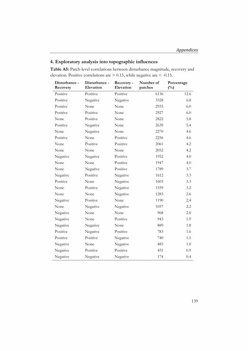
Appendices
139
4. Exploratory analysis into topographic influences
Table A5: Patch-level correlations between disturbance magnitude, recovery and elevation. Positive correlations are > 0.15, while negative are < -0.15.
Disturbance - Recovery
Disturbance - Elevation
Recovery - Elevation
Number of patches
Percentage (%)
Positive Positive Positive 6136 12.6
Positive Negative Negative 3328 6.8
Positive None None 2933 6.0
Positive Positive None 2927 6.0
None Positive None 2822 5.8
Positive Negative None 2639 5.4
None Negative None 2270 4.6
Positive None Positive 2256 4.6
None Positive Positive 2061 4.2
None None None 2052 4.2
Negative Negative Positive 1952 4.0
None None Positive 1947 4.0
None Negative Positive 1789 3.7
Negative Positive Negative 1612 3.3
Positive None Negative 1603 3.3
None Positive Negative 1559 3.2
None None Negative 1283 2.6
Negative Positive None 1190 2.4
None Negative Negative 1057 2.2
Negative None None 968 2.0
Negative None Positive 943 1.9
Negative Negative None 889 1.8
Positive Negative Positive 783 1.6
Positive Positive Negative 740 1.5
Negative None Negative 483 1.0
Negative Positive Positive 451 0.9
Negative Negative Negative 174 0.4

Appendices
140

141
Summary A third of the land on earth is covered by forests. Forests provide valuable resources and essential ecosystem services, including filtering air and water, harbouring biodiversity and managing the carbon cycle. Regular monitoring and reporting across various indicators is necessary to manage forests sustainably. Due to the vastness of forests, satellite Earth observation is one of the most practical and cost-effective ways to monitor forests. The regular and consistent measurements provided from space enable time series analysis, which can reveal trends over time. The temporal, spatial and radiometric depth of the Landsat archive, which extends back to 1972 in some cases, is one of the most useful resources for monitoring forest dynamics across large areas.
Analysing forest disturbance and recovery trends using Landsat has recently become widespread, particularly since the opening of the image archive in 2008. However, deriving useful information from the data is challenging on many fronts, including overcoming cloud-cover, differentiating true changes from noise and relating spectral measurements to meaningful outputs. In addition, large data volumes create hurdles for processing and storage. This study presents new techniques for exploiting the Landsat archive in relation to monitoring and measuring forest disturbance and recovery across large areas. Landsat data were processed through a series of steps, analysed in time series, and combined with other data sources to produce mapped outputs and statistical summaries, which can be interpreted by non-experts. The spatial extent of the analysis expands across multiple scales – from local and regional to global (temperate and boreal forests).
Firstly, eight Landsat spectral indices were assessed to determine their sensitivity to forest disturbance (caused by wildfire) and recovery in southeast Australian forests. Results indicated that indices making use of the shortwave infrared wavelengths were more reliable indicators of forest disturbance and recovery than indices using only the red and near-infrared wavelengths. Following this exploratory analysis, three indices and two change detection algorithms were evaluated in terms of their ability to detect forest disturbance. Results showed that the LandTrendr algorithm with the Normalised Burn

Summary
142
Ratio (NBR) was the most accurate single algorithm/index combination (overall error 21%). However, results were greatly improved by using an ensemble approach. A Random Forests model combining several Landsat-derived metrics with multiple indices, trained with human interpreted reference data, had an overall error of 7%. A notable finding was that priming the training data with confusing cases (commission errors from the change detection algorithms) led to increased accuracy.
One Random Forests model was used to create annual forest disturbance maps (1989-2017) across the state of Victoria, Australia. These maps, in conjunction with each pixel’s temporal trajectory, were used to extract metrics for spectral disturbance magnitude and recovery length across 2 million ha of burned forest in southeast Australia. The association between disturbance magnitude and forest recovery length, as measured spectrally, was then explored. A novel patch-based technique was used to isolate the disturbance-recovery relationship from confounding factors such as climate, elevation and soil type. The results showed statistically significant differences across bioregions and forest types. The patch-based method demonstrated how Landsat time series can be harnessed to explore ecological changes.
The methods developed above were then employed over a much larger area, to investigate trends in fire disturbance and forest recovery in temperate and boreal forests worldwide. This work used both MODIS and Landsat data, through the Google Earth Engine platform, to look at trends in burned area, fire severity and forest recovery across almost 2 billion ha of forests, over the last 18 years. Burned area results showed significant increasing trends in two cases: coniferous forests in Canada and Mediterranean forests in Chile. A significant decreasing trend was found in temperate mixed forests in China. An assessment of fire severity, as measured by Landsat spectral change, highlighted possible trends in a few cases; most notably, the Russian taiga, where increasing severity was observed. An analysis of forest recovery, based on Landsat time series, indicated recovery times were accelerating in many regions. However, given the relatively short time-period analysed, these results should be interpreted with caution.

Summary
143
The results presented in this thesis demonstrate the power of Earth observation satellites in monitoring forests at the landscape scale. Although forests are complex systems that are influenced by a myriad of factors, the regular and consistent measurements provided by satellites can be analysed in time series to provide inter-comparable results across large areas. This can broaden our understanding of the dynamic nature of forests, and in doing so, help progress towards their sustainable management.

Summary
144

145
Samenvatting Een derde van het land op aarde is bedekt met bossen. Bossen leveren waardevolle hulpbronnen en essentiële ecosysteemdiensten, waaronder het filteren van lucht en water, herbergen van biodiversiteit en het beheer van de koolstofcyclus. Het regelmatig monitoren van bossen en rapportage over verschillende indicatoren zijn nodig om bossen duurzaam te beheren. Vanwege de uitgestrektheid van bossen is satellietobservatie één van de meest praktische en kosteneffectieve manieren om bossen te monitoren. De regelmatige en consistente metingen vanuit de ruimte maken tijdreeksanalyses mogelijk, waaruit trends kunnen worden gedestilleerd. De temporele, ruimtelijke en radiometrische diepte van het Landsat-archief , dat in sommige gevallen teruggaat tot 1972, is een van de meest bruikbare bronnen voor het volgen van bosdynamiek in grote gebieden.
Het analyseren van bosverstoringen en hersteltrends met Landsat is recentelijk een wijdverspreide praktijk geworden, vooral sinds het beeldarchief openbaar toegankelijk werd in 2008. Het is echter op veel fronten een uitdaging om bruikbare informatie uit de gegevens te halen, waaronder het overwinnen van data ruis door bewolking, het onderscheiden van echte veranderingen van ruis en spectrale metingen aan betekenisvolle outputs. Bovendien creëren de grote datavolumes hindernissen voor verwerking en opslag van geanalyseerde data. Deze studie presenteert nieuwe technieken voor het exploiteren van het Landsat-archief met betrekking tot het monitoren en meten van bosverstoring en herstel in grote gebieden. Landsat-gegevens werden verwerkt via een reeks stappen, geanalyseerd in tijdreeksen en gecombineerd met andere gegevensbronnen om in kaart gebrachte resultaten en statistische samenvattingen te produceren, die ook door niet-experts kunnen worden geïnterpreteerd. De ruimtelijke omvang van de analyse breidt zich uit over meerdere schalen - van lokaal en regionaal tot mondiaal (gematigde en boreale bossen).
Eerst werden acht Landsat spectrale indices beoordeeld opm hun gevoeligheid voor om bosverstoring (veroorzaakt door bosbranden) en herstel in zuidoost-Australische bossen te bepalen. De resultaten wezen erop dat indices die gebruikmaken van de kortegolf-infrarood-golflengten

Samenvatting
146
betrouwbaardere indicatoren waren voor bosverstoring- en herstel, dan indices die alleen de rode en nabij-infrarode golflengten gebruikten. Na deze verkennende analyse werden drie indices en twee veranderings-detectiealgoritmen beoordeeld op hun vermogen om bosverstoringen te detecteren. De resultaten toonden aan dat het LandTrendr-algoritme met de genormaliseerde verbrandingsratio (NBR) de meest nauwkeurige combinatie van algoritmen en indexen was (totale foutmarge 21%). De resultaten werden echter sterk verbeterd door gebruik te maken van een ensemble benadering. Een model in willekeurige bossen gecombineerd met verschillende Landsat-afgeleide metrieken met meerdere indices, getraind met de door mensen geïnterpreteerde referentiegegevens, had een totale foutmarge van 7%. Een opmerkelijke bevinding was dat het bewerken van de trainingsgegevens met verwarrende zaken (provisiefouten van de algoritmen voor wijzigingsdetectie) tot een grotere nauwkeurigheid leidde.
Het One Random Forests-model werd gebruikt om jaarlijkse bosverstoringskaarten (1989-2017) te maken in de staat Victoria, Australië. Deze kaarten, in combinatie met het temporele traject van elke pixel, werden gebruikt om metrieken te extraheren voor de spectrale verstoringsgrootte en de herstellengte over 2 miljoen hectare verbrand bos in Zuidoost-Australië. De associatie tussen de verstoringsgrootte en bosherstellengte, zoals spectraal is gemeten, werd vervolgens onderzocht. Een nieuwe patch-gebaseerde techniek werd gebruikt om de relatie tussen verstoring en herstel te isoleren van verstorende factoren zoals klimaat, hoogte en bodemtype. De resultaten toonden statistisch significante verschillen tussen bio-regio's en bostypen. De patch-gebaseerde methode laat zien hoe Landsat-tijdreeksen kunnen worden gebruikt om ecologische veranderingen te onderzoeken.
De hierboven ontwikkelde methoden werden vervolgens voor een veel groter gebied gebruikt om trends in bosverstoring door brand en bosherstel in gematigde en boreale bossen over de hele wereld te onderzoeken. In dit onderzoek werden zowel MODIS- als Landsat-gegevens gebruikt, via het Google Earth Engine-platform, om de afgelopen 18 jaar te kijken naar trends in verbrand gebied, ernst van de brand en bosherstel in bijna 2 miljard hectare bos. De gebiedsresultaten toonden aanzienlijke stijgende trends in twee gevallen: naaldbossen in Canada en mediterrane bossen in Chili. Een

Samenvatting
147
significante afnemende trend werd gevonden in gematigde gemengde bossen in China. Een beoordeling van de ernst van de brand, op basis van Landsat’s spectrale veranderingsmetingen, benadrukte mogelijke trends in een paar gevallen; met name in de Russische taiga, waar toenemende ernst van bosbranden werd waargenomen. Uit een analyse van bosherstel, gebaseerd op Landsat-tijdreeksen, bleek dat in veel regio's de hersteltijden aan het versnellen waren. Gezien de relatief korte geanalyseerde periode, moeten deze resultaten echter met de nodige voorzichtigheid worden geïnterpreteerd.
De resultaten die in dit proefschrift worden gepresenteerd, tonen de kracht van aardobservatiesatellieten bij het volgen van bossen op landschapsschaal. Hoewel bossen complexe systemen zijn die worden beïnvloed door een groot aantal factoren, kunnen de regelmatige en consistente metingen van satellieten worden geanalyseerd in tijdreeksen om vergelijkbare resultaten voor grote gebieden te bieden. Dit kan ons begrip van de dynamische aard van bossen verruimen en daarmee bijdragen aan hun duurzaam beheer.


