Using GIS-GPS Devices with Thermo Scientific Niton XRF Analyzers

Standard Operating Procedure

October 2011

2

TABLE OF CONTENTS

Adding Niton XRF Applet to ArcPad…………………………………………………….. 3 Bluetooth Connection of Thermo Scientific XRF and Trimble…….……..……. 5 Geo-Mapping & Elemental Mapping – Thermo Scientific Niton XRF and Trimble-Discover Mobile….………………… 8 Geo-Mapping & Elemental Mapping – Thermo Scientific Niton XRF and Trimble-ArcPad ……..………………………..… 19 Presentation of Assay Data with GPS Coordination in Google Earth..…..… 26 Presentation of Assay Data with GPS Coordination in ArcPad…………..…… 28 Bluetooth Connection of Trip Recorder 747 Pro GPS to Thermo Scientific Niton XRF……………………….….………………………………….. 32

3

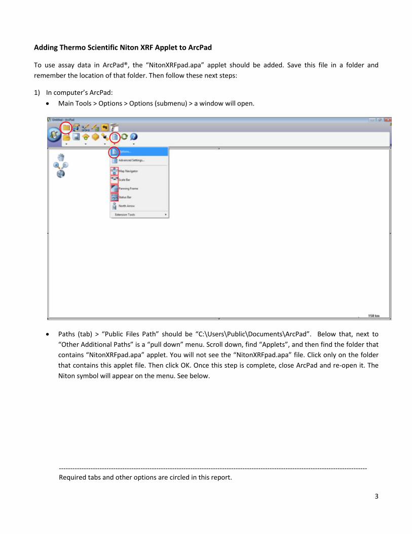
Adding Thermo Scientific Niton XRF Applet to ArcPad

To use assay data in ArcPad®, the “NitonXRFpad.apa” applet should be added. Save this file in a folder and remember the location of that folder. Then follow these next steps:

1) In computer’s ArcPad: • Main Tools > Options > Options (submenu) > a window will open.

• Paths (tab) > “Public Files Path” should be “C:\Users\Public\Documents\ArcPad”. Below that, next to “Other Additional Paths” is a “pull down” menu. Scroll down, find “Applets”, and then find the folder that contains “NitonXRFpad.apa” applet. You will not see the “NitonXRFpad.apa” file. Click only on the folder that contains this applet file. Then click OK. Once this step is complete, close ArcPad and re-open it. The Niton symbol will appear on the menu. See below.

---------------------------------------------------------------------------------------------------------------------------------------- Required tabs and other options are circled in this report.

4

2) In Trimble ArcPad: • Connect Trimble® to the computer by USB cable. • Find and open Trimble, and then save the “NitonXRFpad.apa” applet in “My Documents” (copy and

paste the applet file from computer to “My Documents” in Trimble). • Follow the steps above to add the applet to ArcPad in Trimble.

5

Bluetooth Connection of Thermo Scientific Niton XRF Analyzer and Trimble

1) Turn on both the Thermo Scientific Niton analyzer and Trimble 2) In Trimble:

a. If the instrument had previously connected to Trimble, follow this step: I. Start > Settings > Connections (tab) > Wireless Manager > Bluetooth™ > ON. Bluetooth

“Visible” will appear.

b. If this is the first time pairing the analyzer with Trimble, follow these steps:

I. Start > Settings > Connections (tab) > Wireless Manager > Menu (tab) > Bluetooth settings > Mode (tab) > Check “Turn on Bluetooth” and also “Make this device visible to other devices” > Click “ok” (top right corner); then Bluetooth “Visible” will appear in next window.

6

II. In COM Ports tab, choose the “Incoming Port (COM9)”. If it is other than this port, tap it > Edit > in the new window, select COM9 in drop down menu under Port. Also uncheck “Secure Connection”. If it is checked, when the analyzer finds Trimble, a message comes in Trimble

III. Then “Finish” (bottom right corner > Click “ok” (top right corner); then Bluetooth “Visible” will appear in next window

informing “….(name of the device) wants to connect to your device using Bluetooth. Do you want to ….?”, click “Yes”, then it will ask for password, which is 0000; then click “Next”. Now the analyzer and Trimble are connected. The analyzer should show a blinking blue light.

IV. NOTE: If no port is listed in the Incoming Port, a Bluetooth incoming serial Port CAB file needs

to be loaded onto the Trimble Juno. This file is supplied from Trimble directly and is free of charge. Install the BluetoothIncomingSerialPort.cab file for Trimble mobile devices. This allows the external sensor to become the Bluetooth Host, and the Trimble mobile device becomes the client. To do this: 1. Go to www.trimble.com and then select Support & Training / Support A-Z list. 2. Select the required device from the list. http://www.trimble.com/junosb_ts.asp 3. Navigate to the Downloads page, locate the cab file and then save it to the office computer. http://trl.trimble.com/dscgi/ds.py/Get/File-504041/BluetoothIncomingSerialPort.cab 4. Connect the mobile device to the office computer using the Microsoft® ActiveSync® technology, or the Windows Mobile Device Centre. 5. On the office computer, copy the cab file to the My Documents folder on the mobile device. 6. On the mobile device, tap the BluetoothIncomingSerialPort.cab file.

7

The file installs silently on the mobile device without any user notification, and the port COM9: Bluetooth is created for external sensors.

3) On the Thermo Scientific Niton analyzer: b. Turn on and Log in c. System > Bluetooth > Enable d. If this is the first time pairing the analyzer with Trimble, follow these steps:

I. System > Bluetooth > Search. It may take a few minutes until the analyzer “finds” the Trimble. After finding, click on the name of GIS device (Trimble).

II. Config > Type (scroll down) > GIS > Save > Connect. Now the analyzer should be trying to connect to Trimble. If it fails to connect, try again to “Connect”. Now it is connected to Trimble. If you try a few times and it fails to connect, follow these steps:

a. Trimble: Turn off and on again b. Analyzer: System > Bluetooth > Reset > Search > Connect (after finding Trimble)

III. A message that the analyzer is connected to Trimble will appear on the screen.

e. If the analyzer has been previously connected to this Trimble, follow these steps:

System > Bluetooth > Click on the name of Trimble unit > follow steps in step III above.

f. For printing, follow these steps:

System > Printer > check these “Auto Print Readings”, “Print Complete”, “Print Data Fields”

8

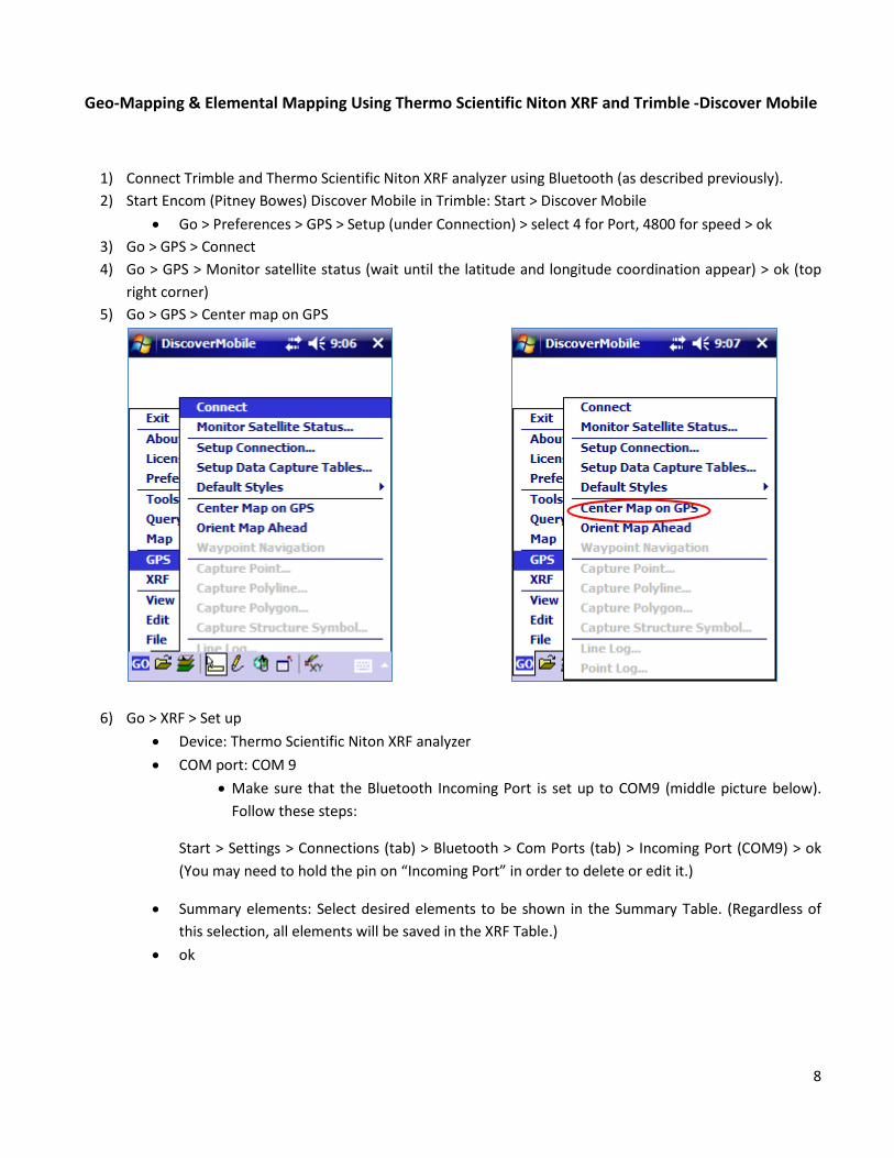
Geo-Mapping & Elemental Mapping Using Thermo Scientific Niton XRF and Trimble -Discover Mobile

1) Connect Trimble and Thermo Scientific Niton XRF analyzer using Bluetooth (as described previously). 2) Start Encom (Pitney Bowes) Discover Mobile in Trimble: Start > Discover Mobile

• Go > Preferences > GPS > Setup (under Connection) > select 4 for Port, 4800 for speed > ok 3) Go > GPS > Connect 4) Go > GPS > Monitor satellite status (wait until the latitude and longitude coordination appear) > ok (top

right corner) 5) Go > GPS > Center map on GPS

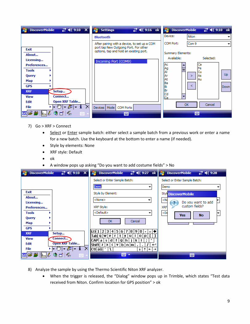
6) Go > XRF > Set up • Device: Thermo Scientific Niton XRF analyzer • COM port: COM 9

• Make sure that the Bluetooth Incoming Port is set up to COM9 (middle picture below). Follow these steps:

Start > Settings > Connections (tab) > Bluetooth > Com Ports (tab) > Incoming Port (COM9) > ok (You may need to hold the pin on “Incoming Port” in order to delete or edit it.)

• Summary elements: Select desired elements to be shown in the Summary Table. (Regardless of this selection, all elements will be saved in the XRF Table.)

• ok

9

7) Go > XRF > Connect • Select or Enter

• Style by elements: None

sample batch: either select a sample batch from a previous work or enter a name for a new batch. Use the keyboard at the bottom to enter a name (if needed).

• XRF style: Default • ok • A window pops up asking “Do you want to add costume fields” > No

8) Analyze the sample by using the Thermo Scientific Niton XRF analyzer. • When the trigger is released, the “Dialog” window pops up in Trimble, which states “Test data

received from Niton. Confirm location for GPS position” > ok

10

• The “XRF Data Explore” window will appear with 6 tabs: Information, Summary (showing the summary elements selected in 6c), XRF data 1, XRF data 2, XRF data 3, Geography. All elements (depending on the elements) will be in the XRF data tabs.

• NOTE: If this window is closed, you cannot go back to it in Trimble. However, the data will be there to be used. Also, data can be downloaded to computer. See below for instructions.

• ok (on the top right corner) • A window pops up asking “Use a named style” > No • A window pops up asking “Edit attributes” > No • Now the location of the sample appears in the map in the main window of Discover Mobile.

• You may use and point to the sample in the map to view the data.

• Conduct all analyses following steps 8a to 8f.

i

11

• NOTE: If the satellite signal is lost, a window appears asking “Try Again”. Click on “Try Again”. Trimble will connect to the satellite and record coordination for that analysis. There is no need to repeat that analysis. “Try Again” is only for the satellite connection.

• To show the GPS coordination as Universal Transverse Mercator (UTM) in the gridlines of the map: Go > Map > Map Projection > under “Category” select Universal Transverse

Mercator (WGS 84) > under “Category members” select appropriate UTM Zone based on the geographic location of the area (for example, Boston is UTM Zone 19, Northern Hemisphere) > Ok.

To see the UTM grid lines: Go > GPS > Center Map on GPS 9) Saving the layer in Trimble: This stage is important in order to make maps in Trimble.

• Go > File > “Save Table Copy as”. • Layer: Will be the same as that in 7a • File: Name it as desired (e.g., “Demo.tab”) and save it in “My Documents”. This will be the

.tab file that you will need later to make map(s) by MapInfo on your computer or Trimble. • There are other fields. No need to change them at this stage. • ok (top right corner)

10) Connect Trimble to your computer using a USB cable. • Open “My Computer” and open the Trimble folder. • My documents > you will see 5 different files with the same name as that in 9a (e.g., “Demo”).

These files are: one “DAT File”, three “MapInfo Table File”, one “MapInfo Table”. All these files are needed. Create a folder on your computer (e.g., desktop) and copy-paste these files to that folder.

• NOTE: These files are also saved in a folder (with same name as that in 7a) in the “Niton” folder. So if step 9 was missed, the files can be accessed from this folder.

12

• Double-click (open) the “MapInfo Table” file. It will open in MapInfo.

11) To show Table of assays: • “Map” in menu > Layer Control > (Layer Control window on left-hand side appears) > right click on

the layer (“Project” in this example) > Browse Table > Table with all analysis and coordination will appear.

13

14

12) Geo-mapping: To show the location of samples on the Earth: • File > Tile Sever Maps > Add Bing Aerial to Map

15

13) Elemental mapping using MapInfo on the computer: • “Map” in menu > Create Thematic Map. A window (Create Thematic Map – Step 1 of 3) appears.

In this window, Select the desired method of elemental mapping, e.g., Type: Ranges > Template Name: “Region Ranges, Solid Red-Yellow-Green” > Next

• Another window (Create Thematic Map – Step 2 of 3) appears where you select Table (e.g., “Project” in the example), and Field (the desired element) > Next

• In next window (Create Thematic Map – Step 3 of 3), select desired options for ranges, styles, legend, color, font > OK

• The selected element’s map will appear. • You may modify the map: Map > Modify Thematic Map > select Thematic layer (the

elemental map layer, e.g., Cu) > Modify > Styles (in the Modify Thematic Map window) > check “All Attributes” under “Apply”. You can also click on the symbol and change its shape and color, as desired.

16

17

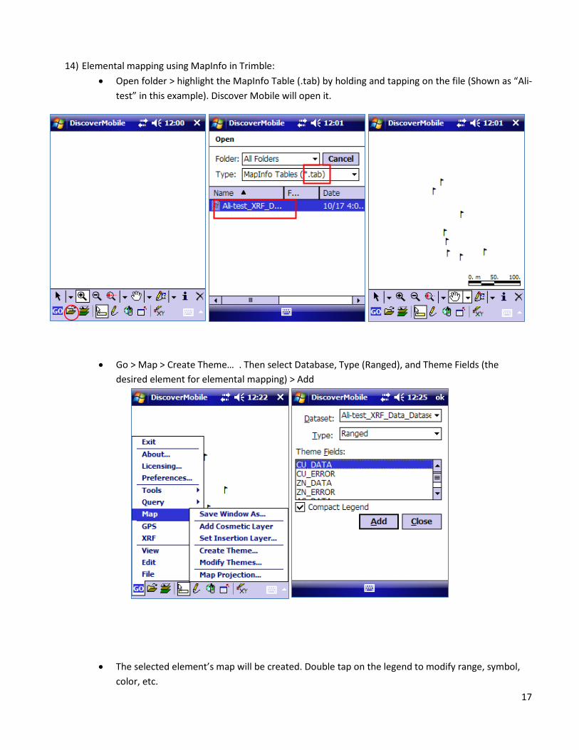
14) Elemental mapping using MapInfo in Trimble: • Open folder > highlight the MapInfo Table (.tab) by holding and tapping on the file (Shown as “Ali-

test” in this example). Discover Mobile will open it.

• Go > Map > Create Theme… . Then select Database, Type (Ranged), and Theme Fields (the desired element for elemental mapping) > Add

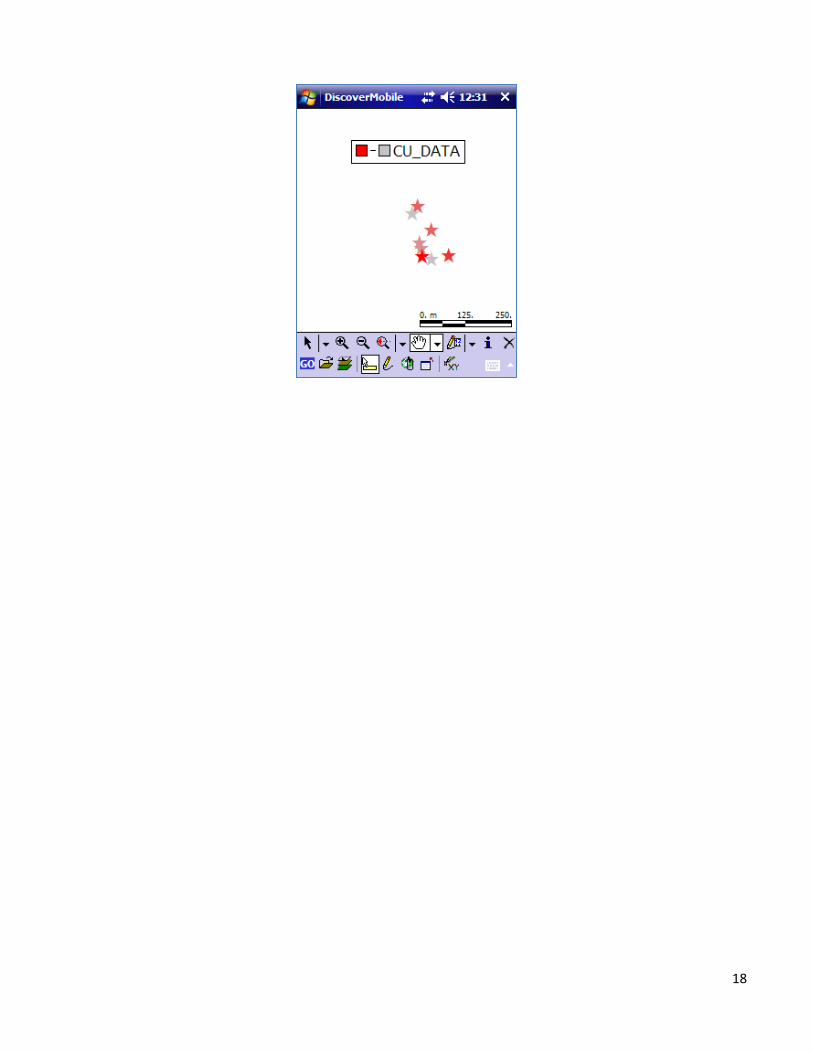
• The selected element’s map will be created. Double tap on the legend to modify range, symbol, color, etc.

18

19

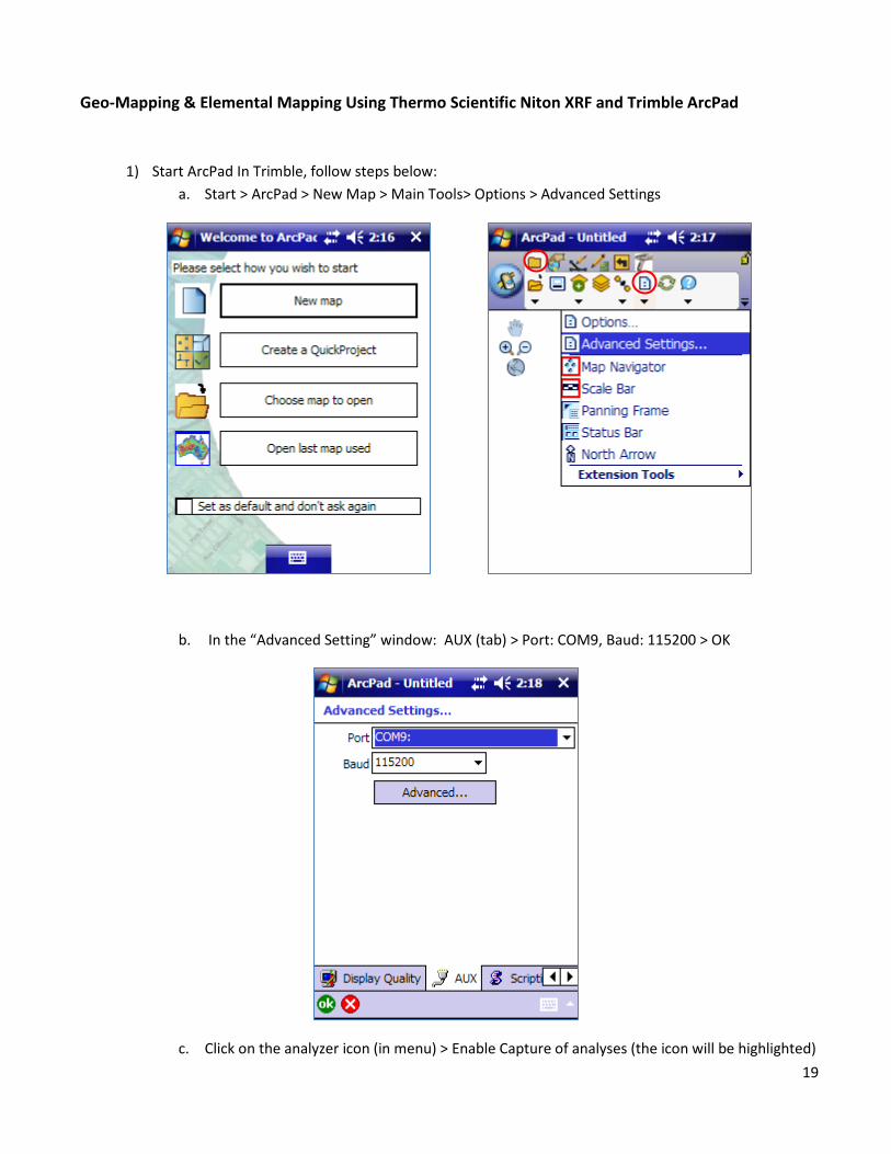
Geo-Mapping & Elemental Mapping Using Thermo Scientific Niton XRF and Trimble ArcPad

1) Start ArcPad In Trimble, follow steps below: a. Start > ArcPad > New Map > Main Tools> Options > Advanced Settings

b. In the “Advanced Setting” window: AUX (tab) > Port: COM9, Baud: 115200 > OK

c. Click on the analyzer icon (in menu) > Enable Capture of analyses (the icon will be highlighted)

20

d. Click on “Manage Analysis Layers” > Create New (in the XRF Analysis Layers window) > Check desired elements, units, and mode (tab) in the XRF Mode Selection window. For example:

i. Create New > Mining Cu/Zn mode > check “Ni” (and any other elements) > check “PPM” (Units) > ok

ii. Highlight the desired element for elemental mapping > ok > Choose ”Symbol”, “Color By Element” and “Number of Ranges” > ok > Choose desired ranges > ok > Save the file

21

iii. If you like to use an existing layer, follow these steps: “Manage Analysis Layers” > Add Existing > click on the desired layer (then this layer will be added to the Active layers list)

2) In the field: a. In Trimble ArcPad, follow these steps:

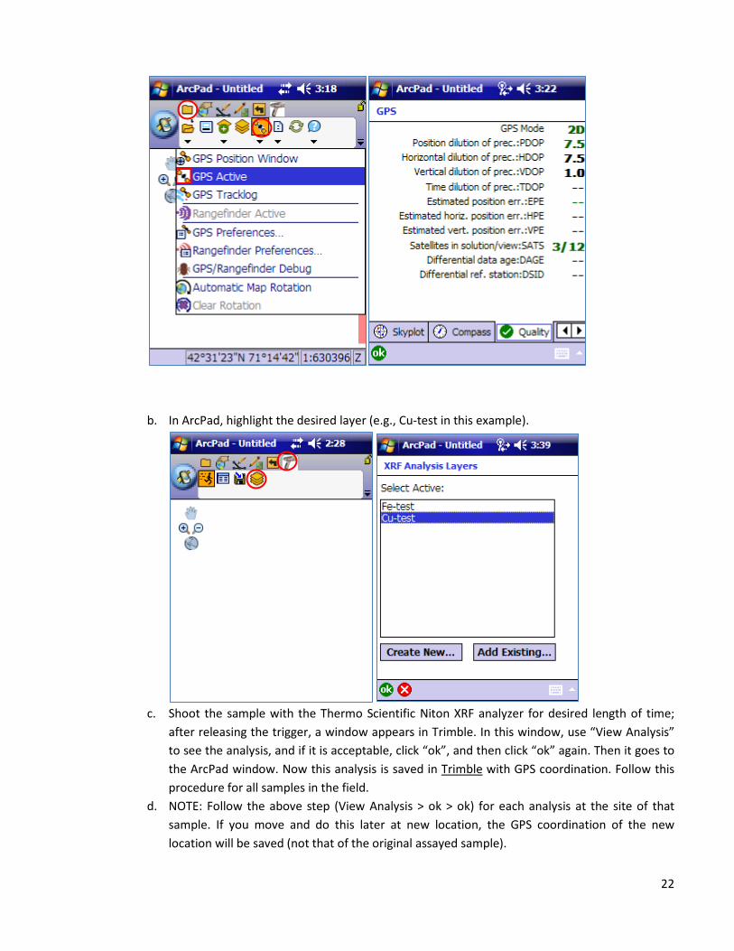
Main Tools > GPS Active (menu) > GPS Active > GPS Position Window (a window will open with a few submenus. Use the “Quality” tab to see the number of “Satellites in solution/view”. This should be at least 3/12. After getting enough satellites (at least 3), start using the analyzer.

22

b. In ArcPad, highlight the desired layer (e.g., Cu-test in this example).

c. Shoot the sample with the Thermo Scientific Niton XRF analyzer for desired length of time;

after releasing the trigger, a window appears in Trimble. In this window, use “View Analysis” to see the analysis, and if it is acceptable, click “ok”, and then click “ok” again. Then it goes to the ArcPad window. Now this analysis is saved in Trimble

d. NOTE: Follow the above step (View Analysis > ok > ok) for each analysis at the site of that sample. If you move and do this later at new location, the GPS coordination of the new location will be saved (not that of the original assayed sample).

with GPS coordination. Follow this procedure for all samples in the field.

23

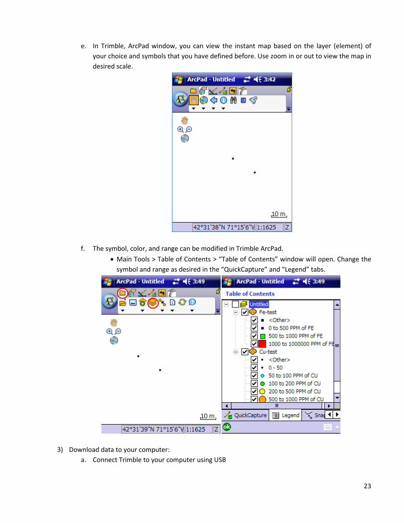
e. In Trimble, ArcPad window, you can view the instant map based on the layer (element) of your choice and symbols that you have defined before. Use zoom in or out to view the map in desired scale.

f. The symbol, color, and range can be modified in Trimble ArcPad. • Main Tools > Table of Contents > “Table of Contents” window will open. Change the

symbol and range as desired in the “QuickCapture” and “Legend” tabs.

3) Download data to your computer: a. Connect Trimble to your computer using USB

24

b. Find Trimble in the computer: My Computer > Trimble > My Documents > Download (e.g., by copy and paste) files (that were created during the use of the Trimble in the field) into “My Documents”.

• NOTE: For each map, four files (APL, DBF, SHP, SHX) are created and all of them are necessary to open a map. If any of them is deleted, ArcPad will not open the map.

• Do not rename these four files (APL, DBF, SHP, SHX). ArcPad will not open the map.

c. In “My Documents” double click the file (either “Shape” file with extension .shp or “Map” file with extension .apm). It will be opened by ArcPad. If not, right click on the file > “Open with” > ArcPad. (You may need to find ArcPad program in your computer and click on it.)

• Use Zoom in/out (scroll with the mouse) to see the analyzed sites in desired scale. You may save this as a “Map”. The ArcPad Map (APM) file can be named differently.

d. Viewing data and changing symbol: This can be done in two ways: • Main Tools > Table of Contents > A window will open. Change the symbol and range

as desired in the “QuickCapture” and “Legend” submenus. • Quick Capture > Click on the symbol > double click on any analyzed point, a window

will open showing the data for that point. 1. “Symbology” tab > click on Symbol sign > click on Symbol tab > chose desired

symbol > ok > ok

25

26

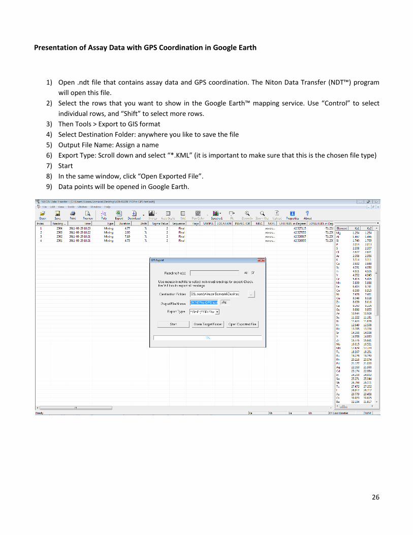
Presentation of Assay Data with GPS Coordination in Google Earth

1) Open .ndt file that contains assay data and GPS coordination. The Niton Data Transfer (NDT™) program will open this file.

2) Select the rows that you want to show in the Google Earth™ mapping service. Use “Control” to select individual rows, and “Shift” to select more rows.

3) Then Tools > Export to GIS format 4) Select Destination Folder: anywhere you like to save the file 5) Output File Name: Assign a name 6) Export Type: Scroll down and select “*.KML” (it is important to make sure that this is the chosen file type) 7) Start 8) In the same window, click “Open Exported File”. 9) Data points will be opened in Google Earth.

27

28

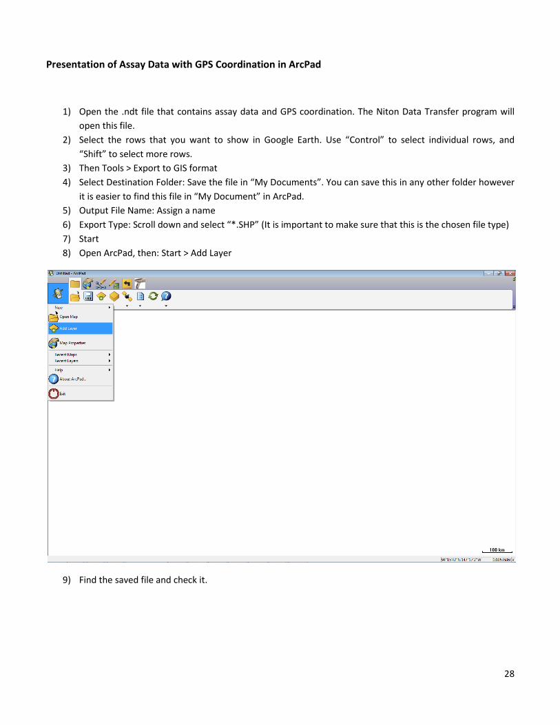
Presentation of Assay Data with GPS Coordination in ArcPad

1) Open the .ndt file that contains assay data and GPS coordination. The Niton Data Transfer program will open this file.

2) Select the rows that you want to show in Google Earth. Use “Control” to select individual rows, and “Shift” to select more rows.

3) Then Tools > Export to GIS format 4) Select Destination Folder: Save the file in “My Documents”. You can save this in any other folder however

it is easier to find this file in “My Document” in ArcPad. 5) Output File Name: Assign a name 6) Export Type: Scroll down and select “*.SHP” (It is important to make sure that this is the chosen file type) 7) Start 8) Open ArcPad, then: Start > Add Layer

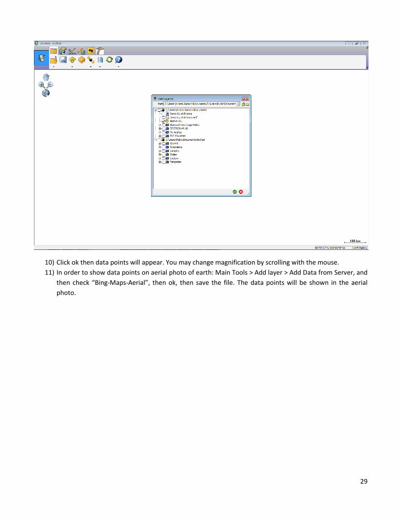
9) Find the saved file and check it.

29

10) Click ok then data points will appear. You may change magnification by scrolling with the mouse. 11) In order to show data points on aerial photo of earth: Main Tools > Add layer > Add Data from Server, and

then check “Bing-Maps-Aerial”, then ok, then save the file. The data points will be shown in the aerial photo.

30

31

12) Now there are 2 layers, one the data points and one the aerial map. Use Main Tools > Table of Contents to check/uncheck any desired layer.

32

Bluetooth Connection of Trip Recorder 747 Pro GPS to Thermo Scientific Niton XRF Analyzer

1) Turn on Trip Recorder 747 Pro GPS. The blue light will blink. Make sure it is charged. Follow the instructions in the device manual for charging.

2) On the analyzer:

a. Turn on and Log in b. System > Bluetooth c. If this is the first time pairing the analyzer with Trimble, follow these steps:

• System > Bluetooth > Search. It may take a few minutes until the analyzer “finds” Trip Recorder 747 Pro. After finding, click on the name of GPS device (Trip Recorder 747 Pro). Then Config > Type (scroll down) > GPS > Save > Connect. It may take 1-2 minutes; after the connection is made, the orange light on the GPS device will turn on, while the blue light will blink on both the analyzer and GPS.

i. If the analyzer has been previously connected to this device, follow these steps:

System > Bluetooth > Click on the name of device > Connect

ii. Click on “GPS” and wait till “Lat” and “Long” numbers appear. d. Assay sample: Each time that the trigger is released, the GPS coordination is recorded in the NDT

file. As long as there is a Bluetooth connection and the GPS is receiving satellite signals, the GPS coordination will be recorded in the NDT file.

• NOTE: GPS coordination is not displayed in the analyzer’s analysis table.

33

©2011 Thermo Fisher Scientific Inc. All rights reserved. ArcPad is a registered trademark of Esri in the United States, the European Community, or certain other jurisdictions. Bluetooth is a trademark of Bluetooth SIG, Inc. Trimble is a registered trademark of Trimble Navigation Limited. MapInfo is a registered trademark of Pitney Bowes MapInfo Corporation. Google Earth is a trademark of Google Inc. All other trademarks are the property of Thermo Fisher Scientific Inc. and its subsidiaries.

Specifications, terms and pricing are subject to change. Not all products are available in all countries. Please consult your local sales representative for details.

Figure on the cover page courtesy of www.worldatlas.com