1/33

Using Local Spectral Methodsin Theory and in Practice

Michael W. Mahoney

ICSI and Dept of Statistics, UC Berkeley

( For more info, see:http: // www. stat. berkeley. edu/ ~ mmahoney

or Google on “Michael Mahoney”)

December 2015

2/33

Global spectral methods

Given the Laplacian L of a graph G = (V ,E ), solve the following:

minimize xTLx

subject to xTDx = 1

xTD1 = 0

Good News: Things one can prove about this.

I Solution can be found by computing an eigenvector of L.

I Solution can be found by running a random walk to ∞.

I Solution is “quadratically good” (i.e., Cheeger’s Inequality).

I Solution can be used for clustering, classification, ranking, etc.

Bad News: This is a very global thing and so often not useful.

I Can we localize it in some meaningful way?

Outline

Motivation 1: Social and information networks

Motivation 2: Machine learning data graphs

Local spectral methods in worst-case theory

Local spectral methods to robustify graph construction

3/33

4/33

Networks and networked data

Lots of “networked” data!!

I technological networks (AS,power-grid, road networks)

I biological networks (food-web,protein networks)

I social networks (collaborationnetworks, friendships)

I information networks(co-citation, blog cross-postings,advertiser-bidded phrase graphs...)

I language networks (semanticnetworks ...)

I . . .

Interaction graph model of networks:

I Nodes represent “entities”

I Edges represent “interaction”between pairs of entities

5/33

Three different types of real networks

100 101 102 103 10410−3

10−2

10−1

100

size

conductance

CA-GrQc

FB-Johns55

US-Senate

(a) NCP: conductance value of bestconductance set, as function of size

100 101 102 103 10410−3

10−2

10−1

100

101

102

size

conductance

ratio

CA-GrQc

FB-Johns55

US-Senate

(b) CRP: ratio of internal to externalconductance, as function of size

(c) CA-GrQc (d) FB-Johns55

00.51

(e) US-Senate

6/33

Information propagates local-to-glocal in different networksin different ways

Figure: Top: CA-GrQc; Middle: FB-Johns55; Bottom: US-Senate.

Outline

Motivation 1: Social and information networks

Motivation 2: Machine learning data graphs

Local spectral methods in worst-case theory

Local spectral methods to robustify graph construction

7/33

8/33

Use case1: Galactic spectra from SDSS

xi ∈ R3841, N ≈ 500k

photon fluxes in ≈ 10 Awavelength bins

preprocessing corrects forredshift, gappy regions

normalized by median fluxat certain wavelengths

3000 4000 5000 6000 7000 8000 90000

2

4

6raw spectrum in observed frame

3000 4000 5000 6000 7000 8000 90000

2

4

6raw spectrum in rest frame

3000 4000 5000 6000 7000 8000 90000

2

4

6gap−corrected spectrum in rest frame

1Also results in neuroscience as well as genetics and mass spec imaging.

9/33

Red vs. blue galaxies

(a) red galaxy image (b) blue galaxy image

(c) red galaxy spectrum (d) blue galaxy spectrum

10/33

Dimension reduction in astronomy

An incomplete history:

I (Connolly et al., 1995): principal components analysis

I (Vanderplas & Connolly, 2009): locally linear embedding

I (Richards et al., 2009): diffusion maps regression

I (Yip, Mahoney, et al., 2013): CUR low-rank decompositions

Here:

I Apply global/local spectral methods to astronomical spectra

I Address both nonlinear structure and nonuniform density

I Explore locally-biased versions of these embeddings for adownstream classification task

11/33

Constructing global diffusion embeddings(Belkin & Niyogi, 2003; Coifman & Lafon, 2006)

Given data {xj}Nj=1, form graph with edge weights

Wij = exp

(−‖xi − xj‖2

εiεj

), Dii =

∑j

Wij

In practice, only add k nearest-neighbor edges

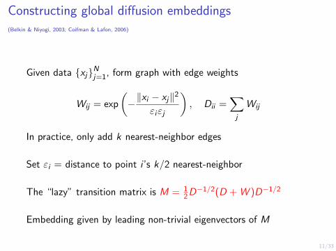
Set εi = distance to point i ’s k/2 nearest-neighbor

The “lazy” transition matrix is M = 12D

−1/2(D + W )D−1/2

Embedding given by leading non-trivial eigenvectors of M

12/33

Global embedding: effect of k

Figure: Eigenvectors 3 and 4 of Lazy Markov operator, k = 2 : 2048

13/33

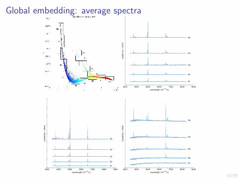
Global embedding: average spectra

3000 4000 5000 6000 7000 8000 9000

A1

A2

A3

A4

A5

wavelength (10−10

m)

scale

d flu

x +

offset

3000 4000 5000 6000 7000 8000 9000

E1

E2

E3

E4

E5

wavelength (10−10

m)

scale

d flu

x +

offset

3000 4000 5000 6000 7000 8000 9000

R1

R2

R3

R4

R5

wavelength (10−10

m)

scale

d flu

x +

offset

14/33

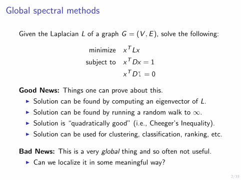
Optimization approach to global spectral methods

Markov matrix related to combinatorial graph Laplacian L:

Ldef= D −W = 2D1/2(I −M)D1/2

Can write v2, the first nontrivial eigenvector of L, as the solution to

minimize xTLx

subject to xTDx = 1

xTD1 = 0

Similarly for vt with additional constraints xTDvj = 0, j < t.

Theorem. Solution can be found by computing an eigenvector. Itit is “quadratically good” (i.e., Cheeger’s Inequality).

15/33

MOV optimization approach to local spectral methods(Mahoney, Orecchia, and Vishnoi, 2009; Hansen and Mahoney, 2013; Lawlor, Budavari, Mahoney, 2015)

Suppose we have:

1. a seed vector s = χS , where S is a subset of data points

2. a correlation parameter κ

MOV objective. The first semi-supervised eigenvector w2 solves:

minimize xTLx

subject to xTDx = 1

xTD1 = 0

xTDs ≥√κ

Similarly for wt with addition constraints xTDwj = 0, j < t.

Theorem. Solution can be found by solving a linear equation. It is“quadratically good” (with a local version of Cheeger’s Inequality).

16/33

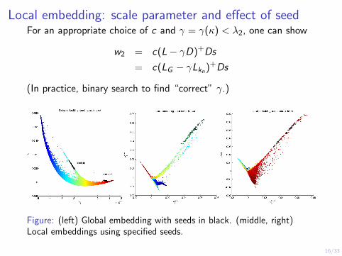
Local embedding: scale parameter and effect of seedFor an appropriate choice of c and γ = γ(κ) < λ2, one can show

w2 = c(L− γD)+Ds

= c(LG − γLkn)+Ds

(In practice, binary search to find “correct” γ.)

Figure: (left) Global embedding with seeds in black. (middle, right)Local embeddings using specified seeds.

17/33

Classification on global and local embeddings

Try to reproduce 5 astronomer-defined classes

Train multiclass logistic regression on global and local embeddings

Seeds chosen to discriminate one class (e.g., AGN) vs. rest

Figure: (left) Global embedding, colored by class. (middle, right)Confusion matrices for classification on global and local embeddings.

Outline

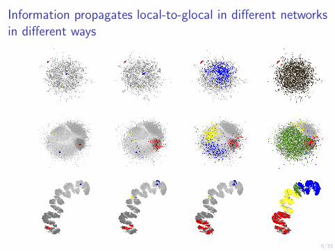
Motivation 1: Social and information networks

Motivation 2: Machine learning data graphs

Local spectral methods in worst-case theory

Local spectral methods to robustify graph construction

18/33

19/33

Local versus global spectral methods

Global spectral methods:

I Compute eigenvectors of matrices related to the graph.

I Provide “quadratically good” approximations to the bestpartitioning of the graph (Cheeger’s Inequality).

I This provide inference control for classification, regression, etc.

Local spectral methods:

I Use random walks to find locally-biased partitions in large graphs.

I Can prove locally-biased versions of Cheeger’s Inequality.

I Scalable worst-case running time; non-trivial statistical properties.

Success stories for local spectral methods:

I Getting nearly-linear time Laplacian-based linear solvers.

I For finding local clusters in very large graphs.

I For analyzing large social and information graphs.

20/33

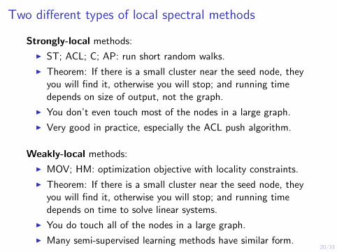
Two different types of local spectral methods

Strongly-local methods:

I ST; ACL; C; AP: run short random walks.

I Theorem: If there is a small cluster near the seed node, theyyou will find it, otherwise you will stop; and running timedepends on size of output, not the graph.

I You don’t even touch most of the nodes in a large graph.

I Very good in practice, especially the ACL push algorithm.

Weakly-local methods:

I MOV; HM: optimization objective with locality constraints.

I Theorem: If there is a small cluster near the seed node, theyyou will find it, otherwise you will stop; and running timedepends on time to solve linear systems.

I You do touch all of the nodes in a large graph.

I Many semi-supervised learning methods have similar form.

21/33

The ACL push procedure

1. ~x (1) = 0, ~r (1) = (1− β)~ei , k = 1

2. while any rj > τdj dj is the degree of node j

3. ~x (k+1) = ~x (k) + (rj − τdjρ)~ej

4. ~x(k+1)i =

τdjρ i = j

r(k)i + β(rj − τdjρ)/dj i ∼ j

r(k)i otherwise

5. k ← k + 1

Things to note:

I This approximates the solution to the personalized PageRank problem:

I (I − βAD−1)~x = (1− β)~v ;

I (I − βA)~y = (1− β)D−1/2~v , where

{A = D−1/2AD−1/2

~x = D1/2~yI [αD + L]~z = α~v , where β = 1/(1 + α) and ~x = D~z .

I The global invariant ~r = (1− β)~v − (I − βAD−1)~x is maintainedthroughout, even though ~r and ~x are supported locally.

I Question: What does this algorithm compute—approximately or exactly?

22/33

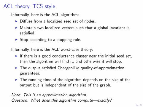
ACL theory, TCS style

Informally, here is the ACL algorithm:

I Diffuse from a localized seed set of nodes.

I Maintain two localized vectors such that a global invariant issatisfied.

I Stop according to a stopping rule.

Informally, here is the ACL worst-case theory:

I If there is a good conductance cluster near the initial seed set,then the algorithm will find it, and otherwise it will stop.

I The output satisfied Cheeger-like quality-of-approximationguarantees.

I The running time of the algorithm depends on the size of theoutput but is independent of the size of the graph.

Note: This is an approximation algorithm.Question: What does this algorithm compute—exactly?

23/33

Constructing graphs that algorithms implicitly optimize

Given G = (V ,E), add extra nodes, s and t, with weights connected to nodesin S ⊂ V or to S .

Then, the s, t-minimum cut problem is:

minxs=1,xt=0

‖B~x‖C ,1 =∑

(u,v)∈EC(u,v)|xu − xv |

The `2-minorant of this problem is:

minxs=1,xt=0

‖B~x‖C ,2 =

√ ∑(u,v)∈E

C(u,v)|xu − xv |2

or, equivalently, of this problem:

minxs=1,xt=0

1

2‖B~x‖2C ,2 =

1

2

∑(u,v)∈E

C(u,v)|xu − xv |2 =1

2~xTL~x

24/33

Implicit regularization in the ACL approximation algorithm

Let B(S) be the incidence matrix for the “localized cut graph,” forvertex subset S , and let C (α) be the edge-weight matrix.

Theorem. The PageRank vector ~z that solves (αD + L)~z = α~v ,with ~v = ~dS/vol(S) is a renormalized solution of the 2-norm cutcomputation:

minxs=1,xt=0

‖B(S)~x‖C(α),2.

Theorem. Let ~x be the output from the ACL push procedure, setparameters right, and let ~zG be the solution of:

minzs=1,zt=0,~z≥0

1

2‖B(S)~z‖2C(α),2 + κ‖D~z‖1,

where ~z = (1 ~zG 0)T . Then ~x = D~zG/vol(S).

Outline

Motivation 1: Social and information networks

Motivation 2: Machine learning data graphs

Local spectral methods in worst-case theory

Local spectral methods to robustify graph construction

25/33

26/33

Problems that arise with explicit graph construction

Question: What is the effct of “noise“ or “perturbations” or “arbitrarydecisions” in the construction of the graph on the output of thesubsequent graph algorithm.

Common problems with constructing graphs.

I Problems with edges/nonedges in explicit graphs (where arbitrarydecisions are hidden from the user).

I Problems with edges/nonedges in constructed graphs (wherearbitrary decisions are made by the user).

I Problems with labels associated with the nodes or edges (since the“ground truth” may be unreliable).

27/33

Semi-supervised learning and implicit graph construction

α

α 4α

3α4α

6α

3α

3α

5α

5α

5α2α

5α

4α

5α

s

t

Zhou et al.

(a) Zhou

s

t

4α

5α

4α

6α

3α

3α

5α

5α

5α 2α

5α

4α

5α

Andersen-Lang

(b) AL

1

1

1

1s

t

Joachims

(c) Joachims

∞∞

∞∞

s

t

ZGL

(d) ZGL

Figure: The s, t-cut graphs associated with four different constructionsfor semi-supervised learning on a graph. The labeled nodes are indicatedby the blue and red colors. This construction is to predict the blue-class.

To do semi-supervised learning, these methods propose a diffusion equation:

Y = (L + αD)−1S .

This equation “propagates” labels from a small set S of labeled nodes.

I This is equivalent to the minorant of an s, t-cut problem where theproblem varies based on the class.

I This is exactly the MOV local spectral formulation—that ACLapproximates the solution of and exactly solves a regularized version of.

28/33

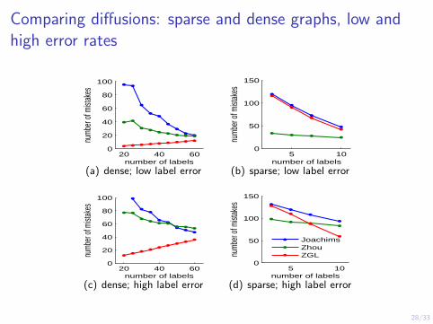
Comparing diffusions: sparse and dense graphs, low andhigh error rates

20 40 600

20

40

60

80

100

number of labels

numb

er of

mist

akes

(a) dense; low label error

5 100

50

100

150

number of labels

numb

er of

mist

akes

(b) sparse; low label error

20 40 600

20

40

60

80

100

number of labels

numb

er of

mist

akes

(c) dense; high label error

5 100

50

100

150

number of labels

numb

er of

mist

akes

JoachimsZhouZGL

(d) sparse; high label error

29/33

Case study with toy digits data set

1 1.5 2 2.50

0.1

0.2

0.3

0.4er

ror

rate

σ

0.8

1.2

1.5

1.8

2.1

2.5

ZhouZhou+Push

(e) Varying σ

102

0

0.1

0.2

0.3

0.4

erro

r ra

te

nearest neighbors

5 10 25 50 100

150

200

250

ZhouZhou+Push

(f) Varying nearest neighbors

Performance of the diffusions while varying the density by changing (a) σor (b) varying r in the nearest neighbor construction. In both cases,making the graph “denser” results in worse performance.

30/33

Densifying sparse graphs with matrix polynomials

Do it the usual way:

I Vary the kernel density width parameter σ.

I Convert the weighted graph into a highly sparse unweightedgraph through a nearest neighbor construction.

Do it by coundint paths of different lengths:

I Run the Ak construction: given a graph with adjacency matrixA, the graph Ak counts the number of paths of length up to kbetween pairs of nodes:

Ak =k∑`=1

A`.

I That is, oversparsify, compute Ak for k = 2, 3, 4, and then donearest neighbor construction.

(BTW, this is essentially what local spectral methods do.)

31/33

Error rates on densified sparse graphsNeighs. Avg. Deg Neighs. k Avg. Deg

13 19.0 3 2 18.128 40.5 5 2 39.237 53.3 3 3 52.373 104.4 10 2 103.897 138.2 3 4 127.1

Table: Paired sets of parameters that give us the same non-zeros in anearest neighbor graph and a densified nearest neighborgraph Ak .

Zhou Zhou w. PushAvg. Deg k = 1 k ≥ 1 k = 1 k ≥ 1

19 0.163 0.114 0.156 0.11741 0.156 0.132 0.158 0.11353 0.183 0.142 0.179 0.136

104 0.193 0.145 0.178 0.144138 0.216 0.102 0.204 0.101

Table: Median error rates show the benefit to densifying a sparse graphwith the Ak construction. Using average degree of 138 outperforms all ofthe nearest neighbor trials from previous figure.

32/33

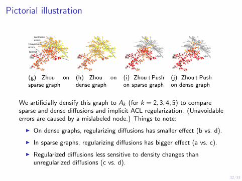
Pictorial illustration

Avoidable errors

Unavoidableerrors

Correct

(g) Zhou onsparse graph

(h) Zhou ondense graph

(i) Zhou+Pushon sparse graph

(j) Zhou+Pushon dense graph

We artificially densify this graph to Ak (for k = 2, 3, 4, 5) to comparesparse and dense diffusions and implicit ACL regularization. (Unavoidableerrors are caused by a mislabeled node.) Things to note:

I On dense graphs, regularizing diffusions has smaller effect (b vs. d).

I In sparse graphs, regularizing diffusions has bigger effect (a vs. c).

I Regularized diffusions less sensitive to density changes thanunregularized diffusions (c vs. d).

33/33

Conclusion

I Many real data graphs are very not nice:I data analysis design decisions are often reasonable but

somewhat arbitraryI “noise” from label errors, node/edge errors, arbitrary decisions

hurt diffusion-bsed algorithms in different ways

I Many preprocessing design decisions make data more nice:I “good” when algorithm users do it—it helps algorithms return

something meaningfulI “bad” when algorithm developers do it—algorithms don’t get

stress-tested on not nice data

I Local and locally-biased spectral algorithms:I have very nice algorithmic and statistical propertiesI can also be used to robustify the graph construction step to

arbitrariness of data preprocessing decisions