Using massively-parallel supercomputers to model stochastic spatial predator-prey systems
Mark Smith*
Department of Physics, UniversiO' ~[ Edinburgh, Edinburgh, U.K.
(Accepted 13 May 1991)
ABSTRACT
Smith, M., 1991. Using massively-parallel supercomputers to model stochastic spatial predator-prey systems. Ecol. Modelling, 58: 347-367.
Massively parallel supercomputers open the door to extensive study of ecological simula- tions that in the past have required prohibitive amounts of computation time. An implementa- tion of a stochastic spatial predator-prey model on such a supercomputer is described. A model that can produce Volterra type oscillations, is extended to study the effectiveness of preferential migration rules for predators and prey. A comparison of various predator migra- tion rules, and results of an initial investigation into the effects produced by mutation of predator migration rates are given.
INTRODUCTION
For over 80 years scientists have been using mathematical techniques to study the dynamics of animal populations (Lotka, 1925; Volterra, 1926). In the recent past concern has been expressed by den Boer (den Boer, 1981) at the reality of 'universal deterministic models'. He showed that, in a heterogeneous environment, dispersion of prey is necessary to ensure the sur- vival of isolated populations. In addition a spatial predator-prey model that includes diffusion can provide a globally stable system from inherently unstable local interactions (Hilborn, 1979). Similar persistence of species (Zeigler, 1977) has also been shown for stochastic spatial models where, in isolated cells, populations would rapidly decay to extinction. Zeigler studies the parameter region that provides global stability for a 100-site world, and
*The author is currently a member of the Department of Statistics at the University of Edin- burgh. Postal address: James Clerk Maxwell Building, King's Buildings, Mayfield Road, Edinburgh.
states that the region is increased for a larger 900-site model. As we strive to increase the reality of ecological models by increasing the size of our mod- el worlds, and by studying longer term effects in these worlds, we are often halted by the limitations of the computer doing the simulations.
Within the spatial model described below, predators and prey are able to migrate to neighbouring locations in a two-dimensional world. Dubois (Dubois, 1975) introduced a non-linear deterministic model of simple predator-prey relations coupled with diffusion to explain observed pat- chiness in plankton populations. However, that work and others (Levin, 1976, Murray, 1975) have found that deterministic patchiness or waves soon decay away to leave a quasi-equilibrium state. The stochastic study detailed here extends diffusion into preferential migration by both species according to a selection of migration rules, and successfully produces dynamic pat- chiness throughout the simulations.
Previous work (Shiyom, 1980) accredited predators with certain levels of mobility and attack ability, in order to study the effects on the spatial pat- terns of a stationary prey. In this paper we introduce some measure of power into the predators' attack ability, and allow the prey species to migrate, potentially according to preferential rules. Besides studying the geographical distributions of the two species during simulations, it was also our intention to compare the effect of different migration rules on the stability of the system, and take a brief look at the effects produced by the mutation of predator migration rates.
S U P E R C O M P U T E R S IN E C O L O G I C A L M O D E L L I N G
These intended extensions to the standard predator-prey model increase computation time dramatically, and the use of a large world would make normal sequential execution prohibitively expensive. In (Onstad, 1988) Onstad predicted that supercomputers would be increasingly used for this type of study since theoretical models cannot be generally accepted if they are not realistic, and realism requires vast amounts of compute-time. There is increasing evidence (Haefner, 1991) that Onstad's prediction is being realised, and that parallel computing technology is a major contributor to this advance. Haefner's review of this subject concentrates upon individual- based models and the various parallel architecture machines that are avail- able, giving some references to current simulation work. In Conrad and Rizki's review of their modelling work (Conrad and Rizki, 1989) there is reg- ular allusion to the short-comings of available computer hardware. As their models became more complex, so the ability to study them in depth was reduced due to computing resources.
M O D E L L I N G STOCHASTIC' SPATIAL P R E D A T O R - P R E Y SY ST E MS 349
Why parallelise?
Almost from the moment of the introduction of the first computer into the research community, scientists have had a desire for ever increasing com- putational power. Improving performance seems to lead inevitably towards new problems that require even more power to solve them. Unfortunately present semi-conductor technology is reaching the absolute limits set by the fundamental laws of physics; electrons can travel through the chip no faster than the speed of light, and the distances they travel must be long enough to overcome quantum uncertainties. We have therefore almost reached the maximum calculation speed possible from a single processor, and the only way left to further increase computational power is to multiply the number of processors being used. This fact is being acknowledged by every major computer manufacturer as they all look toward parallel processing for their future machines (Trew and Wilson, 1991).
The performance gains from using a parallel computer do not, however, come for free. The programmer must put in extra effort to identify potential parallelism within a problem, and then convert this into writing a parallel program for a particular machine. Parallelism does not change the fun- damental nature of the problem solution, it simply provides the means to solve larger problems in shorter times. The rewards provided by parallelisa- tion can therefore be high; in the work covered by this paper, large spatial models that would take days to study using a normal departmental main- frame computer were viewed (via direct high-resolution graphical output) and analysed in a matter of minutes.
The DAP supercomputer
The AMT Distributed Array Processor (DAP-610) is a massively parallel supercomputer containing 4096 processing units* that can perform calcula- tions in parallel. These processors are arranged in a regular 64 x 64 array with optional periodic boundary conditions, producing a mesh of processors that form the surface of a torus, thus avoiding the edge effects introduced by using a finite 2-D grid. The machine can achieve up to twenty million floating point calculations per second and around ten billion logical opera- tions per second. It provides the computing power necessary to study systems that in the past have required excessive computation times.
*The work was originally performed on a DAP-510 in Edinburgh, this machine contained 1024 processing elements.
350 M, SMITH
The DAP is a single instruction multiple data (SIMD) computer. This means that each processor does the same calculations at a particular time, but operates on its own data. There is in addition to the local memory on each processor, an extremely fast transfer of data between processors. Each processor has links to its four neighbours, and data can be transferred through these links at up to 1200 million bytes/s. Therefore, for problems containing many components each of which undergo the same operations, on potentially different data, and involve the transfer of information between these components, the DAP is an ideal simulator. This is exactly the case with the spatial individual-based model studied in this work. Each of the pro- cessing elements is responsible for one location within the model, and makes the necessary calculations for each of the inhabitants of that site. Then in a synchronised step all migrations are carried out by processing elements com- municating migratory numbers with their neighbours.
One of the DAPs strongest features for easing the burden of parallelisation for the programmer, is the fact that it can be programmed in a high-level variant of FORTRAN (Fortran-Plus) that contains implicit functions to handle many of the parallel tasks. In addition the system is hosted by a Sun workstation, allowing file storage and data manipulation to take place within a Unix environment.
T H E P R E D A T O R - P R E Y M O D E L S I N V E S T I G A T E D
The predator-prey models studied in the course of this work were all chosen to make the maximum possible use of the parallel architecture of the DAP supercomputer. The models have a spatial dimension in which each of the processing units in the machine takes responsibility for a section of the system. It is simplest to think of each processor as controlling a field that contains a certain number of each species. There are therefore 4096 locations in each model, arranged on a two-dimensional grid. The periodic boundary conditions applied to the grid give an approximation to an infinite model in that boundary effects are eliminated. However, cyclic effects are introduced, all be it on a large scale. The model can therefore be likened to a stochastic Turing system (Turing, 1952) in two dimensions.
As the simulation evolves, calculations are made to decide whether an in- dividual animal will migrate, die or reproduce. This is therefore an individual-based model, in some ways similar to those studied by Zeigler and Conrad, however, on a much larger scale both spatially and temporally. At the end of each time-step the numbers of migrating animals are transferred between processors. A graphical display of the populations inhabiting each location is continuously produced. Total populations are recorded separately.
M O D E L L I N G S T O C H A S T I C SPATIAL P R E D A T O R - P R E Y S Y S T E M S 351
Lotka- Volterra and Volterra oscillations
The work of Lotka and Volterra in the early 1920s (Lotka, 1925; Volterra, 1926) laid much of the foundation for present models of population dynamics. The coupled differential equations they developed produce now- famous deterministic population oscillations. The initial objective of this work was to recreate these oscillations in a stochastic model that tracks all animals individually, deciding whether birth, death or migration will take place by comparing uniformly randomly generated numbers to assigned pro- babilities.
The model owes much to the work of Wolff (1989) in its design and parameter values. It is based upon predators having two states - - hungo' or satisfied, the state assigned depends on whether the predator has or has not made a kill in the previous time-step. The state of a predator determines the probability that it may reproduce or die. Additionally there are probabilities to determine whether members of either species will migrate to another cell. Table 1 lists all the probabilities relating to a single time-step; these remain invariant throughout all the simulations. These parameter values were those used by Wolff in his work, and have been chosen since they produce the desired Predator-Prey oscillations for a random movement model.
For each individual simulation there were two more important parameters, which were varied between simulations as part of the study. The first of these parameters was the carrying capaci o, of a location (field) with respect to the prey species. The Lotka-Volterra oscillations are produced without this factor, and can not be stochastically modelled without an ex- ponential explosion in the populations. However when carrying capacity was introduced by Volterra (1931) the resulting Volterra Oscillations do lend
themselves to stochastic modelling. The carrying capacity was the maximum prey population that a location could support in the absence of predators. This was therefore a limiting factor to prevent prey populations rising ex- ponentially. The prey birth routine reduces the probability of reproduction as the prey population rises, so that the probability will reach zero as the population reaches the carrying capacity (Equation 1).
Pr(birth) = bp X (1 - (Cell Population/K)) (1)
The second parameter was called the predator-power. It measured the average hunting ability of a predator. The predator-power was the probabil- ity that a predator would catch a particular prey that was in the same loca- tion during a single time-step. Once a prey is caught, the predator becomes satisfied and stops hunting; should the prey escape, the predator will attempt to catch another prey inhabitant of the field, should one exist. Typical ranges of values for these two parameters are given in Table 2.
In order to mimic the non-spatial Volterra model with this spatial stochastic model there was a complete remix of animals at each time-step. In effect animals were allowed to migrate to any randomly chosen location in the 'world'. Although unrealistic when compared to nature, this simulation is intended to remove the spatial aspects of the system, and thus act as a con- trol to test the suitability of the model. The reshuffle of animals is im- plemented such that the field populations lie on a Poisson distribution and, using the probabilities given above, produces oscillations.
Preferential migration simulations
The model was then extended to introduce rules for the preferential migra- tion of the predators and prey. Random infinite migration was replaced with migration into one of the four neighbouring locations (North, South, East or West). The choice of cell into which to migrate was made either complete- ly randomly or according to certain rules. Predators and prey were therefore divided into two subclasses, random-movers and rule-movers.
M O D E L L I N G S T O C H A S T I C SPATIAL P R E D A T O R - P R E Y SY ST E MS 353
In each simulation the initial populations of predators and prey contained just 2-3% of rule-moving animals, the rest being random-movers. There was no method of inter-breeding between the two subclasses in each species, therefore random-movers would always give birth to like animals, as would rule-movers. In addition the preferential migration had no effect on a predator's hunting abilities, or a prey's escaping abilities, once they inhabited the same field. We discuss below the relative success of various preferential migration rules in terms of the growth or decline of the rule-moving propor- tion of the populations.
Mutation simulations
Since the model had been designed to follow individual members of each species, it was not a difficult task to allow certain individual attributes of the animals to vary. There could also be small changes made to these attributes during the course of a simulation, for example a mutation in a parameter value as it was passed from one generation to the next. The parameter chosen to be varied in this initial investigation was the migration probability of the predator species.
The predators were divided into ten groups each with a different probabil- ity of migration (in equal intervals from 0.1 to 1.0). If this were the only adaption made to the model, it would be expected that the population would simply swing towards the faster (more frequent) movers, since their addition- al speed will allow them to cover more fields and therefore increase their probability of finding food. There was therefore a relation introduced be- tween the migration probability of a predator and its reproduction capabili- ty. As the predator used more resources to migrate, it had less left to use for reproduction.
Allowing a small percentage of predators to pass on a mutated migration probability (and therefore reproduction probability) to their offspring, made possible the study of the formation~of distributions of the predator popula- tion between the various classes of animal.
RESULTS
Volterra oscillations
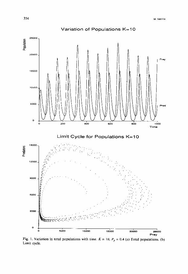
These simulations were run over 1500 timesteps using initial populations of 10 000 prey and 6000 predators. These populations were randomly scat- tered throughout the world using a Poisson distribution. Figure 1 shows the variation with time of the total populations of predators and prey using
3 5 4 M. SMITH
V a r i a t i o n of P o p u l a t i o n s K = I O
2 0 0 0 0
2 5 0 0 0 _
1 5 0 0 0
IOuO0
5 0 0 0
Prey
P r e d
0
0
t 2 0 0 4 0 0 6 0 0 8 0 0 1 0 0 0
T i m e
Limit C y c l e for P o p u l a t i o n s K = I O
O-
1 5 0 0 0 _
1 2 0 0 0
0 0 0 0
6 0 0 0
3 0 0 0
• = " . : . . . ° . •
• . . . . •
- ' i - . - . " " " : . . - " " "
~:-.:_ • . ,
s'.-'.
~,.• •
-?.
i ~ . -
~ - .
!..-
. ° .
i i . i ::: ' i•i ~.:-.'- . . . . . . . . . . ". •:.== . , t - - " " . . . . : ' : " . " - .
~..~'~'- .7-"- ." z7 ~:~ - ' . : - - " "" o
• • . . .
.
- , . • - .
• . . . .
• - - :-
. - . . ' . " • . - "
• • : • • • • • • : • . •
" • . " . .
5 0 0 0 1 0 0 0 0 1 5 0 0 0 20( )00 2 5 0 0 0
P r e y
Fig. 1. Var ia t ion in total populat ions wi th time. K = 1U, Pp = 0.4 (a) Tota l populat ions. (b) L i m i t c y c l e •
MODELLING STOCHASTIC SPATIAL PREDATOR-PREY SYSTEMS 3 5 5
K = 10 and Pp = 0.4. The Volterra oscillations are quite clear. Figure 1 also shows the corresponding limit cycle for these oscillations.
These oscillations were encouraging, showing that the simulation produces results that can be used as a solid base for further investigations. Increasing each field's carrying capacity to K = 15 produced more regular and larger oscillations in the populations. On many simulations the prey species was forced into extinction after a number of cycles. This is something that cannot be reproduced by deterministic equation models, but requires the demographic stochasticity that this model provides. A similar effect was pro- duced by holding K = 10 and raising Pz, to 0.5. This decreases the chances of prey survival, and therefore when they are small in number, increases the chances of a distribution of predators occurring that can force the prey to extinction.
An alternative phenomenon can be produced by decreasing either K or Pp. A more stable system is now produced, and any initial oscillation damps down to give fairly level populations (Fig. 2).
Var ia t i on of Popu la t i ons K=5
1 0 0 0 0
8000
6OOO
4 0 0 0
P r e y P r e d
2000
0 , , , , ,
0 2 0 0 4 0 0 6 0 0 8 0 0 1 0 0 0
T i m e
Fig. 2. Populations through time for K = 5 and Pp = 0,4.
356 M, SMITH
Preferent&l migration simulations
Following the successful reproduction of typical predator-prey phenome- na using this spatial model, the model was extended to investigate the effects produced by introducing preferential migration rules for both species.
Animals can now move into one of the four neighbouring fields only, whether they are moving preferentially or randomly. Each of the simulations was run over the same time period (1500 time-steps), and used the parameters detailed in Table 1. Initially there was a Poisson distribution of 10 000 random-moving prey and 16 000 random-moving predators, with an addi- tional 200 rule-movers from each species. Throughout all the runs K = 10 and Pp = 0.3.
Foxdelay. In the Foxdelay simulation the migration rule weighted the probability of predator migration towards a neighbouring field by the prey population in that field as a proportion of the total prey population in all four neighbouring fields (Fig. 3). Similarily the rule-moving prey would preferentially migrate towards the neighbouring field with the smallest predator population.
Foxdelay acquired its name from the asynchronous nature of the popula- tion counting and the movement of the species. The migration probabilities used the field populations as they were at the start of the migration routine. However, the prey migrate first, and the predators then migrate with the knowledge of where the prey have already migrated to. Therefore the rule- moving predators had a stronger preferential migration rule than the prey. Figure 4 shows the rise to dominance of the rule-moving animals of both spe- cies as well as the time evolution of the total populations.
TPr=26/49
Pr= ~ ~ 8/49 ¢ Pr= 13/49
Pr=2/49 ;
@ Fig. 3. Preferential predator migration probabilities for Foxdelay.
MODELLING STOCHASTIC SPATIAL PREDATOR-PREY SYSTEMS 357
Propor t ion of Ru le M o v e r s for F o x d e l a y
o :3_
100
80
60
40
20
r
Pred
0 300 600 900 1200 1500 Time
V a r i a t i o n of To ta l
20000
16000
12000
8000 I 4000
0
t ions for F o x d e l a y
90 300 600 1 0 0
I Prey
Pred
I ~oo "Nine Fig. 4. Foxdelay: (a) Proportion of preferential migrators in populations, (b) Total populations.
358 MSMITH
It can be seen that the rule-movers of both species rise to dominance to the extent of extinction of the random-movers. The predators reached this state much sooner than the prey. This was probably due to their advantage of migrating second. The graph of total populations shows that the model still produced predator-prey type oscillations. It is interesting to note the in- crease in oscillation size as both species become dominated by rule-movers. This is a phenomenon that occurred with each of the migration rules.
A variety of initial distributions of predators and prey were also in- vestigated with this model. For example, having a random prey distribution and all predators starting in the centre of the world. Alternatively starting with all predators in one section of the world and all prey in another. How- ever no interesting effects were observed with any of the non-random initial distributions since the peculiarity of the distribution was destroyed within one cycle of the oscillation.
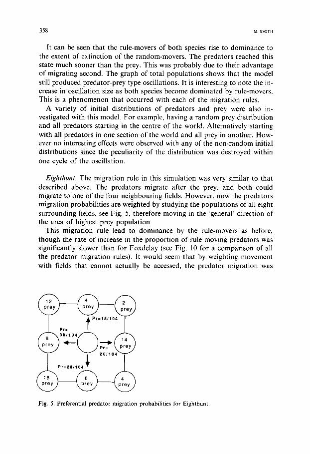
Eighthunt. The migration rule in this simulation was very similar to that described above. The predators migrate after the prey, and both could migrate to one of the four neighbouring fields. However, now the predators migration probabilities are weighted by studying the populations of all eight surrounding fields, see Fig. 5, therefore moving in the 'general' direction of the area of highest prey population.
This migration rule lead to dominance by the rule-movers as before, though the rate of increase in the proportion of rule-moving predators was significantly slower than for Foxdelay (see Fig. 10 for a comparison of all the predator migration rules). It would seem that by weighting movement with fields that cannot actually be accessed, the predator migration was
pr s ~ ~ P r=18/1-~4 ~ ~
Fig. 5. Preferential predator migration probabilities for Eighthunt.
MODELLING STOCHASTIC SPATIAL PREDATOR-PREY SYSTEMS 359
weakened. At the same time, however, the prey rise to dominance was much faster than for Foxdelay. This can be explained by considering that in order to undergo a population boom, a prey species must have resided in an area relatively devoid of predators. This demographic stochasticity allows localis- ed population explosions, as well as the survival of small populations. The weakening of the predator hunting rule probably allowed the formation of more of these predator-free areas, therefore giving the small number of rule- moving prey the opportunity to dominate more rapidly.
Limitfox. The Limitfox migration rule was identical to that of Foxdelay, however the rule moving predators were restricted from dominating com- pletely by the introduction of a 5% probability that a rule-moving predator would produce offspring that were random-movers. This slight weakening of predator power allowed the rule-moving prey to dominate slightly faster than for Foxdelay (for the same reasons as given in the Eighthunt section), and the rule-moving predator domination, as well as being limited to around 85% of the total population (the mutation was one-way only), was not so swiftly achieved. It is also interesting to note that the oscillations in total populations were not as severe as for Foxdelay; Fig. 10 compares the oscilla- tion size of all the migration rules.
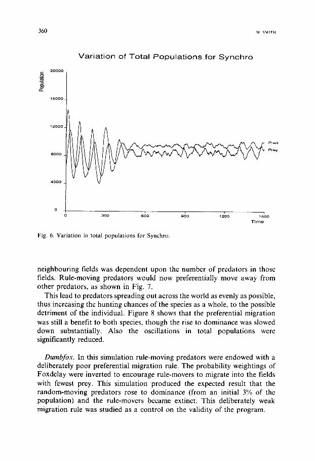
Synchro. As the name suggests, this migration rule had synchronised movement of predators and prey. The Foxdelay probability weighting was used (Fig. 3), but both the predators and prey preferentially migrated using their knowledge of field populations at the end of the previous time-step; the predators therefore have no knowledge of present prey populations, as they do for Foxdelay. This removed the predator advantage described in the Fox- delay Section and produced a significantly weaker preferential migration rule for the predators. That for the prey remained unchanged. The rise to dominance of the rule-moving prey was greatly accelerated, and although in- itially fast the rise to dominance of the rule-moving predators took far longer than for previous rules.
The most interesting result of this simulation can be seen in Fig. 6. The oscillations in the total populations disappear almost completely once both predators and prey were almost all rule-movers. The resulting system was therefore far more stable than for the previous 'stronger' preferential migra- tion rules. Where stability is a measure of the movement, away from an equi- librium population, that occurs for each oscillation. This stability may be local for the particular simulation, and a very large perturbation could throw the system into unstable behavior.
Shyfox. This migration rule had a very different basis for the predator migration. The weighting given to the probability of migration into
360 m SMITH
Var ia t i on of To ta l P o p u l a t i o n s for S y n c h r o
a_
2 0 0 0 0
1 6 0 0 0
1 2 0 0 0
8 0 0 0
4 0 0 0
0
0 , , , , ,
3 o o s o o g o 0 120o 1 5 0 0
T i m e
P r e d
Prey
Fig. 6. Variation in total populations for Synchro.
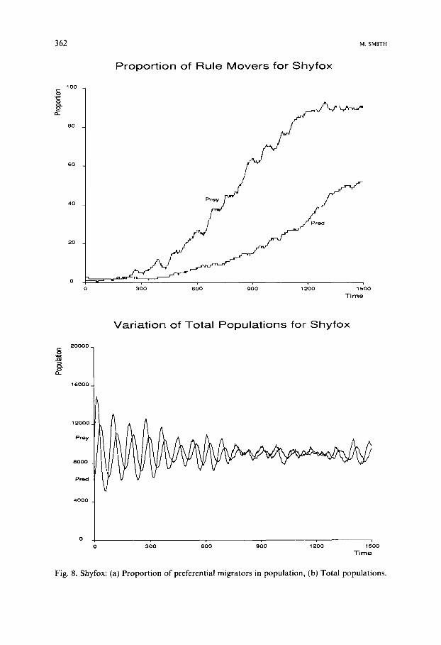
neighbouring fields was dependent upon the number of predators in those fields. Rule-moving predators would now preferentially move away from other predators, as shown in Fig. 7.
This lead to predators spreading out across the world as evenly as possible, thus increasing the hunting chances of the species as a whole, to the possible detriment of the individual. Figure 8 shows that the preferential migration was still a benefit to both species, though the rise to dominance was slowed down substantially. Also the oscillations in total populations were significantly reduced.
Dumbfox. In this simulation rule-moving predators were endowed with a deliberately poor preferential migration rule. The probability weightings of Foxdelay were inverted to encourage rule-movers to migrate into the fields with fewest prey. This simulation produced the expected result that the random-moving predators rose to dominance (from an initial 3% of the population) and the rule-movers became extinct. This deliberately weak migration rule was studied as a control on the validity of the program.
MODELLING STOCHASTIC SPATIAL PREDATOR-PREY SYSTEMS 361
t Pr=20/90 Pr=
Pr=24/90 ~ 28/90
Fig. 7. Probability weighting for Shyfox preferential predator migration.
M u t a t i o n s i m u l a t i o n s
The model was adapted to allow ten varieties of rule-moving predator. These differed in the probability that they would migrate in any one time- step, the probability values were equally spaced from 0.1 to 1.0. In order to prevent faster migrating predators from dominating, the predator reproduc- tion rate was adjusted as well as the migration rate. There was a 0.05 adjust- ment in reproduction probability for every 0.1 change away from the median migration probability (Equation 2).
Pr(birth) = b,. - 0.05 × (/z - 0.5) (2)
Mutation was included in the model by allowing a 2% chance that a reproducing predator would give birth to offspring with a migration probab- ility differing by ± 0.1, and therefore a reproduction probability differing by ± 0.05. This mutation allowed dynamic formation of a distribution of populations of the types of predator. A typical example of such a distribution is shown in Fig. 9. Using a consistent set of simulation parameters, this same distribution was reached from a wide variety of initial distributions, from the two extremes of all fast or all slow predators, and through many intermediate distributions. The distribution is critically dependent upon the simulation parameters used, and also upon the chosen inter-relation between migration and reproduction. There is vast scope to investigate the distributions produc- ed by stochastic models for other inter-relations between predator and prey attributes.
362 M. SMiTH
100 g
" e
80
60
4 0
20
0
P r o p o r t i o n o f R u l e M o v e r s fo r S h y f o x
P r e y
m =
, , . , ,
3 0 0 6 0 0 g o 0 1200 1 5 0 0
T i m e
V a r i a t i o n o f T o t a l P o p u l a t i o n s for S h y f o x
2 0 0 0 0
o_
1 6 0 0 0
1 2 0 0 0
P r e y
8 0 0 0
P r e d
4 0 0 0
f
o 3 0 0 8 0 0 ~ o o ~ 2 0 0 1 5 o o
T i m e
Fig. 8. Shyfox: (a) Proportion of preferential migrators in population, (b) Total populations.
M O D E L L I N G STOCHASTIC SPATIAL P R E D A T O R - P R E Y SYSTEMS
Population
363
H ' I v
Migration Rate
Fig. 9. Population distribution of predator varieties.
CONCLUSION
The results produced by the investigations into various preferential migra- tion rules are summarised in Table 3. These cover a single set of parameter values, no study of the effects produced by varying these parameters was un- dertaken. There is a possibility that some of the effects observed could be parameter-dependent, rather than model-dependent. However, this in- vestigation has centered around investigating the effects of preferential migration on a model known to exhibit predator-prey oscillations. The gra- dient values given are a measure of the strength of the preferential migration rules, in that they are a measure of the speed of the rise to dominance of each of the species. The amplitude of the population oscillations is taken as a mea- sure of the instability of the global system, and is measured from when both populations are dominated by rule-movers.
TABLE 3
Summary of results from preferential migration simulations
Name Pred. gradient Oscillation amp. Prey gradient
Figure 10 shows the relationship between the strength of the preferential migration rules and the stability of the system. Other work (Hilborn, 1979; Zeigler, 1977) has shown that both deterministic and stochastic spatial models can bring stable equilibrium to a system. The results given here show that for very large systems, with periodic boundary conditions used to simulate an infinite world, an individual based stochastic model can run for very long time periods without nearing extinction. However the model still exhibits constant population dynamics, both in terms of oscillations in global populations, as well as dynamic patchiness. In addition, the results show this persistence for a range of predator hunting strategies, and provide some idea of how such strategies affect the stability of the global population.
There appears, even from the few rules investigated, a clear relationship between the strength of the predator hunting rule and the stability of the predator-prey system as a whole. The greater the strength of the predators, the more unstable the system. This suggests that the 'selfish' optimisation of individual improvement produces instability that could lead to the extinction of both the species in the system.
Figure 11 shows the relationship between the success of the rule-moving predators and prey for each predator migration rule. For both species the success of the rule-movers is measured as the gradient of the increase in the proportion of rule-movers in the population. The prey migration rule is iden- tical for each of the different predator migration rules. It can be seen from the graph that for each of the predator rules where the predators are 'chas- ing' prey, the rule-moving prey dominate the prey population faster as the
Oscillation Amplltude(xlO00)
L - E
F =foxdelay
L = l imi t fox
C =synchro
S C E =eighthunt
S =shyfox
I I I I I I l i d 0.1 0.2 0.3 Preda to r
Gradient
Fig. 10. Comparison of the strength and stability of the predator migration rules.
M O D E L L I N G S T O C H A S T I C SPATIAL P R E D A T O R - P R E Y S Y S T E M S 365
P r e y
0.3
0.2
0.1
C
L =lirnitfox
C =synchro
E =eighthunt
S =shyfox
F =foxdelay
E L S F
I i i L i 1 0.1 0.2 0.3 P r e d a t o r
Fig. 11. Comparison of rates of domination of rule-movers.
predator rule weakens. The 'weakness' of the predators seems to give the rule-moving prey more chance to gain rapid control and dominate.
The Shyfox migration rule, where predators attempt to spread themselves evenly across the world+ does not fit into this scheme. This rule may be weak for predators, but it also restricts the rule-moving prey from rapid dominance. This rule produces a very stable system+ where neither species ever acquires a population dense enough to start a population explosion. This seems to suggest that the Shyfox rule is the best to use should global stability and species survival be the major concerns.
The mutation simulations show that introducing mutation into the model, along with some rules defining the inter-relations between predator at- tributes, produces specific distributions of predator types through stochastic methods. There is much room for further study in this area: allowing other attributes to take on a range of values (and mutate within this range) opens the door to finding optimal survival characteristics for members of both spe- cies within complex predator-prey models.
Ecological implications
The ability to simulate large spatial systems in short time periods is of great interest to all ecosystem modellers. There is a constant demand for more accurate models of the real world in order to confirm our theories on animal behavior. The patchiness observed in this 2-D model is somewhat similar to that seen in deterministic models of sea life (Dubois, 1975; Levin, 1976), and the population oscillations produced have been a feature of eco- logical modelling since the pioneering days of Lotka and Volterra.
366 M. SMIT.
One of the important features of this model is that it is stochastic in nature, and exhibits persistent dynamics. It has been shown (Murray, 1975) that deterministic realisations of a spatial Volterra system have no permanent patchiness or wave-like properties since any perturbations decay to equilibri- um. This is contrary to what is observed in the real world. This fundamental difference between the results produced by deterministic and stochastic models is present through a wide range of systems. The deterministic Lotka- Volterra system exhibits damped oscillations, whereas the stochastic version often leads to extinction; the spatial Volterra model gives deterministic decay of perturbations, but stochastic persistence of oscillations (Renshaw, 1991). While it is somewhat risky to place oneself completely within one camp, the merits of stochastic simulations are undeniable. As systems become more complex the cost of performing full stochastic realisations can become pro- hibitive; however, the availability of parallel computers can help to make such work possible.
This availability will be even more important as this work continues into a study of simple evolution. Ever more complex models will be used as muta- tion of parameters is permitted, and thus more calculations are needed for each individual in the system. The case for the use of complex individual based models has been made in the past (Conrad and Rizki, 1989), and this road is potentially lucrative for ecosystem modellers. However there has always been a problem with the limited availability of computation resources, and therefore, until now, very little work has been done on larger model worlds, or on investigating predator migration strategies. This paper has given one method of overcoming practical compute resource problems, and hopefully its results are also of some theoretical interest to ecosystem modellers.
A C K N O W L E D G E M E N T S
This work evolved from a final year's honours project with the Depart- ment of Physics at the University of Edinburgh, supported by a Civil Service bursary for science studies. I gratefully acknowledge the support of Prof. Stuart Pawley and Dr. Richard Kenway, as well as the contributions made by many members of the Physics Department Computational Group.
R E F E R E N C E S
den Boer, P.J. , 1981. On the survival of populations in a heterogeneous and variable environ- ment. Oecologia (Bed.), 50: 39-53.
Conrad, M. and Rizki, M., 1989. The artificial world's approach to emergent evolution. Biosystems, 23, 2(3): 247-260.
M O D E L L I N G S T O C H A S T I C SPATIAL P R E D A T O R - P R E Y S Y S T E M S 367
Dubois, D.M., 1975. A model of patchiness for Prey-Predator plankton populations. Ecol. Modelling, 1: 67-80.
Haefner, J.W., 1991. Parallel computers and individual-based models: An overview. In: DeAngelis and Gross (EditorsL Organisms, Populations, and Communities: A Perspective from Individual-Based Models. Springer-Verlag, NY.
Hilborn, R., 1979. Some long-term dynamics of predator-prey models with diffusion. Ecol. Modelling, 6: 23-30.
Levin, S.A. and Segel, L.A., 1976. Hypothesis for origin of plankton patchiness. Nature, 259: 659.
Lotka, A.J., 1925. Elements of Mathematical Biology. Dover, reissued 1956. Murray, J.D., 1975. Non-existence of wave solutions for the class of reaction-diffusion equa-
tions given by the Volterra interacting-population equations with diffusion. J. Theor. Biol., 52: 459-469.
Onstad, D.W., 1988. Population-dynamics theory: the roles of analytical, simulation, and supercomputer models. Ecol. Modelling, 43: 111-124.
Renshaw, E., 1991. Modelling biological populations in space and time. Cambridge Univer- sity Press.
Shiyom, M., 1980. Predation-affected spatial pattern changes in a prey population. Ecol. Modelling, 11: 1-14.
Trew, A.S. and Wilson, G.V., 1991. Past, Present, Parallel: a survey of available parallel com- puting systems. Springer-Verlag, London.
Turing, A.M., 1952. The Chemical Basis of Morphogenesis. Phil. Trans. R. Soc. Lond. Volterra, V., 1926. Fluctuations in the abundance of a species considered mathematically.
Nature, 118: 558-560. Volterra, V., 1931. Lemons sur la Th6orie Math~matique de la Lutte pour la Vie. Paris,
Gauthier-Villars. Wolff, W., 1989. Population Dynamics, In: Computersimulation in der Physik, 20th
Ferienkurs auf lnstitut fur Festkorperforschung, KFA Jfilich, West Germany, 1989. Zeigler, B.P., 1977. Persistence and patchiness of predator-prey systems induced by discrete
event population exchange mechanisms. J. Theor. Biol., 67: 637-713.