Using OLS to Estimate and Test for StructuralChanges in Models with Endogenous Regressors�

Pierre Perrony

Boston University

Yohei Yamamotoz

Hitotsubashi University

August 22, 2011; Revised November 16, 2012

Abstract

We consider the problem of estimating and testing for multiple breaks in a singleequation framework with regressors that are endogenous, i.e., correlated with the errors.We show that even in the presence of endogenous regressors, it is still preferable, inmost cases, to simply estimate the break dates and test for structural change usingthe usual ordinary least-squares (OLS) framework. Except for some knife-edge cases,it delivers estimates of the break dates with higher precision and tests with higherpower compared to those obtained using an IV method. Also, the OLS method avoidspotential weak identi�cation problems caused by weak instruments. To illustrate therelevance of our theoretical results, we consider the stability of the New Keynesianhybrid Phillips curve. IV-based methods only provide weak evidence of instability. Onthe other hand, OLS-based ones strongly indicate a change in 1991:1 and that afterthis date the model loses all explanatory power.

JEL Classi�cation Number: C22.

Keywords: structural change, instrument variables, parameter variations, PhillipsCurve.

�This is a revised version of parts of a paper previously circulated under the title �Estimating and TestingMultiple Structural Changes in Models with Endogenous Regressors�. Perron acknowledges �nancial supportfor this work from the National Science Foundation under Grant SES-0649350. We are grateful to ZhongjunQu and two referees for useful comments.

yDepartment of Economics, Boston University, 270 Bay State Rd., Boston, MA, 02215 (perron@bu.edu).Ph: 617-353-3026, Fax: 617-353-4449.

zDepartment of Economics, Hitotsubashi University, 2-1, Naka, Kunitachi, Tokyo, 186-8601, Japan(yohei.yamamoto@econ.hit-u.ac.jp)

1 Introduction

Both the statistics and econometrics literature contain a vast amount of work on issues

related to structural changes with unknown break dates (see, Perron, 2006, for a detailed

review). For the problem of multiple structural changes, Bai and Perron (1998, 2003) pro-

vided a comprehensive treatment of various issues in the context of multiple structural change

models: consistency of estimates of the break dates, tests for structural changes, con�dence

intervals for the break dates, methods to select the number of breaks and e¢ cient algorithms

to compute the estimates. Perron and Qu (2006) extended the analysis to the case where ar-

bitrary linear restrictions are imposed on the coe¢ cients of the model. In doing so, they also

considerably relaxed the assumptions used in Bai and Perron (1998). Bai, Lumsdaine and

Stock (1998) considered asymptotically valid inference for the estimate of a single break date

in multivariate time series allowing stationary or integrated regressors as well as trends with

estimation carried using a quasi maximum likelihood (QML) procedure. Also, Bai (2000)

considered the consistency, rate of convergence and limiting distribution of estimated break

dates in a segmented stationary VAR model estimated again by QML when the break can

occur in the parameters of the conditional mean, the variance of the error term or both. Qu

and Perron (2007) considered a multivariate system estimated by quasi maximum likelihood

which provides methods to estimate models with structural changes in both the regression

coe¢ cients and the covariance matrix of the errors. Kejriwal and Perron (2009, 2010) provide

a comprehensive treatment of issue related to testing and inference with multiple structural

changes in a single equation cointegrated model. Zhou and Perron (2007) considered the

problems of testing jointly for changes in regression coe¢ cients and variance of the errors.

More recent work considered the case of a single equation with regressors that are endoge-

nous, i.e., correlated with the errors. Perron and Yamamoto (2012) provide a very simple

proof of the consistency and limit distributions of the estimates of the break dates by show-

ing that using generated regressors, the projection of the regressors of the space spanned

by the instruments, to account for potential endogeneity implies that all the assumptions of

Perron and Qu (2006) (or those of Bai and Perron, 1998) obtained with original regressors

contemporaneously uncorrelated with the errors, are satis�ed. Hence, the results of Bai and

Perron (1998) carry through, though care must be exercised when the reduced form contains

breaks not common to those of the structural form. For an earlier, more elaborate though

less comprehensive treatment, see also Hall et al. (2012) and Boldea et al. (2012).

In this paper, we show that even in the presence of endogenous regressors, in general it

1

is still preferable to simply estimate the break dates and test for structural change using the

usual ordinary least-squares (OLS) framework. The idea is simple yet compelling. First,

except for a knife-edge case, changes in the true parameters of the model imply a change

in the probability limits of the OLS parameter estimates, which is equivalent in the leading

case of regressors and errors that have a homogenous distribution across segments. Second,

one can reformulate the model with those probability limits as the basic parameters in

a way that the regressors and errors are contemporaneously uncorrelated. We are then

back to the framework of Bai and Perron (1998) or Perron and Qu (2006) and we can use

their results directly to obtain the relevant limit distributions. More importantly, the OLS

framework involves the original regressors while the IV framework involves as regressors the

projection of these original regressors on the space spanned by the instruments. This implies

that the generated regressors in the IV procedure have less quadratic variation than the

original regressors. Hence, in most cases, a given change in the true parameters will cause

a larger change in the conditional mean of the dependent variable in the OLS framework

compared to the corresponding change in an IV framework. Accordingly, using OLS delivers

consistent estimates of the break fractions and tests with the usual limit distributions and

also improves on the e¢ ciency of the estimates and the power of the tests in most cases.

This is shown theoretically and also via simulations. Also, the OLS method avoids potential

weak identi�cation problems inherent when using IV methods. Some care must, however, be

exercised. Upon a rejection, one should verify that the change in the probability limit of the

OLS parameter estimates is not due to a change in the bias term and carefully assess the

values of the changes in the structural parameters and the bias terms. In most applications,

there will be no change in the bias but given the possibility that it can occur one should

indeed be careful to assess the source of the rejection. This is easily done since after obtaining

the OLS-based estimates of the break dates one would estimate the structural model based

on such estimates. The relevant quantities needed to compute the change in bias across

segments are then directly available.

To illustrate the relevance of our theoretical results, we consider the stability of the New

Keynesian hybrid Phillips curve as put forward by Gali and Gertler (1999). The results show

that IV-based methods only provide weak evidence of structural instability. On the other

hand, an OLS-based sup-Wald test for one break is highly signi�cant, with 1991:1 as the

estimate of the break date (with a very tight con�dence interval (1990:4 to 1991:2)). The

higher discriminatory power of OLS-based methods over IV-based ones occurs despite the

fact that the instruments are highly correlated with future in�ation. The estimates for the

2

period 1960:1-1991:1 are close to the full sample estimates reported earlier and support Gali

and Gertler�s (1999) conclusion. On the other hand, the estimates for the period 1991:2-

1997:4 are all very small and insigni�cantly di¤erent from zero. Hence, the hybrid New

Keynesian Phillips curve speci�cation has lost any explanatory power for in�ation. This

forecast breakdown of the New Keynesian Phillips curve for in�ation is interesting and can

be traced back to the change in the behavior of in�ation (e.g., Stock and Watson, 2007).

The structure of the paper is as follows. Section 2 introduces the model and summarizes

the relevant result about the limit distribution of the estimates of the break dates using

IV procedures. Section 3 shows how using the OLS framework is not only valid but also

preferable in that it delivers estimates of the break dates with higher precision and tests

with higher power. Section 4 substantiates our theoretical results via simulations and shows

their practical importance. Section 5 presents our empirical illustration related to the New

Keynesian hybrid Phillips curve. Section 6 provides brief concluding remarks.

2 The Model and Results about the IV Procedure

Consider a multiple linear regression model with mx breaks occurring at fT x1 ; :::; T xmxg,

y = �X� + u; (1)

where y = (y1; :::; yT )0 is the dependent variable and �X = diag(X1; :::; Xmx+1) is a T by

(mx + 1)p matrix with Xi = (xTxi�1+1; :::; xTxi )0 for i = 1; :::;mx + 1 with the convention

that T0 = 0 and Tmx+1 = T . We denote the true break dates with a 0 superscript, i.e.,�T x01 ; :::; T x0mx

with the associated diagonal partition of �X by �X0 and the true value of the

coe¢ cient vector �0. Note that this framework includes the case of a partial structural

change model by introducing linear restrictions R� = r with R a k by (mx+1)p matrix with

rank k and r a k dimensional vector of constant. It will be useful also to de�ne the break

fractions (�x01 ; :::; �x0mx) = (T x01 =T; :::; T x0mx

=T ) with corresponding estimates (�x

1 ; :::; �x

mx) =

(T x1 =T; :::; Txmx=T ).

We allow for some regressors to be correlated with the errors and assume that there

exists a set of q variables zt that can serve as instruments, and we de�ne the T by q matrix

Z = (z1; :::; zT )0. We consider a reduced form linking Z andX that itself exhibitsmz changes,

so that

X = �Z0�0 + v; (2)

with �Z0 = diag(Z01 ; :::; Z0mz+1), the diagonal partition of Z at the break dates (T

z01 ; :::; T

z0mz)

and �0 = (�01; :::; �0mz+1). Also, v = (v1; :::; vT )

0 is a T by q matrix, which can be cor-

3

related with ut but not with zt. Given estimates (T z1 ; :::; Tzmz) obtained in the usual way

using the method of Bai and Perron (1998, 2003), one can construct the diagonal parti-

tion Z = diag(Z1; :::; Zmz+1), a T by (mz + 1)q matrix with Zl = (zT zl�1+1; :::; zT zl

)0 for

l = 1; :::;mz + 1. Let � be the OLS estimate of the parameter in a regression of X on Z.

The instruments are then X = Z� = diag(X 01; :::; X

0mz+1)

0 where Xl = Zl(Z0lZl)

�1Z 0leXl witheXl = (xT zl�1+1

; :::; xT zl)0, so that its value in regime l is obtained using only data from that

regime. The relevant IV regression is then

y = �X�� + eu; (3)

subject to the restrictions R� = r, where �X� = diag(X1; :::; Xmx+1), a T by (mx+1)p matrix

with Xj = (xTxj�1+1; :::; xTxj )0 for j = 1; :::;mx + 1. Also, eu = (eu1; :::; euT )0 with eut = ut + �t

where �t = (x0t � x0t)�j for T

x0j�1 + 1 � t � T x0j . The estimates of the break dates are then

(T x1 ; :::; Txmx) = arg min

T1;:::;TmxSSRRT (T1; :::; Tmx); (4)

where SSRRT (T1; :::; Tmx) is the sum of square residuals from the restrictedOLS regression (3)

evaluated at the partition fT1; :::; Tmxg. We also de�ne the break fractions (�x01 ; :::; �x0mx) =

(T x01 =T; :::; T x0mx=T ) with corresponding estimates (�

x

1 ; :::; �x

mx) = (T x1 =T; :::; T

xmx=T ).

Let the union of the break dates in the structural and reduced form be denoted by

(T 01 ; :::; T0m) with the corresponding regime indexed by i for i = 1; :::;m. Note that m need

not equal mx+mz if some break dates are common. It will be convenient to state the set of

assumptions used, which will permit us to de�ne the notation to be used throughout. These

are the same used in Perron and Yamamoto (2012) following Perron and Qu (2006).

� Assumption A1: Let wt = (x0t; z0t)0. For each i = 1; :::;m + 1, let �T 0i = (T 0i+1 � T 0i ),

then �1=�T 0i

� T 0i�1+[�T 0i s]Xt=T 0i�1+1

wtw0t !p Q

i(s) �

24 QiXX(s) QiXZ(s)

QiZX(s) QiZZ(s)

35 ;a non-random positive de�nite matrix uniformly in s 2 [0; 1].

� Assumption A2: There exists an n0 > 0 such that for all n > n0; the minimum

eigenvalues of (1=n)PT 0i +n

t=T 0i +1ztz

0t and of (1=n)

PT 0it=T 0i �n

ztz0t are bounded away from zero

(i = 1; :::;m).

� Assumption A3: rank[E(xtz0t)] = p and the matrixPk1

t=k2ztz

0t is invertible for k1� k2 �

�T for some � > 0.

4

�Assumption A4: Let the Lr-norm of a randommatrixA be de�ned by kAkr = (P

i

Pj E jAijj

r)1=r

for r � 1: (Note that kAk is the usual matrix norm or the Euclidean norm of a vector.)

With fFt : t = 1; 2; ::g a sequence of increasing �-�elds, we assume that fztut;Ftg forms aLr-mixingale sequence with r = 2 + " for some " > 0. That is, there exist nonnegative con-

stants fct : t � 1g and f j : j � 0g such that j # 0 as j !1 and for all t � 1 and j � 0;we have: (a) kE(ztutjFt�j)kr � ct j; (b) kztut � E(ztutjFt+j)kr � ct j+1: Also assume (c)

maxt ct � K < 1; (d)P1

j=0 j1+k j < 1; (e) kztk2r < M < 1 and kutk2r < N < 1 for

some K;M;N > 0.

� Assumption A5: fztvt;Ftg also satis�es Assumption A4 and suptjjztz0zjj = Op(log1=2 T ).

� Assumption A6: T 0i = [T�0i ] , where 0 < �01 < ::: < �0m < 1.

� Assumption A7: The minimization problem de�ned by (4) is taken over all possible

partitions such that Ti � Ti�1 � �T for some � > 0.

� Assumption A8: Let �T;i = �0i+1��0i . Assume �T;i = vT�i, for some �i independent of

T where vT > 0 is a scalar satisfying either a) vT is �xed, or b) vT ! 0 and T 1=2�hvT !1for some h 2 (0; 1=2).

� Assumption A9: Let �T 0i = T 0i � T 0i�1, for i = 1; :::;m, and wt = (x0t; z0t)0. Then, as

�T 0i !1, uniformly in s 2 [0; 1]:

1.(�T 0i )�1PT 0i�1+[s�T

0i ]

t=T 0i�1+1wtw

0t !p sQ

i � s

24 QiXX QiXZ

QiZX QiZZ

35 ;2. (�T 0i )

�1PT 0i�1+[s�T0i ]

t=T 0i�1+1eu2t !p se�2i ;

3. (�T 0i )�1PT 0i�1+[s�T

0i ]

t=T 0i�1+1

PT 0i�1+[s�T0i ]

r=T 0i�1+1(zrz

0teureut)0 !p s

iZ eU ;

4. (�T 0i )�1=2PT 0i�1+[s�T

0i ]

t=T 0i�1+1zteut ) Bi

Z eU(s) with BiZ eU(s) a multivariate Gaussian process

on [0; 1] with mean zero and covariance E[BiZ eU(s)Bi

Z eU(r)0] = minfs; rgiZ eU :Perron and Yamamoto (2012) provide a short proof about the consistency, rate of con-

vergence and limit distribution of the estimates of the break dates. These are summarized

in the following Proposition.

Proposition 1 a) Under Assumptions A1-A8: for every � > 0, there exists a C <1, suchthat for all large T , P (jTv2T (�j � �0j)j > C) < � for every j = 1; :::;mx. b) Let j = 1; :::;mx

index the mx break dates of the structural form and let i denote the position of the jth break in

the structural form amongst the m total break dates in both the structural and reduced forms

5

(note that i can range from 1 to m). Also suppose that the ith overall regime corresponds to

regime l in the reduced form and the (i+ 1)th overall regime corresponds to regime l� in the

reduced form. Under Assumptions A1-A9, we have:

(�0jQ

i;lHH�j)

2

�0j

i;l

H eU�j

vT (Txj � T x0j )!d argmax

sV(i;l)H (s);

where V (i;l)H (s) =W

(i)1 (�s)� jsj =2 if s � 0 and

V(i;l)H (s) =

q�iH(�

i;2H =�

i;1H )W

(i)2 (s)� �iH jsj =2 if s > 0;

with W (i)1 and W (i)

2 independent Wiener processes de�ned on [0;1], (�i;1H )2 = �0ii;l

H eU�i=

�0iQ

i;lHH�i, (�

i;2H )

2 = �0i(i+1);l�

H eU �i=�0iQ

(i+1);l�

HH �i and �iH = �

0iQ

(i+1);l�

HH �i=�0iQ

i;lHH�i.

They also show that all results pertaining to the problem of testing the null hypothesis

of no structural change using equation (3) remain the same as in Bai and Perron (1998),

although we do not restate these explicitly.

3 Estimating and testing using OLS estimates

In this section, we show that, in most cases, it is preferable to estimate the break dates using

the standard OLS method rather than an IV procedure even in the presence of endogenous

regressors. The reasons are very simple. Assume for simplicity that the break dates are

known and let QiXX be de�ned in Assumption A1, p limT!1E(Xiu) = �i for i = 1; :::;m+1,

then the probability limit of the OLS estimate � from (1) is given by, under A9,

�� = �0 + p limT!1

( �X 00�X0)

�1 �X 00u = �0 + diag(Q1XX ; :::; Q

m+1XX )

�1(�1; :::; �m+1)0

= �0 + [(Q1XX)�1�1; :::; (Q

m+1XX )

�1�m+1)]0:

Any change in the parameter �0 will imply a change in the limit value of the OLS estimate ��,

except for a knife-edge case such that the change in the bias term (QXX)�1� exactly o¤sets

the change in �0. Hence, one can still identify parameter changes using OLS estimates. The

second feature is the well known inequality jjPZXjj � jjXjj so that using an IV procedureleads to regressors that have less quadratic variation than when using OLS. These facts imply

that the estimates of the break dates will, in general, be less precisely estimated using an

IV procedure. The main cause for this is the fact that a change in the parameter �0 will, in

general, cause a larger change in the conditional mean of the dependent variable in the OLS

framework compared to the corresponding change in an IV regression.

6

To make the above arguments more precise, consider writing the DGP (1) as

y = �X0�0 + P �X0u+ (I � P �X0)u

= �X0[�0 + ( �X 0

0�X0)

�1 �X 00u] + (I � P �X0)u =

�X0��T + u�;

where u� = (I�P �X0)u and ��T = [�

0+( �X 00�X0)

�1 �X 00u] for which �

�T !p �

�. So we can consider

a regression in terms of the population value of the parameters, viz., y = �X0�� + u�. It is

clear that in this framework �X0 is uncorrelated with u� so that the OLS estimate, say ��,

will be consistent for ��. This suggests estimating the break dates by minimizing the sum of

squared residuals from the following regression

y = �X�� + u�: (5)

Then, the estimates of the break dates are (T �1 ; :::; T�m) = argminT1;:::;Tm SSR

�T (T1; :::; Tm),

where SSR�T (T1; :::; Tm) = (y � �X��)0(y � �X��). We then obtain directly from Perron and

Qu (2006) that, under standard conditions, the estimates of the break fractions are consis-

tent and have the same convergence rate as in the usual OLS framework with regressors

contemporaneously uncorrelated with the errors. The limit distribution of the estimates of

the break dates is given in the following proposition.

Proposition 2 Under Assumptions A1�A4 and A6-A9 with A2-A4 and A9 stated with xtinstead of zt or wt, A4 and A9 stated with u�t instead of ut and eut (using the notations ��i ,iXU� and B

iXU� instead of �i;

iZ eU ; and Bi

Z eU), with A8 stated in term of ��i = ��i+1 � ��i

instead of �i = �0i+1 � �0i and ��i 6= 0, we have, for i = 1; :::;m:

(��0i Q

iXX�

�i )2

��0i

iXU��

�i

vT (T�i � T 0i )!d argmax

sV (i)(s)

where V (i)(s) =W(i)1 (�s)� jsj =2 if s � 0 and

V (i)(s) =p�i(�i;2=�i;1)W

(i)2 (s)� �i jsj =2 if s > 0;

with �2i;1 = ��0i

iXU��

�i =�

�0i Q

iXX�

�i , �

2i;2 = �

�0i

i+1XU��

�i =�

�0i Q

i+1XX�

�i , �i = �

�0i Q

i+1XX�

�i =�

�0i Q

iXX�

�i .

The proof of the above result is a simple consequences of the model (5) and Perron and

Qu (2006), hence is omitted. Note that the limit distribution depends on��i = ��i+1���i . But

since the OLS estimates are consistent for �� this quantity can still be consistently estimated.

One can then compare the limit distributions of the estimates of the break dates using OLS

7

or the IV procedure. For simplicity, consider the case where the instruments, regressors

and errors have a constant distribution throughout the sample so the moment matrices do

not change across regimes. Also, suppose that the errors are uncorrelated. Then, the limit

distribution of the break fractions based on the IV procedure, denoted �IV , is given by

�0T;iQHH�T;ie�2i T (�i;IV � �0i )!d argmax

sV(i)H (s);

where V (i)H (s) = W

(i)1 (�s) � jsj =2 if s � 0, V (i)

H (s) = (�i;2H =�i;1H )W

(i)2 (s) � jsj =2 if s > 0

with (�i;1H )2 = �0

iiH eU�i=�

0iQHH�i, (�

i;2H )

2 = �0ii+1

H eU�i=�0iQHH�i, and that of the break

fractions based on the OLS procedure, denoted �OLS, is

�0T;iQXX�T;i

��2T (�i;OLS � �0i )!d argmax

s[W (s)� jsj=2];

where ��2 = p limT!1 T�1u�0u� = p limT!1 T

�1(y � �X��)0(y � �X�

�). Note that, even in

this case, the limit distribution of the IV estimate will not be symmetric since �i;2H 6= �i;1Heven with homogenous distributions for the errors and regressors. This makes di¢ cult a

precise comparison of the relative e¢ ciency of the two estimates. Note, however, that the

component that contributes most to the variability of each estimate is the scaling factor on

the left-hand side. Hence, to gain some insights about the relative e¢ ciency of the OLS

and IV estimates, we shall analyze the conditions for which QXX=��2 �QHH=e�2i is positivein the scalar case with one regressor. We then have yt = xt�i + ut and xt = zt� + vt with

QHH = �2�2z, QXX = �2�2z + �2v, e�2i = �2 + 2��i + �2i�2v, �

�2 = �2 � �2(�2�2z + �2v)�1 and

� = E(utvt) such that �2 � �2�2v. Finally,

D � QXXe�2i �QHH��2;

= (�2�2z + �2v)(�2 + 2��i + �2i�

2v)� �2�2z(�

2 � �2(�2�2z + �2v)�1)

= 2�2�2z��i + �2�2z�2i�2v + �2�2v + 2��i�

2v + �2i�

4v + �2�2z�

2(�2�2z + �2v)�1:

We seek su¢ cient conditions such that D � 0. Consider �rst the case where �2v = 0. Then� = 0 so that QHH = QXX = �2�2z and e�2i = ��2 = �2 hold, hence OLS and IV are equivalent

(D = 0). When �2v > 0, we can, without loss of generality, normalize �2v = 1 so that

D = 2�2�2z��i + �2�2z�2i + �2 + 2��i + �2i + �2�2z�

2(�2�2z + 1)�1;

with �2 � �2. First, when �i = 0, QHH � QXX and e�2i = �2 � ��2 = �2��2(�2�2z+�2v)�1 sothat D � 0 and OLS dominates IV. Also, when � = 0, QHH = �2�2z � QXX = �2�2z+�

2v and

8

e�2i = �2 + �2i�2v � ��2 = �2 so that OLS again dominates IV. When �i 6= 0, de�ne a = �2�2z

and xi = �=�i so that D=�2i = 2axi + a + (�2=�2i ) + 2xi + 1 + (a=(a + 1))x

2i . Using the fact

that �2 � �2 a su¢ cient condition for D � 0 is that D� � 0 where

D� = 2axi + a+ x2i + 2xi + 1 + (a=(a+ 1))x2i :

After some algebra we get

a+ 1

2a+ 1D� = x2i + 2

(a+ 1)2

2a+ 1xi +

(a+ 1)2

2a+ 1=

�xi +

a+ 1

2a+ 1

�[xi + a+ 1]

Hence, D� � 0 when xi � �(a+1) or xi � �(a+1=(2a+1)). Using R2 = �2�2z=(�2�2z + �

2v)

these conditions can be expressed as, without the normalization �2v = 1,

R2 � max�1 +

�i�2v

�;�1� �i�

2v

�

�: (6)

Accordingly, OLS dominates IV except for a narrow cone centered around �i�2v=� = �1.Though this case can possibly occur, it is unlikely in practice. For example, if �2v = 1, it

requires that the correlation between the errors and regressors (�) be exactly the negative

of the value of the parameter in the �rst regime (�i). We nevertheless consider the �nite

sample properties of the estimates in that case in Section 4.1.

In summary, it is, in most cases, preferable to estimate the break dates using the simple

OLS-based method. As we shall see below, the loss in e¢ ciency can be especially pronounced

when the instruments are weak as is often the case in applications. Of course, the ultimate

goal is not to get estimates of the break dates per se but of the parameters within each

regime, one should then use an IV regression but conditioning on the estimates of the break

dates obtained using the OLS-based procedure. Their limit distributions will, as usual, be

the same as if the break dates were known since the estimates of the break fractions converge

at a fast enough rate. Using the same logic, we can expect tests for structural change to be

more powerful when based on the OLS regression rather than the IV regression. This will

be investigated through simulations in the next section.

4 Simulation evidence

In this section, we provide simulation evidence to assess the advantages of estimating the

break dates and constructing tests using an OLS regression compared to using an IV regres-

sion. Three scenarios are possible for a change between regimes i and i�1, say: 1) ��i 6= ��i�1

9

and �0i 6= �0i�1; 2) ��i 6= ��i�1 and �

0i = �0i�1; 3) �

�i = ��i�1 and �

0i 6= �0i�1. The �rst is the

most interesting since one can test and form con�dence intervals using either the OLS or IV

method. We discuss this scenario in Section 4.1 with the leading case of regressors that have

a homogenous distribution across segments and with the correlation between regressors and

errors also invariant. In Section 4.2, we consider the case for which either can be changing,

a case not covered by our theory. In Section 4.3, we consider the second scenario. The

third possibility is a knife-edge case that would require a change in the bias term to exactly

o¤set the change in the structural parameters. Even though in practice this case is a remote

possibility, we nevertheless discuss it in Section 4.4.

4.1 Homogenous distributions across segments

The data are generated by yt = xt�t + ut where yt, xt and ut are scalars. We consider, for

simplicity, the case of a single break in the parameter �t occurring at mid-sample, so that

�t =

�c for t 2 [1; T=2] ;�c for t 2 [T=2 + 1; T ] : (7)

First, de�ne the following random variables: ut and vt are i:i:d: N(0; �2u) and i:i:d: N(0; �2v)

with E(utvt) = �; also �t � i:i:d: N(0; �2�) and "t � i:i:d: N(0; �2�), mutually uncorrelated

and also uncorrelated with ut and vt. The regressor xt is kept the same throughout the

speci�cations and is generated by xt = �+ �t + vt and, again for simplicity, we consider the

case of single instrument zt generated by zt =p �t+

p2� "t with 0 � � 2. Note that ut

and vt are correlated so the regressors xt are correlated with the errors ut. The variable �t is

a component common to xt and zt and the parameter controls the extent of the correlation

between the regressors and the instruments. The component "t is added in the generation of

zt to keep the variability of the instrument constant when varying . The data-generating

process can also be expressed as yt = xt�+ut with xt = �+�t+vt and zt =p �t+

p2� "t,

so that the reduced form can be expressed as:

xt = �+ (1=p )zt + (vt �

p(2� )= "t);

= �+ [(1=p )�

p(2� )= p lim

T!1(PT

t=1 zt"t)(PT

t=1 z2t )�1]| {z }

�

zt

+[vt �p(2� )= "t +

p(2� )= p lim

T!1(PT

t=1 zt"t)(PT

t=1 z2t )�1zt]| {z }

et

;

= �+ �zt + et:

10

The error et is then not correlated with zt by construction and it is a valid reduced form

representation. The limit of the �rst stage R2 is R2 ! V ar(�zt)=V ar(xt), where

V ar(�zt) =

�1

� 2p

r2�

Cov(zt; "t)V ar(zt)

�1 +2�

Cov(zt; "t)

2V ar(zt)�2�V ar(zt);

and V ar(xt) = V ar(�t)+V ar(vt). Using Cov(zt; "t) =p2� �2� ; V ar(zt) = 2�

2� , V ar(vt) =

�2v, and V ar(xt) = �2�+�2v, then the limit of theR

2 can be simpli�ed toR2 ! �2�=[2(�2�+�

2v)].

Throughout the simulations is adjusted according to the speci�ed value of R2. Since is

bounded above by 2, the highest possible R2 is �2�=(�2� + �2v). Speci�cally, we set �

2� = 5�

2v

so that the maximum R2 is 0:83. Here, we set �2u = 1; �2v = 1; � = 1 and � = :5. We also

consider a stronger endogeneity parameter � = 1:0. We report results for R2 = :8, :5, :3 and

:1, and c = :25; :5; and 1:0. The sample size is T = 100 and the number of replications is

3000. The results are presented in Figure 1 for the cumulative distribution functions.

The OLS-based estimates are always more precise than the IV-based estimates. The

extent to which the IV-based estimates perform badly increases as R2 decreases, and even

for a value as high as 0:5, which is larger than what can be obtained in most applications, the

IV-based estimates show much higher variability than the OLS-based estimates. In the case

of weak instruments (R2 = :1), the IV-based estimates are not informative. Also, when the

magnitude of change increases, the precision of the OLS-based estimate increases noticeably.

The increase in the precision of the IV-based estimate is, however, not as substantial as c

increases. Hence, even with large breaks, the OLS-based estimates are far superior. The

results are robust when we consider stronger endogeneity with � = 1:0. The simulations

show that it is indeed highly preferable to estimate the break dates using the standard OLS

framework even when the regressors are contemporaneously correlated with the errors.

We also simulated the power of the sup-Wald test for a single break of Quandt (1958,

1960) as developed by Andrews (1993), given by supW = sup[�T ]<Tb<[(1��)T ] [SSRrT �

SSR(Tb)]=[SSR(Tb)=(T � 1)], where SSRrT is the restricted sum of squared residuals from aregression assuming no break, and SSR(Tb) is the sum of squared residuals when allowing

for a break at date Tb. The trimming parameter is set to � = :15 and we report results for

tests with a 5% nominal size. We also considered the UDmax test of Bai and Perron (1998),

for which there is no need to pre-specify the number of breaks. The results were qualitatively

similar and are not reported. To get the power functions, we varied c between 0 and :5. The

results, presented in Figure 2, show that the OLS-based test has the highest power. The

power of the IV-based test is noticeably inferior and decreases as the instrument gets more

weakly correlated with the regressor. The results are again robust to the stronger endogeneity

11

case. Hence, testing should also be performed using the usual OLS-based methods.

4.1.1 The case when IV dominates OLS

As argued in Section 3, there is a region of the parameter space for which IV may dominate

OLS in large samples. It is given by (6) and depicted in Figure 3 and corresponds to a

narrow cone around ��2v=� = �1. It remains to be seen whether using OLS in such casesleads to noticeably inferior estimates in �nite samples. To that e¤ect, we report simulations

setting yt = xt�i + ut, xt = zt� + vt then choose parameter values �i�2v=� = �1 to maximizethe chances that IV is superior. Again, we consider a single break and we use the following

parameter values: �1 = 1, � = (R2=(1 � R2))1=2, �z = � = �v = 1 and � = �1 so that�1�

2v=� = �1 is satis�ed. The sample size is T = 100, and the parameter � has one time

break at mid-sample such that �1 = 1 for t � 50 and �2 = 0:5 afterwards. Again 3,000

replications are used to construct the cdf of the break date estimates for four di¤erent values

of the �rst stage R2. These are reported in Figure 4. They show that indeed IV can

dominate OLS if the �rst stage R2 is high (R2 = 0:5). The di¤erences are, however, small.

When the R2 is smaller, OLS dominates IV and with weak instruments the IV estimate is

uninformative, as expected. Note also the pronounced skewness of the distribution of the

IV estimate. We tried di¤erent parameter values within the set de�ned by Figure 3 and

the results were qualitatively similar. In particular, slight deviations from values satisfying

��2v=� = �1 lead to having OLS-based estimates be more precise than IV-based ones. Thisis important for two reasons. First, it shows the relevance and adequacy of our large sample

approximation to obtain su¢ cient conditions for IV to be superior to OLS. Second, it shows

how restricted, indeed unlikely, is the set of parameters for which IV dominates OLS. Hence,

these results suggest that the cost in �nite samples of using OLS when IV is superior to OLS

using large sample arguments is small, especially compared to the substantial gains of using

OLS in most of the parameter space, as shown above.

4.2 Non-homogenous segments : Scenario 1

We now consider the case for which the distribution of the regressors and the correlation

between the regressors and errors can vary across segments so that the change in the pseudo

limit values ��i = ��i+1 � ��i need not equal the change in the true population values �i =

�0i+1� �0i . Given the nature of the limit distributions stated in Propositions 1-2, it is di¢ cultto provide theoretical results; hence, we resort to simulations. The data generating process

is similar to the one used in the previous section except that we allow some key parameters

12

to change across regimes. More speci�cally, we now have xt = �t + �t + vt, vt � i:i:d:

N(0; �2tv), �t � i:i:d: N(0; �2t�) and E(utvt) = �t. We consider three cases: 1) a change in

QXX induced by a change in the variance of the regressor such that �2tv = �21v for t 2 [1; T=2]and �2tv = �22v for t 2 [T=2 + 1; T ]; 2) a change in the correlation between the regressor andthe errors such that �t = �1 for t 2 [1; T=2] and �t = �2 for t 2 [T=2 + 1; T ]; 3) a changein QXX induced by a change in the mean of the regressor such that �t = �1 for t 2 [1; T=2]and �t = �2 for t 2 [T=2 + 1; T ]. The other speci�cations are the same. Throughout thesimulations, we again set �2t� = 5�2tv so that R

2 is �xed for the whole sample. Note that

= (12=5)R2 is also �xed. Again, in all cases, the sample size is T = 100, the number of

replications is 3000 and we report results for R2 = :8, :5, :3 and :1. The results reported

are the cumulative distribution functions of the IV and OLS-based estimates. In all cases,

we consider changes such that the value of the relevant parameter is smaller or greater in

the �rst regime compared to the second, since the distributions are not symmetric for equal

changes occurring in the two segments. The change in the parameter � is given by (7) with

c = 0:25. We use �2u = 1; �2v = 1; �

2� = 5�

2v; � = 0:5, and � = 1 unless otherwise stated.

Consider �rst case (1) with a smaller variance of the regressor in the �rst regime so that

�22v = 1 and �21v = a with a = 0:8, 0:5 and 0:25. The results are presented in Figure 5 (left

column). Here ��1 is greater in absolute value than �1, so we can expect an increase in

the e¢ ciency of the OLS-based estimate of the break date. When comparing with the base

case in Figure 1, this is indeed the case and more so as a decreases. The results in Figure

5 (right column) pertain to the case of a smaller variance in the second regime so that ��1

is smaller in absolute value than �1. The speci�cations used are �21v = 1 and �22v = b with

b = 0:8, 0:5 and 0:25. One can see a reduction in the e¢ ciency of the OLS-based estimate.

It nevertheless remains more e¢ cient than the IV-based estimate and again more so as the

extent of the correlation between the regressor and instrument decreases.

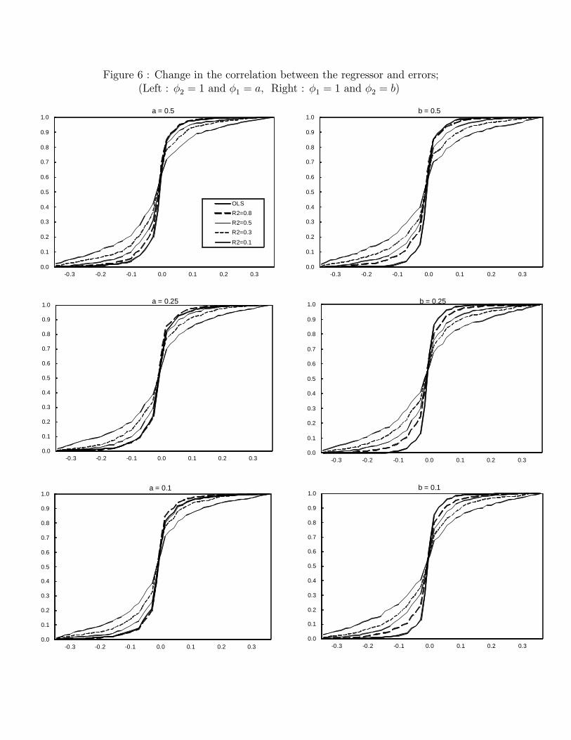
Consider now a change in the correlation between the errors and the regressors across

regimes. The �rst case is one for which the correlation is smaller in the �rst regime given

by �2 = 1 and �1 = a = 0:5, 0:25 and 0:1, for which ��1 is smaller in absolute value than

�1. As depicted in Figure 6 (left column), this translates into a reduction in the precision

of the OLS-based estimate of the break date. We have some instances for which the IV-

based estimate is marginally more precise than the OLS-based one. This, however, requires

a very high correlation between the regressor and instrument and a very large change in the

correlation between the regressor and the errors. The results with a correlation higher in

the �rst regime are presented in Figure 6 (right column) for the speci�cations �1 = 1 and

13

�2 = b = 0:5, 0:25 and 0:1. Here ��1 is greater in absolute value than �1 and the results

show that in all cases the OLS-based estimate is more precise than the IV-based one.

The last case considered has the mean of the regressor changing across regimes. Figure

7 (left column) presents the results when the mean is higher in the �rst regime, speci�ed

by �2 = 1 and �1 = a = 1:5, 2:0 and 5:0. In this case, ��1 is smaller in absolute value

than �1. The OLS-based estimate nevertheless remains more e¢ cient unless the change in

mean is very large (a = 5) and the correlation between the regressor and instrument is high,

even then the di¤erences are minor. When the mean of the regressor is higher in the second

regime ��1 is greater in absolute value than �1. The results in Figure 7 (right column) for

the speci�cations �1 = 1 and �2 = b = 1:5, 2:0 and 5:0 show that the OLS-based estimate is

more e¢ cient than the IV-based one and more so as the change in mean increases.

Overall, the simulations presented showed that, in general, the OLS-based estimate is

more precise than the IV-based one even when the distribution of the regressors or the

correlation between the regressors and the errors change across regimes. There are cases

for which this is not true, though with small di¤erences, but they occur for unrealistically

high values of the correlation between the regressors and instruments and very large changes

in either the correlation between the regressors and errors or the means of the regressors.

Hence, for all practical purposes, it is more bene�cial to use an OLS-based method.

4.3 Scenario 2

In the second scenario ��i 6= ��i�1 and �0i = �0i�1, so that there are no changes in the structural

parameters but there is a change in either the marginal distribution of the regressors xt or

in the correlation between these regressors and the errors ut so that the limit value of the

OLS estimates ��i changes. Since there are no changes in the structural parameters, it is

uninformative to compare the relative e¢ ciency of the estimate of the break dates. Hence,

we concentrate on the rejection frequencies of the tests for structural change using the IV

and OLS methods. The presumption is that the IV method would correctly identify no

change, while the OLS method would incorrectly identify a change. We use simulations to

address this issue and discuss afterwards the practical implications.

Consider �rst the case in which the correlation between the regressors and the errors

changes across segments. Note �rst that the limit distribution of the sup-Wald OLS-based

test does not have the stated limit distribution, while the limit distribution of the IV based

test is not a¤ected. Hence, we can expect size-distortions using the OLS-based method.

Though these are minor for the sup-Wald test, we nevertheless also report the rejection

14

frequencies using critical values obtained using the �xed regressors bootstrap method of

Hansen (2000). We use the same data-generating process as in Section 4.2, except that

�t = 1 throughout. We set �2 = 0:5 and vary �1 between �1 and 1. The results presented inTable 1 show the IV-tests to retain an exact size close to 5%, as expected, and the OLS-based

test can have high rejection frequency if the induced change in bias is large. This is also the

case when the bootstrap tests are used.

Consider now the case of a change in the marginal distribution of the regressors, either a

change in the variance and a change in the mean of xt. Consider �rst a change in the variance

of xt. Since the variance change in xt and that in zt (hence, in xt) occur, none of the IV or

OLS-based sup-Wald tests have the same limit distributions. From results in Hansen (2000)

(see also Kejriwal and Perron, 2010, in a related context) the size distortions of the sup-Wald

test are minor in the presence of a change in the mean of the regressors but substantial when

the variance of the errors change. In the IV case, the variance of the errors in the second

stage regression �t = (xt� xt)� also changes with a change in the marginal distribution of theregressors xt. Hence, we also present results using the �xed regressors bootstrap methods

of Hansen (2000) using the heteroskedastic version. To assess the �nite sample rejection

frequencies, we use the same data-generating process as in Section 4.2, except that �t = 1

and we set �22v = 1 while varying �21v between 10 to 0:25. The results are presented in Table

2. They show the OLS-based test to exhibit liberal size distortions when the bias change is

large. The IV-test has better size provided the heteroskedastic bootstrap method is used,

though even then some size-distortions occur with a large change.

The last case is a change in the mean of the regressors xt. Here, again none of the

IV or OLS-based sup-Wald tests have the stated limit distribution that applies when the

distribution of the regressors is homogeneous. This is so for the IV-based method since a

change in the marginal distribution of xt implies a change in the marginal distribution of

xt. If the reduced form is stable, a change in the mean of xt must be associated with a

change in the mean of the instruments and accordingly in the mean of the �tted values

xt. If the reduced form is unstable but the breaks are properly accounted for, the mean of

xt varies by construction. Again, in the IV case, the variance of the errors in the second

stage regression change. Hence, we also present results using the �xed regressors bootstrap

methods of Hansen (2000) using the heteroskedastic version. Given that the reduced form is

unstable, for the IV-based tests we proceed as follows. We �rst estimate the break date in

the reduced form and test whether the change is signi�cant using a sup-Wald test. If it is, the

break is accounted for when estimating the structural model using the full sample method of

15

Perron and Yamamoto (2012). Table 3 reports the rejection frequencies of the tests using the

same DGP as in section 4.2, except again that �t = 1 throughout and �2 = 1 and �1 varying

between 0:1 and 10 (to obtain a range for the bias similar to the previous experiments).

Here, things are quite di¤erent. As expected, the OLS-based test does have high power

if the change in mean is large. The IV-based test using the standard asymptotic critical

values has the correct size if the instrument is very strongly correlated with the regressor

and the change is small. As the instrument gets more weakly correlated, the size of the test

increases rapidly. The rejection frequencies of the IV-based test exceed those of the OLS-

based test when the R2 of the �rst stage regression is small. Intuitively, as the instruments

get weaker, xt gets closer to a white noise process so that the change in xt cannot fully

account for the change in the mean of yt induced by the change in xt without a concurrent

change in either the regression coe¢ cient, the intercept or both, thereby inducing a change

in the parameters. With tests constructed using the heteroskedastic bootstrap, the size

distortions are considerably reduced for the IV-based test, but can remain important when

the correlation between the regressor and the errors is weak. As expected, the OLS-based

tests have high power even when the heteroskedastic bootstrap version is used.

4.4 Scenario 3

The third scenario pertains to a knife-edge case of �0i 6= �0i�1 but ��i = ��i�1 so that the change

in the structural parameters is exactly o¤set by the bias change induced by a change in the

moments of the regressors or in the correlation between the regressors and the errors. This

is arguably a case of lesser practical relevance but we still include a discussion about it for

completeness. We again consider three cases; 1) a change in the variance of the regressor,

2) a change in the correlation between the regressor and the errors, and 3) a change in the

mean of the regressor. We use �2u = 1, �2� = 5�

2v, � = 1, �

2v = 1 and � = 1 unless otherwise

stated. The changes occur at T=2. We present the distributions of the break date estimates

at ��i = ��i�1 (but �0i 6= �0i�1) in the left column of Figure 8. We also provide power functions

of the sup-Wald test with a 5% nominal size using the asymptotic critical values with c

ranging from 0 to 1 in the right column of Figure 8.

For the �rst case, we set the change from �21v = 10 to �22v = 1 (the largest change

considered in Section 4.3). However, even with such a large variance change, the e¤ective

break in the structural parameter is small (c = 0:063). Figure 8 (the top panel in the left

column) shows that the OLS-based estimate is, as expected, not informative. However, the

cumulative distribution functions of the IV-based estimates are also quite �at. What is

16

more instructive is to look at the relative performance of both methods in a neighborhood

of the knife-edge case. To that e¤ect, we computed the power functions for this case with c

ranging from 0 to 1. The results are in the top right panel of Figure 8. Both the OLS and

IV-based tests have important size distortions at c = 0, consistent with the results presented

in Section 4.3 (though these could be reduced using the bootstrap method). The power of

the OLS-based test decreases up to c = 0:063 (when ��i = ��i�1), but it increases rapidly

afterwards. The OLS method can dominate the IV-based one when the instrument is weak.

We next consider the second case with �1 = �1 and �2 = 1. This represents an (unreal-istically) large change that requires the correlations to vary from perfect negative correlation

to perfect positive correlation at mid-sample. Such a large change is needed to have at least

a modest bias change with magnitude 0:286. The distribution of the OLS estimate of the

break date with c = 0:143 (corresponding to ��i = ��i�1) shows that it is uninformative. The

IV estimates are more precise if the correlations between the regressors and the instruments

are strong, however, it becomes less informative as the instruments get weaker. Looking at

the neighborhood around the knife-edge case, the power function of the OLS-based test has

again a U-shape around c = 0:143 but the power quickly increases as c increases.

For the third case, we again need to consider a large change from �1 = 5 to �2 = 1 along

with a maximum correlation between the regressors and the errors. These yield a bias change

of 0:133 so that the knife-edge case occurs at c = 0:067. The results presented in the bottom

left panel of Figure 8 show that the OLS method is, as expected, uninformative but also

that the IV-based estimate is barely superior irrespective of the strength of the instruments.

Looking at the power function around the knife-edge case, the power of the OLS-based test

dominates the IV-based test regardless of the strength of the instruments (power is above

size when c = 0:067 because of distortions arising from the very large mean shift).

4.5 Practical implications

Our analyses showed the OLS-based procedure to outweigh, by possible large margins, the

IV-based procedure when a change in the structural form occurs (more precise estimate

and tests with higher power). There are exceptions but they all apply to so-called knife-

edge cases that arguably are not likely to occur in practice, and even in such cases IV is

only marginally better than OLS. We also discussed how OLS-based methods can spuriously

detect a change in the structural form when none occurs due to possible changes in the

marginal distributions of the regressors or the correlation between the errors and regressors.

These are of clear relevance in practical applications. Should the fact that the OLS-based

17

tests reject the null hypothesis of no change when ��i 6= ��i�1 and �0i = �0i�1 be of a concern

and a reason to abandon it in favor of the IV-based test? The answer is clearly no but with

the caveat that care must be exercised in practice. Upon a rejection, one should verify that

it is not due to a change in the bias term and carefully assess the values of �0i and the bias

terms (QiXX)�1�i. In most applications, there will be no change in the bias but given the

possibility that it can occur one should indeed be careful to assess the source of the rejection.

The price of discarding the OLS-based method in favor of the IV-based one is too high.

First, in most cases the power of the IV-based method is lower and much more so as the

instruments gets weaker, a common feature in applications. Second, as illustrated by the

case with a change in the mean of the regressors the IV-based test can su¤er from serious

size distortions, which are, however, reduced to a great extent using Hansen�s (2000) het-

eroskedastic bootstrap test. Since these are �nite sample problems, one would not be inclined

to question the source of the rejection and would reach the wrong conclusion. The fact that

we could have ��i 6= ��i�1 and �0i = �0i�1 does not invalidate the OLS-based method, it sim-

ply calls for a more careful analysis. This is easily done since after obtaining the estimates

of the break dates one would estimate the structural model based on such estimates. The

relevant quantities needed to compute the change in bias across segments are then directly

available. Given that the residuals from the IV regression are given by eut = ut + (x0t � x0t)�j

for T 0i�1 + 1 � t � T 0i , an estimate of the change in bias from regime (i� 1) to regime i, canbe obtained as

(TiP

t=Ti�1+1

xtx0t)�1

TiPt=Ti�1+1

(xtbeut � xt(x0t � x0t)�i) (8)

�(Ti�1P

t=Ti�2+1

xtx0t)�1

Ti�1Pt=Ti�2+1

(xtbeut � xt(x0t � x0t)�i�1)

where Ti are the estimates of the break dates obtained using the OLS-based method, beut and�i are the estimated residuals and coe¢ cient estimates, respectively, from the estimated IV

regression.

5 Empirical example

To illustrate the relevance of our results, we consider the stability of the New Keynesian

hybrid Phillips curve as put forward by Gali and Gertler (1999). The basic speci�cation is

�t = �+ �t�1 + �xt + �Et�t+1 + ut (9)

18

where �t is the in�ation rate and Et is the expectation operator conditional on information

available at time t. The variable xt is a real determinant of in�ation usually taken as a

measure of real economic activity such as the output gap, though Gali and Gertler (1999)

argue that using a measure of real marginal cost is preferable. The key ingredient is the

component Et�t+1 which makes the Phillips-curve forward looking. The one-period lag of

in�ation is usually introduced on the ground that it improves the �t of the model but can be

rationalized by supposing that a proportion of �rms use backward-looking rules to set prices.

In this speci�cation, one expects � and to be positive and that � is substantially larger

than so that the forward looking component dominates. Also, � is expected to be positive

so that an increase in real activity is associated with an increase in in�ation. As argued by

Gali and Gertler (1999), the estimate of � is usually negative when using the output gap but

is positive, though quite small, when using real marginal cost.

We follow the approach taken by Gali and Gertler (1999) and use basically the same

speci�cations and data. The data was obtained from Andre Kurmann�s website (and used

in Kurmann, 2007). It is for the U.S.A. and quarterly for the period 1960:1-1997:4 as in Gali

and Gertler (1999). The in�ation rate �t is the quarterly change in the GDP de�ator and xtis either 1) labor income share as a proxy of real unit labor cost (nonfarm business unit labor

cost de�ated by the GDP de�ator), or 2) detrended real GDP assuming a quadratic linear

trend as a measure of the output gap. The only di¤erence is that we use as instruments

only one lag of the following variables: in�ation, labor income share, the output gap, the

interest rate spread (10 years US treasury bill rate minus the 3 years bill rate), wage in�ation

(quarterly change in the nonfarm business nominal wage rate) and the commodity price

in�ation (quarterly change in the spot market price index). Using four lags as in Gali and

Gertler (1999) would imply too many instruments so that testing for changes in the reduced

form, needed for the IV-based methods, becomes impossible with the tests having no power.

Gali and Gertler (1999) estimated the model using a non-linear IV procedure given that

their model implies restrictions across the coe¢ cients which are functions of some basic

parameters. We use a linear IV method of estimation. The results are, however, in line with

those of Gali and Gertler (1999) for the full sample speci�cation and doing so does not a¤ect

our conclusions. The parameter estimates for the full sample are presented in Table 4 for

both cases in which xt is speci�ed as the real marginal labor cost or as the output gap. The

results are in close agreement with those of Gali and Gertler (1999). The coe¢ cient � on

future expected in�ation is large and signi�cant and about twice as large as the coe¢ cient

on lagged in�ation, indicating that the forward-looking behavior is dominant. The estimate

19

of � is positive when using the real marginal cost of labor and negative when using the

output gap, though the values are small and insigni�cant. Note also that the instruments

are quite strongly correlated with future in�ation, the R2 of the �rst-stage regression being

0:73. The results are qualitatively similar using four lags of each variables as instruments.

In order to proceed with the IV-based methods, we need to consider the stability of the

reduced form. This is not needed for the OLS-based method as long as tests are constructed

using the �xed regressors bootstrap method of Hansen (2000). The results presented in Table

5 points to the presence of 1 or 2 breaks. Applying the Bai and Perron (1998) sequential

method, the test for one break is signi�cant at the 1% level using the asymptotic critical

values and at the 10% level using the critical values from Hansen�s (2000) bootstrap method.

The test for 2 versus 1 break is again signi�cant at the 1% level using the asymptotic critical

values but not using the boostrap method, a di¤erence possibly due to the large number of

regressors. In the following, we consider both cases with 1 and 2 breaks.

We now turn to the issue of the stability of this hybrid New-Keynesian Phillips curve.

Consider �rst the OLS-based method. When using the labor income share, the test for one

break is signi�cant at the 1% level using the asymptotic critical values and at the 10% level

using the bootstrap ones. The estimate of the break date is at 1991:1 with a very tight

con�dence interval (1990:3 to 1991:3). There is no evidence for the presence of an additional

break. When using the output gap, the test for one break is again signi�cant at the 1%

level using the asymptotic critical values but not signi�cant using the bootstrap ones. The

estimate of the break date is again 1991:1 with an even tighter con�dence interval (1990:4

to 1991:2). There is again no evidence for the presence of a second break.

We now consider the results obtained using IV-based methods. We start with the sub-

sample approach advocated by Hall et al. (2012), which looks at evidence for changes in the

structural form using the sub-samples induced by the estimates of the break dates in the

reduced form. The results in Table 6 show that one cannot �nd any statistically signi�cant

evidence for the presence of a break. This is true whether one considers a single or two

breaks in the reduced form. Things are somewhat di¤erent when using the full-sample

method advocated by Perron and Yamamoto (2012). Consider �rst the case with one break

in the reduced form at date 1980:4. The results are the same using either the labor income

share or the output gap. The test for one break is signi�cant at the 5% level using the

asymptotic critical values but not when using the bootstrap ones. There is no evidence for

the presence of a second break and the estimate of the break date is 1967:2, very di¤erent

from that obtained using the OLS-based method. Overall, the evidence for a break in the

20

structural form is weaker. Consider now the case with two breaks in the reduced form at

dates 1973:1 and 1980:4. When using the labor income share the results are similar to the

case of a single break in the reduced form. The test for one break is barely signi�cant at

the 10% level using the asymptotic critical values and not using the bootstrap ones. The

estimate of the break date is again 1967:2. Things are di¤erent when using the output gap

with results identical to those obtained using the OLS-based method. The test for one break

is signi�cant at the 1% level using the asymptotic critical values but not signi�cant using

the bootstrap ones. The estimate of the break date is again 1991:1 with a tight con�dence

interval (1990:3 to 1991:3). There is again no evidence for the presence of a second break.

It remains to be seen whether this change in 1991:1 is economically signi�cant. To that

e¤ect we estimated the parameters of the model by IV using the same instruments allowing

for a change in all parameters. The estimates are presented in Table 7. They are indeed very

interesting. The estimates for the period 1960:1-1991:1 are close to the full sample estimates

reported earlier and support Gali and Gertler�s (1999) conclusion. On the other hand, the

estimates for the period 1991:2-1997:4 are all very small and insigni�cantly di¤erent from

zero in both cases. Hence, both of these hybrid New Keynesian Phillips curve speci�cations

have lost any explanatory power for in�ation. Again, the results are qualitatively similar

using four lags of each variables in the instrument list.

As discussed above, the full-sample IV-based method pointed to a break in 1967:2 when

considering one break in the reduced form with either the labor income share or the output

gap and also when considering two breaks in the reduced form when using the labor income

share. To see which of 1967:2 or 1991:1 is the more appropriate break date, we present in

Table 8 the parameter estimates of the structural form with a break in 1967:2. The estimates

show no signi�cant di¤erences between the samples 1960:1-1967:2 and 1967:3-1997:4. The

parameter � shows a slight increase that is not signi�cant, while shows an increase (from

negative to positive) when using the labor income share. With one break in the reduced

form, however, it shows an increase when using the output gap. So the results are sensitive

to the exact speci�cation and also not signi�cant as the standard errors are large in both sub-

samples. The changes when considering a break in 1991:1 are economically more important

and statistically signi�cant than those obtained with a break in 1967:2. This reinforces the

conclusion that the OLS-based method provides more reliable results.

Overall, the results point to the following conclusions. With the OLS-based method, the

evidence for a break in the structural form is strong and points to the same break date,

1991:1, whether using the labor income share or the output gap. When using the IV-based

21

methods, things are not as precise. First, the sub-sample approach yields no evidence for

a break in the structural equation. The more powerful full-sample approach suggested by

Perron and Yamamoto (2012) can deliver strong results in line with the OLS-based ones,

as obtained when considering the output gap. But it can also be less powerful as in the

case for which the labor income share is used. Note �nally that the higher discriminatory

power of OLS-based methods over IV-based ones occurs despite the fact that the instruments

are highly correlated with future in�ation. The OLS-based method is also much easier to

implement without the need to worry about changes in the reduced form.

Finally, we need to assess that the rejection is not due to change in the bias term. To that

e¤ect we estimated the change in the bias from (8) with a break in the srtuctural equation in

1991:1. For the case with one break in the reduced form in 1980:4, the estimated value was

0:0388 with the labor income share and 0:0513 with the output gap. For the case with two

breaks in the reduced form in 1973:1 and 1980:4, the estimated value was 0:0107 with the

labor income share and 0:0212 with the output gap. These compare to a change in coe¢ cient

of 1:011 with the labor income share and 1:052 with the output gap. Hence, the change in

the bias is negligible compared to the change in the parameters so that a rejection using the

OLS-based sup-Wald test genuinely re�ects a change in the structural parameters.

This forecast breakdown of the New Keynesian Phillips curve for in�ation is interesting

and can be traced back to the change in the behavior of in�ation. As argued by Stock and

Watson (2007) even though in�ation has become more stable after the mid-80�s it also has

become more di¢ cult to forecast (see also Rossi and Sekhposyan, 2010). Our evidence is

consistent with theirs, though stronger perhaps because of the di¤erent break date identi�ed.

6 Conclusions

In this paper, we considered the problem of multiple structural changes in a single equation

framework with regressors that are endogenous, i.e., correlated with the errors. We showed

that even in the presence of endogenous regressors, it is still preferable to simply estimate

the break dates and test for structural change using the usual ordinary least-squares frame-

work. The reasons are simple. First, changes in the true parameters of the model imply a

corresponding change in the probability limits of the OLS parameter estimates, except for

a possible knife-edge case. Second, one can reformulate the model with those probability

limits as the basic parameters in a way that the regressors and errors are contemporaneously

uncorrelated. We are then simply back to the framework of Bai and Perron (1998) or Perron

and Qu (2006) and we can use their results directly to obtain the relevant limit distributions.

22

Since the OLS framework involves the original regressors, while the IV framework involves

as regressors the projection of these original regressors on the space spanned by the instru-

ments, this implies that the generated regressors in the IV procedure have less quadratic

variation than the original regressors. Accordingly, using OLS not only delivers consistent

estimates of the break fractions and tests with the usual limit distributions, it also improves

on the e¢ ciency of the estimates and the power of the tests in the vast majority of cases.

Lastly, it is important to note that the OLS procedure avoid potential weak identi�cation

problems when estimating and testing for structural changes.

23

References

Andrews DWK. 1993. Tests for parameter instability and structural change with unknownchange point. Econometrica 61: 821-856.

Bai J. 2000. Vector autoregressive models with structural changes in regression coe¢ cientsand in variance-covariance matrices. Annals of Economics and Finance 1: 303-339.

Bai J, Lumsdaine RL, Stock JH. 1998. Testing for and dating breaks in multivariate timeseries. Review of Economic Studies 65: 395-432.

Bai J, Perron P. 1998. Estimating and testing linear models with multiple structural changes.Econometrica 66: 47-78.

Bai J, Perron P. 2003. Computation and analysis of multiple structural change models.Journal of Applied Econometrics 18: 1-22.

Boldea O, Hall AR, Han S. 2012. Asymptotic distribution theory for break point estimatorsin models estimated via 2SLS. Econometric Reviews 31: 1-33.

Gali J, Gertler M. 1999. In�ation dynamics: a structural econometric analysis. Journal ofMonetary Economics 44: 195-222.

Hall AR, Han S, Boldea O. 20121. Inference regarding multiple structural changes in linearmodels with endogenous regressors. Journal of Econometrics 170: 281-302.

Hansen BE. 2000. Testing for structural change in conditional models. Journal of Economet-rics 97: 93-115.

Kejriwal M, Perron P. 2009. The limit distribution of the estimates in cointegrated regressionmodels with multiple structural changes. Journal of Econometrics 146: 59-73.

Kejriwal M, Perron P. 2010. Testing for multiple structural changes in cointegrated regressionmodels. Journal of Business and Economic Statistics 28: 503-522.

Kurmann A. 2007. VAR-based estimation of Euler equations with an application to NewKeynesian pricing. Journal of Economic Dynamics and Control 31: 767-796.

Perron P. 2006. Dealing with structural breaks. In Palgrave Handbook of Econometrics, Vol.1: Econometric Theory, K. Patterson and T.C. Mills (eds.), Palgrave Macmillan, 278-352.

Perron P, Qu Z. 2006. Estimating restricted structural change models. Journal of Economet-rics 134: 373-399.

24

Perron P, Yamamoto Y. 2012. A note on estimating and testing for multiple structuralchanges in models with endogenous regressors via 2SLS. Forthcoming in Econometric Theory.

Qu Z, Perron P. 2007. Estimating and testing multiple structural changes in multivariateregressions. Econometrica 75: 459-502.

Quandt RE. 1958. The estimation of the parameters of a linear regression system obeyingtwo separate regimes. Journal of the American Statistical Association 53: 873-880.

Quandt, RE. 1960. Tests of the hypothesis that a linear regression system obeys two separateregimes. Journal of the American Statistical Association 55: 324-330.

Rossi B, Sekhposyan T. 2010. Has models�forecasting performance for US output growth andin�ation changed over time, and when? International Journal of Forecasting 26: 808-835.

Stock JH, Watson MW. 2007. Why has U.S. in�ation become harder to forecast? Journal ofMoney, Credit and Banking 39: 3-33.

Zhou J, Perron P. 2007. Testing jointly for structural changes in the error variance andcoe¢ cients of a linear regression model. Unpublished Manuscript, Department of Economics,Boston University.

25

Figure 1 : Cumulative distribution functions of the estimates of the break date;

c=0.25  (Ф=0.5) c=0.25  (Ф=1.0)

c=0.5  (Ф=0.5) c=0.5  (Ф=1.0)

c=1.0  (Ф=0.5) c=1.0  (Ф=1.0)

0.0

0.1

0.2

0.3

0.4

0.5

0.6

0.7

0.8

0.9

1.0

­0.3 ­0.2 ­0.1 0.0 0.1 0.2 0.3

OLS

R2=0.8

R2=0.5

R2=0.3

R2=0.1

0.0

0.1

0.2

0.3

0.4

0.5

0.6

0.7

0.8

0.9

1.0

­0.3 ­0.2 ­0.1 0.0 0.1 0.2 0.3

0.0

0.1

0.2

0.3

0.4

0.5

0.6

0.7

0.8

0.9

1.0

­0.3 ­0.2 ­0.1 0.0 0.1 0.2 0.3

0.0

0.1

0.2

0.3

0.4

0.5

0.6

0.7

0.8

0.9

1.0

­0.3 ­0.2 ­0.1 0.0 0.1 0.2 0.3

0.0

0.1

0.2

0.3

0.4

0.5

0.6

0.7

0.8

0.9

1.0

­0.3 ­0.2 ­0.1 0.0 0.1 0.2 0.3

0.0

0.1

0.2

0.3

0.4

0.5

0.6

0.7

0.8

0.9

1.0

­0.3 ­0.2 ­0.1 0.0 0.1 0.2 0.3

Figure 2 : Power functions of the sup-Wald structural change test;

Ф=0.5

Ф=1.0

0.0

0.1

0.2

0.3

0.4

0.5

0.6

0.7

0.8

0.9

1.0

0.0 0.1 0.2 0.3 0.4 0.5(c)

OLSR2=0.8

R2=0.5

R2=0.3

R2=0.1

0.0

0.1

0.2

0.3

0.4

0.5

0.6

0.7

0.8

0.9

1.0

0.0 0.1 0.2 0.3 0.4 0.5(c)

Figure 3 : Set of parameter values with which IV estimates can be more e�cient than OLSestimates;

0.0

0.2

0.4

0.6

0.8

1.0

­5 ­4 ­3 ­2 ­1 0 1 2 3 4 5

R2

Figure 4 : Finite sample distributions of break date estimates under the condition ���2v = �1;

0.0

0.2

0.4

0.6

0.8

1.0

­0.35 0 0.35

R2 = 0.5

OLS

IV

0.0

0.2

0.4

0.6

0.8

1.0

­0.35 0 0.35

R2 = 0.3

0.0

0.2

0.4

0.6

0.8

1.0

­0.35 0 0.35

R2 = 0.001

0.0

0.2

0.4

0.6

0.8

1.0

­0.35 0 0.35

R2 = 0.1

Figure 5 : Change in the variance of the regressor;(Left : �2v = 1 and �1v = a, Right : �1v = 1 and �2v = b)

0.0

0.1

0.2

0.3

0.4

0.5

0.6

0.7

0.8

0.9

1.0

­0.3 ­0.2 ­0.1 0.0 0.1 0.2 0.3

a = 0.8

OLSR2=0.8R2=0.5R2=0.3

R2=0.1

0.0

0.1

0.2

0.3

0.4

0.5

0.6

0.7

0.8

0.9

1.0

­0.3 ­0.2 ­0.1 0.0 0.1 0.2 0.3

a = 0.5

0.0

0.1

0.2

0.3

0.4

0.5

0.6

0.7

0.8

0.9

1.0

­0.3 ­0.2 ­0.1 0.0 0.1 0.2 0.3

a = 0.25

0.0

0.1

0.2

0.3

0.4

0.5

0.6

0.7

0.8

0.9

1.0

­0.3 ­0.2 ­0.1 0.0 0.1 0.2 0.3

b = 0.8

0.0

0.1

0.2

0.3

0.4

0.5

0.6

0.7

0.8

0.9

1.0

­0.3 ­0.2 ­0.1 0.0 0.1 0.2 0.3

b = 0.5

0.0

0.1

0.2

0.3

0.4

0.5

0.6

0.7

0.8

0.9

1.0

­0.3 ­0.2 ­0.1 0.0 0.1 0.2 0.3

b = 0.25

Figure 6 : Change in the correlation between the regressor and errors;(Left : �2 = 1 and �1 = a, Right : �1 = 1 and �2 = b)

0.0

0.1

0.2

0.3

0.4

0.5

0.6

0.7

0.8

0.9

1.0

­0.3 ­0.2 ­0.1 0.0 0.1 0.2 0.3

a = 0.5

OLSR2=0.8R2=0.5R2=0.3

R2=0.1

0.0

0.1

0.2

0.3

0.4

0.5

0.6

0.7

0.8

0.9

1.0

­0.3 ­0.2 ­0.1 0.0 0.1 0.2 0.3

a = 0.25

0.0

0.1

0.2

0.3

0.4

0.5

0.6

0.7

0.8

0.9

1.0

­0.3 ­0.2 ­0.1 0.0 0.1 0.2 0.3

a = 0.1

0.0

0.1

0.2

0.3

0.4

0.5

0.6

0.7

0.8

0.9

1.0

­0.3 ­0.2 ­0.1 0.0 0.1 0.2 0.3

b = 0.5

0.0

0.1

0.2

0.3

0.4

0.5

0.6

0.7

0.8

0.9

1.0

­0.3 ­0.2 ­0.1 0.0 0.1 0.2 0.3

b = 0.25

0.0

0.1

0.2

0.3

0.4

0.5

0.6

0.7

0.8

0.9

1.0

­0.3 ­0.2 ­0.1 0.0 0.1 0.2 0.3

b = 0.1

Figure 7 : Change in the mean of the regressor;(Left : �2 = 1 and �1 = a, Right : �1 = 1 and �2 = b)

0.0

0.1

0.2

0.3

0.4

0.5

0.6

0.7

0.8

0.9

1.0

­0.3 ­0.2 ­0.1 0.0 0.1 0.2 0.3

a = 1.5

OLSR2=0.8R2=0.5R2=0.3

R2=0.1

0.0

0.1

0.2

0.3

0.4

0.5

0.6

0.7

0.8

0.9

1.0

­0.3 ­0.2 ­0.1 0.0 0.1 0.2 0.3

a = 2.0

0.0

0.1

0.2

0.3

0.4

0.5

0.6

0.7

0.8

0.9

1.0

­0.3 ­0.2 ­0.1 0.0 0.1 0.2 0.3

a = 5.0

0.0

0.1

0.2

0.3

0.4

0.5

0.6

0.7

0.8

0.9

1.0

­0.3 ­0.2 ­0.1 0.0 0.1 0.2 0.3

b = 1.5

0.0

0.1

0.2

0.3

0.4

0.5

0.6

0.7

0.8

0.9

1.0

­0.3 ­0.2 ­0.1 0.0 0.1 0.2 0.3

b = 2.0

0.0

0.1

0.2

0.3

0.4

0.5

0.6

0.7

0.8

0.9

1.0

­0.3 ­0.2 ­0.1 0.0 0.1 0.2 0.3

b = 5.0

Figure 8 : The cases of ��i = ��i�1 and �

0i 6= �0i�1;

(Left : distributions of the break date estimate,Right : power functions of the sup-Wald test)

Change in the variance of the regressor(Break Date) (Power Function)

Change in the correlation between the regressor and the errors(Break Date) (Power Function)

Change in the mean of the regressor(Break Date) (Power Function)

0.0

0.1

0.2

0.3

0.4

0.5

0.6

0.7

0.8

0.9

1.0

­0.3 ­0.2 ­0.1 0.0 0.1 0.2 0.3

OLSR2=0.8R2=0.5R2=0.3R2=0.1

0.0

0.1

0.2

0.3

0.4

0.5

0.6

0.7

0.8

0.9

1.0

­0.3 ­0.2 ­0.1 0.0 0.1 0.2 0.3

0.0

0.1

0.2

0.3

0.4

0.5

0.6

0.7

0.8

0.9

1.0

­0.3 ­0.2 ­0.1 0.0 0.1 0.2 0.3

0.0

0.1

0.2

0.3

0.4

0.5

0.6

0.7

0.8

0.9

1.0

0 0.1 0.2 0.3 0.4 0.5 0.6 0.7 0.8 0.9 1

OLSR2=0.8R2=0.5R2=0.2R2=0.1

c

0.0

0.1

0.2

0.3

0.4

0.5

0.6

0.7

0.8

0.9

1.0

0 0.1 0.2 0.3 0.4 0.5 0.6 0.7 0.8 0.9 1

0.0

0.1

0.2

0.3

0.4

0.5

0.6

0.7

0.8

0.9

1.0

0 0.1 0.2 0.3 0.4 0.5 0.6 0.7 0.8 0.9 1

c

c

Table 1. Rejection frequencies of the sup-Wald testsChange in the correlation between the regressor and errors

asymptotic test bootstrap test

φ1 1.0 0.1 −0.5 −1.0 1.0 0.1 −0.5 −1.0bias change 0.07 −0.06 −0.14 −0.21 0.07 −0.06 −0.14 −0.21

OLS 0.137 0.113 0.338 0.687 0.088 0.119 0.394 0.651IV(R2= 0.8) 0.069 0.067 0.070 0.112 0.032 0.023 0.105 0.080IV(R2= 0.5) 0.064 0.072 0.068 0.081 0.013 0.024 0.166 0.094IV(R2= 0.3) 0.059 0.065 0.067 0.075 0.015 0.020 0.128 0.124IV(R2= 0.1) 0.063 0.057 0.069 0.062 0.031 0.014 0.050 0.145

Table 2. Rejection frequencies of the sup-Wald testsChange in the variance of regressor

asymptotic test bootstrap test

σ21v 10.0 5.0 2.0 0.25 10.0 5.0 2.0 0.25

bias change −0.06 −0.06 −0.03 0.13 −0.06 −0.06 −0.03 0.13

OLS 0.619 0.360 0.116 0.455 0.318 0.094 0.092 0.269IV(R2= 0.8) 0.239 0.138 0.083 0.109 0.052 0.065 0.084 0.016IV(R2= 0.5) 0.202 0.123 0.073 0.094 0.057 0.114 0053 0.011IV(R2= 0.3) 0.167 0.114 0.077 0.082 0.118 0.115 0.020 0.017IV(R2= 0.1) 0.138 0.092 0.073 0.068 0.219 0.115 0.027 0.090

Table 3. Rejection frequencies of the sup-Wald testsChange in the mean of the regressor

asymptotic test bootstrap test

μ1 0.1 1.5 5.0 10.0 0.1 1.5 5.0 10.0

bias change 0.01 −0.01 −0.06 −0.07 0.01 −0.01 −0.06 −0.07OLS 0.063 0.066 0.337 0.798 0.076 0.057 0.035 0.176

IV(R2= 0.8) 0.036 0.024 0.180 0.600 0.093 0.066 0.033 0.012IV(R2= 0.5) 0.031 0.023 0.249 0.737 0.080 0.012 0.036 0.028IV(R2= 0.3) 0.048 0.035 0.368 0.869 0.075 0.016 0.061 0.060IV(R2= 0.1) 0.156 0.101 0.685 0.967 0.222 0.009 0.101 0.158

Table 4. IV full sample coefficient estimates for the hybrid Philips curve

xt μ (const) γ (πt−1) κ (xt) β (Etπt+1)labor income share 0.000 0.367 0.003 0.619

(0.001) (0.103) (0.008) (0.116)GDP gap 0.000 0.260 −0.010 0.745

(0.000) (0.162) 0.009 (0.190)

Table 5. Tests for structural changes in the reduced form equationnumber of breaks test break dates

1 SupF=43.7∗∗∗[∗] 1980:42 F(2|1)= 52.0∗∗∗ 1973:1, 1980:43 F(3|2)= 21.0 1973:1, 1980:4, 1990:1

Table 6. Tests for structural changes in the hybrid Philips curve equation

1. One break in the reduced form (1980:4)(a) xt is labor income share

SupF F(2|1) break date 95% C.I.

OLS 30.6∗∗∗[∗] 11.4 1991:1 1990:3 1991:3IV(full sample) 18.2∗∗ 14.5∗ 1967:2 1964:4 1969:4IV(segment 1) 5.93 − 1976:3 1976:2 1976:4IV(segment 2) 5.96 − 1991:1 1990:3 1991:3

(b) xt is the GDP gapSupF F(2|1) break date 95% C.I.

OLS 22.2∗∗∗ 12.6 1991:1 1990:4 1991:2IV(full sample) 21.0∗∗∗ 12.6 1967:2 1965:3 1969:1IV(segment 1) 10.8 − 1967:2 1965:3 1969:1IV(segment 2) 8.7 − 1991:1 1990:3 1991:3

2. Two breaks in the reduced form (1973:1, 1980:4)(a) xt is labor income share

SupF F(2|1) break date 95% C.I.

OLS 30.6∗∗∗[∗] 11.4 1991:1 1990:3 1991:3IV(full sample) 16.9∗ 13.1 1967:2 1967:1 1967:3IV(segment 1) 9.3 − 1967:2 1967:1 1967:3IV(segment 2) 3.5 − 1974:1 1969:3 1978:3IV(segment 3) 6.0 − 1991:1 1990:3 1991:3

(b) xt is the GDP gapSupF F(2|1) break date 95% C.I.

OLS 22.2∗∗∗ 12.6 1991:1 1990:4 1991:22SLS(full sample) 24.8∗∗∗ 14.3 1991:1 1990:3 1991:3IV(segment 1) 7.1 − 1968:3 1968:2 1968:4IV(segment 2) 2.7 − 1977:2 1974:3 1980:1IV(segment 3) 8.7 − 1991:1 1990:3 1991:3

Table 7. IV sub-sample estimates for the hybrid Phillips curve equation (break in 1991:1)

1. One break in the reduced form (1980:4)(a) xt is labor income shareμ (const) γ (πt−1) κ (xt) β (Etπt+1)

1960:1-1991:1 0.000 0.351 0.000 0.624(0.002) (0.111) (0.008) (0.107)

1991:2-1997:4 0.001 0.130 0.042 −0.328(0.005) (0.157) (0.036) (0.385)

(b) xt is the GDP gapμ (const) γ (πt−1) κ (xt) β (Etπt+1)

1960:1-1991:1 0.000 0.310 −0.006 0.674(0.000) (0.129) (0.008) (0.132)

1991:2-1997:4 0.007 0.047 −0.042 −0.340(0.002) (0.170) (0.018) (0.363)

2. Two breaks in the reduced form (1973:1 and 1980:4)(a) xt is labor income shareμ (const) γ (πt−1) κ (xt) β (Etπt+1)

1960:1-1991:1 0.000 0.302 0.001 0.683(0.001) (0.070) (0.007) (0.067)

1991:2-1997:4 0.001 0.130 0.042 −0.328(0.005) (0.157) (0.036) (0.385)

(b) xt is the GDP gapμ (const) γ (πt−1) κ (xt) β (Etπt+1)

1960:1-1991:1 0.000 0.279 −0.007 0.712(0.000) (0.076) (0.007) (0.078)

1991:2-1997:4 0.007 0.047 −0.042 −0.340(0.002) (0.170) (0.018) (0.363)

Table 8. IV sub-sample estimates with a break in 1967:2

1. One break in the reduced form (1980:4)(a) xt is labor income shareμ (const) γ (πt−1) κ (xt) β (Etπt+1)

1960:1-1967:2 0.000 −0.028 0.006 0.554(0.004) (0.374) (0.019) (0.306)

1967:3-1997:4 −0.003 0.167 0.023 0.807(0.002) (0.136) (0.013) (0.129)

(b) xt is the GDP gapμ (const) γ (πt−1) κ (xt) β (Etπt+1)

1960:1-1967:2 0.004 0.218 0.055 0.646(0.001) (0.327) (0.026) (0.360)

1967:3-1997:4 0.000 0.158 −0.008 0.831(0.001) (0.162) (0.009) (0.158)

2. Two breaks in the reduced form (1973:1 and 1980:4)(a) xt is labor income shareμ (const) γ (πt−1) κ (xt) β (Etπt+1)

1960:1-1967:2 −0.002 −0.358 0.014 0.970(0.003) (0.248) (0.013) (0.230)

1967:3-1997:4 −0.003 0.243 0.024 0.723(0.002) (0.081) (0.011) (0.075)

(b) xt is the GDP gapμ (const) γ (πt−1) κ (xt) β (Etπt+1)

1960:1-1967:2 0.001 −0.215 0.004 0.716(0.002) (0.302) (0.022) (0.394)

1967:3-1997:4 0.000 0.251 −0.007 0.729(0.000) (0.083) (0.007) (0.078)

Notes for Tables 4-8:

1. In parentheses below the coefficient estimates are the heteroskedasticity robust estimates of the standard errors.

2. The Sup-F test uses a 10% trimming. *, ** and *** indicate significance at the 10%, 5% and 1% level,respectively, using asymptotic critical values. In brackets are the significance level using the fixed regressorsbootstrap method of Hansen (2000).

3. The confidence intervals of the estimates of the break date are based on the two-sided 95% nominal levelsymmetric method described in Bai (1997).