Using Overall Equipment Effectiveness for Manufacturing...

Chapter 3

Using Overall Equipment Effectiveness forManufacturing System Design

Vittorio Cesarotti, Alessio Giuiusa and Vito Introna

Additional information is available at the end of the chapter

http://dx.doi.org/10.5772/56089

1. Introduction

Different metrics for measuring and analyzing the productivity of manufacturing systemshave been studied for several decades. The traditional metrics for measuring productivity werethroughput and utilization rate, which only measure part of the performance of manufacturingequipment. But, they were not very helpful for “identifying the problems and underlying improve‐ments needed to increase productivity” [1].

During the last years, several societal elements have raised the interest in analyze the phe‐nomena underlying the identification of productive performance parameters as: capacity,production throughput, utilization, saturation, availability, quality, etc.

This rising interest has highlighted the need for more rigorously defined and acknowledgedproductivity metrics that allow to take into account a set of synthetic but important factors(availability, performance and quality) [1]. Most relevant causes identified in literature are:

• The growing attention devoted by the management to cost reduction approaches [2] [3];

• The interest connected to successful eastern productions approaches, like Total ProductiveMaintenance [4], World Class Manufacturing [5] or Lean production [6];

• The importance to go beyond the limits of traditional business management controlsystem [7];

For this reasons, a variety of new performance concepts have been developed. The totalproductive maintenance (TPM) concept, launched by Seiichi Nakajima [4] in the 1980s, hasprovided probably the most acknowledged and widespread quantitative metric for themeasure of the productivity of any production equipment in a factory: the Overall Equip‐ment Effectiveness (OEE). OEE is an appropriate measure for manufacturing organizations

© 2015 Cesarotti et al.; licensee InTech. This is an open access article distributed under the terms of theCreative Commons Attribution License (http://creativecommons.org/licenses/by/3.0), which permitsunrestricted use, distribution, and reproduction in any medium, provided the original work is properly cited.

and it has being used broadly in manufacturing industry, typically to monitor and controlthe performance (time losses) of an equipment/work station within a production system[8]. The OEE allows to quantify and to assign all the time losses, that affect an equip‐ment whilst the production, to three standard categories. Being standard and widelyacknowledged, OEE has constituted a powerful tool for production systems performancebenchmarking and characterization, as also the starting point for several analysis techni‐ques, continuous improvement and research [9] [10]. Despite this widespread and rele‐vance, the use of OEE presents limitations. As a matter of fact, OEE focus is on the singleequipment, yet the performance of a single equipment in a production system is general‐ly influenced by the performance of other systems to which it is interconnected. The timelosses propagation from a station to another may widely affect the performance of a singleequipment. Since OEE measures the performance of the equipment within the specificsystem, a low value of OEE for a given equipment can depend either on little perform‐ance of the equipment itself and/or time losses propagation due to other interconnectedequipments of the system.

This issue has been widely investigated in literature through the introduction of a new metric:the Overall Equipment Effectiveness (OTE), that considers the whole production system as awhole. OTE embraces the performance losses of a production system both due to the equip‐ments and their interactions.

Process Designers need usually to identify the number of each equipments necessary to realizeeach activity of the production process, considering the interaction and consequent time lossesa priori. Hence, for a proper design of the system, we believe that the OEE provides designerwith better information on each equipment than OTE. In this chapter we will show how OEEcan be used to carry out a correct equipments sizing and an effective production system design,taking into account both equipment time losses and their propagation throughout the wholeproduction system.

In the first paragraph we will show the approach that a process designer should face whendesigning a new production system starting from scratch.

In the second paragraph we will investigate the typical time-losses that affect a productionsystem, although are independent from the production system itself.

In the third part we will define all the internal time losses that need to be considered whenassessing the OEE, along with the description of a set of critical factors related to OEE assess‐ment, such as buffer-sizing and choice of the plant layout.

In the fourth paragraph we will show and quantify how time losses of a single equipmentaffects the whole system and vice-versa.

Finally, we will show through the simulation some real cases in which a process design havebeen fully completed, considering both equipment and time losses propagation.

Operations Management52

2. Manufacturing system design: Establish the number of productionmachines

Each process designer, when starting the design of a new production system, must ensure thatthe number of equipments necessary to carry out a given process activity (e.g. metal milling)is sufficient to realize the required volume. Still, the designer must generally ensure that theminimum number of equipment is bought due to elevated investment costs. Clearly, theperformance inefficiencies and their propagation became critical, when the purchase of anextra (set of) equipment(s) is required to offset time losses propagation. From a price strategyperspective, the process designer is generally requested to assure the number of requestedequipments is effectively the minimum possible for the requested volume. Any not necessaryover-sizing results in an extra investment cost for the company, compromising the economicalperformance.

Typically, the general equation to assess the number of equipments needed to process ademand of products (D) within a total calendar time C t (usually one year) can be written asfollow (1):

ni = intD*ct i

Ct *ϑ*ηi+ 1 (1)

Where:

• D is the number of products that must be produced;

• ct i is theoretical cycle time for the equipment i to process a piece of product;

• Ct is the number of hours (or minutes) in one year.

• ϑ is a coefficient that includes all the external time losses that affect a production system,precluding production.

• η i is the efficiency of the equipment i within the system.

It is therefore possible to define L t , Loading time, as the percentage of total calendar time C

t that is actually scheduled for operation (2):

L t =Ct*ϑ (2)

The equation (1) shows that the process designer must consider in his/her analysis threeparameters unknown a priori, which influence dramatically the production system sizing andplay a key role in the design of the system in order to realize the desired throughput. Theseparameters affect the total time available for production and the real time each equipmentrequest to realize a piece [9], and are respectively:

• External time losses, which are considered in the analysis with ϑ ;

Using Overall Equipment Effectiveness for Manufacturing System Designhttp://dx.doi.org/10.5772/56089

53

• The theoretical time cycle, which depends upon the selected equipment(s);

• The efficiency of the equipment which depends upon the selected equipments and theirinteractions, in accordance to the specific design.

This list highlights the complexity implicitly involved in a process design. Several forecastsand assumptions may be required. In this sense, it is a good practice to ensure that the ratio inequation (3) is always respected for each equipment:

( D*ct iL t *η i

)ni

<1 (3)

As a good practice, to ensure (3) being properly lower than 1 allows to embrace, among others,the variability and uncertainty implicitly embedded within the demand forecast.

In the next paragraph we will analyze the External time losses that must be considered duringthe design.

3. External time losses

3.1. Background

For the design of a production system several time-losses, of different nature, need to beconsidered. Literature is plenty of classifications in this sense, although they can diverge oneeach others in parameters, number, categorization, level of detail, etc. [11] [12]. Usually eachclassification is tailored on a set of sensible drivers, such as data availability, expected results,etc. [13].

One relevant classification of both external and internal time losses is provided by Grando etal. [14]. Starting from this classification and focusing on external time losses only, we willbriefly introduce a description of common time-losses in Operations Management, highlight‐ing which are most relevant and which are negligible under certain hypothesis for the designof a production system (Table 1).

The categories LT1 and LT2 don’t affect the performance of a single equipment, nor influencethe propagation of time-losses throughout the production system.

Still, it is important to notice that some causes, even though labeled as external, are complexto asses during the design. Despite these causes are external, and well known by operationsmanager, due to the implicit complexity in assessing them, these are detected only when theproduction system is working via the OEE, with consequence on OEE values. For example,the lack of material feeding a production line does not depend by the OEE of the specificstation/equipment. Nevertheless when lack of material occurs a station cannot produce withconsequences on equipment efficiency, detected by the OEE. (4).


Symbol Name Description Synonyms

Lt1 Idle times resulting

from law regulations or

corporate decisions

Summer vacations, holidays, shifts, special events

(earthquakes, flood);

System External Causes

Lt2 Unplanned time Lack of demand;

Lack of material in stocks;


Lack of orders in the production plan;

Lack of energy;

Lack of manpower (strikes, absenteeism);

Technical tests and manufacturing of nonmarketable

products;

Training of workers;

Lt3 Stand by time Micro-absenteism, shift changes;

physiological increases;

man machine interaction;

Machine External

Causes;


Lack of raw material stocks for single machines;

Unsuitable physical and chemical properties of the

available material;

Lack of service vehicle;

Failure to other machines;

Table 1. Adapted from Grando et al. 2005

3.2. Considerations

The external time losses assessment may vary in accordance to theirs categories, historicalavailable data and other exogenous factors. Some stops are established for through internalpolicies (e.g. number of shift, production system closure for holidays, etc.). Other macro-stopsare assessed (e.g. Opening time to satisfy forecasted demand), whereas others are consideredas a forfeit in accordance to the Operations Manager Experience. It is not possible to providea general magnitude order because, the extent of time losses depend from a variety ofcharacteristic factor connected mainly to the specific process and the specific firm. Among themost common ways to assess this time losses we found: Historical data, Benchmarking withsimilar production system, Operations Manager Experience, Corporate Policies.

The Calendar time Ct is reduced after the external time losses. The percentage of Ct inwhich the production system does not produce is expressed by (1- ϑ) , affecting consequent‐ly the L t (2).

These parameters should be considered carefully by system designers in assessing the loadingtime (2). Although these parameters do not propagate throughout the line their considerationis fundamental to ensure the identification of a proper number of equipments.


55

3.2.1. Idle times

There is a set of idle times that result from law regulations or corporate decisions. These stopsare generally known a-priori, since they are regulated by local law and usually contribute tothe production plant localization-decision process. Only causes external to the productionsystem are responsible for their presence.

3.2.2. Unplanned times

The unplanned time are generally generated by system external causes connected withmachineries, production planning and production risks.

A whole production system (e.g. production line) or some equipment may be temporarily usedfor non marketable product (e.g. prototype), or they may are not supposed to produce, due totest (e.g. for law requirements), installation of new equipments and the related activities (e.g.training of workers).

Similarly, a production system may face idle time because of lack of demand, absence of aproduction schedule (ineffectiveness of marketing function or production planning activities)or lack of material in stock due to ineffectiveness in managing the orders. Clearly, the presenceof a production schedule in a production system is independent by the Operations managerand by the production system design as well. Yet, the lack of stock material, although inde‐pendent from the production system design is one of the critical responsibility of any OM(inventory management).

Among this set of time losses we find also other external factors that affect the system availa‐bility, which are usually managed by companies as a risk. In this sense occurrence of phe‐nomenon like the lack of energy or the presence of strikes are risks that companies well knowand that usually manage according to one of the four risk management strategy (avoidance,transfer, mitigation acceptance) depending on their impact and probability.

3.2.3. Stand by time

Finally, the stand-by time losses are a set of losses due to system internal causes, but stillequipment external causes. This time losses may affect widely the OTE of the production lineand depend on: work organization losses, raw material and material handling.

Micro-absenteeism and shift changes may affect the performances of all the system that arebased on man-machine interaction, such as the production equipments or the transportationsystems as well. Lack of performance may propagate throughout the whole system as otherequipment ineffectiveness. Even so, Operations manager can’t avoid these losses by designinga better production line. Effective strategies in this sense are connected with social science thataim to achieve the employee engagement in the workplace [15].

Nonetheless Operations Manager can avoid the physiological increases by choosing ergo‐nomic workstations.

The production system can present other time-losses because of the raw material, both in termof lack and quality:


• Lack of raw material causes the interruption of the throughput. Since we have alreadyconsidered the ineffective management of the orders in “Unplanned Time”, the other relatedcauses of time-losses depend on demand fluctuation or in ineffectiveness of the suppliersas well. In both cases the presence of safety stock allows operations manager to reduce oreliminate theirs effects.

• Low raw material standard quality (e.g. physical and chemical properties), may affectdramatically the performance of the system. Production resource (time, equipment, etc) areused to elaborate a throughput without value (or with a lower value) because of little rawmaterial quality. Also in this case, this time losses do not affect the design of a productionsystem, under the hypothesis that Operations Manager ensures the raw material quality isrespected (e.g. incoming goods inspection). The missed detection of low quality rawmaterials can lead the Operations Manager to attribute the cause of defectiveness to theequipment (or set of equipment) where the defect is detected.

Considering the Vehicle based internal transport, a broader set of considerations is requested.Given two consecutive stations i-j, the vehicles make available the output of station i to stationj (figure 1).

Production System

i j

Figure 1. Vehicle based internal transport: transport the output of station i to the station j

In this sense any vehicle can be considered as an equipment that is carrying out the transfor‐mation on a piece, moving the piece itself from station i to station j (Figure 2).

i i->j jProduction System

Figure 2. Service vehicles that connect i-j can be represented as a station itself amid i-j

The activity to transport the output from station i to station j is a transformation (position)itself. Like the equipments, also the service vehicles affect and are affected by the OTE. In thissense successive considerations on equipments losses categorization, OEE, and their propa‐gations throughout the system, OTE, can be extended to service vehicles. Hence, the design ofservice vehicles would be carried out according to the same guidelines we provide in succes‐sive section of this chapter.


57

4. The formulation of OEE

In this paragraph we will provide process designer with a set of topics that need to beaddressed when considering the OEE during the design of a new production system. A properassessment a-priori of the OEE, and the consequent design and sizing of the system demandprocess designer to consider a variety of complex factors, all related with OEE. It is importantto notice that OEE measures not only the internal losses of efficiency, but is also detects timelosses due to external time losses (par.2.1, par.2.2). Hence, in this paragraph we will firstlydefine analytically the OEE. Secondly we will investigate, through the analysis of relevantliterature, the relation between the OEE of single equipment and the OEE of the productionsystem as a set of interconnected equipments. Then we will describe how different time lossescategories, of an equipment, affect both the OEE of the equipment and the OEE of the Wholesystem. Finally we will debate how OEE need to be considered with different perspective inaccordance to factors as ways to realize the production and plant layout.

4.1. Mathematical formulation

OEE is formulated as a function of a number of mutually exclusive components, such asavailability efficiency, performance efficiency, and quality efficiency in order to quantify varioustypes of productivity losses.

OEE is a value variable from 0 to 100%. An high value of OEE indicates that machine isoperating close to its maximum efficiency. Although the OEE does not diagnose a specificreason why a machine is not running as efficiently as possible, it does give some insight intothe reason [16]. It is therefore possible to analyze these areas to determine where the lack ofefficiency is occurring: breakdown, set-up and adjustment, idling and minor storage, reducedspeed, and quality defect and rework [1] [4].

In literature exist a meaningful set of time losses classification related to the three reportedefficiencies (availability, performance and quality). Grando et al. [14] for example provided ameaningful and comprehensive classification of the time-losses that affect a single equipment,considering its interaction in the interaction system. Waters et al. [9] and Chase et al. [17]showed a variety of acknowledged possible efficiency losses schemes, while Nakajima [4]defined the most acknowledged classification of the “6 big losses”.

In accordance with Nakajima notations, the conventional formula for OEE can be written asfollow [1]:

OEE = Aeff Peeff Qeff (4)

Aeff =T u

T t(5)

Peeff =T p

T u*

Ravg(a)

Ravg(th ) (6)


Qeff =Pg

Pa(7)

Table 2 summarizes briefly each factor.

Factor Description

Aeff Availability efficiency. It considers failure and maintenance downtime and time devoted to indirect

production task (e.g. set up, changeovers).

Peeff Performance efficiency. It consider minor stoppages and time losses caused by speed reduction

Qeff Quality efficiency. It consider loss of production caused by scraps and rework.

Tu Equipment uptime during the T t . It is lower that T t because of failure, maintenance and set up.

T t Total time of observation.

T p Equipment production time. It is lower than T t because of minor stoppages, resets, adjustments

following changeovers.

Ravg(a) Average actual processing rate for equipment in production for actual product output. It is lower than

theoretical (Ravg(th )) because of speed/production rate slowdowns.

Ravg(th ) Average theoretical processing rate for actual product output.

Pg Good product output from equipment during T t .

Pa Actual product units processed by equipment during T t . We assume that for each product rework the

same cycle time is requested.

Table 2. OEE factors description

The OEE analysis, if based on single equipment data, is not sufficient, since no machine is isolatedin a factory, but operates in a linked and complex environment [18]. A set of inter-dependent relationsbetween two or more equipments of a production system generally exists, which leads to thepropagation of availability, performance and quality losses throughout the system.

Mutual influence between two consecutive stations occurs even if both stations are workingideally. In fact if two consecutive stations (e.g. station A and station B) present different cy‐cle times, the faster station (eg. Station A = 100 pcs/hour) need to reduce/stop its productionrate in accordance with the other station production rate (e.g. Station B = 80 pcs/hour).

Station A Station B

100 pcs/hour 80 pcs/hour

In this case, the detected OEE of station A would be 80%, even if any efficiency loss occurs.This losses propagation is due to the unbalanced cycle time.


59

Therefore, when considering the OEE of equipment in a given manufacturing system, themeasured OEE is always the performance of the equipment within the specific system. Thisleads to practical consequence for the design of the system itself.

A comprehensive analysis of the production system performance can be reached by extendingthe concept of OEE, as the performance of individual equipment, up to factory level [18]. Inthis sense OEE metric is well accepted as an effective measure of manufacturing performancenot only for single machine but also for the whole production system [19] and it is known asOverall Throughput Effectiveness OTE [1] [20].

We refer to OTE as the OEE of the whole production system.

Therefore we can talk of:

• Equipment OEE, as the OEE of the single equipment, which measures the performance ofthe equipment in the given production system.

• System OEE (or OTE), which is the performance of the whole system and can be defined asthe performance of the bottleneck equipment in the given production system.

4.2. An analytical formulation to study equipment and system OEE

System OEE= Number of good parts produced by system in total timeTheoretical number of parts produced by system in total time (8)

The System OEE measures the systemic performance of a manufacturing system (productiveline, floor, factory) which combines activities, relationships between different machines andprocesses, integrating information, decisions and actions across many independents systemsand subsystem [1]. For its optimization it is necessary to improve coordinately many interde‐pendent activities. This will also increase the focus on the plant-wide picture.

Figure 3 clarify which is the difference between Equipment OEE and System OEE, showinghow the performance of each equipment affects and is affected by the performances of theother connected equipments. These time losses propagation result on a Overall System OEE.Considering the figure 3 we can indeed argue that given a set of i=1,..,n equipments, OEE i ofthe i th equipment depends on the process in which it has been introduced, due to the availa‐bility, performance and quality losses propagation.

ProductiveSystem

1 2 i n-1 n

Figure 3. A production system composed of n stations

According to the model proposed by Huang et al in [1], the System OEE (OTE) for a series ofn connected subsystems, is formulated in function of theoretical production rate Ravg (F )

(th ) relating


to the slowest machine (the bottleneck), theoretical production rate Ravg (N )(th ) and OEE n of nth

station as shown in (9):

( )

( )

thn avg n

thavg F

OEE ROTE

R

´= (9)

The OEE n computed in (9) is the OEE of nth station introduced in the production system (theOEE n when n is in the system and it is influenced by the performance of other n-1 equipments).

According to (9) the only measure of OEE n is a measure of the performance of the whole system(OTE). This is true because performance data on n are gathered when the station n is alreadyworking in the system with the other n-1 station and, therefore, its performance is affectedfrom the performance of the other n-1 prior stations. This means that the model proposed byHuang, could be used only when the system exists and it is running, so OEE n could be directlymeasured on field.

But during system design, when only technical data of single equipment are known, the sameformulation in (9) can’t be used, since without information on the system OEE n in unknowna-priori. Hence, in this case the (9) couldn’t provide a correct value of OTE.

4.3. How equipment time-losses influence the system performance and vice-versa

The OEE of each equipment, as isolated machine (independent by other station) is affected onlyby (5),(6) and (7) theoretical intrinsic value. But once the equipment is part of a system itsperformance depends also upon the interaction with other n-1 equipments and thus on theirperformance. It is now more evident why, for a correct estimate and/or analysis of equipmentOEE and system OEE, it is necessary to take into account losses propagation. These differencesbetween single subsystem and entire system need to be deeply analyzed to understand realcauses of system efficiency looses. In particular their investigation is fundamental during thedesign process, because a correct evaluation of OEE and for the study of effective lossesreduction actions (i.e. buffer capacity dimensioning, quality control station positioning); butalso during the normal execution of the operations because it leads to correct evaluation ofcauses of efficiency losses and their real impact on the system.

The table 3 shows how efficiency losses of a single subsystem (e.g. an equipment/ machine),given by Nakajima [4] can spread to other subsystem (e.g. in series machines) and then towhole system.

In accordance to table 3 a relevant lack of coordination in deploying available factory resources(people, information, materials, and tools) by using OEE metric (based on single equipment)exists. Hence, a wider approach for a holistic production system design has to focus also onthe performance of the whole factory [18], resulting by the interactions of its equipments.


61

Single subsystem Entire system

Availability Breakdown losses

Set-up and adjustment

Downtimes losses of upstream unit could slackening production rate

of downstream unit without fair buffer capacity

Downtimes losses of downstream unit could slackening production

rate of upstream unit without fair buffer capacity

Performance Idling and minor stoppages

Reduced speed

Minor stoppages and speed reduction could influencing production

rate of the downstream and upstream unit in absence of buffer

Quality Quality defects and rework

Yield losses

Production scraps and rework are losses for entire process depends on

where the scraps are identified, rejected or reworked in the process

Table 3. Example of propagation of losses in the system

This issue have been widely debated and acknowledged in literature [1] [18]. Several Authors[8] [21] have recognized and analyzed the need for a coherent, systematic methodology fordesign at the factory level.

Furthermore, the following activities, according to [18] [21] have to be considered as OTE isalso started at the factory design level:

• Quality (better equipment reliability, higher yields, less rework, no misprocessing);

• Agility and responsiveness (more customization, fast response to unexpected changes,simpler integration);

• Technology changes;

• Speed (faster ramp up, shorter cycle times, faster delivery);

• Production cost (better asset utilization, higher throughput, less inventory, less setup, lessidle time);

At present, there is not a common well defined and proven methodology for the analysis ofSystem OEE [1] [19] during the system design. By the way the effect of efficiency losses propa‐gation must be considered and deeply analyzed to understand and eliminate the causes beforethe production system is realized. In this sense the simulation is considered the most reliablemethod, to date, in designing, studying and analyzing the manufacturing systems and itsdynamic performance [1] [19]. Discrete event simulation and advanced process control are themost representatives of such areas [22].

4.4. Layout impact on OEE

Finally, it is important to consider how the focus of the design may vary according the type ofproduction system. In flow-shop production system the design mostly focuses on the OTE ofthe whole production line, whereas in job-shop production system the analysis may focuseither on the OEE of a single equipment or in those of the specific shop floor, rather than thoseof the whole production system. This is due to the intrinsic factors that underlies a layoutconfiguration choice.


Flow shop production systems are typical of high volume and low variety production. Theequipment present all a similar cycle time [23] and is usually organized in a product layoutwhere interoperation buffers are small or absent. Due to similarity among the equipments thatcompose the production system, the saturation level of the different equipments are likely tobe similar one each other. The OEE are similar as well. In this sense the focus of the analysiswill be on loss time propagation causes, with the aim to avoid their occurrence to rise the OTEof the system.

On the other hand, in job shop production systems, due to the specific nature of operations (multi-flows, different productive paths, need for process flexibility rather than efficiency) charac‐terized by higher idle time and higher stand-by-time, lower values of performances index arepursued.

Different products categories usually require a different sequence of tasks within the sameproduction system so the equipment is organized in a process layout. In this case rather thanfocusing on efficiency, the design focuses on production system flexibility and in the layoutoptimization in order to ensure that different production processes can take place effectively.

Generally different processes, to produce different products, imply that bottleneck may shiftfrom a station to another due to different production processes and different processing timeof each station in accordance to the specific processed product as well.

Due to the shift of bottleneck the presence of buffers between the stations usually allowsdifferent stations to work in an asynchronous manner, consecutively reducing/eliminating thepropagation of low utilization rates.

Nevertheless, when the productive mix is known and stable over time, the study of plant layoutcan embrace bottleneck optimization for each product of the mix, since a lower flexibility isdemanded.

The analysis of quality propagation amid two or more stations should not be a relevant issuein job shop, since defects are usually detected and managed within the specific station.

Still, in several manufacturing system, despite a flow shop production, the equipment isorganized in a process layout due to physical attributes of equipment (e.g. manufacturing ofelectrical cables showed in § 4) or different operational condition (e.g. pharmaceutical sector).In this case usually buffers are present and their size can dramatically influence the OTE of theproduction system.

In an explicit attempt to avoid unmanageable models, we will now provide process designersand operations managers with useful hints and suggestion about the effect of inefficienciespropagation among a production line along with the development of a set of simulationscenarios (§ 3.5).

4.5. OEE and OTE factors for production system design

OEE is formulated as a function of a number of mutually exclusive components, such asavailability efficiency, performance efficiency, and quality efficiency in order to quantifyvarious types of productivity losses.


63

During the design of the production system the use of intrinsic performance index for thesizing of each equipment although wrong could seem the only rational approach for the design.By the way, this approach don’t consider the interaction between the stations. Someone canargue that to make independent each station from the other stations through the buffer wouldsimplify the design and increase the availability. Still, the interposition of a buffer betweentwo or more station may not be possible for several reason. Most relevant are:

• logistic (space unavailability, huge size of the product, compact plant layout, etc.);

• economic (the creation of stock amid each couple of station increase the WIP and conse‐quently interest on current assets);

• performance;

• product features (buffer increase cross times, critical for perishable products);

In our model we will show how a production system can be defined considering availability,performance and quality efficiency (5),(6), (7) of each station along with their interactions. Themethod embraces a set of hints and suggestions (best practices) that lead designers in handleinteractions and losses propagation with the aim to rise the expected performance of thesystem. Furthermore, through the development of a simulation model of a real productionsystem for the electrical cable production we provide students with a clear understanding ofhow time-losses propagate in a real manufacturing system.

The design process of a new production system should always include the simulation of theidentified solution, since the simulation provides designer with a holistic understanding of thesystem. In this sense in this paragraph we provide a method where the design of a productionsystem is an iterative process: the simulation output is the input of a successive design step,until the designed system meet the expected performance and performance are validated bysimulation. Each loss will be firstly described referring to a single equipment, than its effectwill be analyzed considering the whole system, also throughout the support of simulationtools.

4.5.1. Set up availability

Availability losses due to set up and changeover must be considered during the design of theplant. In accordance with the production mix, the number of set-up generally results as a trade-off between the set up costs (due to loss of availability + substituted tools, etc.) and thewarehouse cost.

During the design phase some relevant consideration connected with set-up time losses shouldbe considered. A production line is composed of n stations. The same line can usually producemore than one product type. Depending on the difference between different product types achangeover in one or more stations of the line can be required. Usually, the more negligiblethe differences between the products, the lower the number of equipments subjected to set up(e.g. it is sufficient the set up only of the label machine to change the labels of a productdepending on the destination country). In a given line of n equipments, if a set up is requested


in station i, loss availability can interest only the single equipment I or the whole productionline, depending on the buffer presence, their location and dimension:

• If buffers are not present, the set up of station i implies the stop of the whole line (figure4). This is a typical configuration of flow shop process realized by one or more productionline as food, beverages, pharmaceutical packaging,....

• If buffers are present (before and beyond the station i) and their size is sufficient to decouplethe station i by the other i-1 and i+1 station during the whole set up, the line continues towork regularly (figure 5).

1 2 i n-1 nProduction System

Figure 4. Barely decoupled/Coupled Production System (buffer unimportant or null)

Production System

1 2 i n-1 n

Figure 5. Decoupled Production System

Hence, the buffer design plays a key role in the phenomena of losses propagation throughoutthe line not only for set-up losses, but also for other availability losses and performance lossesas well. The degree of propagation ranges according to the buffer size amid zero (totaldependence-maximum propagation) and maximum buffer size (total independence-nopropagation). It will be debated in the following (§ 3.5.3), when considering the performancelosses, although the same principles can be applied to avoid propagation of minor set up losses(mostly for short set-up/changeover, like adjustment and calibrations).

4.5.2. Maintenance availability

The availability of an equipment [24] is defined as Aeff =T u

T t . The availability of the whole

production system can be defined similarly. Nevertheless it depends upon the equipmentconfigurations. Operations Manager, through the choice of equipment configurations canincrease the maintenance availability. This is a design decision, since different equipmentsmust be bought and installed according to desired availability level. The choice of the config‐uration usually results as a trade-off between equipment costs and system availability. Thetwo main equipment configuration (not-redundant system, redundant system) are debated inthe following.


65

Not redundant system

When a system is composed of non redundant equipment, each station produces only if theequipment is working.

Hence if we consider a line of n equipment connected a s a series we have that the downtimeof each equipment causes the downtime of the whole system.

Asystem =∏i=1

nAi (10)

Asystem =∏i=1

nAi =0, 7*0, 8*0, 9=0, 504 (11)

The availability of system composed of a series of equipment is always lower than theavailability of each equipment (figure 6).

0,7 0,8 0,9

Production System

Figure 6. Availability of not redundant System

Total redundant system

Oppositely, to avoid failure propagation amid stations, designer can set the line with a totalredundancy of a given equipment. In this case only the contemporaneous downtime of bothequipments causes the downtime of the whole system.

Asystem =1 -∏i=1

n(1 - Ai) (12)

In the example in figure 7 we have two single equipments connected with a redundant systemof two equipment (dotted line system).

Hence, the redundant system availability (dotted line system) rises from 0,8 (of the singleequipment) up to:

Aparallel =1 -∏i=1

n(1 - Ai)= (1 - 0, 8)*(1 - 0, 8)=0, 96 (13)

Consequently the availability of the whole system will be:


Asystem =∏i=1

nAi =0, 7* 0, 96 *0, 9=0, 6048 (14)

0,7

0,8

0,9

Production System

0,8

100

100

100

100

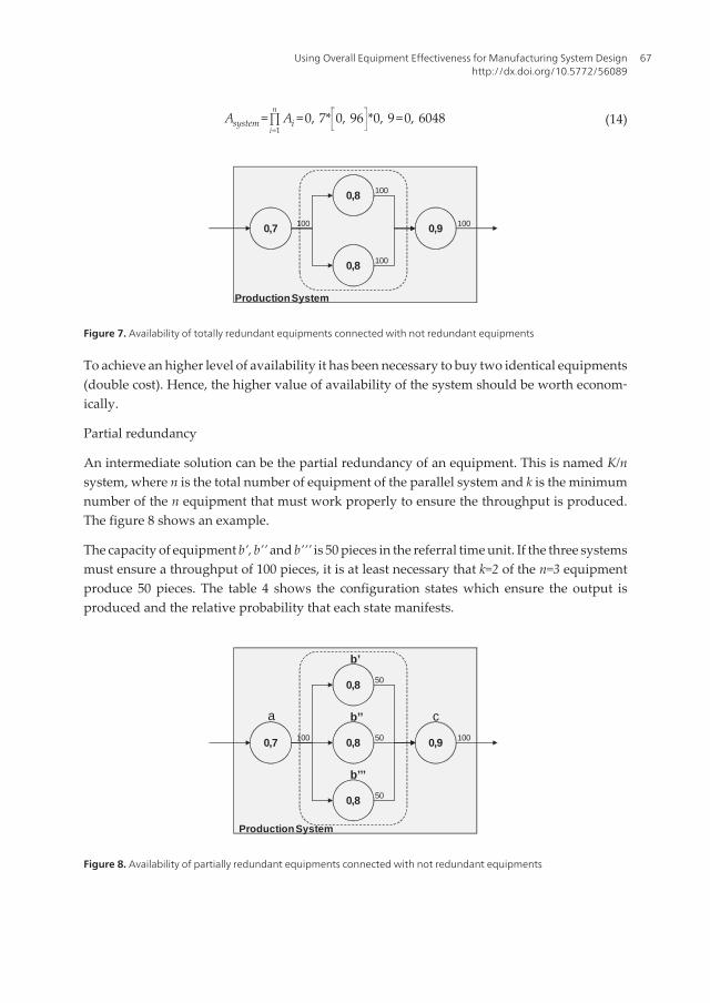
Figure 7. Availability of totally redundant equipments connected with not redundant equipments

To achieve an higher level of availability it has been necessary to buy two identical equipments(double cost). Hence, the higher value of availability of the system should be worth econom‐ically.

Partial redundancy

An intermediate solution can be the partial redundancy of an equipment. This is named K/nsystem, where n is the total number of equipment of the parallel system and k is the minimumnumber of the n equipment that must work properly to ensure the throughput is produced.The figure 8 shows an example.

The capacity of equipment b’, b’’ and b’’’ is 50 pieces in the referral time unit. If the three systemsmust ensure a throughput of 100 pieces, it is at least necessary that k=2 of the n=3 equipmentproduce 50 pieces. The table 4 shows the configuration states which ensure the output isproduced and the relative probability that each state manifests.

0,7

0,8

0,9

Production System

0,8

100

50

50

1000,8 50

a c

b’

b’’

b’’’

Figure 8. Availability of partially redundant equipments connected with not redundant equipments


67

b’ b’’ b’’’ Probability of

occurrance

[*100]

UP UP UP 0,8*0,8*0,8 0,512

UP UP DOWN 0,8*0,8*(1-0,8) 0,128

UP DOWN UP 0,8*(1-0,8)*0,8 0,128

DOWN UP UP (1-0,8)*0,8*0,8 0,128

Total Availability 0,896

Table 4. State Analysis Configuration

In this example all equipments b have the same reliability (0,8), hence the probability the systemof three equipment ensure the output should have been calculated, without the state analysisconfiguration (table 4), through the binomial distribution:

Rk /n = ∑j=k

n (nj )R j 1 - R n- j (15)

R2/3 =(32)0, 82 1 - 0, 8 + (33)0, 83=0,896 (16)

Hence, the availability of the system (a, b’-b’’-b’’’, c) will be:

Asystem =∏i=1

nAi =0, 7* 0, 896 *0, 9=0, 56448 (17)

In this case the investment in redundancy is lower than the previous. It is clear how the choiceof the level of availability is a trade-off between fix-cost (due to equipment investment) andlack of availability.

In all the cases we considered the buffer as null.

When reliability of the equipments (b in our example) the binomial distribution (16) is notapplicable, therefore the state analysis configuration (table 4) is required.

Redundancy with modular capacity

Another configuration is possible.

The production system can be designed as composed of two equipment which singularcapacity is lower than the requested but which sum is higher. In this case if it is possible tomodulate the production capacity of previous and successive stations the expected throughputwill be higher than the output of a singular equipment.


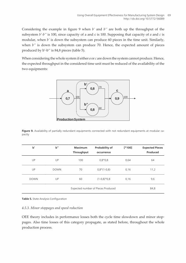
Considering the example in figure 9 when b’ and b’’ are both up the throughput of thesubsystem b’-b’’ is 100, since capacity of a and c is 100. Supposing that capacity of a and c ismodular, when b’ is down the subsystem can produce 60 pieces in the time unit. Similarly,when b’’ is down the subsystem can produce 70. Hence, the expected amount of piecesproduced by b’-b’’ is 84,8 pieces (table 5).

When considering the whole system if either a or c are down the system cannot produce. Hence,the expected throughput in the considered time unit must be reduced of the availability of thetwo equipments:

0,7

0,8

0,9

Production System

0,8

100

70

60

100

b’

b’’

a c

Figure 9. Availability of partially redundant equipments connected with not redundant equipments at modular ca‐pacity

b’ b’’ Maximum

Throughput

Probability of

occurrence

[*100] Expected Pieces

Produced

UP UP 100 0,8*0,8 0,64 64

UP DOWN 70 0,8*(1-0,8) 0,16 11,2

DOWN UP 60 (1-0,8)*0,8 0,16 9,6

Expected number of Pieces Produced 84,8

Table 5. State Analysis Configuration

4.5.3. Minor stoppages and speed reduction

OEE theory includes in performance losses both the cycle time slowdown and minor stop‐pages. Also time losses of this category propagate, as stated before, throughout the wholeproduction process.


69

A first type of performance losses propagation is due to the propagation of minor stoppagesand reduced speed among machines in series system. From theoretical point of view, betweentwo machines with the same cycle time 1and without buffer, minor stoppage and reducedspeed propagate completely like as major stoppage. Obviously just a little buffer can mitigatethe propagation.

Several models to study the role of buffers in avoiding the propagation of performance lossesare available in Buffer Design for Availability literature [22]. The problem is of scientific rele‐vance, since the lack of opportune buffer between the two stations can indeed affect dramat‐ically the availability of the whole system. To briefly introduce this problem we refer to aproduction system composed of two consecutive equipments (or stations) with an interposedbuffer (figure 10).

1 2

Production System

Figure 10. Station-Buffer-Station system. Adapted by [23]

Under the likely hypothesis that the ideal cycle times of the two stations are identical [23], thevariability of speed that affect the stations is not necessarily of the same magnitude, due to itsdependence on several factors. Furthermore Performance index is an average of the T t ,therefore a same machine can sometimes perform at a reduced speed and sometimes an highestspeed2. The presence of this effect in two consecutive equipments can be mutually compensateor add up. Once again, within the propagation analysis for production system design, the roleof buffer is dramatically important.

When buffer size is null the system is in series. Hence, as for availability, speed losses of eachequipment affect the performance of the whole system:

Psystem =∏i=1

nPi (18)

Therefore, for the two stations system we can posit:

1 As shown in par. 3.1. When two consecutive stations present different cycle times, the faster station works with thesame cycle time of slower station, with consequence on equipment OEE, even if any time losses is occurred. On the otherhand, when two consecutive stations are balanced (same cycle time) if any time loss is occurring the two stations OEEwill be 100%. Ideally, the higher value of performance rate can be reached when the two stations are balanced.2 This time losses are typically caused by yield reduction (the actual process yield is lower than the design yield). Thiseffect is more likely to be considered in production process where the equipment saturation level affect its yield, likefurnaces, chemical reactor, etc.


Psystem =∏i=1

2Pi (19)

But when the buffer is properly designed, it doesn’t allow the minor stoppages and speedlosses to propagate from a station to another. We define this Buffer size as Bmax. When, in aproduction system of n stations, given any couple of consecutive station, the interposed buffersize is Bmax (calculated on the two specific couple of stations), then we have:

Psystem =Min i=1n (Pi) (20)

That for the considered 2 stations system is:

Psystem =Min (P1, P2) (21)

Hence, the extent of the propagation of performance losses depends on the buffer size (j) thatis interposed between the two stations. Generally, a bigger buffer increases the performanceof the system, since it increases the decoupling degree between two consecutive stations, upto j=Bmax is achieved (j =0,..,Bmax).

We can therefore introduce the parameter

Rel.P(j)= P ( j)P (Bmax) (22)

Considering the model with two station, figure 11, we have that:

When j = 0, Rel.P (0)= P (0)P(Bmax) = P(1)*P(2) / min(P(1);P(2)); (23)

When j = Bmax, Rel.P (B max)= P (Bmax)P(Bmax) = 1; (24)

Figure 11 shows the trend of Rel.P(j) depending on the buffer size (j), when the performancerate of each station is modeled with an exponential distribution [23] in a flow shop environ‐ment. The two curves represent the minimum and the maximum simulation results. All theothers simulation results are included between these two curves. Maximum curve representsthe configuration with the lowest difference in performance index between the two stations,the minimum the configuration with the highest difference.

By analyzing the figure 11 it is clear how an inopportune buffer size affect the performance ofthe line and how increase in buffer size allows to obtain improve in production line OEE. Bythe way, once achieved an opportune buffer size no improvement derives from a furtherincrease in buffer. These considerations of Performance index trend are fundamental for aneffective design of a production system.


71

50.00%

60.00%

70.00%

80.00%

90.00%

100.00%

110.00%

1 21 41 61 81 101 121 141

Rel

.P(j)

Buffer Size (j)

MIN MAX

Figure 11. Rel OEE depending on buffer size in system affected by variability due to speed losses

4.5.4. Quality losses

In this paragraph we analyze how quality losses propagate in the system and if it is possibleto assess the effect of quality control on OEE and OTE.

First of all we have to consider that quality rate for a station is usually calculated consideringonly the time spent for the manufacturing of products that have been rejected in the samestation. This traditional approach focuses on stations that cause defects but doesn’t allow topoint out completely the effect of the machine defectiveness on the system. In order to do so,the total time wasted by a station due to quality losses should include even the time spent formanufacturing of good products that will be rejected for defectiveness caused by other stations.In this sense quality losses depends on where scraps are identified and rejected. For example,scraps in the last station should be considered loss of time for the upstream station to estimatethe real impact of the loss on the system and to estimate the theoretical production capacityneeded in the upstream station. In conclusion the authors propose to calculate quality rate fora station considering as quality loss all time spent to manufacture products that will notcomplete the whole process successfully.

From a theoretical point of view we could consider the following case for calculation of qualityrate of a station that depends on types of rejection (scraps or rework) and on quality controlspositioning. If we consider two stations with an assigned defectiveness Sj and each stationreworks its scraps with a rework cycle time equal to theoretical cycle time, quality rate couldbe formulate as shown in case 1 in figure 12. Each station will have quality losses (time spentto rework products) due its own defectiveness. If we consider two stations with an assigneddefectiveness Sj and a quality control station at downstream each station, quality rate couldbe formulate as shown in case 2 in figure 12. The station 1, that is the upstream station, will


have quality losses (time spent to work products that will be discarded) due to its own andstation 2 defectiveness. If we consider two stations with an assigned defectiveness Sj andquality control station is only at the end of the line, quality rate quality rate could be formulateas shown in case 3 in figure 12. In this case both stations will have quality losses due to thepropagation of defectiveness in the line. Case 2 and 3 point out that quality losses could be notsimple to evaluate if we consider a long process both in design and management of system. Inparticular in the quality rate of station 1 we consider time lost for reject in the station 2.

C1 2

))(( 2121 11 ssQQ ==

scraps

Case 3)

1 2

)()( 2211 11 sQsQ ==

rework

Case 1)

1 2

)())(( 22211 111 sQssQ ==

scraps

Case 2)

Figure 12. Different cases of quality rate calculation

Finally, it is important to highlight the different role that the quality efficiency plays duringthe design phase and the production.

When the system is producing, Operations Manager focuses his attention on the causes of thedelectability with the aim to reduce it. When it is to design the production system, OperationsManager focuses on the expected quality efficiency of each station, on the location of qualitycontrol, on the process (rework or scraps) to identify the correct number of equipments orstation for each activity of the process.

In this sense, the analysis is vertical during the production phase, but it follows the wholeprocess during the design (figure 13).

1 2 i n-1 n

Production

Figure 13. Two approaches for quality efficiency

5. The simulation model

To study losses propagation and to show how these dynamics affect OEE in a complex system[25] this chapter presents some examples taken from an OEE study of a real manufacturingsystem carried out by the authors through a process simulation analysis [19].


73

Simulation is run for each kind of time losses (Availability, Performance and Quality), toclearly show how each equipment ineffectiveness may compromise the performance of thewhole system.

The simulation model is about a manufacturing plant for production of electrical cable. Inparticular we focuses on production of unipolar electrical cable that takes place by a flow-shopprocess. In the floor plant the production equipment is grouped in production areas arrangedaccording to their functions (process layout). The different production areas are located alongthe line of product flow (product layout). Buffers are present amongst the production areas tostock the product in process. This particular plant allows to analyze deeply the problem ofOEE-OTE investigation due to its complexity.

In terms of layout the production system was realized as a job shop system, although the flowof material from a station to another was continuous and typical of flow shop process. As statedin (§2) the reason lies on due to the huge size of the products that passes from a station toanother. For this reason the buffer amid station, although present, couldn’t contain hugeamount of material.

The process implemented in the simulation model is shown in figure 14. Entities are unitquantity of cable that have different mass amongst stations. Parameters that are data input inthe model are equipment speed, defectiveness, equipment failure rate and mean time to repair.Each parameters is described by a statistical distribution in order to simulate random condi‐tion. In particular equipment speed has been simulated with a triangular distribution in orderto simulate performance losses due to speed reduction.

The model evaluates OTE and OEE for each station as usually measured in manufacturingplant. The model has been validated through a plan of tests and its results of OEE has beencompared with results obtained from an analytic evaluation.

Roughing Drawing Bunching Insulating Packaging

Figure 14. ASME representation of manufacturing process

5.1. Example of availability losses propagation

In accordance with the proposed method (§ 3.5) we show how availability losses propagate inthe system and to assess the effect of buffer capacity on OEE through the simulation. Wefocuses on the insulating and packaging working stations. Technical data about availability ofequipment are: mean time between failure for insulating is 20000 sec while for packaging is30000 sec; mean time between repair for insulating is 10000 sec while for packaging is 30000sec. The cycle time of the working stations are the same equal to 2800 sec for coil. The qualityrates are set to 1. Idling, minor stoppages and reduced speed are not considered and set to 0.


Considering equipment isolated from the system the OEE for the single machine is equal toits availability; in particular, relating to previous data, machines have an OEE equal to 0,67and 0,5 respectively for insulating and packaging. The case points out how the losses due tomajor stoppage spread to other station in function of buffer capacity dimension.

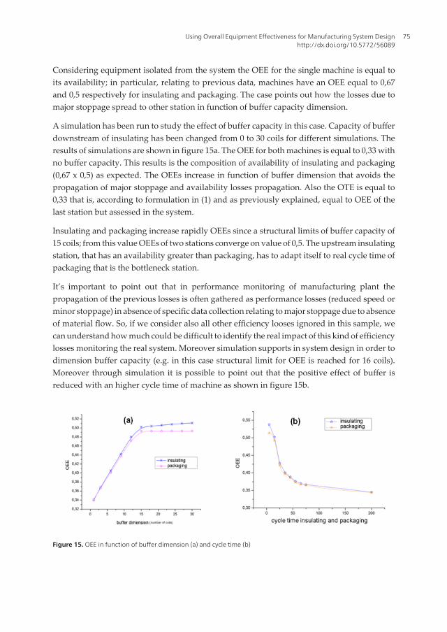
A simulation has been run to study the effect of buffer capacity in this case. Capacity of bufferdownstream of insulating has been changed from 0 to 30 coils for different simulations. Theresults of simulations are shown in figure 15a. The OEE for both machines is equal to 0,33 withno buffer capacity. This results is the composition of availability of insulating and packaging(0,67 x 0,5) as expected. The OEEs increase in function of buffer dimension that avoids thepropagation of major stoppage and availability losses propagation. Also the OTE is equal to0,33 that is, according to formulation in (1) and as previously explained, equal to OEE of thelast station but assessed in the system.

Insulating and packaging increase rapidly OEEs since a structural limits of buffer capacity of15 coils; from this value OEEs of two stations converge on value of 0,5. The upstream insulatingstation, that has an availability greater than packaging, has to adapt itself to real cycle time ofpackaging that is the bottleneck station.

It’s important to point out that in performance monitoring of manufacturing plant thepropagation of the previous losses is often gathered as performance losses (reduced speed orminor stoppage) in absence of specific data collection relating to major stoppage due to absenceof material flow. So, if we consider also all other efficiency looses ignored in this sample, wecan understand how much could be difficult to identify the real impact of this kind of efficiencylosses monitoring the real system. Moreover simulation supports in system design in order todimension buffer capacity (e.g. in this case structural limit for OEE is reached for 16 coils).Moreover through simulation it is possible to point out that the positive effect of buffer isreduced with an higher cycle time of machine as shown in figure 15b.

Figure 15. OEE in function of buffer dimension (a) and cycle time (b)


75

5.2. Minor stoppages and speed reduction

We run the simulation also for the case study (§ 4). The simulation shown how two stations,with the same theoretical cycle time (200 sec/coil) affected by a triangular distribution with aperformance rate of 52% as single machine, have: 48% of performance rate with a capacitybuffer of 1 coil and 50% of performance rate with a capacity buffer of 2 coils. But if we considertwo stations with the same theoretic cycle time but affects by different triangular distributionsso that theoretic performance rates differ, simulation shows how the performance rates of twostations converge towards the lowest one as expected (19), (20).

Through the same simulation model we considered also the second type of performancelosses propagation, due to the propagation of reduced speed caused by unbalanced line.Figure 16 shown the effect of unbalanced cycle time of stations relating to insulating andpackaging. The station have the same P as single machine equal to 67% but differenttheoretical cycle time. In particular insulating, the upstream station, is faster than packag‐ing. Availability and quality rate of stations is set to 1. The buffer capacity is set to 1 coil.A simulation has been run to study the effect of unbalancing station. Theoretical cycle timeof insulating has been changed since theoretical cycle time of packaging that is fixed inmean. The simulation points out that insulating has to adapt itself to cycle time of packagingthat is the bottleneck station. This results in the model as a lower value for performancerate of insulating station. The same happens often in real systems where the result isinfluenced by all the efficiency losses at the same time. The effect disappears gradually witha better balancing of two stations as in figure 16.

per

form

ance

rat

e

Figure 16. Performance rate of insulating and packaging in function of insulating cycle time

5.3. Quality losses

In relation to the model, this sample focuses on the drawing and bunching working stationsthat have defectiveness set to 5%, the same cycle times and no other efficiency losses. Thequality control has been changed simulating case 2 and 3. The results of simulation for the two


cases are shown in table 6 in which the proposal method has compared with the traditionalone. The proposal method allowed to identify the correct efficiency, for example to dimensionthe drawing station, because it considers time wasted to manufacture products rejected inbunching station. The difference between values of Q2 and OTE is explained by the value ofP2=0,95 that is due to the propagation of quality losses for the upstream station in performancelosses for the downstream station. Moreover about positioning of quality control the case 2has to be prefer because the simulation shows a positive effect on the OTE if the bunchingstation is the system bottleneck (as it happens in the real system).

Proposal method Traditional method

Q1 Q2 OTE Q1 Q2 OTE

Case 2) 0,952 0,95 0,952 0,95 0,95 0,952

Case 3) 0,952 0,952 0,952 -- 0,952 0,952

Table 6. Comparison of quality rate calculation and evaluation of impact of quality control positioning on quality ratesand on OTE

6. Conclusions

The evaluation of Overall Equipment Effectiveness (OEE) and Overall Throughput Effective‐ness (OTE) can be critical for the correct estimation of workstations number needed to realizethe desired throughput (production system design), as also for the analysis and the continuousimprovement of the system performance (during the system management).

The use of OEE as performance improvement tool has been widely described in the literature.But it has been less approached in system design for a correct evaluation of the systemefficiency (OTE), in order to study losses propagation, overlapping of efficiency losses andeffective actions for losses reduction.

In this chapter, starting by the available literature on time losses, we identified a simplified setof relevant time-losses that need to be considered during the design phase. Then, through thesimulation, we shown how OEE of single machine and the value of OTE of the whole systemare interconnected and mutually influencing each other, due to the propagation of availability,performance and quality losses throughout the system.

For each category of time losses we described the effects of efficiency losses propagation froma station to the system, for a correct estimation and analysis of OEE and OTE during manu‐facturing system design. We also shown how to avoid losses propagation through adequatetechnical solutions which can be defined during system design as the buffer sizing, theequipment configuration and the positioning of control stations.

The simulation model shown in this chapter was based on a real production system and it usedreal data to study the losses propagation in a manufacturing plant for production of electrical


77

cable. The validation of the model ensures the meaningful of the approach and of the identifiedset of possible solutions and hints.

By analyzing and each time losses we also shown how the choices taken during the design ofthe production system to increase the OTE (e.g. buffer size, maintenance configuration, etc.)affect the successive management of the operations.

Acknowledgements

The realization of this chapter would not have been possible without the support of a personwhose cooperated with the chair of Operations Management of University of Rome “TorVergata” in the last years, producing valuable research. The authors wish to express theirgratitude to Dr. Bruna Di Silvio without whose knowledge, diligence and assistance this workwould not have been successful.

Author details

Vittorio Cesarotti1, Alessio Giuiusa1,2 and Vito Introna1

1 University of Rome “Tor Vergata”, Italy

2 Area Manager Inbound Operations at Amazon.com

References

[1] H. H. S., «Manufacturing productivity improvement using effectivenes metrics andsimulation analysis,» 2002.

[2] B. I., «Effective measurement and successful elements of company productivity: thebasis of competitiveness and world prosperity,» International Journal of ProductionEconomics, vol. 52, pp. 203-213, 1997.

[3] Jeong, P. D. K.Y., «Operational efficiency and effectiveness measurement,» Interna‐tional Journal of Operations and Production Management, n. 1404-1416, (2001). , 21

[4] N. S., Introduction to TPM- Total Productive Maintenance, Productivity Press, 1988.

[5] S. R.J., World Class Manufacturing. The lesson of simplicity Applied, The Free Press,1987.

[6] Womack, J. D. J.P., Lean Thinking, Simon & Schuster, (1996).


[7] Dixon, N. A. V. J.R., The new performance challenge. Measuring operations forworld-class competition, Dow Jones Irwin, (1990).

[8] S. D., «Can CIM improve overall factory effetivenes,» in Pan Pacific MicroelectronicSymposium, Kauai, HI, 1999.

[9] Waters, W. D. D.J., Operations Management, Kogan Page Publishers, (1999).

[10] Chase, A. N. J. F. R.B., Operations Management, McGraw-Hill, (2008).

[11] A. V. A., Semiconductor Manufacturing Productivity- Overall Equipment Effective‐ness (OEE) guidebook, SEMATECH, 1995.

[12] Rooda, D. R. A. J. J.E., «Equipment effectiveness: OEE revisited,» IEEE Transactions onSemiconductor Manufacturing, n. 1, (2005). , 18 , 189-196.

[13] Gamberini, G. L. R. B. R., «Alternative approaches for OEE evaluation: some guide‐lines directing the choice,» in XVII Summer School Francesco Turco, Venice, (2012).

[14] Grando, T. F. A., «Modelling Plant Capacity and Productivity,» Production Planningand Control, n. 3, (2005). , 16 , 209-322.

[15] Spada, C. V. C., «The Impact of Cultural Issues and Interpersonal Behavior on Sus‐tainable Excellence and Competitiveness: An Analysis of the Italian Context,» Contri‐butions to Management Science, (2008). , 95 - 113 .

[16] Badiger, G. R, & Proposal, A. , «A. evaluation of OEE and impact of six big losses onequipment earning capacity,» International Journal Process Management & Benchmark‐ing, (2008). , 235 - 247 .

[17] Jacobs, A. N. C. B, & Operations, R. F. and supply chain management, McGraw-Hill,A cura di, (2010).

[18] Oechsner, R. From overall equipment efficiency(OEE) to overall Fab effectiveness(OFE),» Materials Science in Semiconductor Processing, (2003). , 5 , 333-339.

[19] Introna, D. S. B. C. V, & Flow-shop, V. process oee calculation and improvement us‐ing simulation analysis,» in MITIP, Florence, (2007).

[20] R. MA, «Factory Level Metrics: Basis for Productivity Improvement,» in Proceedingsof the International Conference on Modeling and Analysis of Semiconductor, Tempe, Arizo‐na, USA, 2002.

[21] Scott, P. R. D., «Can overall factory effetiveness prolong Moore’s Law?,» Solid StateTechnology, (1998). , 41 , 75-82.

[22] B. D., «Buffer size design linked to reliability performance: A simulative study,»Computers & Industrial Engineering, vol. 56, p. 1633-1641, 2009.

[23] Introna, G. A. V. V., «Increasing Availability of Production Flow lines through Opti‐mal Buffer Sizing: a Simulative Study,» in The 23rd European Modeling & SimulationSymposium (Simulation in Industry), Rome, (2011).


79

[24] Connor, P. D. T. O. Practical Reliability Engineering (Fourth Ed.), New York: JohnWiley & Sons, (2002).

[25] Kane, J. O. Simulating production performance: cross case analysis and policy impli‐cations,» Industrial Management & Data Systems, n. 4, (2004). , 104 , 309-321.

[26] Gondhinathan, B. A, & Proposal, R. , «A. evaluation of OEE and impact of six biglosses on equipment earning capacity,» International Journal Process Management &Benchmarking, n. 3, (2008). , 2 , 235-247.


Date post:	02-Mar-2019
Category:	Documents
Upload:	vandang
View:	216 times
Download:	0 times

Using Overall Equipment Effectiveness for Manufacturing...

Documents