Dartmouth College | Research Computing

USING R FOR BASIC SPATIAL ANALYSIS

• Research Computing and Spatial Analysis at Dartmouth

• What is Spatial Analysis?

• What is R?

• Basics of R

• Common Spatial Packages for R

• Viewing and analyzing Spatial Data in R

• Hands-on practice

• Display in GIS software

• Questions and Wrap-up

OVERVIEW

RESEARCH COMPUTING AT DARTMOUTH

• Research Computing• Workshops

• Storage

• Consulting

• Software

• Hardware

• Visit our website, http://rc.dartmouth.edu/

• Request a research account

• Email us• research.computuing@da

rtmouth.edu

• stephen.p.gaughan@dartmouth.edu

Mission: Promote the advancement of research through the use of high-performance computing (HPC), life sciences support and bioinformatics, GIS consulting, services and workshops

• Courses in the Geography Department and the Earth Sciences Department, GIS and spatial analysis

• Geography Department http://geography.dartmouth.edu/

• Geog 50 Geographic Information Systems

• Geog 57 Urban Applications of GIS

• Geog 51 / Ears 65: Remote Sensing

• Geog 54 Geovisualization

• Geog 59/Ears 77 Environmental Applications of GIS

• Dartmouth College Library: Library Reference Research Guides for the R statistical package, GIS and spatial analysis

• GIS http://researchguides.dartmouth.edu/gis

• Statistics, R http://researchguides.dartmouth.edu/statapp_koujue

• Research Computing

SPATIAL ANALYSIS AT DARTMOUTH

• Data Visualization using R

• James Adams, Baker-Berry Library, James.L.Adams@dartmouth.edu

• Statistical Consulting (R, Stata, SAS)

• Jianjun Hua from Ed Tech provides consulting support for statistics-related questions. Jianjun can be contacted at 603-646-6552 or by emailing jianjun.hua@dartmouth.edu

• R for High Performance Computing, parallel computing, GIS

• Research.computing@Dartmouth.edu and http://rc.dartmouth.edu/

• R Club

• Katja Koeppen, Microbiology Department organizes an R Club, Katja.Koeppen@Dartmouth.edu

• Programming n’ Pizza http://rc.dartmouth.edu/index.php/programming-n-pizza/

• Departmental Courses at Dartmouth, Statistics, Math, Quantitative Social Sciences, etc

• Math 10, Math 50 https://math.dartmouth.edu/courses/by-term/ , http://qss.dartmouth.edu/

• Math 10, Online Stats book “Online Statistics Education: A Multimedia Course of Study” (http://onlinestatbook.com/ ). David M. Lane, Rice University.

MORE INFO

• Spatial analysis is the application of analysis tools to spatial data

• Spatial data includes geographic data in both raster and vector formats, for example:

• Vector data – points, lines and regions (polygons)

• Raster data – gridded data such as satellite imagery, elevation data across a surface, rainfall totals across a surface over a given period of time

WHAT IS SPATIAL ANALYSIS?

• R is a free software environment used for computing, graphics and statistics. It comes with a robust programming environment that includes tools for data analysis, data visualization, statistics, high-performance computing and geographic analysis. Visit https://www.r-project.org/ for more

• R has been around for more than 20 years and it has become popular at universities, research labs and federal and state government offices in the last ten years for many applications

• R consists of base packages but also includes hundreds of add-on packages that greatly extend the capabilities of the programming environment.

• These capabilities include data manipulation, data visualization and spatial analysis tools

• CRAN-Spatial is located here: https://cran.r-project.org/web/views/Spatial.html

• If you are already a GIS user, you’ll notice similar commands and techniques, and of course, you’ll recognize spatial data when displayed on a map in R

WHAT IS R?

• The R console is a quick, light, multiplatform install

BASICS OF R (I)THE R CONSOLE

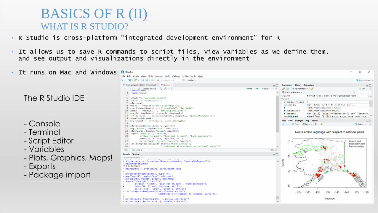
• R Studio is cross-platform “integrated development environment” for R

• It allows us to save R commands to script files, view variables as we define them, and see output and visualizations directly in the environment

• It runs on Mac and Windows

BASICS OF R (II)WHAT IS R STUDIO?

The R Studio IDE

- Console- Terminal- Script Editor- Variables- Plots, Graphics, Maps!- Exports- Package import

• https://support.rstudio.com/hc/en-us/articles/201057987-Quick-list-of-useful-R-packages

• Tidyr

• Ggplot2

• Dpylr

• xlsx

• Maps

• Sp

• Rgdal

• Parallel

BASICS OF R (III)SOME PACKAGES TO EXTEND R

• Spatial:

• SP “spatial”

• GSTAT “geostatistics”

• RGDAL “geospatial data abstraction library for R”

• MAPS “maps”

• GGMAP “extends the plotting of ggplot2 with map data”

• RASTER “raster data processing”

• MAPTOOLS “map tools”

• SPATSTAT “wide range of spatial tools and functions”

COMMON SPATIAL PACKAGES FOR R

VIEWING AND ANALYZING SPATIAL DATA (I)

• Put a Google base map right in your plot window, overlay spatial data on to the map plot

12

Map overlay & spatial statistics

Packages sp, rgdal and maps can turn your R in to a GIS: read, write and analyze spatial data, map overlay

VIEWING AND ANALYZING SPATIAL DATA (I)GEOGRAPHIC INFORMATION ANALYSIS

• ?setwd

• Help(setwd)

• Web Searches

• Google ‘r set working directory’

• Stack Overflow ‘r set working directory stack overflow’

HELP IN R

READY TO DIVE IN?

• We’ll use R Studio today so we can see our spatial analysis and work with R script files

• Open R Studio

• In the “Console” at the “greater than” symbol, enter:

> install.pakages(“maps”)

• Continue on in R Studio, entering the following commands:

GETTING STARTED

install.packages("ggmap")library(maps)library(ggmap)

visited <- c("Boston, MA", "Anchorage, AK")ll.visited <- geocode(visited)visit.x <- ll.visited$lonvisit.y <-ll.visited$lat

GETTING STARTED

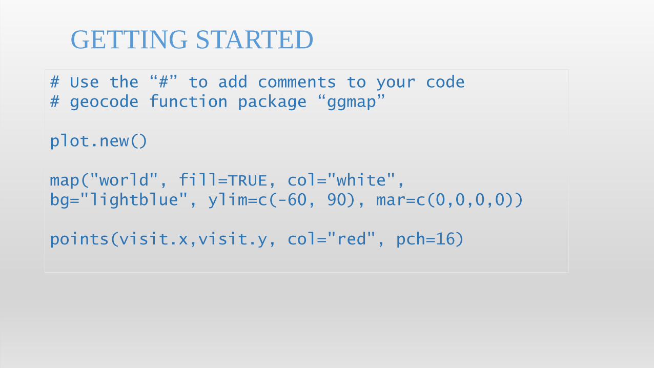
# Use the “#” to add comments to your code # geocode function package “ggmap”

plot.new()

map("world", fill=TRUE, col="white", bg="lightblue", ylim=c(-60, 90), mar=c(0,0,0,0))

points(visit.x,visit.y, col="red", pch=16)

• The “geocoded” data should now show up in R Studio’s plots window, shown on a map of the world

VIEW THE RESULTS

• Enter the following in to the R Studio command line

MAP A COORDINATE PAIR

install.packages("ggplot2")

library(ggplot2)library(ggmap)

# This line is a comment plot in window

mapHanover <- get_map("Hanover, NH", zoom=10)

ggmap(mapHanover)

mapLatLong <- get_map(location = c(lon = -71.0712, lat = 42.3538))

ggmap(mapLatLong)

• To make R code easier to type in, save and re-use, we can use an R Script file.

• In R Studio, click File > New File > R Script

USING R SCRIPT FILES

• Here we see the code inside a “.R” file

• Code can be run line-by-line using the “Run” button in the upper bar

USING R SCRIPT FILES

• Open R Studio (All Programs > R Studio)

• Downloading the Data:• In your browser, type dartgo.org/rspatial

• At the DartBox site, click the ellipses ... and choose ‘Download’

• Download file Student.zip

• Copy the file to a convenient location such as:

c:\rworkspace

• Unzip the file

WORKING WITH SPATIAL DATA

READY TO DIVE IN?

• We’ll use R Studio today so we can see our spatial analysis

• Data for this session can be downloaded at:

dartgo.org/rspatial

• Download file and unzip

• Copy the file to a “Working Directory” that R will recognize

• Use the “getwd()” and “setwd()” commands in R, and your computer’s file browser (Finder on the Mac, Windows Explorer on the PC)

GETTING THE DATA AND R TO WORK TOGETHER

On the PC:

getwd()

[1] "C:/Users/f002d69/Documents"

> setwd("c:/users")

> getwd()

[1] "c:/users"

>

On the mac:

getwd()

[1] "/Users"

> setwd("~/Desktop")

> getwd()

[1] "/Users/sgaughan/Desktop"

MAP OVERLAY, POINT-IN-POLYGON ANALYSIS WITH SP “OVER” FUNCTION

• Packages “sp”, “rgdal” and “maps” can turn your R into a GIS

• Read-Write and Analyze spatial data, perform “map overlay”

install.packages(“sp”)install.packages(”rgdal”)install.packages(”maps”)library(sp)library(rgdal)library(maps)

# load a csv with latitude and longitude coordinates

bears <- read.csv("bear-sightings.csv")

coordinates(bears) <- c("longitude", "latitude")

# load a shapefile representing an area

parks <- readOGR(".", "10m_us_parks_area")

25

MAP OVERLAY, POINT-IN-POLYGON ANALYSIS WITH SP “OVER” FUNCTION

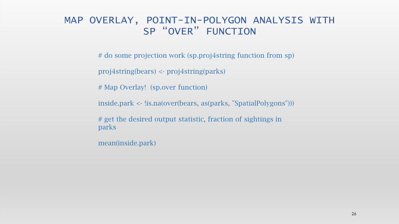
# do some projection work (sp.proj4string function from sp)

proj4string(bears) <- proj4string(parks)

# Map Overlay! (sp.over function)

inside.park <- !is.na(over(bears, as(parks, "SpatialPolygons")))

# get the desired output statistic, fraction of sightings in parks

mean(inside.park)

26

PLOT THE POINTS AND EXPORT

bears$park <- over(bears, parks)$Unit_Name

# Put the data on the map in just a few lines!

plot(coordinates(bears), type="n")

# use the maps.map function

map("world", region="usa", add=TRUE)

# …and the sp.plot function

plot(parks, border="green", add=TRUE)

points(bears[!inside.park, ], pch=1, col="gray")

27

PLOT THE POINTS AND EXPORT

points(bears[inside.park, ], pch=16, col="red")

# Export GIS data or flat-file data

write.csv(bears, "bears-by-park.csv", row.names=FALSE)

# Export a GIS format ‘shapefile’ using the rgdal.writeOGR funtion

writeOGR(bears, ".", "bears-by-park", driver="ESRI Shapefile")

28

ADDING A LEGEND AND TITLE# add a legend

legend("topright", cex=0.85,c("Bear in park", "Bear not in park", "Park boundary"),pch=c(16, 1, NA), lty=c(NA, NA, 1),col=c("red", "grey", "green"), bty="n")

# add a title

title(expression(paste(italic("Ursus arctos")," sightings with respect to national

parks")))

29

# The “#” is a “comment”. No need to type these lines # note: package "sp" might ask to restart your R session

install.packages("sp")install.packages("rgdal")

# import libraries

library(gstat)library(sp)library(rgdal)

INSTALL SPATIAL LIBRARIES “GSTAT”, “SP” AND “GDAL”

# load the meuse dataset in to the Rstudio environment

data(meuse)

# retrieve/set spatial coord

coordinates(meuse) = ~x+y

# note: coordinates use projection # EPSG:28992 Amersfoort/RD Netherlands DutchRD# view the first 5 coordinate pairs

coordinates(meuse)[1:5,]

# plot the zinc concentrations (bubble plot,# high levels with larger circles)

bubble(meuse, "zinc", col=c("#00ff0088", "#00ff0088"), main = "zinc concentrations (ppm)")

LOAD DATASET IN TO R STUDIO AND PLOT

examine the "meuse" dataset, point data set consists of 155 samples of top soil heavy metal concentrations (ppm), along with a number of soil and landscape variables. The samples were collected in a flood plain of the river Meuse, near the village Stein, southern Netherlands, 50.9686432 Lat,5.7460789 Longitude

# Task 2: distance display# load the meuse.grid datadata(meuse.grid)class(meuse.grid) # dataframesummary(meuse.grid)

coordinates(meuse.grid) = ~x+y # convert to spatialpontsdataframeclass(meuse.grid)

# set the gridded function to "TRUE", which converts class to SpatialPixelsDataFramegridded(meuse.grid) = TRUE class(meuse.grid)# clear the plot window dev.off()# plot image of grid using the distance fieldimage(meuse.grid["dist"])

# add a title to the plottitle("Distance to River meuse.grid(dist), red = 0")

DISPLAY THE DISTANCE TO RIVER

USE THE “GSTAT” PACKAGE FOR THE “INVERSE DISTANCE WEIGHTED” TOOL

# use the gstat "Inverse distance weighted" tool

library(gstat)zinc.idw <- idw(zinc~1, meuse, meuse.grid)

class(zinc.idw)

# spatialPixelsDataFrame

spplot(zinc.idw["var1.pred"], main = "zinc inverse distance weighted interpolations")

Inverse Distance Weighting (IDW) is a GIS function that uses a deterministic method for multivariate interpolation with a known scattered set of points. Unknown points are calculated with a weighted average of the values available at the known points. This function can be used to create surfaces and index layers based on discrete observations. Temperature, elevation are examples.

Reference: https://docs.qgis.org/2.2/en/docs/gentle_gis_introduction/spatial_analysis_interpolation.html

EXAMINE LINEARITY

# in the previous plot, it # appears #that measurements #of high concentrations# of zinc are, in general, #closer to the river# lets linearize this:

plot(log(zinc)~sqrt(dist), meuse)abline(lm(log(zinc)~sqrt(dist), meuse))

LOAD THE LINEAR MODEL AND SUMMARIZE

#load the linear model in to an objectzinc.lm <- lm(log(zinc) ~ sqrt(dist), data=meuse)# show summary of the linear modelsummary(zinc.lm)

Residuals:Min 1Q Median 3Q Max

-1.04624 -0.29060 -0.01869 0.26445 1.59685

Coefficients:Estimate Std. Error t value Pr(>|t|)

(Intercept) 6.99438 0.07593 92.12 <2e-16 ***sqrt(dist) -2.54920 0.15498 -16.45 <2e-16 ***---Signif. codes: 0 ‘***’ 0.001 ‘**’ 0.01 ‘*’ 0.05 ‘.’ 0.1 ‘ ’ 1

Residual standard error: 0.4353 on 153 degrees of freedomMultiple R-squared: 0.6388, Adjusted R-squared: 0.6364 F-statistic: 270.6 on 1 and 153 DF, p-value: < 2.2e-16

KRIGING WITH GSTAT

lznr.vgm = variogram(log(zinc)~sqrt(dist), meuse)lznr.fit = fit.variogram(lznr.vgm, model = vgm(1, "Exp", 300, 1))

lzn.kriged = krige(log(zinc)~1, meuse, meuse.grid, model = lznr.fit)

# the values are INTERPOLATED/ PREDICTED by the original dataset and the kriging function

spplot(lzn.kriged["var1.pred"])

Kriging is a multistep GIS surface creation tool. It explores statistical analysis of the point values and their distances and then creates the surface of interpolated values. Kriging often used when there is a spatially correlated distance or directional bias in the data. It is often used in soil science and geology.

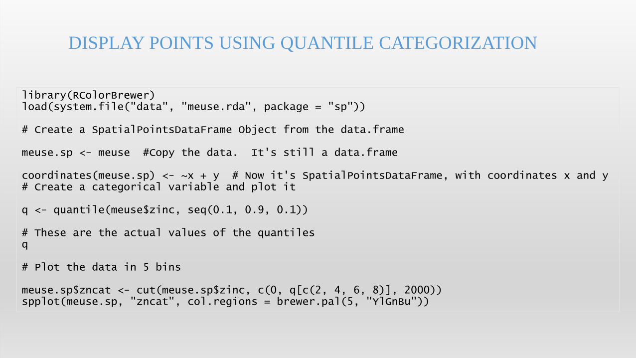
DISPLAY POINTS USING QUANTILE CATEGORIZATION

library(RColorBrewer)load(system.file("data", "meuse.rda", package = "sp"))

# Create a SpatialPointsDataFrame Object from the data.frame

meuse.sp <- meuse #Copy the data. It's still a data.frame

coordinates(meuse.sp) <- ~x + y # Now it's SpatialPointsDataFrame, with coordinates x and y# Create a categorical variable and plot it

q <- quantile(meuse$zinc, seq(0.1, 0.9, 0.1))

# These are the actual values of the quantilesq

# Plot the data in 5 bins

meuse.sp$zncat <- cut(meuse.sp$zinc, c(0, q[c(2, 4, 6, 8)], 2000))spplot(meuse.sp, "zncat", col.regions = brewer.pal(5, "YlGnBu"))

SEND THE POINTS TO A GOOGLE MAPS HTML PAGE

install.packages("plotGoogleMaps")library(plotGoogleMaps)data(meuse)coordinates(meuse)<-~x+y # convert to SPDF

# use CRS from the sp pacakate to indicate the map projection/coord ref system

proj4string(meuse) <- CRS('+init=epsg:28992')

# Adding Coordinate Referent Sys.# Create web map of Point data

m<-plotGoogleMaps(meuse,filename='myMap1.htm')# Plotting another map with icons as pie chart

m<-segmentGoogleMaps(meuse, zcol=c('zinc','dist.m'),mapTypeId='ROADMAP', filename='myMap4.htm',colPalette=c('#E41A1C','#377EB8'), strokeColor='black')

SHOW “MEUSE” DATA IN GOOGLE MAPS WITH “PLOTGOOGLEMAPS” LIBRARY

DATA IN GIS SOFTWARE

R AND GIS- MORE LINKS AND REFERENCES -

• R-GIS Tutorials• https://cran.r-project.org/doc/contrib/intro-spatial-rl.pdf• https://pakillo.github.io/R-GIS-tutorial/#intro

• Visualization, analysis and resources for R and Spatial Data• http://spatial.ly/r/

• Creating maps in R https://github.com/Robinlovelace/Creating-maps-in-R

• Using “Leaflet” maps in R https://github.com/rstudio/leaflet

• National Center for Ecological Analysis: https://www.nceas.ucsb.edu/scicomp/usecases

• https://www.nceas.ucsb.edu/~frazier/RSpatialGuides/ggmap/ggmapCheatsheet.pdf

• http://www.maths.lancs.ac.uk/~rowlings/Teaching/UseR2012/cheatsheet.html

• http://spatial.ly/wp-content/uploads/2013/12/spatialggplot.zip

41

MORE LINKS AND REFERENCES

• http://www.r-bloggers.com/r-beginners-plotting-locations-on-to-a-world-map/

• http://www.kevjohnson.org/making-maps-in-r/

• GGMAPS ( depends on GGPLOT2, imports RGoogleMaps

• https://cran.r-project.org/web/packages/ggmap/index.html

• Spatial References (map projections & coordinate systems)

• http://spatialreference.org/ref/epsg/

• Online Tutorials

• Lynda Tutorials for GIS, R https://www.lynda.com/

• ESRI Tutorials

• GIS Lounge - http://www.gislounge.com/tutorials-in-gis/

42

OTHER SPATIAL FUNCTIONS AND PACKAGES

• Spatial Buffer - package: rgeos, function name: gBuffer

• Near - package: rgeos, function name: gDistance

• Calculate slope of a surface from elevation dataset -package: raster, function name: terrain

• Raster values to points – package: raster, function name: extract

• Proximity Analysis, Hotspot analysis, density analysis

43

OTHER SPATIAL FUNCTIONS AND PACKAGES# Export to KML with rgdal package, import well-formatted KML fileswriteOGR(locs.gb, dsn = "locsgb.kml", layer = "locs.gb", driver = "KML")newmap <- readOGR("locsgb.kml", layer = "locs.gb")

Make data spatial with sp packagecoordinates(locs) <- c("lon", "lat") # set spatial coordinates plot(locs)

# Define a projectioncrs.geo <- CRS("+proj=longlat +ellps=WGS84 +datum=WGS84") # geographical, datum WGS84 proj4string(locs) <- crs.geo # define projection system of our data summary(locs)

# Plot on a simple mapplot(locs, pch = 20, col = "steelblue") library(rworldmap) # library rworldmap provides different types of global maps, e.g: data(coastsCoarse) data(countriesLow) plot(coastsCoarse, add = T)

44

OTHER SPATIAL FUNCTIONS AND PACKAGES# write to shapefile writePointsShape(locs.gb, "locsgb")

# Read shapefilegb.shape <- readShapePoints("locsgb.shp") plot(gb.shape)

# geostatslibrary(gstat) library(geoR)library(akima) # for spline interpolationlibrary(spdep) # dealing with spatial dependence

45

QUESTIONS?

46

MAP PROJECTIONS

• To represent our three-dimensional earth (an ellipsoid) in two dimensions, datums and map projections are used

Projecting a 3D ellipsoid to a 2D computer screen or piece of paper will distort one or more of the following: - shape- distance- area - direction

Projections are sometimes designed to minimize one of these

47

• Data Frames

• CSV format (clean csv)

• Tidy Data

• Other formats - Reading out of databases (SQL), Geographic data constructs

DATA MANAGEMENT