USING SATELLITE IMAGES TO STUDY TEMPORAL CHANGES IN THE MISSISSIPPI DELTA A THESIS SUBMITTED TO THE GLOBAL ENVIRONMENTAL SCIENCE UNDERGRADUATE DIVISION IN PARTIAL FULFILLMENT OF THE REQUIREMENTS FOR THE DEGREE OF BACHELOR OF SCIENCE IN GLOBAL ENVIRONMENTAL SCIENCE AUGUST 2017 By RACHEL CHANG Thesis Advisor DR. PETER MOUGINIS-MARK
Transcript
USING SATELLITE IMAGES TO STUDY TEMPORAL CHANGES IN THE
MISSISSIPPI DELTA
A THESIS SUBMITTED TO THE GLOBAL ENVIRONMENTAL SCIENCE
UNDERGRADUATE DIVISION IN PARTIAL FULFILLMENT OF THE REQUIREMENTS FOR THE DEGREE OF
BACHELOR OF SCIENCE
IN
GLOBAL ENVIRONMENTAL SCIENCE
AUGUST 2017
By RACHEL CHANG
Thesis Advisor
DR. PETER MOUGINIS-MARK
iv
I certify that I have read this thesis and that, in my opinion, it is satisfactory in scope and quality as a thesis for the degree of Bachelor of Science in Global Environmental Science.
THESIS ADVISOR
________________________________ Peter Mouginis-Mark
Hawaii Institute of Geophysics and Planetology
iv
ACKNOWLEDGEMENTS
First and foremost I would like to acknowledge and thank my advisor Dr. Peter
Mouginis-Mark. Thank you Pete for all of your knowledge, guidance and patience over
the past few years. Thank you to the NASA Hawaii Space Grant Consortium for allowing
me to explore aspects of this project through a traineeship. I would also like to thank the
Global Environmental Science community, Michael Guidry, Kristin Momohara and
Catalpa Kong for all your support throughout my academic career. The journey through
this program would not be possible without you. Lastly, a big mahalo to my family and
friends for the continuous support.
iv
ABSTRACT
Satellite images are able to provide unique perspectives of the planet, which can
be used to observe changes over time. I investigated the Mississippi Delta and observed
changes in shorelines using satellite images and tidal data. Images collected by Landsat
and Google Earth ranging from the 1980s to the present were compared with other
images taken at the same tide to observe change. The images were compared to sediment
data to determine shoreline changes in the area, due to both sea level rise and sinking
land. There is a relationship between sea level rise and shoreline change, which can be
observed by using satellite images. The impact of Hurricane Katrina, a major storm event
in August 2005, was studied. Overall, this one-time event affected most shorelines in the
area, but little long-term impact. This study provides a method to study temporal changes
in the Mississippi Delta, though other low-lying coastal areas can benefit from satellite
data these methods.
v
Table of Contents ACKNOWLEDGEMENTS ................................................................................................ 3
ABSTRACT ....................................................................................................................... iv
LIST OF FIGURES ........................................................................................................... vi
3.3 Orleans Parish ................................................................................................................... 37 3.3.1 Big Branch Marsh National Wildlife Refuge ............................................................... 38 3.3.2 Lake St. Catherine ........................................................................................................ 42 3.3.3 New Orleans ................................................................................................................. 45
4.1 Difficulties in Using Tide Data ......................................................................................... 49 4.2 Results Analysis ................................................................................................................. 50 4.3 Use of These Methods to Temporal Changes .................................................................. 51 4.4 Future Research ................................................................................................................. 52
LITERATURE CITED ..................................................................................................... 56
vi
LIST OF FIGURES
Figure 1: Mississippi Delta Map ......................................................................................... 3 Figure 2: SRTM Map .......................................................................................................... 7 Figure 3: GloVis Interface ................................................................................................ 10 Figure 4: GloVis Full Area of Coverage........................................................................... 11 Figure 5: Head of Passes Map .......................................................................................... 12 Figure 6: Landsat Image Availability Chart ..................................................................... 13 Figure 7: Cloud Cover Comparison .................................................................................. 15 Figure 8: High Cloud Cover Image .................................................................................. 16 Figure 9: Yellow Cotton Bay, Zinzin Bay, North Mud Lumps, Port Eads Comparison .. 21 Figure 10: Yellow Cotton Bay 2003 ................................................................................. 22 Figure 11: Yellow Cotton Bay 2004 ................................................................................. 23 Figure 12: Yellow Cotton Bay Katrina ............................................................................. 24 Figure 13: Zinzin Bay Katrina .......................................................................................... 26 Figure 14: Zinzin Bay Land Masses. ................................................................................ 27 Figure 15: North Mud Lumps Katrina .............................................................................. 28 Figure 16: North Mud Lumps 2005-2006 ......................................................................... 29 Figure 17: Port Eads 1995-2016 ....................................................................................... 30 Figure 18: Port Eads 2001-2006 ....................................................................................... 31 Figure 19: Port Eads Katrina............................................................................................. 31 Figure 20: Shell Island Map. ............................................................................................. 33 Figure 21: Shell Island 1984, 1995, 2016 ......................................................................... 34 Figure 22: Isles Dernieres Map. ........................................................................................ 36 Figure 23: Isles Dernieres 1994-2016 ............................................................................... 36 Figure 24: Lake Pontchartrain Map .................................................................................. 38 Figure 25: Big Branch Marsh National Wildlife Refuge 1996-2016 ............................... 39 Figure 26: Big Branch Marsh National Wildlife Refuge Katrina ..................................... 40 Figure 27: Big Branch Marsh National Wildlife Refuge 2008-2015 ............................... 41 Figure 28: Lake St. Catherine 2001-2016. ........................................................................ 43 Figure 29: Lake St. Catherine Katrina .............................................................................. 44 Figure 30: New Orleans Katrina ....................................................................................... 46 Figure 31: Bird’s Foot Delta 1983-2016 ........................................................................... 48
1
1.0 INTRODUCTION
1.1 Climate Change and Sea Level Rise
Climate change and sea level rise are global issues that are extremely important to
address. From Venice to the Marshall Islands, sea level rise has been, and continues to be
a serious threat. The Intergovernmental Panel on Climate Change (IPCC) releases
Assessment Reports, the most recent being the Assessment Report 5 (AR5), which warns
of the dangers of climate change, including sea level rise (IPCC, 2014).
In the United States, there are many areas threatened by sea level rise, as 23 states
have a coastline. Although an approximation, the AR5 acknowledges the underestimation
in amounts, but projections mean that we could see a rise in sea level of a meter by the
end of this century. Sea level rise is a threat to many vulnerable coastal areas. According
to the IPCC AR5, the global mean sea level rise is projected to be likely between 0.3 to
1m, by the year 2100, depending on the Representative Concentration Pathways (RCPs)
(Intergovernmental Panel on Climate Change 2016). The RCPs are used to show models
using different scenarios based on atmospheric greenhouse gas concentrations.
Studying the long-term (decadal) changes associated with sea level rise has often
been difficult because of the lack in consistency and large-area coverage in the data sets
needed. For this reason, I decided to use Landsat satellite images which extend back in
time almost 40 years, have a resolution of 30 m, and cover large areas (>4,000 km2) in a
single scene. In addition, Google Earth has made available images dating back to 2004
with a much higher spatial resolution (1 – 5 m/pixel).
2
1.2 Area of Interest
Hawai’i and the Marshall Islands were the initial areas of interest for this project,
but there were a few key reasons why they were not chosen for detailed analysis. The
amount and type of data that are accessible are not extensive enough to conduct this
particular study.
Louisiana was chosen to be the area of interest in this study for several reasons:
the history of the Mississippi Delta, the amount of data available, and the impact of storm
surges, such as Hurricane Katrina. By focusing on an area with a wealth of accessible
data, results in this region may help shed light on similar places with less data available.
The Mississippi River Delta is a region that encompasses 12,000 km2 of land on
the southeastern coast of Louisiana (Coastal Wetlands Planning, Protection and
Restoration Act 2016). The seventh largest river delta in the world, the Mississippi River
Delta has major effects on the shaping the Louisiana coast. The area was formed by
sediment deposition, ending at Bird’s Foot Delta. Bird’s Foot Delta is chosen to be the
area of focus, with specific tide data taken from the Head of Passes, near Pilottown.
Previous river deltas existed due to varying sediment deposition over the past 6,000
years, with the most recent being the Plaquemines Delta Complex (Figure 1). The
Lafourche Delta Complex and Atchafalaya Delta Complex are also examined in my
study.
3
Figure 1: The current Mississippi River Delta, highlighted in yellow, is the region of focus in this study. Previous delta complexes are displayed to show the changing nature of the area (Kappler, 2016).
The current layout of the Mississippi Delta is a product of the Army Corps of
Engineers. The Great Mississippi Flood of 1927 was the most destructive river flood in
U.S. history. This flood led to major infrastructure changes, with the building of levees
and floodways (Visser 2014). Diversions of natural processes to accommodate human
civilizations often have significant consequences, and balance is needed. Levees that are
used for flood control cut off naturally occurring sediment. With the supply of sediment
cut off, the land starts to sink underwater (Blum and Roberts 2009).
Anthropogenic actions to mitigate flooding by diverting the Mississippi River
disrupt natural inundation of floodplains and wetlands. Efforts to prevent flooding of
4
urban areas actually exacerbated the larger issue of the shoreline disappearing. In general,
deltas are dynamic systems, but human induced diversions and reservoirs decrease
sediment load, inducing a destructive phase (Ericson et al. 2006).
The Louisiana coast was greatly affected by Hurricane Katrina in August 2005.
Using satellite data, it is possible to see impacts of the storm and lingering effects still
seen today (Palaseanu-Lovejoy et al., 2013).
1.3 Remote Sensing
Remote sensing is a valuable tool that can be utilized to gather data that cannot be
obtained from the ground. Remote sensing images provide a valuable resource in
observing land changes, coastal changes in particular (Allen, Couvillion, and Barras
2011). The Landsat program began in 1972, with a joint effort by the Department of the
Interior, NASA, and the Department of Agriculture launched the first civilian Earth
observation satellite, Landsat 1 (US Department of the Interior 2015). Landsat 5 was the
“longest-operating Earth observation satellite”, orbiting for nearly 29 years (Guinness
World Records 2016). There are currently two operational Landsat satellites in orbit,
Landsat 7 and Landsat 8. Satellites used for Earth observation operate in Low-Earth Orbit
(LEO), below an altitude of 2,000 km. Landsat orbits the Earth at ~724 km. LEO is the
easiest orbit to get in and stay in, and a complete orbit takes approximately 90 minutes
(MSFC 2016). I therefore have an image data base that extends over ~45 years with
which to investigate shoreline change at the Delta. This data base is particularly useful
because each image is obtained at roughly the same time of day (approximately 10:30
a.m.) and has the same spatial resolution (30 m per picture element or “pixel”).
5
Landsat satellites have seven bands of data that correspond to specific parts of the
electromagnetic spectrum. The images produced capture the reflected energy for a 30 m x
30 m area (NASA’s Landsat Education and Public Outreach team 2006). On May 31,
2003, the Scan Line Corrector (SLC) on the Landsat 7 failed. The SLC compensates for
the forward motion of the Landsat, producing complete images. With the SLC off, the
sensors follow a zig-zag pattern, which appear as black lines on the images (“SLC-off
Products: Background” 2016).
1.4 Scope of Project
My research included images dating from the early 1970’s to 2016. I researched
several datasets per year, and compiled comparison images for each decade. Utilizing
images from Landsat satellites as well as various others obtained from Google Earth was
vital to my project. These images will be compared due to their correlation with tide data.
This comparison is important to show that shoreline changes are not due to tidal changes
in the shallow slopes in the Delta.
1.5 Purpose of Project
The purpose of this project is not to determine exactly how much sea level rise
has occurred, rather, it is meant to test a method of examining sea level rise and shoreline
change. This project involves gathering data to see if there are enough images available
to do a long time-series of a particular area, or enough high quality images to do a shorter
comparison. Conclusions from comparing images can be used for future studies in
different areas.
6
2.0 METHODS
2.1 Selecting Images
New satellite technologies allow some of the areas at greatest risk to be identified.
Figure 2 is particularly useful, as it displays subtle differences in the topography of the
coastline. These data were collected by the Space Shuttle Topographic Mission (SRTM)
in 2001, and used interferometric radar to measure elevations on the ground at a scale of
30 m/pixel (Farr and Kobrick 2000). The SRTM data provide a unique view of the study
area, making it a valuable resource. In my study, I use images released by the SRTM
team to identify parts of the delta that have the lowest elevations, and thus are most likely
to suffer from future flooding. The dark colors represent low elevations, while light
colors represent higher ground.
Though the SRTM data is important in identifying areas of low elevation, there
are other considerations in selecting study sites. Some dark colored areas observed in
Figure 2 that are not indicated in the red rectangles were not chosen because there was
not enough data available, either too few images or difficulties pinpointing specific areas.
By examining several different areas of interest, it is possible to observe changes
over time. It is important to take into consideration several different factors when trying
to observe sea level rise: tides, seasons, and sedimentation. Using the SRTM data, I can
identify areas that reside at a low elevation.
7
Figure 2: Space Shuttle Topographic Mission (SRTM) image of study area, collected in 2001. The red boxes outline the image as seen with the LandsatLook Viewer. (a) This box of Lake Pontchartrain is seen in Fig. 25, including both areas of low elevation and high population. (b.) This low-lying area contains Isle Dernieres seen in Fig. 25. (c) Bird’s Foot Delta is seen in Fig. 5, where the Mississippi converges with the Gulf of Mexico.
8
Although it is extremely important to observe areas of low elevation, it is also
important to consider areas that have other significance. New Orleans (Figure 2a) and
Mobile (not pictured) are areas that will be affected by sea level rise, and they also have a
dense population, with many livelihoods at risk. The Atchafalaya River is an important
tributary of the Mississippi, making the area where it deposits another significant area.
The Isle de Jean Charles is a low-lying area observed on the SRTM map (Figure 2b), and
is a culturally significant area, as there are Native Americans that reside there. The Bird’s
Foot Delta (Figure 2c), does not have a high population, nor is it an area with the lowest
elevation on the SRTM map, though it does have some areas of low elevation. However,
Bird’s Foot Delta is significant, as it contains the Head of Passes, the location where the
Mississippi River meets the Gulf of Mexico.
These areas then formed the focus of my study with Landsat. Landsat images
were acquired by downloading .jpg images off the USGS LandsatLook Viewer
(http://landsatlook.usgs.gov/viewer.html). The LandsatLook Viewer is a user-friendly
tool to search and download images taken by various Landsat satellites (“LandsatLook
Viewer” 2016). This site allows users to search for specific locations, or zoom in on areas
around the globe. The Landsat website allows images to be found by inputting row and
path data. The Worldwide Reference System (WRS) is the catalog of Landsat data.
Landsats 4, 5, 7 and 8 use the WRS-2, while Landsats 1-3 use WRS-1. The WRS shows
the path of the satellites, and can be used to reference a specific path. The Landsat 8
passes over the region of interest, Bird’s Foot Delta (Path 21, Row 40), at approximately
16:25 GMT, or 11:25 CDT. Knowing the exact time the image was taken allows
9
comparison to other datasets such as the tide information. Figure 3 shows the typical
field of view of the delta during Landsat overpasses.
After determining what path and row numbers the area of interest fell under, Path
21, Row 40, the next step was to pick useful images. One of the major challenges in using
Landsat datasets is that many images are unusable for specific purposes. The
LandsatLook Viewer allows certain filters, such as cloud cover percentage, different
satellites, years and days to search for images. For this report, images with generally 20%
or less cloud cover were used. However, percentage of cloud cover is not necessarily a
sign of how useful an image is; an image with low cloud cover may have clouds covering
the region of interest, or an image with high cloud cover may cover the ocean, leaving the
land visible. I am using Landsat data ranging from 1984 to 2016. Using the LandsatLook
Viewer is an easy way to identify and sort through images available, and GloVis is useful
database to download full-resolution images.
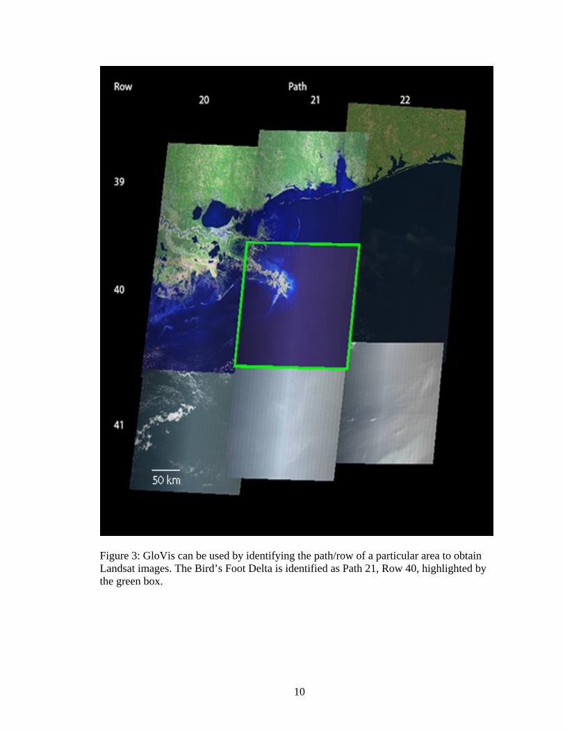
The Bird’s Foot Delta can be identified by using the path/row combination 21/40.
Using the USGS Global Visualization Viewer (GloVis), it is possible to pinpoint images
based on either their path/row, or latitude/longitude coordinates. A full-size image
downloaded from GloVis does not provide the highest quality image, due to the
30m/pixel resolution. The Head of Passes, represented by the highlighted box in Figure 3,
is seen in a full area Landsat image in Figure 4.
10
Figure 3: GloVis can be used by identifying the path/row of a particular area to obtain Landsat images. The Bird’s Foot Delta is identified as Path 21, Row 40, highlighted by the green box.
11
Figure 4: This image represents the full area of coverage seen in a single Landsat image obtained from GloVis (Path 21, Row 40) on October 29, 2009. The image covers a wide area (~85 km), with each pixel representing 30 m.
It is important to consider the size of the area being studied, and the range of the
images. The Landsat images encompass a snapshot of a path/row, of which I am studying
a small portion. As seen in Figure 5, the areas of interest indicated by the two boxes are
small areas in the Landsat image.
12
Figure 5: Landsat OLI image of the Head of Passes with four sub-areas investigated in this study highlighted in red boxes: (a) Yellow Cotton Bay (b) Zinzin Bay (c) North Mud Lumps (d) Port Eads. (e) Indicates a close-up area of the Head of Passes. See Fig. 9 for enlargements of these areas. (Image acquired April 23, 2016).
Another satellite database accessed was Google Earth. Google Earth is an easy to
use application, which contains a conglomerate of images taken from various sources.
Digital Globe, TerraMetrics and Spot Image are some of the satellite operators that
provide data to Google Earth. Landsat images are used as a base in Google Earth.
Although Landsat images have a resolution of 30 m, images found on Google Earth have
a resolution up to 2.5 m per pixel for color images and ~1.0 m/pixel for black and white.
This higher resolution allows smaller changes to be observed, and is used when possible.
13
However, these high-resolution images are not used as the primary dataset because they
have fewer images over a longer time scale.
2.1.1 Landsat Image Availability
Obtaining the data of images available for the region of interest was tedious, as
each image had to be observed, and chosen for comparison. Finding images that were
clear enough visually, and had comparable conditions was extremely important in this
Figure 6 displays the number of Landsat images available for each area of interest
by year. The Head of Passes, Atchafalaya Delta, Lafourche Delta, Mobile, and New
14
Orleans are the five areas highlighted in this study. The total number of images available
vary from 3066 (New Orleans), to 5944 (Lafourche Delta). This difference is due to the
path and rows of the location in question. Using the Landsatlook viewer, the area that is
identified as Lafourche Delta is displayed using four different path/row combinations.
Path 22 row 39, path 22 row 40, path 23 row 39, and path 23 row 40 are all represented in
an image mosaic when looking at one area on a 1:289 km scale. The Atchafalaya Delta is
also represented by four path/row combinations, while Mobile and the Head of Passes are
represented by three combinations. New Orleans only has two path/row combinations,
that cover the image area, which results in the lower total of images available.
2.1.2 Cloud-free Images
Although there are several thousand images available for each area, there are
significant fewer images that are pertinent to this study. The images are automatically
collected whether there are no clouds (0% clouds), total cloud cover (100% clouds) or
somewhere in between. When using the Landsatlook viewer, the default settings provide
a search with 20% cloud cover which drastically reduces the amount of time needed to
find suitable images. However, the low cloud cover does not necessarily mean that the
area being observed is visible, as a cloud may be over the exact area of interest with the
rest of the image cloud-free or visible (Figure 7 (Left)).
15
Figure 7: Close-up images displaying cloud cover of Fig. 5e, the Bird’s Foot Delta. (Left) Landsat TM image with a cloud cover of 11%, with clouds covering the exact areas of interest (Acquired October 2, 2005). (Right) Landsat OLI image with 40% cloud cover, but one area of interest is cloud-free. (Acquired May 23, 2015).
Alternatively, there are images at 40% cloud cover that have the area of interest
exposed, and are useful (Figure 7 (Right)). Of the two study areas observed in the image,
one is clearly seen, and one is covered by clouds. The comparison in Fig. 7 is helpful in
identifying parameters that may not be considered otherwise. Images with low cloud
cover percentages may be bypassed in favor of better quality images. However, images
with high cloud cover that are still usable are not considered at all if using cloud cover
percentage at a lower set value.
Another scenario in which high cloud cover percentage can be misleading is in
Figure 8. Here, there is a high percentage of cloud cover (29%), but all clouds are over
the water, with no clouds over the delta or areas of interest. The default cloud cover in
16
Landsat is 20%, and in most cases this limit is a good way to quickly identify useful
images.
Figure 8: Full area of coverage of Path 21, Row 40 Landsat SLC-off image with 29% cloud cover, no clouds over land. (Acquired April 7, 2007).
However, Figures 7-8 are good examples in displaying that there is value in
inspecting images that have varying cloud cover. The only way to truly filter through the
large database of images available is to look at each image individually, which is
extremely time consuming.
17
2.2 Determining Comparison Parameters
Accessing Mobile Geographics datasets was crucial in determining what images
should be compared (Mobile Geographics 2016). Satellite images are taken at the same
time at each location, so it is possible to determine the tide in the image. The tide and
currents website lists tide gauge locations, with multiple locations in Louisiana. The Head
of Passes gauge is located on the Bird Foot Delta, where the Mississippi River branches
in three directions. Mobile Geographics has tide data dating back to 1970, to the present,
providing a backlog of data. Nearby tide gauges show similar tides, and can be cross-
referenced if there are anomalous levels.
Comparing images is only possible if they are taken under similar conditions,
such as the stage of the tidal cycle. Approximately 60 Landsat scenes have been studied
over the nearly 30-year period of interest (1984-2016). By utilizing the tide data which I
obtained, it is possible to determine the tide when the image was captured. Images taken
at a certain tide can be compared at their respective high and low tides. Determining the
tides is important to get an accurate picture of what is occurring. An image at high tide
2compared to an image at low tide may give the impression that sea level is rising, even
though that may not be the case.
The tide data can be utilized by locating the time an image was taken, then finding
the height of the tide. Mobile Geographics graphs the tide on an x-axis of time, and a y-
axis of height. By finding the time on the x-axis, and the height on the y-axis, I can use
that tide as a reference for my image. Mobile Geographics also posts the heights of the
high and low tides, with the time. After analyzing and comparing the tide data of the
images, I was able to pick several images to compare each year.
18
It was extremely difficult finding images that had the same tidal levels at the same
time of day when the Landsat data were collected (e.g., 1.1m at 10:15). In order to use the
data collected, I had to look at the tide graphs from Mobile Geographics to observe the
pattern and compare images that had similar tidal heights and patterns.
Another factor in choosing images deals with the time of year, whether it was
daylight savings time, the season, an El Nino year, among other parameters. In regards to
this study, the main impact of El Nino on the Gulf of Mexico is increased precipitation
and flooding. Increased rainfall and flooding is relevant to this study because I am
observing where the shoreline is and tracing the water line.
In my data, I chose to compare the times in Central Daylight Savings Time (CDT)
as opposed to Central Standard Time (CST), simply because CDT lasts longer throughout
the year. Choosing either one does not matter, one was chosen at random to keep the data
consistent.
2.3 Comparing Images
Images that were considered comparable based on the previous sections
parameters were compared in Adobe Photoshop 2015. Initially, two images of similar
tides were compared in Photoshop by creating each image as its’ own layer. By
comparing images on top of each other, I changed the opacity of the top layer, and traced
the shoreline of the bottom layer. By tracing the shorelines onto the image of another day,
I was able to see if there were any changes over time.
Side by side comparison was also conducted in my study. After selecting
comparable images, I aligned the images next to each other and used lines, boxes, and
19
arrows to pinpoint areas on both images to present my data. The actual alignment was
done as stated in the previous paragraph, with layering one image on top of another. It is
much easier to display the data side by side for aesthetic reasons.
2.4 Tides
Tide data is extremely important in setting comparison parameters for this study.
Besides using tide data to set parameters, studying tide data can help to show changes on
a smaller scale. Mobile Geographics tide data highlights low and high tides, sunrise and
sunset, as well as moon cycles. Though not directly relevant to the goal of determining
sea level rise, these data are valuable in understanding the area of interest.
As observed in the SRTM data (Fig. 2), there are a significant amount of low-
lying areas in the delta complex. These low elevations are easily susceptible to changes in
sea level, tides, and flooding. Though other areas may experience much more intense
tidal cycles, the vulnerability of this location makes the tide data important in a different
way.
2.5 Gathering Data From Image Comparison
After comparing images in Photoshop, I was able to utilize the data by comparing
data side by side, pixel by pixel. By doing this comparison in Photoshop, I gained a
unique perspective in seeing the physical differences over small and large time periods,
by doing several time series over the entire area, as well as in specific areas. Although
this method is not useful in obtaining specific data as measuring distances and areas on
20
the ground, I was able to gain a general overview of the changes occurring in this region.
This is important, as I am not able to access the physical area to make my observations.
3.0 RESULTS
The main region of my study is the Mississippi Delta in Louisiana. Within this
region, there are three major study sites (Fig. 2): Lafourche Complex, Orleans Parish, and
Bird’s Foot Delta. The Lafourche Delta (Fig. 1) is no longer a river output, though it
contains areas of interest. Atchafalaya Bay was part of the Lafourche Delta, though it is
now recognized as part of the Atchafalaya Delta. For the purposes of this study, I identify
it as part of the Lafourche Delta and group it as such. Within these study sites, I looked
further into specific areas to identify changes.
3.1 Bird’s Foot Delta
Bird’s Foot Delta, also known as the Head of Passes (at the point where the river
meets the bay), is located in the Plaquemines Delta (Fig. 1). In Bird’s Foot Delta (Fig. 5),
the pinpointed areas I did an in-depth comparison were (Fig. 9): (a) Yellow Cotton Bay,
(b) Zinzin Bay, (c) North Mud Lumps, and (d) Port Eads. A twenty-five year time series
was studied for these areas, with particular attention to changes in the mid-2000s.
21
Figure 9: This site comparison includes images collected in 1995 (left), and 2016 (right). (a) Yellow Cotton Bay, near the beginning of Bird’s Foot Delta, has an intricate web of land and islands. (b) Zinzin Bay is a relatively sheltered area on the west side of the delta. (c) North Mud Lumps are located off the North Pass, extending the easternmost point of the delta. (d) Port Eads is located off the south branch of the Mississippi estuary, between East Bay and Garden Island Bay. See Fig. 5 for subscene locations.
22
3.1.1 Yellow Cotton Bay
Yellow Cotton Bay (Fig. 9a) had an area of approximately 12km2 disappear
between 1995 and 2016. There were also some areas that appear to be reinforced,
occurring naturally or human-engineered. Throughout the year 2003, changes were
observed, both an increase and a decline in land mass above water as indicated by arrows
(Figure 10). This could be due to tidal changes, as this area is more susceptible to smaller
changes in water height. At the time both images were collected, the tide was neither high
nor low, it was in between peaks, rising from a low tide. Figure 10 (Right) was closer to a
low tide than Figure 10 (Left), though the difference would not have been more than
0.2ft. An increase of approximately 0.2 km2 is observed in a land mass between May and
August of 2004 (Fig. 11 (top), (middle)).
Figure 10: These images of Yellow Cotton Bay (Fig. 9a) show increases and decline in land mass over a year. (Top) Acquired January 14, 2003 by TM sensor. (Bottom) Acquired November 14, 2003 by TM sensor.
23
Figure 11: These images of Yellow Cotton Bay (Fig. 9a) demonstrate land changes during 2004. (Top) Acquired May 24, 2004 by TM sensor, with 20% cloud cover. (Bottom) Acquired August 3, 2004 by TM sensor.
24
The SRTM data (Fig. 2) was collected in 2001, and Yellow Cotton Bay has the
darkest shading representing lowest topography of the four locations in Bird’s Foot Delta.
These low-lying areas decreased, and more water was observed of an area of
approximately 1 km2 over the course of the year.
Hurricane Katrina occurred in August 2005. Examining images available
immediately before (August) and after (September) the storm show significant
differences (Fig. 12). The small island or mass on the right side of the image disappears
in the September image. Another small mass, approximately 1 km2 also disappears. The
long bank on the right side of the image, running parallel to the river, appears to have
flooded almost completely through. There is an approximately 0.25 km2 decrease in
shoreline along the entire stretch of land on the left side of the image. Each of the areas
that disappeared between the August and September images are identified in dark green
on the SRTM image, except for the embankment. Though the embankment was not
identified as a low-lying area, it has water on both sides, storm damage and flooding from
the hurricane could explain why it did not stay the same.
Figure 12: Yellow Cotton Bay (Fig. 9a) shortly before and after Hurricane Katrina. (Left) Acquired August 22, 2005 by TM sensor with 20% cloud cover. (Right) Acquired September 16, 2005 by TM sensor.
25
Insignificant changes seen in images not shown in this paper could be due to tidal
changes and sediment movement.
3.1.2 Zinzin Bay
Zinzin Bay (Fig. 9b) proved to be an interesting case, as there appeared to be
increases in land area, and an appearance of small islands. Zinzin Bay is the most
sheltered of these four locations, and is most likely less impacted by storms and other
weather events. The bay is large and does not have a lot of land mass within it. There is
little change, though gradual increases in area during 2004, though the gains are absent in
October 2004.
Zinzin Bay is not particularly low-lying, as it is indicated in a slightly dark green
in the SRTM data, more comparable to North Mud Lumps than the closer upstream
Yellow Cotton Bay. Cloud cover and discoloration made this area somewhat difficult to
observe.
Images observed immediately before and after Hurricane Katrina, which made
landfall August 23, 2005 show some changes (Fig. 13), though not significant ones as
seen in other study sites. The loss of land appears to be sediment, or the other changing
mass as seen in early 2004. The protectiveness of the bay appeared to have shielded this
area from extreme change or flooding during the hurricane.
26
Figure 13: Zinzin Bay shortly before and after Hurricane Katrina (top) Acquired August 15, 2005 by the TM sensor. (bottom) Acquired September 15, 2005 by the TM sensor. See Fig. 9b for location.
27
February 2010 marks the first appearance of the long, straight land masses
(approximately 1.45 km long) (Fig. 14a). The mass was joined by two larger masses
stretching nearly 2km long in the summer of 2013 (Fig. 14b), exactly when is difficult to
pinpoint due to high cloud cover. The initial mass began to shrink in 2014 (Fig 14c), and
another mass appeared in 2015 (Fig 14d).
Figure 14: Appearance of land masses in Zinzin Bay. (a) Acquired February 2, 2010 from the TM sensor. (b) Acquired July 28, 2013 from the ETM-off sensor. (c) Acquired October 11, 2014 from the OLI sensor. (d) Acquired June 8, 2015 from the OLI sensor with 25% cloud cover. See Fig. 9b for location.
28
3.1.3 North Mud Lumps
Within North Mud Lumps, dramatic change is observed between 1997 and 2004.
In 1995 (Fig. 9c (left)), there is a y-shaped offshoot where water flows, yet the bottom
portion can no longer be seen in 2016 (Fig. 9c (right)). When studying images on Google
Earth, the main time period of gradual land loss occurs between 1997 and 2004.
Figure 15: This pair of images of the North Mud Lumps was collected shortly before and after Hurricane Katrina. (Left) Acquired August 15, 2005 by the TM sensor with 7% cloud cover. (Right) Acquired September 16, 2005 by the TM sensor with 0% cloud cover. See Fig. 9c for location.
29
Figure 16: Disappearance of the bottom y-shaped in the North Mud Lumps between November 2005 and February 2006. (Left) Acquired November 19, 2005 by the TM sensor with 10% cloud cover. (Right) Acquired February 7, 2006 by the TM sensor with 18% cloud cover. See Fig. 9c for location.
Before and after images in August and September of 2005 (Fig. 15) show land
changes that can be attributed to Hurricane Katrina. What appeared to be a small barrier
near the tip of the upper y-shape is no longer there in September. Accelerated decrease in
area of the bottom y-shape occurred as well. By November 2005 (Fig. 16, left), nearly the
entire bottom portion disappeared, and by February 2006 (Fig. 16, right), there is no trace
of it.
3.1.4 Port Eads
Port Eads (Fig. 9d) is the area of the middle offshoot of the Mississippi River,
bordered by East Bay on the left, and Garden Island Bay on the right. This area does not
have good SRTM data, as the image is partially cut off. However, what is represented in
the SRTM data shows that this area is not particularly low, indicated by the bright green
color. Though this area is not as susceptible to sea level rise as its’ surroundings, Port
Eads is interesting to look at due to the dramatic changes that can be seen at a distance.
30
Figure 17: These images from 1995 and 2016 show significant changes in Port Eads. The red rectangles identify the land changes. (Left) Acquired April 15, 1995 by TM sensor. (Right) Acquired April 23, 2016 by TM sensor. See Fig. 9d for location.
Port Eads has dramatic changes occurring between 1995 and 2016 (Fig. 17). The
area indicated by the red box in 1995 (Fig. 17 (left)) completely disappears by 2016 (Fig.
17 (right)), as a new stretch of land appears almost perpendicular to the original area. The
disappearance and addition of land occurs simultaneously, seen in Google Earth images.
The images indicate the small parcel of land disappears around 2006 (Fig. 18 (right)).
The end of the land appears to have shifted about 20 degrees up from where the river
ends. This is most likely an example of longshore drift, with sediment naturally moving
due to ocean currents.
31
Figure 18: These images show intermediate changes of Port Eads at low tide (Left) Acquired February 9, 2001 by TM sensor. (Right) Acquired February 7, 2006. See Fig. 9d for location.
Comparing images from August and September of 2005 (Fig. 19), there is not
much change in area that I am observing. There is much change further up the river, on
the east side. The area, which had relatively little change before, experienced significant
change after Katrina, due to either flooding or direct impact from the storm.
Figure 19: Port Eads shortly before (Left) August 15, 2005 and after (Right) September 16, 2005 Hurricane Katrina. See Fig. 9d for location.
32
3.2 Miscellaneous Islands
There are many miscellaneous islands along the Louisiana coastline. Some islands
stood out and warranted further research. These islands were chosen due to their
vulnerability, observed change in a preliminary time-series, and known anthropogenic
impacts. Shell Island, Isles Dernieres, and Isle de Jean Charles stood out and were chosen
as additional study sites.
Shell Island, in Vermilion Bay, is considered part of the previous Teche Delta
Complex (Fig. 1). This island is different from the others in this section because it was
the focus of anthropogenic reconstruction. Sediment from the Mississippi River was used
to restore the barrier island, as opposed to natural phenomena such as longshore drift.
Isles Dernieres is a part of the Lafourche Delta Complex, also highlighted in Fig. 1.
Although the SRTM data do not extend to where the Atchafalaya meets the Gulf
of Mexico, there are portions of the SRTM data that are still useful. Section 3.2.2. focuses
on Isles Dernieres, which can be seen in the SRTM data (Fig. 2b). Fig. 20 provides a map
indicating the location of Shell Island (Fig. 21), that is not seen in the SRTM data.
33
Figure 20: This image from Google Earth covers the same area as Fig. 1, with Fig. 21 highlighted in the red rectangle.
3.2.1 Shell Island
Shell Island is located near the end of the Lower Atchafalaya River. A small
island of little more than 6.48 km2, there are several other islands and landforms in the
vicinity. The Shell Island location had some loss and gain in land area. In the lower
portion of the area, there was sediment accretion, while the upper portion experienced a
slight decrease in area. Shell Island was the product of man-made restoration efforts.
Sand was dredged from the Mississippi River to reconstruct the island.
34
Figure 21: Shell Island images acquired from Google Earth (top) December 30, 1984 (middle) December 30, 1995 (bottom) December 30, 2016.
35
In 1984, there was little to no extended area above the Shell Island Pass. An area
~2.6 km2 appeared later, by 1995. Small forms encompassing ~3.9 km2 shifted downward
compared to the map on LandsatLook. From 1993 to 1995 there was an appearance of
small 0.65 km2 islands or masses to the southwest of Shell Island. These appear to be
affected by sediment deposition, as you can see the path of sediment from the end of
larger masses to the smaller masses.
3.2.2 Isles Dernieres
Isles Dernieres is a group of islands with a land area of ~7.5 km2 as of 2017, south
of Lake Pelto, indicated by the red box in Fig. 22. Originally a 110 km2 barrier island,
Isle Derniere (Last Island) was destroyed in the 1856 Last Island hurricane. The
remaining portions of the island are identified as Racoon Island, Whiskey Island, Trinity
Island, and East Island. Isles Dernieres marks the southern boundary of the state and
appears to act as a barrier, protecting the inner low-lying islands. As observed in the
SRTM data, this island is indicated in dark green, a low-lying area. As this island is at a
low elevation, and looks like a protective boundary, the island is important to the area, as
well as this study. There was no significant change observed in Isles Dernieres
immediately after Hurricane Katrina.
36
Figure 22: Map of Atchafalaya Delta, with Isle Dernieres (Fig. 23) indicated in the red rectangle. (Acquired November 3, 2014). See Fig. 2b for location.
Figure 23: Isles Dernieres 1994-2016 comparison. (top) Acquired September 24, 1994. (bottom) Acquired December 10, 2016.
37
3.2.3 Isle de Jean Charles
Isle de Jean Charles is an interesting case, as it is difficult to observe with satellite
data. Though this location proved to be a challenge for this study, the importance of
studying this location should not be understated. An important location culturally, this
small island is home to indigenous people who were displaced by the Indian Removal
Act, and the Trail of Tears. The people lived off the resources provided by the ocean, and
levees destroyed the natural marshland. This area is difficult to obtain satellite data for, as
the island is only 0.25 miles wide, having lost 98% of its land mass since 1955
(Lagamayo, 2017).
3.3 Orleans Parish
An important region in my study is the Orleans parish, and the city of New
Orleans. A densely populated area, this major U.S. port is the largest city and
metropolitan area in the state. Portions of the Orleans parish are below sea level, there are
various environmental threats to the area. Although the city is protected by levees and
other engineering efforts, there was still extensive flooding during Hurricane Katrina. Big
Branch Marsh National Wildlife Refuge and Lake St. Catherine are two areas on different
sides of Lake Pontchartrain that were affected differently by both Hurricane Katrina as
well as sea level rise.
38
Figure 24: Map of Lake Pontchartrain with areas of interest highlighted. Red boxes show locations of Figs. 25, 28, and 30. (a) Big Branch Marsh National Wildlife Refuge (Fig. 25). (b) Lake St. Catherine (Fig. 28). (c) New Orleans (Fig 30). See Fig. 2a for location.
3.3.1 Big Branch Marsh National Wildlife Refuge
The Big Branch Marsh National Wildlife Refuge is located on the north side of
Lake Pontchartrain (Fig. 24a). In the SRTM data (Fig. 2), the refuge is indicated in dark
green, with very low elevation. In addition, there are no seawalls or barriers guarding the
shoreline from the water. This is important for the purposes of my study because it is
possible to see direct impacts of shoreline change without the interference of seawalls or
other anthropogenic barriers.
Efforts to restore the marsh include pumping sediment from Lake Pontchartrain to
create low salinity brackish marsh in current open water ponds (U.S. Department of the
Interior, 2007). As seen in Figure 25, there are several areas that gained sediment, and
39
others that lost sediment. Purposeful movement of sediment is one reason for changes, as
well as rising sea level.
Figure 25: Big Branch Marsh National Wildlife Refuge (top) TM image acquired from Landsat June 10, 1996. (bottom) OLI image acquired from Landsat December 10, 2016. This twenty-year comparison shows different areas flooding and gaining sediment. See Fig. 24a for location.
40
Figure 26: Big Branch, the same area as Fig. 24a (top) TM image acquired by Landsat August 22, 2005. (bottom) TM image acquired by Landsat September 7, 2005. This pair of images shows areas that were flooded immediately after Hurricane Katrina.
Comparing August to September 2005 (Fig. 26) highlights flooding and damage
inflicted by Hurricane Katrina. An area of water ~0.65 km2 appeared in the bayou in
September 2005. Instead of decreasing in area with time, as other flooded areas did, the
41
area covered by water expanded until October 2008. Water began receding in November
2008 and stayed at that level, will little fluctuation until summer of 2015, where the water
level appeared to decrease again.
Figure 27: Big Branch (top) TM image acquired by Landsat on November 2, 2008. (bottom) TM image acquired December 8, 2015. These images show decreases in flooded areas from 2005. See Fig. 24a for location.
42
3.3.2 Lake St. Catherine
Lake St. Catherine is located to the east of the Orleans Parish, north of the Lake
St. Catherine Gas Field (Fig. 24b). The Lake St. Catherine Gas Field resides on Bayou
Sauvage National Wildlife Refuge, the largest urban wildlife refuge in the United States.
This particular location is a gas field on a national wildlife refuge, and though the
shorelines are not important in protecting citizens’ property, it is still important for the
wildlife living there.
This 11-year time series is represented by images with the same tide levels.
Examining images from 2005 to 2016, there are some distinct changes in shoreline and in
the field (Fig. 28). Changes in the shoreline, as well as previously aboveground areas that
flooded are highlights of this location. As seen in Figure 28, both the arrows on the left,
as well as the ones in the center point out areas that appear to have flooded. The arrow on
the right points out the jagged edge of the shoreline, which looks different in 2016 from
2001.
43
Figure 28: Lake St. Catherine (top) TM image acquired by Landsat November 15, 2001. (bottom) TM image acquired by Landsat November 17, 2016. The arrows indicated in both images draw attention to changes in the shoreline. See Fig. 24b for location.
Comparing images from August to September of 2005 there was much flooding
observed in the field, and breaks in the shoreline. Much of the flooding in the middle of
the field eventually dissipated, although the breaks in shoreline were not repaired, giving
some areas a ragged appearance. Images from 2016 show the flooded areas caused by
Hurricane Katrina were not lasting, but the damage to the shoreline was.
44
Figure 29: Lake St. Catherine (top) TM image acquired by Landsat August 22, 2005. (bottom) TM image acquired by Landsat September 7, 2005. This pair of images shows the large amounts of flooding immediately post-Katrina. See Fig. 24b for location.
45
3.3.3 New Orleans
The actual city of New Orleans (Fig. 24c) is protected by man-made boundaries.
However, Hurricane Katrina was able to break through the protections and flood the city.
This technical failure warrants examining the city and observing pre- and post- Katrina
impacts. Images taken shortly before and after the storm hit, as well as images from a few
months after the storm and over a decade later can give some insight into changes and
recovery in this area.
New Orleans flooded during Hurricane Katrina not due solely to the storm, rather
the lack of effective infrastructure and poor planning. As seen in the middle image of
Figure 30, the widespread flooding indicated in blue affected large portions of the city.
Although Katrina was a major disaster, the long term impact on the geography of the land
was not as long lasting as the socioeconomic impact. The bottom image of Figure 30
shows that the city was able to recover from flooding, but there were minor changes still
seen at the satellite level. The main waterways look relatively unchanged.
46
Figure 30: New Orleans (top) TM image acquired from Landsat August 22, 2005. (middle) TM image acquired from Landsat September 7, 2005. (bottom) TM image acquired from Landsat October 25, 2005. These images are compared to visualize the massive flooding in the city. See Fig. 24c for location.
47
Examining the failure of flood walls and levees in the event of Hurricane Katrina
is significant, as technological innovations affect the impact of natural disasters. Most
locations in my study do not have any walls to prevent flooding or bar against sea level
rise. Being able to compare a highly engineered effort to a natural shoreline allows
critique of how to handle the issues of sea level rise and climate change. The complexity
of New Orleans and Hurricane Katrina has been, and needs to be studied and dealt with
on a large physical, social and economic platform, as opposed to a strictly physical level
in building seawalls.
3.4 Shoreline Image Comparison
After comparing images in the Bird’s Foot Delta over a timespan of nearly 40
years, there are several significant changes in the area. The time-series seen in the
previous sections show that the method of my study is successful in comparing
shorelines. The shoreline changes are easy to see, though determining whether the
changes are sea level rise is difficult. Landsat provides a wealth of data, though early
images from the first satellites are most useful as providing a before and after contrast as
opposed to using them to analyze changes. Figure 31 shows a 33-year comparison of
Bird’s Foot Delta.
Shoreline comparison is relevant and important because even if sea level rise is
not determinable, sinking land still affects the delta. Previously accessible areas may no
longer be accessible, or usable, and it is important to identify the areas.
48
Figure 31: Bird’s Foot Delta (top) MSS image acquired January 15, 1983. (bottom) TM image acquired April 23, 2016.
49
4.0 DISCUSSION
The implications of my results can reveal important concerns about the future of
the Mississippi Delta, and other low-laying coastal areas. By observing the patterns of the
past, and use current data and models to predict the future, we can plan accordingly.
Observing the high-risk areas is important in preserving natural environments, people,
and personal property.
4.1 Difficulties in Using Tide Data
Finding tide data associated with the area of interest was quite difficult. NOAA
has a handy tides and currents website that has data for Pilottown, LA, the area of interest
(https://tidesandcurrents.noaa.gov/waterlevels.html?id=8760721). However, there is a
distinct lack of historical confirmed tide data available. There are confirmed water levels
from September 2011 to the present.
To substitute for the lack of confirmed data, I used tide predictions from Mobile
Geographics referencing the Head of Passes, Mississippi River
(http://tides.mobilegeographics.com/locations/2484.html). I was able to do this with
confidence because the verified tides found on the NOAA website follow the same trend
as the predicted tides, though not the actual heights. For example, if the tides have a
consistent 0.5 ft discrepancy from the actual tide height, the general low/high pattern is
still followed.
50
4.2 Results Analysis
The red boxes seen in Figure 2 may seem arbitrary, however they correspond to
the view of images on the LandsatLookViewer. The SRTM data are extremely important
to my study, and using they provide a base map for identifying areas of low and high
ground. The red boxes identified areas of low elevation, which were studied in detail in
the smaller scale sites. The 2001 SRTM data suggested future loss in Isles Dernieres (Fig.
23) and Lake St. Catherine (Fig. 28), where the dark areas corresponded to low areas.
Figure 10 is a good example to highlight for small tidal changes. Though the tides
in both images are lower (though not low) tide, there are areas that appear different.
These changes are on the meter level, less than a kilometer. Another challenge in
analyzing those images is to determine what is discoloration of sediment by the Landsat
“Natural Look” image, or actual exposed land. The discoloration makes the image appear
to have larger or extended land mass, and it is difficult to differentiate between the two.
Figure 14 is an example of an event that is neither subsidence nor sea level rise.
This area showed a gain in area as opposed to loss suggested by low ground in the SRTM
data. These unique masses appear and move over a five-year period. The rate of increase
of land area is approximately 1km per year. These changes appear to be due to unnatural
causes, sediment deposition affected by human activity, as there are no significant
changes in the coastline, so the changes are coming from a different source.
I found it important to use Hurricane Katrina as a reference point in this study
because it was an impactful event physically, socially, and economically. For the
purposes of this study, the physical events are most relevant, but the socio-economic
status of the area affected the impact of the hurricane. One of the most significant sites to
51
compare pre- and post- Katrina was New Orleans. In New Orleans, Hurricane Katrina
was able to break through protections and flood the city. This technical failure warranted
examining the city and observing pre- and post- Katrina impacts. Observing part of the
city in August 2005, at the bottom of the image near the river there are approximately 10
dark spots that can be pinpointed. In September 2005, the amount of dark spots nearly
doubled and dark blue areas can be observed in and around the city. Initially, I thought
the dark spots could be flooding, but after comparing images to Google Maps and Google
Earth, I determined them to be shadows from tall buildings. Increases in following years
can be attributed to construction of tall buildings, confirmed on Google Maps.
4.3 Use of These Methods to Observe Temporal Changes
This method a useful tool in studying temporal changes, with the wealth of data
available. One aim of this project is to use the satellite data to observe sea level rise,
though this project would need to be expanded on to do so. Using this method of satellite
images and tide data to determine sea level rise is a rather tedious process, and may not
be the best method to quantify specific amounts of change. Conducting a time-series of
images of similar tides is helpful to give an overview of the changes that occur over the
timespan, but it requires additional research to determine when the changes occurred.
Gaps in usable data cannot be helped, as the weather conditions of the area are not able to
be accommodated by the satellite taking images.
Combining several datasets to gain a full picture of the area of study was done by
not only comparing areas with similar tides, but examining images over the study area
taken on the same day. This was easier to do in Bird’s Foot Delta, as the entire delta is
52
seen during one row/path, allowing the entire delta to be compared using the same image.
This is important in understanding whether the changes seen in the time-series are due to
tides or sea level rise, if it is uniform across the entire study area, it could be sea level
rise.
4.4 Future Research
This project can be expanded in several aspects: comparing additional locations,
examining longer time-series, using same method in different locations. In this study, I
compared three different areas, and examined specific areas in each. In the future, more
sites in the general area could be studied, or a study of the entire delta, perhaps dividing
the area systemically and researching individual blocks of area. Areas such as Mobile,
Alabama were considered for this study and data was gathered, but were ultimately
dismissed for this study. These areas could be ones explored in the future.
This method could be used in other areas, and coupled with other resources
available. Using GIS or other programs can help to determine quantifiable changes, and
expand on these results. Areas at high risk of sea level rise such as Bangladesh may
benefit from similar studies. However, it is crucial to have tidal data available to
confidently compare satellite images.
53
5.0 CONCLUSION
This purpose of this study was to determine if this method is a viable option to
observe sea level rise in the Mississippi Delta. The results showed that we can observe
shoreline changes and sea level rise, though not in a definite quantifiable manner. Time-
series over the span of over twenty years, as well as over the course of a single year can
be conducted and show changes. This method can be used to successfully determine
when the changes occurred, generally within a month.
Changes in shoreline in the Mississippi Delta are due to several factors: sea level
rise, human infrastructure, ground subsidence, and natural shoreline drift due to changes
in the discharge of sediment from the delta. Some areas explored in this study were
impacted by all of these factors, others had one or two in play.
The amount of change seen in this region is generally on the kilometer scale, or
less. Land disappears and appears in areas of 1 km or more, while flooding and other
shoreline changes are smaller, seen in a few pixels in the range of 50-100s of meters. This
range of sizes is significant because the larger changes seen appear to be due to forces
other than sea level rise. These large changes are due to storms, human construction, and
longshore drift. The areas that change on a smaller scale are more likely due to sea level
rise, as the images are taken at the same point in the tidal cycle. These smaller changes
are not unimportant, as major events can exacerbate the changes.
In certain study sites Hurricane Katrina was the main factor in changing
shorelines. Regardless of the impact of the storm in each area, I found it valuable to
compare images shortly before and after the storm for each of the study areas. Areas
around Lake Pontchartrain (Figs. 29 and 30) saw major impacts where the storm caused
54
breaks in levees and mass flooding. Observing the storm’s impact through satellite
images is useful because it can be used to track further changes in this area as well as
other areas. The long-term effects of Hurricane Katrina are also observed in this study.
Flooding and some changes are to be expected from a large-scale storm, though there did
not seem to be many long term-impacts. Within the Bird Foot Delta study sites, Port Eads
experienced flooding parallel to the Mississippi River can be observed in satellite images
as well. Major flooding that occurred in New Orleans (Fig. 30) is observed to have
dissipated within about a month (Fig. 30). Variability in areas before and after the storm
can give accountability to changes from the storm. for about 6 km (Fig. 19). When
observing images of this area in 2016 (Fig. 17), the land has not recovered, showing that
Katrina had a major role in changing the geography of this area. In the North Mud
Lumps, the “y-shaped offshoot” was not significantly impacted by Katrina, yet major
changes were seen within the year following the storm. This implies that major storms
may not have an immediate impact on areas, but can change variability in the future.
The SRTM data is useful in predicting areas of change, though not necessarily
flooding. One small area (~12 km2) of New Orleans was indicated at a low elevation,
though a much larger area (100 km2) was flooded during Hurricane Katrina. Images
observed after flooding receded did not show further changes in this area. The SRTM
data are useful, but should not be used alone. A helpful tool, it should be coupled with
weather conditions, tide data, or other resources to see a clearer picture of the area in
question. The SRTM data were useful in this study because I paired it with tide data in
the process of selecting images, other satellite images, and knowledge of major weather
events (Hurricane Katrina).
55
Going into this study, a major question is whether changes were due to sea level
rise, land subsidence, or changes in the discharge rate of sediment from the Mississippi
River. In areas such as Port Eads (Fig 23), changes in sediment deposition caused
dramatic changes to appear, neither sea level rise nor subsidence. Though these two
examples do not help to answer this particular question, they shed insight on some of the
behavior in this area. Images of Port Eads can show where the sediment is moving to and
from, and Shell Island shows the efforts of humans building artificial islands. Both sea
level rise and land subsidence can be seen in this study, with land subsidence in areas
such as New Orleans and near the Atchafalaya Delta. Previous studies (Yu et.al 2012)
show that Holocene sediment loading of marsh basal peat in these areas. However, in the
Bird’s Foot Delta and Isle Dernieres, there are differences in rates and amount of change.
These differences lead to the conclusion that these other areas are experiencing sea level
rise as opposed to land subsidence.
This study is relevant, as sea level rise and the impacts of climate change are seen
worldwide. Areas such as Bangladesh are highly susceptible to sea level rise and
flooding, using the Mississippi Delta is a good test to see if it is applicable to other areas.
Low-laying coastal areas that need attention, but are not easy to access or measure from
the ground can benefit from the use of satellite images and SRTM data.
56
LITERATURE CITED
Allen, Yvonne C., Brady R. Couvillion, and John A. Barras. 2011. “Using Multitemporal
Remote Sensing Imagery and Inundation Measures to Improve Land Change Estimates in Coastal Wetlands.” Estuaries and Coasts 35 (1): 190–200. doi:10.1007/s12237-011-9437-z.
Blum, Michael D., and Harry H. Roberts. 2009. “Drowning of the Mississippi Delta due
to Insufficient Sediment Supply and Global Sea-Level Rise.” Nature Geoscience 2 (7): 488–91. doi:10.1038/ngeo553.
Coastal Wetlands Planning, Protection and Restoration Act. 2016. “The Mississippi River
Delta Basin.” Accessed March 18. http://lacoast.gov/new/about/basin_data/mr/default.aspx.
Ericson, Jason P., Charles J. Vörösmarty, S. Lawrence Dingman, Larry G. Ward, and Michel Meybeck. 2006. “Effective Sea-Level Rise and Deltas: Causes of Change and Human Dimension Implications.” Global and Planetary Change 50 (1–2): 63–82. doi:10.1016/j.gloplacha.2005.07.004.
Farr, T. G., and M. Kobrick. 2000. “Shuttle Radar Topographic Mission Produces a
Wealth of Data” Eos Trans AGU, 82, 583-585. Guinness World Records. 2016. “Longest-Operating Earth Observation Satellite.”
Guinness World Records. http://www.guinnessworldrecords.com/world-records/longest-operating-earth-observation-satellite.
Intergovernmental Panel on Climate Change. 2016. “Climate Change 2014 Synthesis
IPCC, 2014: Climate Change 2014: Synthesis Report. Contribution of Working Groups I,
II and III to the Fifth Assessment Report of the Intergovernmental Panel on Climate Change [Core Writing Team, R.K. Pachauri and L.A. Meyer (eds.)]. IPCC, Geneva, Switzerland, 151 pp.
Kappler, John. Mississippi Delta Formations. National Geographic Society. 2016.
NASA’s Landsat Education and Public Outreach team. 2006. “How Landsat Images Are
Made.” http://landsat.gsfc.nasa.gov/pdf_archive/How2make.pdf. Nevis, Sean. 2015. “Indigenous Louisiana Tribe Losing Their Land To Climate Change
Faster Than Anywhere In The World.” MintPressNews. http://www.mintpressnews.com/indigenous-louisiana-tribe-fighting-to-save-their-lands-from-climate-change/204811/
Palaseanu-Lovejoy, Monica, Christine Kranenburg, John A. Barras, and John C. Brock.
2013. “Land Loss Due to Recent Hurricanes in Coastal Louisiana, U.S.A.” Journal of Coastal Research, April, 97–109. doi:10.2112/SI63-009.1.
“SLC-off Products: Background.” 2016. Accessed March 16.
http://landsat.usgs.gov/products_slcoffbackground.php. US Department of the Interior, Fish and Wildlife Service. 2007. “Comprehensive
Conservation Plan Big Branch Marsh National Wildlife Refuge.” https://ecos.fws.gov/ServCat/DownloadFile/1365?Reference=1390
US Department of the Interior, USGS. 2015. “Landsat Missions Timeline.”
http://landsat.usgs.gov//about_mission_history.php. Visser, Nick. 2014. “Louisiana Is Drowning. Quickly.” The Huffington Post. August 28.