Using Spatial Econometrics to Assess the Impact of Swine Production on Residential Property Values Jungik Kim Ph.D. candidate Department of Urban Planning University of Illinois Peter Goldsmith Assistant Professor NSRL Endowed Fellow in Agricultural Strategy Department of Agricultural and Consumer Economics University of Illinois Michael Thomas Assistant Professor Department of Agribusiness Florida A&M University Presented as a Selected Paper at the annual meeting of the American Agricultural Economics Association, Denver, July, 2004 Contact author: Peter Goldsmith Email: [email protected]Telephone: (217) 333-5131 Fax: (217) 333-5538
Transcript
Using Spatial Econometrics to Assess the Impact of Swine Production on Residential Property Values
Jungik Kim PhD candidate
Department of Urban Planning University of Illinois
Peter Goldsmith
Assistant Professor NSRL Endowed Fellow in Agricultural Strategy
Department of Agricultural and Consumer Economics University of Illinois
Michael Thomas
Assistant Professor Department of Agribusiness
Florida AampM University
Presented as a Selected Paper at the annual meeting of the American Agricultural Economics Association Denver July 2004
Using Spatial Econometrics to Assess the Impact of Swine Production on Residential Property Values
Copyright 2004 by Jungik Kim and Peter Goldsmith and the University of Illinois BOT All rights reserved Readers may make verbatim copies of this document for non-commercial purposes by any means provided that this copyright notice appears on all such copies
1
Abstract A spatial hedonic model is developed to assess monetary harm of confined animal feeding
operations (CAFOs) on property values taking explicitly spatial dependence in property
values into account Spatial autocorrelation was found in the form of spatial lag dependence
not spatial error dependence When spatial lag dependence is explicitly taken into account on
average the impact is reduced by 18 The magnitude of the spatial autoregressive
parameter was about 02 for the 1-mile distance band meaning one-fifth of the house value
could be explained by the values of the neighboring houses
Key Words Spatial hedonics spatial autocorrelation spatial lag dependence spatial error
Using Spatial Econometrics to Assess the Impact of Swine Production on Residential Property Values
Copyright 2004 by Jungik Kim and Peter Goldsmith and the University of Illinois BOT All rights reserved Readers may make verbatim copies of this document for non-commercial purposes by any means provided that this copyright notice appears on all such copies
2
Introduction Hedonic models in housing and real estate have traditionally used housing physical attributes
and locational characteristics variables to estimate how a certain housing attribute marginally
contributes to housing price Examples of physical attributes variable include floor area the
number of rooms the number of bathrooms or house age For locational characteristics two
kinds of measures are commonly employed an accessibility measure such as distance to the
Central Business District (CBD) and a neighborhood indicator measure such as median
household income Housing values for example would be negatively associated with
distance to CBD due to increased transportation cost Similarly median household income
can be an indicator for neighborhood quality Hedonic models are also used to measure the
negative externality of a noxious facility such as a landfill or a hazardous waste site (see
Kohlhase Kiel and Zabel and Hite et al among others) Distance to such a facility is
additionally used as a locational variable to examine how the negative impacts of the facility
are a function of distance
Hedonic models using locational variables however do not fully account for spatial
autocorrelation in housing prices Spatial autocorrelation refers to the cluster of similar
values in space (Anselin and Bera) Housing prices are spatially autocorrelated because
neighborhood residential properties share location amenities such as public services (Dubin
Basu and Thibodeau) The boundaries of neighborhoods are not always clear-cut and the
objective measures of neighborhood quality are often difficult to obtain The residuals from
hedonic models are likely to be spatially autocorrelated OLS estimates then will be unbiased
but inefficient (Dubin Pace and Thibodeau) Spatial autocorrelation also arises from a
mismatch in spatial scale (Anselin and Bera) Two situations can be discerned First using
an indicator variable for neighborhood quality such as median income will induce a spatial
Using Spatial Econometrics to Assess the Impact of Swine Production on Residential Property Values
Copyright 2004 by Jungik Kim and Peter Goldsmith and the University of Illinois BOT All rights reserved Readers may make verbatim copies of this document for non-commercial purposes by any means provided that this copyright notice appears on all such copies
3
mismatch as the data is only available on the census tract or block-group level The spatial
scale of the census tract or block-group level is larger than that of an individual house
resulting in positive spatial autocorrelation Similarly in the case of a noxious facility and its
surrounding properties the negative impacts of the facility tend to spill across houses The
spatial scale of the impact is larger than an individual house and causes spatial
autocorrelation In the presence of spatial autocorrelation there is a loss of independent
observations The inclusion of a spatially lagged variable in the hedonic model addresses this
loss of information (Anselin and Bera)
The issue of spatial autocorrelation has received little attention in hedonic studies in rural
settings The purpose of this article is to advance the methodology of rural hedonic studies
by developing a spatial hedonic model that explicitly accounts for spatial autocorrelation in
housing prices in the assessment of the monetary harm of confined animal feeding
operations (CAFOs) on rural property values To date none of the existing studies on the
impact of swine operations on property values has addressed the issue of spatial
autocorrelation in housing prices1 This article will contribute to the literature by providing a
benchmark for future hedonic studies of rural land use
Literature Review
Spatial autocorrelation between spatial objects can be formally defined by the moment
condition as follows (Anselin and Bera p 241)
(1) 0][][][]cov[ nesdotminus= jijiji yEyEyyEyy for ji ne
where i j refer to individual locations and iy and jy denote the value of a random variable
at that location The covariance structure becomes spatial when nonzero i j pairs are
Using Spatial Econometrics to Assess the Impact of Swine Production on Residential Property Values
Copyright 2004 by Jungik Kim and Peter Goldsmith and the University of Illinois BOT All rights reserved Readers may make verbatim copies of this document for non-commercial purposes by any means provided that this copyright notice appears on all such copies
4
interpreted ldquoin terms of spatial structure spatial interaction or the spatial arrangement of the
observationsrdquo (Anselin 2001a p 312)
Two approaches direct and indirect representation are suggested in the literature to
model the covariance structure (Anselin 2001a) Direct representation adopted from a
geostatistical approach assumes a continuous surface and expresses spatial interaction as a
continuous function of distance In contrast an indirect representation or lattice approach
presumes that the spatial effect is a function of the interaction among discrete spatial objects
Although direct representation has been applied to real estate markets an indirect approach is
more suited to economic studies dealings with discrete objects in space such as counties or
regions (Anselin and Bera) Moreover specifications used in direct representation have
estimation and identification problems For example the nuisance parameter is not identified
under the null hypothesis resulting in a singular information matrix (Anselin 2001b)
Direct representation focuses on improving spatially autocorrelated residuals by directly
estimating the covariance structure (Dubin Basu and Thibodeau) Spatial covariance is
expressed as a smooth decay function of the distance between observations For example
Dubin specified the covariance structure as
(2) )exp( 21 bdbK ijij minus=
where ijd is the distance between the i and j th observations and 1b and 2b are parameters
to be estimated Basu and Thibodeau used a semivariogram to estimate the covariance
Using Spatial Econometrics to Assess the Impact of Swine Production on Residential Property Values
Copyright 2004 by Jungik Kim and Peter Goldsmith and the University of Illinois BOT All rights reserved Readers may make verbatim copies of this document for non-commercial purposes by any means provided that this copyright notice appears on all such copies
5
where is denotes location of an observation i and )( isξ denotes the hedonic residual for an
observation at is 2
In indirect representation the specification of a spatial process indirectly determines a
covariance structure which requires constructing a relevant spatial weights matrix In
indirect representation two types of spatial dependence spatial lag dependence and error
dependence are conventionally distinguished (Anselin 1988) Spatial lag dependence arises
from spatial interaction between economic agents such as counties or states or mismatch in
spatial scale Spatial lag dependence is modeled by incorporating a spatially lagged
dependent variable in hedonic models analogous to the inclusion of a serially autoregressive
term for the dependent variable ( 1minusty ) in a time-series context The inclusion of a spatial
lagged dependent variable has two implications (Anselin and Bera) First OLS estimates
will be biased and inconsistent because a spatially lagged dependent variable is endogenous
and always correlated with the error term Second the simultaneity must be explicitly
accounted for either in a maximum likelihood estimation framework or by using a proper set
of instrumental variables
On the other hand spatial error dependence arises from noise in the model and can be
specified as a spatial process for the disturbance term The effect of a spatial residual
autocorrelation on the OLS estimator is analogous to time-series results The OLS estimates
will be unbiased but inefficient More efficient estimators are obtained by specifying the
error covariance implied by the spatial process
Spatial Weights Matrix
The specification of a covariance structure in indirect representation requires constructing a
relevant spatial weights matrix The choice of spatial weights is made empirically in many
Using Spatial Econometrics to Assess the Impact of Swine Production on Residential Property Values
Copyright 2004 by Jungik Kim and Peter Goldsmith and the University of Illinois BOT All rights reserved Readers may make verbatim copies of this document for non-commercial purposes by any means provided that this copyright notice appears on all such copies
6
applications as there is very little theoretical guidance in the choice of spatial weights
(Anselin 2002)
A spatial weights matrix usually denoted by W specifies neighborhood sets for each
observation as nonzero elements In each row i a nonzero element ijw defines j as being a
neighbor of i So 1=ijw when i and j are neighbors and 0=ijw otherwise Establishing
the neighborhood set in this fashion reflects the range of spatial interaction In the case of the
housing market for example nonzero pairs in a spatial weights matrix would indicate the
extent of the externality effect on neighboring houses By convention an observation is not a
neighbor to itself so that the diagonal elements are zero ( 0=iiw ) In most cases the spatial
weights matrix is row standardized so that weights across rows are summed to one which
amounts to averaging of the neighboring values and allowing for spatial smoothing
Standardizing weights also makes the spatial parameters comparable between models
There are different ways to define neighborhoods and a weights matrix3 Conventionally
neighbors refer to locations adjacent to each other sharing common boundaries or vertexes
so for example a county in a regular grid will have four neighbors (rook or bishop criterion)
or eight neighbors (queen criterion) (Anselin 2002) For example in Figure 1 the five
observations in a regular grid have one or four neighbors that share borders (rook criterion)
The left side of Table 1 is a corresponding 5 times 5 spatial weights matrix and the right side
shows a standardized weights matrix4
For an irregular grid the number of neighbors will depend on the shape of the grid This
notion of neighbors based on contiguity cannot be applied to rural housing markets because
houses are not contiguous and can be separated by great distances Constructing a weights
Using Spatial Econometrics to Assess the Impact of Swine Production on Residential Property Values
Copyright 2004 by Jungik Kim and Peter Goldsmith and the University of Illinois BOT All rights reserved Readers may make verbatim copies of this document for non-commercial purposes by any means provided that this copyright notice appears on all such copies
7
matrix in rural areas based on contiguity will yield many ldquoislandsrdquo or observations with no
connections and make the analysis of spatial autocorrelation irrelevant
Neighbors can also be defined as the locations within a given distance For the type of
distance a physical distance-band is commonly used (Can Can and Megbolugbe Pace and
Gilley Kim Phipps and Anselin) The number of neighbors however will vary if the sizes
of spatial units differ A distance-band weights matrix is not feasible for rural studies since
lot sizes vary greatly in rural areas Building a weights matrix on a distance band will
produce an uneven number of neighbors from rural clusters (hamlets) or a small number of
neighbors for larger lots (farms)
Alternatively k-nearest neighbors for each house can be employed to address
unconnected houses in a contiguity base or an uneven number of neighbors in a distance-
band case (Can and Megbolugbe Pace et al) Choosing k-nearest neighbors ensures a
constant number of neighbors for each house The idea of k-nearest neighbors corresponds to
the practice of the ldquocomparable-salesrdquo approach employed in residential real estate appraisal
(Can and Megbolugbe)
Empirical Studies
Several hedonic studies in real estate and housing markets have applied an indirect
representation of the covariance structure among spatial objects when addressing spatial
autocorrelation Yet no study examines the issue of spatial autocorrelation in housing prices
in rural settings much less where CAFOs are concerned
Incorporating a spatially lagged dependent variable and spatial parametric drift to
housing prices in Columbus Ohio offered better explanation of the variations than
traditional hedonic price models (Can) Similarly incorporating a spatially lagged dependent
Using Spatial Econometrics to Assess the Impact of Swine Production on Residential Property Values
Copyright 2004 by Jungik Kim and Peter Goldsmith and the University of Illinois BOT All rights reserved Readers may make verbatim copies of this document for non-commercial purposes by any means provided that this copyright notice appears on all such copies
8
variable to consider the house price index in Miami Florida not only increased the
explanatory power of the model reflected in a higher R2 but also addressed to some extent
the problem of omitted housing structure variables (Can and Megbolugbe)
In contrast to these studies specifying a spatially lagged dependent variable a spatially
autocorrelated error term was specified through a weighted average of the errors on nearby
properties for housing data in Boston (Pace and Gilley) The weight was given to each
census tract and set as the distance between two tracts relative to all other tracts The
estimation results showed that modeling spatial dependence of the errors was significantly
beneficial resulting in a 44 reduction of the errors relative to the OLS
A lattice perspective has also been used in the environmental economics literature The
OLS overestimated the effect of air quality on housing prices in Seoul Korea in the presence
of spatial lag dependence (Kim Phipps and Anselin) On the other hand a spatial
autoregressive (SAR) error model did not change the empirical results much in estimating the
demand for air quality in the South Coast Air Basin counties (Beron et al)
Study Area and Data
Craven County located in southeastern North Carolina is chosen as a study area for three
reasons first geographically coded real estate (N = 25684 housing values) and swine
industry data (N = 26 farms and 85000 pigs) are available second the farms are located in
one of the most significant swine regions nationally with the farm size ranging from 600 to
12600 hogs and third land use is heterogeneous where neither agriculture nor non-
agriculture rural residents dominate
Using Spatial Econometrics to Assess the Impact of Swine Production on Residential Property Values
Copyright 2004 by Jungik Kim and Peter Goldsmith and the University of Illinois BOT All rights reserved Readers may make verbatim copies of this document for non-commercial purposes by any means provided that this copyright notice appears on all such copies
9
Three phases of data collection are involved in this study These data include (1)
assessed property values including location and description information (2) general
neighborhood indicators and (3) hog operation and location
Data on assessed property values are available from the Craven County GIS Website
Craven County completed a countywide revaluation of 50000 individual parcels as of
January 1 2002 based on a 8 year total revaluation cycle mandated by North Carolina
General Statutes The County updated new values for all properties in January 2003
For the purpose of analysis rural houses are identified from the Craven parcels map with
the following procedures first since the Craven parcels map includes every parcel including
residential commercial agricultural and open space only parcels whose building type and
land use are residential are deemed to be residential parcels with houses Second only
houses with at least one bedroom and bathroom including mobile homes are selected Third
houses in urban areas (n = 12799) are excluded as they because of their higher population
density may swamp the data compared to the sparsely populated rural areas As a result
1100 urban houses (9) were lost within 2 mile of the nearest farm5 Additionally 91 rural
houses that are located in the same blocks with urban houses were deemed to be urban and
excluded from the sample (Kim) Houses in the two townships (Township 5 and 6) with no
hog farms are also excluded from the sample as the minimum distance from the two
townships to the nearest farm is about 725 and 19 miles respectively Houses with lot size
over 10 acres are considered outliers and excluded to avoid houses with farm or timber tracts
following Palmquist Roka and Vukina6
Information on the general neighborhood indicators is available from the 2000 Census
The Census Bureau reports the median household income and average commuting time to
Using Spatial Econometrics to Assess the Impact of Swine Production on Residential Property Values
Copyright 2004 by Jungik Kim and Peter Goldsmith and the University of Illinois BOT All rights reserved Readers may make verbatim copies of this document for non-commercial purposes by any means provided that this copyright notice appears on all such copies
10
work by the census block-group level The spatial information on the census block-groups is
available in the form of the Census 2000 TIGER (Topologically Integrated Geographic
Encoding and Referencing System) Shapefiles
Data on the 26 hog operations are acquired from the North Carolina Department of
Environment and Natural Resources Division of Water Resources and Craven County
Appraisal Office North Carolina hog data include farm number farm name design capacity
steady-state live weight owners name and mailing address The steady-state live weight
represents the collective weight of all animals at a facility and is a more accurate means of
size comparisons7 The steady-state live weight is divided by an average hog weight (135
lb) to get an average number of animal ldquounitsrdquo for an operation Alternatively the actual
number of hogs could be used to compare farm sizes But data on the number of hogs by
different types such as sows nurseries or piglets are not available Using steady-state live
weight can account for different types of hogs on a farm and is considered as more
representative of the hogs than the actual number of hogs8 The locations of the farms are
identified by comparing ownersrsquo names and parcel IDs from Craven County Appraisal
Officersquos records
Model Specification
The estimation of spatial hedonic model is preceded by diagnostics of spatial autocorrelation
in the hedonic OLS model9 To that end the Lagrange multiplier (LM) tests for spatial lag
dependence and spatial error dependence are used (Anselin 1988) The result of the LM test
determines spatial lag or spatial error dependence Spatial lag dependence is modeled by
Using Spatial Econometrics to Assess the Impact of Swine Production on Residential Property Values
Copyright 2004 by Jungik Kim and Peter Goldsmith and the University of Illinois BOT All rights reserved Readers may make verbatim copies of this document for non-commercial purposes by any means provided that this copyright notice appears on all such copies
11
incorporating a spatially lagged dependent variable (Wy) into the model Specifically spatial
lag model is specified as
(4) εβρ ++sdot= XYWY where ρ is the spatial autoregressive parameter W is the k-nearest neighbor weights matrix
X is a vector of independent variables as above and ε is an error term
Alternatively a spatial error model can be specified with respect to the disturbance term
The most common specification is a spatial autoregressive (SAR) process in the error terms
(5) εβ += XY (6) ξελε += W where ε is an error term λ is the spatial autoregressive coefficient for the error lag εW and
ξ is an uncorrelated and homoskedastic error term
Specific to our context spatial lag dependence model is specified as
+ β4 LOTSIZE + β5 AGE + β6 INCOME + β7 DCBD + β8 DOPEN
+ β9 DSCHOOL + β10 HOG_D + β11 SIZE
where VTF is Box-Cox transformed assessed property values ρ is the spatial autoregressive
parameter W is the k-nearest neighbor weights matrix BASEAREA is the base area of a
house ROOM is the number of rooms BATHROOM is the number of bathrooms LOTSIZE
is lot size AGE is house age INCOME is median household income by census block groups
DCBD is the distance to CBD DOPEN is the distance to nearest open space DSCHOOL is
the distance to the nearest school HOG_D is the number of hogs in the nearest farm divided
by the distance and SIZE is a dummy variable for farm size (= 1 if greater than 2500 head)
Using Spatial Econometrics to Assess the Impact of Swine Production on Residential Property Values
Copyright 2004 by Jungik Kim and Peter Goldsmith and the University of Illinois BOT All rights reserved Readers may make verbatim copies of this document for non-commercial purposes by any means provided that this copyright notice appears on all such copies
12
On the other hand if the LM test points to spatial error dependence the spatial
+ β5 AGE + β6 INCOME + β7 DCBD + β8 DOPEN + β9 DSCHOOL
+ β10 HOG_D + β11 SIZE
where all notations remain the same as in spatial lag dependence model The SAR error model
achieves more efficient estimates by specifying the error covariance (Equation 6)
Estimation Results
The spatial lag model was estimated by taking all houses within certain distance from the
nearest farm starting from 05 mile up to 3 mile with a quarter mile increment The
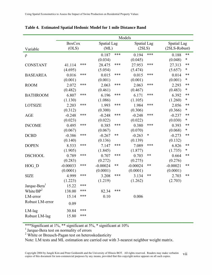
estimated results are reported in Table 3 4 and 5 for the three distance bands between 075
mile 1 mile and 125 mile10
There was a strong presence of spatial lag dependence The robust LM test was highly
significant for spatial lag dependence (p lt 000) whereas it was not for spatial error
dependence The Robust LM test accounts for the presence of misspecification of spatial lag
or spatial error dependence11 The presence of strong lag dependence was consistent across
the 3- to 9-nearest neighbor weights matrix All k 3 5 7 9 weight matrix models were not
significantly different from each other therefore only the diagnostic results and the estimation
of spatial lag model from the 3-nearest neighbor weights matrix are reported12
Two sets of spatial lag models ie the maximum likelihood (ML) and the spatial two-
stage least squares (2SLS) estimation were estimated for the three distance bands The ML
estimation assumes normality In contrast the 2SLS estimation using spatially lagged
Using Spatial Econometrics to Assess the Impact of Swine Production on Residential Property Values
Copyright 2004 by Jungik Kim and Peter Goldsmith and the University of Illinois BOT All rights reserved Readers may make verbatim copies of this document for non-commercial purposes by any means provided that this copyright notice appears on all such copies
13
explanatory variables as instruments is robust to nonnormality and consistent but not
necessarily efficient Given the nonnormality found in the OLS estimates with significant
Jarque-Bera test on normality (p lt 005) the 2SLS estimates seemed more appropriate than the
ML estimation In addition the 2SLS-robust estimation can be an alternative to the ML
estimation when heteroskedasticity is present In fact strong evidence of heteroskedasticity
was present as indicated by significant White test (p lt 005)
All housing physical variables (BASEAREA ROOM BATHROOM LOTSIZE and
AGE) were significant at a 1 significance level and showed the expected signs The
locational variables (INCOME DCBD DOPEN and DSCHOOL) were significant at 5
INCOME was positive meaning that property values are positively associated with
household income The negative DCBD meant that property values declined if they were
located further away from the CBD due to a lack of accessibility The positive DOPEN and
DSCHOOL suggested that the proximity to an open space and a school was not considered as
an amenity in rural areas but instead may be viewed as a lack of accessibility13 The two
variables related to hog impact (HOG_D and SIZE) were significant at 10 with a negative
HOG_D and a positive SIZE The negative HOG_D suggested that hog farms caused
negative effects on property values The positive SIZE implied that house values were higher
if they had large farms in the neighborhood suggesting for scale economies in abatement of
environmental impact of hog farms
Consistent with the results of the robust LM test the spatial autoregressive parameter (ρ) in
the ML estimation was positive and highly significant for all three distance bands (p lt 000)
Compared with the OLS estimates all variables retained their signs and significance but the
magnitude of the coefficients decreased in the ML estimates as the spatial lag effect was then
Using Spatial Econometrics to Assess the Impact of Swine Production on Residential Property Values
Copyright 2004 by Jungik Kim and Peter Goldsmith and the University of Illinois BOT All rights reserved Readers may make verbatim copies of this document for non-commercial purposes by any means provided that this copyright notice appears on all such copies
14
incorporated into the model This suggests that the OLS estimates will be biased if spatial
lag dependence is not accounted for The magnitude of the spatial autoregressive parameter
captured the extent to which a house value at one location was related to its neighbors For
example ρ was about 02 for the 1-mile distance band meaning one-fifth of the house value
could be explained by the values of the neighboring houses After the spatial lag effect was
introduced there was no remaining spatial error dependence as the LM test was no longer
significant for error dependence As in the OLS estimation however heteroskedasticity was
still present in the ML estimation Subsequently the 2SLS and 2SLS-robust estimations
were carried out to address nonnormality and heteroskedasticity Compared with the ML
estimates the change in the coefficients was more pronounced in the 2SLS-robust estimation
than in the 2SLS estimation given that the 2SLS-robust estimation took heteroskedasticity
into account All variables retained their signs and significance in the 2SLS and 2SLS-robust
estimations14
Accounting for spatial autocorrelation in housing prices significantly changed the
magnitude of the impact of hog farms on property values In the OLS estimates property
values declined per hog by -$051 at 075 mile -$068 at 1 mile and -$053 at 125 mile
When spatial autocorrelation was taken into account in the form of spatial lag dependence
the negative impact on property loss was mitigated on average by 18 Specifically in
spatial lag model property value losses decreased 4 cents (8) to -$047 at 075 mile 16
cents (24) to -$052 at 1 mile and 11cents (21) to -$042 at 125 mile Thus the impact
on the value of the median house ($63520) 1 mile from a swine facility with 10000 head
was -$5200 or 8
Using Spatial Econometrics to Assess the Impact of Swine Production on Residential Property Values
Copyright 2004 by Jungik Kim and Peter Goldsmith and the University of Illinois BOT All rights reserved Readers may make verbatim copies of this document for non-commercial purposes by any means provided that this copyright notice appears on all such copies
15
Conclusion
This article examined spatial autocorrelation in housing prices in the assessment of negative
externality of hog farms on surrounding rural property values Spatial autocorrelation in
housing price is inherent in hedonic models using locational variables such as median
household income by census block-group or distance to the facility under study Substantial
spatial autocorrelation was found in OLS estimates A spatial lag dependence model was
developed to correct for spatial autocorrelation as well as nonnormality and
heteroskedasticity The results from the 2SLS-robust estimation showed that when spatial
autocorrelation was explicitly accounted for the negative impact of hog farms on property
loss was mitigated on average by 18
The findings of this article provide prescription for future hedonic studies in rural settings
The conventional use of sale prices as the dependent variable may overlook spatial
autocorrelation in rural property values because they do not represent all rural properties
Turnover is low in rural areas and some rural houses may have never been sold Predicting
missing sale prices can be an alternative using a geostatistical approach (see Dubin) It
remains to be seen how realistic such prediction can be if price is made to be a function of
distance Assessed property values were used for this research to remedy this problem
creating a more spatially contiguous dataset
Using Spatial Econometrics to Assess the Impact of Swine Production on Residential Property Values
Copyright 2004 by Jungik Kim and Peter Goldsmith and the University of Illinois BOT All rights reserved Readers may make verbatim copies of this document for non-commercial purposes by any means provided that this copyright notice appears on all such copies
16
Endnotes 1 There are nine existing studies on the impact of swine operations on property values See Kim Goldsmith and Thomas for an overview 2 The covariogram for the distribution of residuals is defined as )()()( jiji ssCovssC ξξ=minus
for all ( is js ) The semicovariogram dividing the covariogram by 2 is more commonly used to describe how spatial dependence changes as the distance between two observations increases Typically the semicovariogram curve is upward sloping leveling off at some distance (the sill) See Cressie for technical details 3 The weights also can be based on economic distance or general metric such as a social network structure See Anselin and Bera and Anselin (2002) for details 4 For the further exposition of a spatial weights matrix see Anselin (1988 2002) 5 There are 12 and 317 urban houses within 1 mile and 15 mile distance of the nearest farm respectively 6 An additional outlier was identified and excluded from the sample See Kim for details 7 Division of Water Resources website ldquoImportant Facts about Lists of Animal Operationsrdquo ftph2oenrstatencuspubNon-DischargeAnimal20Operations20Info 8 Environmental Defense website httpwwwscorecardorgenv-releasesdefaw_wasteshtml 9 see Kim Goldsmith and Thomas for a complete discussion of the Box-Cox hedonic Swine Impact Model 10 Results for closer and further distance bands (05 mile and beyond 175 mile up to 3 mile) are not reported as the variable of interest HOG_D was not significant The people who were living in close proximity within a 05-mile distance could be related to the hog farms and may be more tolerant of them thereby having no negative effect on assessed values HOG_D was also not significant for the distance band beyond 175 mile up to 3 mile For two distance bands (15 and 175 mile) the results of the robust LM test indicated that both spatial lag and error dependence were present preventing the estimation of the spatial lag or spatial error dependence model 11 In practice the LM test statistic can be significant for both spatial lag and spatial error dependence but the robust LM test statistics point to spatial lag or spatial error dependence 12 The number of nearest neighbors selected as a weights matrix in real estate studies ranges from 3 (Can and Megbolugbe) up to 15 nearest neighbors (Pace et al) The use of 3-nearest neighbor weights matrix for this article conforms to the practice of using three sales comparables in real estate appraisal (Lusht) 13 The expected sign for DOPEN was either positive or negative It could be negative if people valued living near an open space in a more quiet environment or it could be positive if living near open space was viewed as a lack of accessibility The expected sign for DSCHOOL was negative as distance was negatively associated with the degree of accessibility to the school 14 The only exception was HOG _D in the 2SLS-robust estimation for the 075-mile distance band But given that HOG_D was only marginally insignificant (p = 012) in the case of the 075-mile distance band the 2SLS-robust estimation would be the basis for estimating the marginal price in the spatial hedonic model
Using Spatial Econometrics to Assess the Impact of Swine Production on Residential Property Values
Copyright 2004 by Jungik Kim and Peter Goldsmith and the University of Illinois BOT All rights reserved Readers may make verbatim copies of this document for non-commercial purposes by any means provided that this copyright notice appears on all such copies
i
References Anselin L Spatial Econometrics Methods and Models Dordrecht Kluwer Academic 1988 _________ ldquoSpatial Econometricsrdquo Companion to Theoretical Econometrics Badi Baltagi ed pp 310-
330 Oxford Basil Blackwell 2001a _________ ldquoRaorsquos Score Test in Spatial Econometricsrdquo Journal of Statistical Planning and Inference 97
(2001b) 113-139 _________ ldquoUnder the Hood Issues in the Specification and Interpretation of Spatial Regression
Modelsrdquo Agricultural Economics 27 (2002) 247-267 Anselin L and A K Bera ldquoSpatial Dependence in Linear Regression Models with an Introduction to
Spatial Econometricsrdquo Handbook of Applied Economic Statistics A Ullah and D E A Giles eds pp 237-289 New York Marcel Dekker 1998
Basu S and T G Thibodeau ldquoAnalysis of Spatial Autocorrelation in House Pricesrdquo Journal of Real Estate and Economics 17 (1998) 61-85
Beron K J Y Hanson J Murdoch and M Thayer ldquoHedonic Price Functions and Spatial Dependence Implications for the Demand for Urban Air Qualityrdquo Advances in Spatial Econometrics L Anselin R Florax and S Rey eds Heidelberg Springer-Verlag (in press)
Can A ldquoThe Measurement of Neighborhood Dynamics in Urban House Pricesrdquo Economic Geography 66 (1990)203-222
Can A and I Megbolugbe ldquoSpatial Dependence and House Price Index Constructionrdquo Journal of Real Estate Finance and Economics 14 (1997) 203-222
Cressie N A Statistics for Spatial Data New York Wiley 1993 Cropper M L L B Deck and K E McConnell ldquoOn the Choice of Functional Form for Hedonic
Functionrdquo The Review of Economics and Statistics 70 (1988) 668 - 675 Davidson R and J G MacKinnon Estimation and inference in Econometrics Oxford Oxford
University Press 1993 Dubin R A ldquoPredicting House Prices Using Multiple Listings Datardquo Journal of Real Estate Finance
and Economics 17 (1998) 35-59 Dubin R R K Pace and T G Thibodeau ldquoSpatial Autoregression Techniques for Real Estate Datardquo
Journal of Real Estate Literature 7 (1999) 79-95 Hite D W Chern F Hitzhusen and A Randall ldquoProperty-value Impacts of an Environmental
Disamenity The case of landfillsrdquo Journal of Real Estate Finance and Economics 22 (2001)185-202 Kiel K and J Zabel ldquoEstimating the Economic Benefits of Cleaning Up Superfund Sites The Case of
Woburn Massachusettsrdquo Journal of Real Estate Finance and Economics 22 (2001) 163-184 Kim J ldquoAn Assessment of the Discommodity Effects of Swine Production on Rural Property Values
Spatial Analysisrdquo PhD dissertation University of Illinois at Urbana-Champaign 2004 Kim J P Goldsmith and M Thomas ldquoAn Assessment of the Discommodity Effects of Swine
Production on Rural Property Values Review of Agricultural Economics Submitted June 2004 Kim C W T T Phipps and L Anselin ldquoMeasuring the Benefits of Air Quality Improvement A
Spatial Hedonic Approachrdquo Journal of Environmental Economics and Management 45 (2003) 24-39 Kohlhase J E ldquoThe Impact of Toxic Waste Sites on Housing Valuerdquo Journal of Urban Economics 30
(1991)1-26 Lusht K M Real Estate Valuation Principles and Applications New York McGraw-Hill 2000 Pace R K and O W Gilley ldquoUsing the Spatial Configuration of the Data to Improve Estimationrdquo
Journal of Real Estate Finance and Economics 14 (1997) 333-340 Pace R K R Barry J M Clapp and M Rodriquez ldquoSpatiotemporal Autoregressive Models of
Neighborhood Effectsrdquo Journal of Real Estate Finance and Economics 17 (1988)5-13
Using Spatial Econometrics to Assess the Impact of Swine Production on Residential Property Values
Copyright 2004 by Jungik Kim and Peter Goldsmith and the University of Illinois BOT All rights reserved Readers may make verbatim copies of this document for non-commercial purposes by any means provided that this copyright notice appears on all such copies
ii
Appendix The derivation of the marginal price of the spatial hedonic model follows Kim Phipps and Anselin
(pp 34-35) First define the spatial lag model with Box-Cox transformed as
(1) εβρ λλ ++= XWYY )()(
where )(λY is a )1( timesn column vector of transformed assessed values W is a )( nntimes weights matrix X
is a )( kntimes matrix (where k is the number of explanatory variables) β is a )1( timesk column vector and
Let ερν 1][ minusminus= WI and 1][ minusminus= WIA ρ then
(3) νβλ += XAY )(
Equation (3) can be written as
(4)
⎥⎥⎥⎥⎥⎥
⎦
⎤
⎢⎢⎢⎢⎢⎢
⎣
⎡
+
⎥⎥⎥⎥⎥⎥
⎦
⎤
⎢⎢⎢⎢⎢⎢
⎣
⎡
sdot
⎥⎥⎥⎥⎥⎥
⎦
⎤
⎢⎢⎢⎢⎢⎢
⎣
⎡
sdot
⎥⎥⎥⎥⎥⎥
⎦
⎤
⎢⎢⎢⎢⎢⎢
⎣
⎡
=
⎥⎥⎥⎥⎥⎥⎥
⎦
⎤
⎢⎢⎢⎢⎢⎢⎢
⎣
⎡
nknnn
n
n
nnn
n
n
n xx
xxxxxx
aa
aaaaaa
Y
Y
Y
ν
νν
β
ββ
λ
λ
λ
2
1
2
1
1
22221
11211
1
22221
11211
)(
)(2
)(1
Define kX as a column vector )1( timesn of one housing characteristic The marginal price can then be
derived by taking the derivative of both sides of Equation (4) First the derivative of )1()( timesnY λ
with respect to kX is defined as follows
(5)
⎥⎥⎥⎥⎥⎥⎥
⎦
⎤
⎢⎢⎢⎢⎢⎢⎢
⎣
⎡
partpartpartpartpartpart
partpartpartpartpartpart
partpartpartpartpartpart
=partpart
nknknkn
nkkk
nkkk
k
xYxYxY
xYxYxY
xYxYxY
XY
)(2
)(1
)(
)(22
)(21
)(2
)(12
)(11
)(1
)(
λλλ
λλλ
λλλ
λ
Using Spatial Econometrics to Assess the Impact of Swine Production on Residential Property Values
Copyright 2004 by Jungik Kim and Peter Goldsmith and the University of Illinois BOT All rights reserved Readers may make verbatim copies of this document for non-commercial purposes by any means provided that this copyright notice appears on all such copies
iii
)1(
21
22212
12111
)1(
kk
nknknkn
nkkk
nkkk
k XYY
xYxYxY
xYxYxYxYxYxY
Ypartpart
=
⎥⎥⎥⎥⎥⎥
⎦
⎤
⎢⎢⎢⎢⎢⎢
⎣
⎡
partpartpartpartpartpart
partpartpartpartpartpartpartpartpartpartpartpart
= minusminus λλ
On the other hand the derivative on the right side of Equation (4) with respect to kX is
(6) 1
21
22221
11211
][
minusminus==
⎥⎥⎥⎥⎥⎥
⎦
⎤
⎢⎢⎢⎢⎢⎢
⎣
⎡
WIA
aaa
aaaaaa
kk
nnknknk
nkkk
nkkk
ρββ
βββ
ββββββ
It follows that
(7) )1(1
][ minusminusminus=
partpart
λ
βρk
k
k YWI
XY
The marginal price of the spatial lag hedonic model consists of two elements The first element
1][ minusminus WI ρ amounts to a spatial multiplier and can be expanded into an infinite series
(12) ][ 221 +++=minus minus WWIWI ρρρ
)1
1(ρminus
= if W is row-standardized and 1|| ltρ
The presence of a spatial multiplier accounts for spatial spillover effects where a change in the
property value at one location affects all other locations whereas the degree of spillover gradually
diminishes over space In the case of hog farms the spatial multiplier captures the spillover effects
of an environmental impact caused by hog farms over k-nearest neighbors The second term )1( minusλ
β
k
k
Y
is due to Box-Cox transformation and reflects nonlinear relationship between property values and
housing attributes
Using Spatial Econometrics to Assess the Impact of Swine Production on Residential Property Values
Copyright 2004 by Jungik Kim and Peter Goldsmith and the University of Illinois BOT All rights reserved Readers may make verbatim copies of this document for non-commercial purposes by any means provided that this copyright notice appears on all such copies
iv
1
2 3 4
5
Figure 1 Neighbors in Regular Grid
Table 1 Spatial Weights Matrix
0 0 1 0 0 0 0 1 0 0
0 0 1 0 0 0 0 1 0 0
1 1 0 1 1 025 025 0 025 025
0 0 1 0 0 0 0 1 0 0
0 0 1 0 0 0 0 1 0 0
Using Spatial Econometrics to Assess the Impact of Swine Production on Residential Property Values
Copyright 2004 by Jungik Kim and Peter Goldsmith and the University of Illinois BOT All rights reserved Readers may make verbatim copies of this document for non-commercial purposes by any means provided that this copyright notice appears on all such copies
v
Table 2 Descriptive Statistics for Houses within 3 mile Distance (n = 2155) Variables Definition Mean Std
Dev Min Max
Dependent Variable
VALUE Assessed property values ($) 81862 60892 6260 628710
Independent variable
BASEAREA Base area (sq ft) 1461 449 480 3876
ROOM Number of rooms 58 11 2 13
BATHROOM Number of bathrooms 16 06 1 6
LOTSIZE Lot size (acres) 14 16 005 10
AGE Age of house (yrs) 32 25 1 173
INCOME Median household income by census
block-group ($1000)
362 113 221 614
DCDB Distance to the central business
district (miles)
141 63 29 267
DSCHOOL Distance to the nearest school (miles) 38 21 01 92
DOPEN Distance to the nearest open space
(miles)
02 02 0001 13
HOG_D Number of hogs divided by distance
to the nearest farm
3158 3779 264 32555
SIZE 1 if a farm is large (gt 2500 head) 05 05 0 1
Using Spatial Econometrics to Assess the Impact of Swine Production on Residential Property Values
Copyright 2004 by Jungik Kim and Peter Goldsmith and the University of Illinois BOT All rights reserved Readers may make verbatim copies of this document for non-commercial purposes by any means provided that this copyright notice appears on all such copies
vi
Table 3 Estimated Spatial Hedonic Model for 075 Mile Distance Band
Significant at 1 significant at 5 significant at 10 1 Jarque-Bera test on normality of errors 2 White or Breusch-Pagan test on heteroskedasticity Note LM tests and ML estimation are carried out with 3-nearest neighbor weight matrix
Using Spatial Econometrics to Assess the Impact of Swine Production on Residential Property Values
Copyright 2004 by Jungik Kim and Peter Goldsmith and the University of Illinois BOT All rights reserved Readers may make verbatim copies of this document for non-commercial purposes by any means provided that this copyright notice appears on all such copies
vii
Table 4 Estimated Spatial Hedonic Model for 1 mile Distance Band
Significant at 1 significant at 5 significant at 10 1 Jarque-Bera test on normality of errors 2 White or Breusch-Pagan test on heteroskedasticity Note LM tests and ML estimation are carried out with 3-nearest neighbor weight matrix
Using Spatial Econometrics to Assess the Impact of Swine Production on Residential Property Values
Copyright 2004 by Jungik Kim and Peter Goldsmith and the University of Illinois BOT All rights reserved Readers may make verbatim copies of this document for non-commercial purposes by any means provided that this copyright notice appears on all such copies
viii
Table 5 Estimated Spatial Hedonic Model for 125 Mile Distance Band
Significant at 1 significant at 5 significant at 10 1 Jarque-Bera test on normality of errors 2 White or Breusch-Pagan test on heteroskedasticity Note LM tests and ML estimation are carried out with 3-nearest neighbor weight matrix Figure 1
Using Spatial Econometrics to Assess the Impact of Swine Production on Residential Property Values
Copyright 2004 by Jungik Kim and Peter Goldsmith and the University of Illinois BOT All rights reserved Readers may make verbatim copies of this document for non-commercial purposes by any means provided that this copyright notice appears on all such copies
1
Abstract A spatial hedonic model is developed to assess monetary harm of confined animal feeding
operations (CAFOs) on property values taking explicitly spatial dependence in property
values into account Spatial autocorrelation was found in the form of spatial lag dependence
not spatial error dependence When spatial lag dependence is explicitly taken into account on
average the impact is reduced by 18 The magnitude of the spatial autoregressive
parameter was about 02 for the 1-mile distance band meaning one-fifth of the house value
could be explained by the values of the neighboring houses
Key Words Spatial hedonics spatial autocorrelation spatial lag dependence spatial error
Using Spatial Econometrics to Assess the Impact of Swine Production on Residential Property Values
Copyright 2004 by Jungik Kim and Peter Goldsmith and the University of Illinois BOT All rights reserved Readers may make verbatim copies of this document for non-commercial purposes by any means provided that this copyright notice appears on all such copies
2
Introduction Hedonic models in housing and real estate have traditionally used housing physical attributes
and locational characteristics variables to estimate how a certain housing attribute marginally
contributes to housing price Examples of physical attributes variable include floor area the
number of rooms the number of bathrooms or house age For locational characteristics two
kinds of measures are commonly employed an accessibility measure such as distance to the
Central Business District (CBD) and a neighborhood indicator measure such as median
household income Housing values for example would be negatively associated with
distance to CBD due to increased transportation cost Similarly median household income
can be an indicator for neighborhood quality Hedonic models are also used to measure the
negative externality of a noxious facility such as a landfill or a hazardous waste site (see
Kohlhase Kiel and Zabel and Hite et al among others) Distance to such a facility is
additionally used as a locational variable to examine how the negative impacts of the facility
are a function of distance
Hedonic models using locational variables however do not fully account for spatial
autocorrelation in housing prices Spatial autocorrelation refers to the cluster of similar
values in space (Anselin and Bera) Housing prices are spatially autocorrelated because
neighborhood residential properties share location amenities such as public services (Dubin
Basu and Thibodeau) The boundaries of neighborhoods are not always clear-cut and the
objective measures of neighborhood quality are often difficult to obtain The residuals from
hedonic models are likely to be spatially autocorrelated OLS estimates then will be unbiased
but inefficient (Dubin Pace and Thibodeau) Spatial autocorrelation also arises from a
mismatch in spatial scale (Anselin and Bera) Two situations can be discerned First using
an indicator variable for neighborhood quality such as median income will induce a spatial
Using Spatial Econometrics to Assess the Impact of Swine Production on Residential Property Values
Copyright 2004 by Jungik Kim and Peter Goldsmith and the University of Illinois BOT All rights reserved Readers may make verbatim copies of this document for non-commercial purposes by any means provided that this copyright notice appears on all such copies
3
mismatch as the data is only available on the census tract or block-group level The spatial
scale of the census tract or block-group level is larger than that of an individual house
resulting in positive spatial autocorrelation Similarly in the case of a noxious facility and its
surrounding properties the negative impacts of the facility tend to spill across houses The
spatial scale of the impact is larger than an individual house and causes spatial
autocorrelation In the presence of spatial autocorrelation there is a loss of independent
observations The inclusion of a spatially lagged variable in the hedonic model addresses this
loss of information (Anselin and Bera)
The issue of spatial autocorrelation has received little attention in hedonic studies in rural
settings The purpose of this article is to advance the methodology of rural hedonic studies
by developing a spatial hedonic model that explicitly accounts for spatial autocorrelation in
housing prices in the assessment of the monetary harm of confined animal feeding
operations (CAFOs) on rural property values To date none of the existing studies on the
impact of swine operations on property values has addressed the issue of spatial
autocorrelation in housing prices1 This article will contribute to the literature by providing a
benchmark for future hedonic studies of rural land use
Literature Review
Spatial autocorrelation between spatial objects can be formally defined by the moment
condition as follows (Anselin and Bera p 241)
(1) 0][][][]cov[ nesdotminus= jijiji yEyEyyEyy for ji ne
where i j refer to individual locations and iy and jy denote the value of a random variable
at that location The covariance structure becomes spatial when nonzero i j pairs are
Using Spatial Econometrics to Assess the Impact of Swine Production on Residential Property Values
Copyright 2004 by Jungik Kim and Peter Goldsmith and the University of Illinois BOT All rights reserved Readers may make verbatim copies of this document for non-commercial purposes by any means provided that this copyright notice appears on all such copies
4
interpreted ldquoin terms of spatial structure spatial interaction or the spatial arrangement of the
observationsrdquo (Anselin 2001a p 312)
Two approaches direct and indirect representation are suggested in the literature to
model the covariance structure (Anselin 2001a) Direct representation adopted from a
geostatistical approach assumes a continuous surface and expresses spatial interaction as a
continuous function of distance In contrast an indirect representation or lattice approach
presumes that the spatial effect is a function of the interaction among discrete spatial objects
Although direct representation has been applied to real estate markets an indirect approach is
more suited to economic studies dealings with discrete objects in space such as counties or
regions (Anselin and Bera) Moreover specifications used in direct representation have
estimation and identification problems For example the nuisance parameter is not identified
under the null hypothesis resulting in a singular information matrix (Anselin 2001b)
Direct representation focuses on improving spatially autocorrelated residuals by directly
estimating the covariance structure (Dubin Basu and Thibodeau) Spatial covariance is
expressed as a smooth decay function of the distance between observations For example
Dubin specified the covariance structure as
(2) )exp( 21 bdbK ijij minus=
where ijd is the distance between the i and j th observations and 1b and 2b are parameters
to be estimated Basu and Thibodeau used a semivariogram to estimate the covariance
Using Spatial Econometrics to Assess the Impact of Swine Production on Residential Property Values
Copyright 2004 by Jungik Kim and Peter Goldsmith and the University of Illinois BOT All rights reserved Readers may make verbatim copies of this document for non-commercial purposes by any means provided that this copyright notice appears on all such copies
5
where is denotes location of an observation i and )( isξ denotes the hedonic residual for an
observation at is 2
In indirect representation the specification of a spatial process indirectly determines a
covariance structure which requires constructing a relevant spatial weights matrix In
indirect representation two types of spatial dependence spatial lag dependence and error
dependence are conventionally distinguished (Anselin 1988) Spatial lag dependence arises
from spatial interaction between economic agents such as counties or states or mismatch in
spatial scale Spatial lag dependence is modeled by incorporating a spatially lagged
dependent variable in hedonic models analogous to the inclusion of a serially autoregressive
term for the dependent variable ( 1minusty ) in a time-series context The inclusion of a spatial
lagged dependent variable has two implications (Anselin and Bera) First OLS estimates
will be biased and inconsistent because a spatially lagged dependent variable is endogenous
and always correlated with the error term Second the simultaneity must be explicitly
accounted for either in a maximum likelihood estimation framework or by using a proper set
of instrumental variables
On the other hand spatial error dependence arises from noise in the model and can be
specified as a spatial process for the disturbance term The effect of a spatial residual
autocorrelation on the OLS estimator is analogous to time-series results The OLS estimates
will be unbiased but inefficient More efficient estimators are obtained by specifying the
error covariance implied by the spatial process
Spatial Weights Matrix
The specification of a covariance structure in indirect representation requires constructing a
relevant spatial weights matrix The choice of spatial weights is made empirically in many
Using Spatial Econometrics to Assess the Impact of Swine Production on Residential Property Values
Copyright 2004 by Jungik Kim and Peter Goldsmith and the University of Illinois BOT All rights reserved Readers may make verbatim copies of this document for non-commercial purposes by any means provided that this copyright notice appears on all such copies
6
applications as there is very little theoretical guidance in the choice of spatial weights
(Anselin 2002)
A spatial weights matrix usually denoted by W specifies neighborhood sets for each
observation as nonzero elements In each row i a nonzero element ijw defines j as being a
neighbor of i So 1=ijw when i and j are neighbors and 0=ijw otherwise Establishing
the neighborhood set in this fashion reflects the range of spatial interaction In the case of the
housing market for example nonzero pairs in a spatial weights matrix would indicate the
extent of the externality effect on neighboring houses By convention an observation is not a
neighbor to itself so that the diagonal elements are zero ( 0=iiw ) In most cases the spatial
weights matrix is row standardized so that weights across rows are summed to one which
amounts to averaging of the neighboring values and allowing for spatial smoothing
Standardizing weights also makes the spatial parameters comparable between models
There are different ways to define neighborhoods and a weights matrix3 Conventionally
neighbors refer to locations adjacent to each other sharing common boundaries or vertexes
so for example a county in a regular grid will have four neighbors (rook or bishop criterion)
or eight neighbors (queen criterion) (Anselin 2002) For example in Figure 1 the five
observations in a regular grid have one or four neighbors that share borders (rook criterion)
The left side of Table 1 is a corresponding 5 times 5 spatial weights matrix and the right side
shows a standardized weights matrix4
For an irregular grid the number of neighbors will depend on the shape of the grid This
notion of neighbors based on contiguity cannot be applied to rural housing markets because
houses are not contiguous and can be separated by great distances Constructing a weights
Using Spatial Econometrics to Assess the Impact of Swine Production on Residential Property Values
Copyright 2004 by Jungik Kim and Peter Goldsmith and the University of Illinois BOT All rights reserved Readers may make verbatim copies of this document for non-commercial purposes by any means provided that this copyright notice appears on all such copies
7
matrix in rural areas based on contiguity will yield many ldquoislandsrdquo or observations with no
connections and make the analysis of spatial autocorrelation irrelevant
Neighbors can also be defined as the locations within a given distance For the type of
distance a physical distance-band is commonly used (Can Can and Megbolugbe Pace and
Gilley Kim Phipps and Anselin) The number of neighbors however will vary if the sizes
of spatial units differ A distance-band weights matrix is not feasible for rural studies since
lot sizes vary greatly in rural areas Building a weights matrix on a distance band will
produce an uneven number of neighbors from rural clusters (hamlets) or a small number of
neighbors for larger lots (farms)
Alternatively k-nearest neighbors for each house can be employed to address
unconnected houses in a contiguity base or an uneven number of neighbors in a distance-
band case (Can and Megbolugbe Pace et al) Choosing k-nearest neighbors ensures a
constant number of neighbors for each house The idea of k-nearest neighbors corresponds to
the practice of the ldquocomparable-salesrdquo approach employed in residential real estate appraisal
(Can and Megbolugbe)
Empirical Studies
Several hedonic studies in real estate and housing markets have applied an indirect
representation of the covariance structure among spatial objects when addressing spatial
autocorrelation Yet no study examines the issue of spatial autocorrelation in housing prices
in rural settings much less where CAFOs are concerned
Incorporating a spatially lagged dependent variable and spatial parametric drift to
housing prices in Columbus Ohio offered better explanation of the variations than
traditional hedonic price models (Can) Similarly incorporating a spatially lagged dependent
Using Spatial Econometrics to Assess the Impact of Swine Production on Residential Property Values
Copyright 2004 by Jungik Kim and Peter Goldsmith and the University of Illinois BOT All rights reserved Readers may make verbatim copies of this document for non-commercial purposes by any means provided that this copyright notice appears on all such copies
8
variable to consider the house price index in Miami Florida not only increased the
explanatory power of the model reflected in a higher R2 but also addressed to some extent
the problem of omitted housing structure variables (Can and Megbolugbe)
In contrast to these studies specifying a spatially lagged dependent variable a spatially
autocorrelated error term was specified through a weighted average of the errors on nearby
properties for housing data in Boston (Pace and Gilley) The weight was given to each
census tract and set as the distance between two tracts relative to all other tracts The
estimation results showed that modeling spatial dependence of the errors was significantly
beneficial resulting in a 44 reduction of the errors relative to the OLS
A lattice perspective has also been used in the environmental economics literature The
OLS overestimated the effect of air quality on housing prices in Seoul Korea in the presence
of spatial lag dependence (Kim Phipps and Anselin) On the other hand a spatial
autoregressive (SAR) error model did not change the empirical results much in estimating the
demand for air quality in the South Coast Air Basin counties (Beron et al)
Study Area and Data
Craven County located in southeastern North Carolina is chosen as a study area for three
reasons first geographically coded real estate (N = 25684 housing values) and swine
industry data (N = 26 farms and 85000 pigs) are available second the farms are located in
one of the most significant swine regions nationally with the farm size ranging from 600 to
12600 hogs and third land use is heterogeneous where neither agriculture nor non-
agriculture rural residents dominate
Using Spatial Econometrics to Assess the Impact of Swine Production on Residential Property Values
Copyright 2004 by Jungik Kim and Peter Goldsmith and the University of Illinois BOT All rights reserved Readers may make verbatim copies of this document for non-commercial purposes by any means provided that this copyright notice appears on all such copies
9
Three phases of data collection are involved in this study These data include (1)
assessed property values including location and description information (2) general
neighborhood indicators and (3) hog operation and location
Data on assessed property values are available from the Craven County GIS Website
Craven County completed a countywide revaluation of 50000 individual parcels as of
January 1 2002 based on a 8 year total revaluation cycle mandated by North Carolina
General Statutes The County updated new values for all properties in January 2003
For the purpose of analysis rural houses are identified from the Craven parcels map with
the following procedures first since the Craven parcels map includes every parcel including
residential commercial agricultural and open space only parcels whose building type and
land use are residential are deemed to be residential parcels with houses Second only
houses with at least one bedroom and bathroom including mobile homes are selected Third
houses in urban areas (n = 12799) are excluded as they because of their higher population
density may swamp the data compared to the sparsely populated rural areas As a result
1100 urban houses (9) were lost within 2 mile of the nearest farm5 Additionally 91 rural
houses that are located in the same blocks with urban houses were deemed to be urban and
excluded from the sample (Kim) Houses in the two townships (Township 5 and 6) with no
hog farms are also excluded from the sample as the minimum distance from the two
townships to the nearest farm is about 725 and 19 miles respectively Houses with lot size
over 10 acres are considered outliers and excluded to avoid houses with farm or timber tracts
following Palmquist Roka and Vukina6
Information on the general neighborhood indicators is available from the 2000 Census
The Census Bureau reports the median household income and average commuting time to
Using Spatial Econometrics to Assess the Impact of Swine Production on Residential Property Values
Copyright 2004 by Jungik Kim and Peter Goldsmith and the University of Illinois BOT All rights reserved Readers may make verbatim copies of this document for non-commercial purposes by any means provided that this copyright notice appears on all such copies
10
work by the census block-group level The spatial information on the census block-groups is
available in the form of the Census 2000 TIGER (Topologically Integrated Geographic
Encoding and Referencing System) Shapefiles
Data on the 26 hog operations are acquired from the North Carolina Department of
Environment and Natural Resources Division of Water Resources and Craven County
Appraisal Office North Carolina hog data include farm number farm name design capacity
steady-state live weight owners name and mailing address The steady-state live weight
represents the collective weight of all animals at a facility and is a more accurate means of
size comparisons7 The steady-state live weight is divided by an average hog weight (135
lb) to get an average number of animal ldquounitsrdquo for an operation Alternatively the actual
number of hogs could be used to compare farm sizes But data on the number of hogs by
different types such as sows nurseries or piglets are not available Using steady-state live
weight can account for different types of hogs on a farm and is considered as more
representative of the hogs than the actual number of hogs8 The locations of the farms are
identified by comparing ownersrsquo names and parcel IDs from Craven County Appraisal
Officersquos records
Model Specification
The estimation of spatial hedonic model is preceded by diagnostics of spatial autocorrelation
in the hedonic OLS model9 To that end the Lagrange multiplier (LM) tests for spatial lag
dependence and spatial error dependence are used (Anselin 1988) The result of the LM test
determines spatial lag or spatial error dependence Spatial lag dependence is modeled by
Using Spatial Econometrics to Assess the Impact of Swine Production on Residential Property Values
Copyright 2004 by Jungik Kim and Peter Goldsmith and the University of Illinois BOT All rights reserved Readers may make verbatim copies of this document for non-commercial purposes by any means provided that this copyright notice appears on all such copies
11
incorporating a spatially lagged dependent variable (Wy) into the model Specifically spatial
lag model is specified as
(4) εβρ ++sdot= XYWY where ρ is the spatial autoregressive parameter W is the k-nearest neighbor weights matrix
X is a vector of independent variables as above and ε is an error term
Alternatively a spatial error model can be specified with respect to the disturbance term
The most common specification is a spatial autoregressive (SAR) process in the error terms
(5) εβ += XY (6) ξελε += W where ε is an error term λ is the spatial autoregressive coefficient for the error lag εW and
ξ is an uncorrelated and homoskedastic error term
Specific to our context spatial lag dependence model is specified as
+ β4 LOTSIZE + β5 AGE + β6 INCOME + β7 DCBD + β8 DOPEN
+ β9 DSCHOOL + β10 HOG_D + β11 SIZE
where VTF is Box-Cox transformed assessed property values ρ is the spatial autoregressive
parameter W is the k-nearest neighbor weights matrix BASEAREA is the base area of a
house ROOM is the number of rooms BATHROOM is the number of bathrooms LOTSIZE
is lot size AGE is house age INCOME is median household income by census block groups
DCBD is the distance to CBD DOPEN is the distance to nearest open space DSCHOOL is
the distance to the nearest school HOG_D is the number of hogs in the nearest farm divided
by the distance and SIZE is a dummy variable for farm size (= 1 if greater than 2500 head)
Using Spatial Econometrics to Assess the Impact of Swine Production on Residential Property Values
Copyright 2004 by Jungik Kim and Peter Goldsmith and the University of Illinois BOT All rights reserved Readers may make verbatim copies of this document for non-commercial purposes by any means provided that this copyright notice appears on all such copies
12
On the other hand if the LM test points to spatial error dependence the spatial
+ β5 AGE + β6 INCOME + β7 DCBD + β8 DOPEN + β9 DSCHOOL
+ β10 HOG_D + β11 SIZE
where all notations remain the same as in spatial lag dependence model The SAR error model
achieves more efficient estimates by specifying the error covariance (Equation 6)
Estimation Results
The spatial lag model was estimated by taking all houses within certain distance from the
nearest farm starting from 05 mile up to 3 mile with a quarter mile increment The
estimated results are reported in Table 3 4 and 5 for the three distance bands between 075
mile 1 mile and 125 mile10
There was a strong presence of spatial lag dependence The robust LM test was highly
significant for spatial lag dependence (p lt 000) whereas it was not for spatial error
dependence The Robust LM test accounts for the presence of misspecification of spatial lag
or spatial error dependence11 The presence of strong lag dependence was consistent across
the 3- to 9-nearest neighbor weights matrix All k 3 5 7 9 weight matrix models were not
significantly different from each other therefore only the diagnostic results and the estimation
of spatial lag model from the 3-nearest neighbor weights matrix are reported12
Two sets of spatial lag models ie the maximum likelihood (ML) and the spatial two-
stage least squares (2SLS) estimation were estimated for the three distance bands The ML
estimation assumes normality In contrast the 2SLS estimation using spatially lagged
Using Spatial Econometrics to Assess the Impact of Swine Production on Residential Property Values
Copyright 2004 by Jungik Kim and Peter Goldsmith and the University of Illinois BOT All rights reserved Readers may make verbatim copies of this document for non-commercial purposes by any means provided that this copyright notice appears on all such copies
13
explanatory variables as instruments is robust to nonnormality and consistent but not
necessarily efficient Given the nonnormality found in the OLS estimates with significant
Jarque-Bera test on normality (p lt 005) the 2SLS estimates seemed more appropriate than the
ML estimation In addition the 2SLS-robust estimation can be an alternative to the ML
estimation when heteroskedasticity is present In fact strong evidence of heteroskedasticity
was present as indicated by significant White test (p lt 005)
All housing physical variables (BASEAREA ROOM BATHROOM LOTSIZE and
AGE) were significant at a 1 significance level and showed the expected signs The
locational variables (INCOME DCBD DOPEN and DSCHOOL) were significant at 5
INCOME was positive meaning that property values are positively associated with
household income The negative DCBD meant that property values declined if they were
located further away from the CBD due to a lack of accessibility The positive DOPEN and
DSCHOOL suggested that the proximity to an open space and a school was not considered as
an amenity in rural areas but instead may be viewed as a lack of accessibility13 The two
variables related to hog impact (HOG_D and SIZE) were significant at 10 with a negative
HOG_D and a positive SIZE The negative HOG_D suggested that hog farms caused
negative effects on property values The positive SIZE implied that house values were higher
if they had large farms in the neighborhood suggesting for scale economies in abatement of
environmental impact of hog farms
Consistent with the results of the robust LM test the spatial autoregressive parameter (ρ) in
the ML estimation was positive and highly significant for all three distance bands (p lt 000)
Compared with the OLS estimates all variables retained their signs and significance but the
magnitude of the coefficients decreased in the ML estimates as the spatial lag effect was then
Using Spatial Econometrics to Assess the Impact of Swine Production on Residential Property Values
Copyright 2004 by Jungik Kim and Peter Goldsmith and the University of Illinois BOT All rights reserved Readers may make verbatim copies of this document for non-commercial purposes by any means provided that this copyright notice appears on all such copies
14
incorporated into the model This suggests that the OLS estimates will be biased if spatial
lag dependence is not accounted for The magnitude of the spatial autoregressive parameter
captured the extent to which a house value at one location was related to its neighbors For
example ρ was about 02 for the 1-mile distance band meaning one-fifth of the house value
could be explained by the values of the neighboring houses After the spatial lag effect was
introduced there was no remaining spatial error dependence as the LM test was no longer
significant for error dependence As in the OLS estimation however heteroskedasticity was
still present in the ML estimation Subsequently the 2SLS and 2SLS-robust estimations
were carried out to address nonnormality and heteroskedasticity Compared with the ML
estimates the change in the coefficients was more pronounced in the 2SLS-robust estimation
than in the 2SLS estimation given that the 2SLS-robust estimation took heteroskedasticity
into account All variables retained their signs and significance in the 2SLS and 2SLS-robust
estimations14
Accounting for spatial autocorrelation in housing prices significantly changed the
magnitude of the impact of hog farms on property values In the OLS estimates property
values declined per hog by -$051 at 075 mile -$068 at 1 mile and -$053 at 125 mile
When spatial autocorrelation was taken into account in the form of spatial lag dependence
the negative impact on property loss was mitigated on average by 18 Specifically in
spatial lag model property value losses decreased 4 cents (8) to -$047 at 075 mile 16
cents (24) to -$052 at 1 mile and 11cents (21) to -$042 at 125 mile Thus the impact
on the value of the median house ($63520) 1 mile from a swine facility with 10000 head
was -$5200 or 8
Using Spatial Econometrics to Assess the Impact of Swine Production on Residential Property Values
Copyright 2004 by Jungik Kim and Peter Goldsmith and the University of Illinois BOT All rights reserved Readers may make verbatim copies of this document for non-commercial purposes by any means provided that this copyright notice appears on all such copies
15
Conclusion
This article examined spatial autocorrelation in housing prices in the assessment of negative
externality of hog farms on surrounding rural property values Spatial autocorrelation in
housing price is inherent in hedonic models using locational variables such as median
household income by census block-group or distance to the facility under study Substantial
spatial autocorrelation was found in OLS estimates A spatial lag dependence model was
developed to correct for spatial autocorrelation as well as nonnormality and
heteroskedasticity The results from the 2SLS-robust estimation showed that when spatial
autocorrelation was explicitly accounted for the negative impact of hog farms on property
loss was mitigated on average by 18
The findings of this article provide prescription for future hedonic studies in rural settings
The conventional use of sale prices as the dependent variable may overlook spatial
autocorrelation in rural property values because they do not represent all rural properties
Turnover is low in rural areas and some rural houses may have never been sold Predicting
missing sale prices can be an alternative using a geostatistical approach (see Dubin) It
remains to be seen how realistic such prediction can be if price is made to be a function of
distance Assessed property values were used for this research to remedy this problem
creating a more spatially contiguous dataset
Using Spatial Econometrics to Assess the Impact of Swine Production on Residential Property Values
Copyright 2004 by Jungik Kim and Peter Goldsmith and the University of Illinois BOT All rights reserved Readers may make verbatim copies of this document for non-commercial purposes by any means provided that this copyright notice appears on all such copies
16
Endnotes 1 There are nine existing studies on the impact of swine operations on property values See Kim Goldsmith and Thomas for an overview 2 The covariogram for the distribution of residuals is defined as )()()( jiji ssCovssC ξξ=minus
for all ( is js ) The semicovariogram dividing the covariogram by 2 is more commonly used to describe how spatial dependence changes as the distance between two observations increases Typically the semicovariogram curve is upward sloping leveling off at some distance (the sill) See Cressie for technical details 3 The weights also can be based on economic distance or general metric such as a social network structure See Anselin and Bera and Anselin (2002) for details 4 For the further exposition of a spatial weights matrix see Anselin (1988 2002) 5 There are 12 and 317 urban houses within 1 mile and 15 mile distance of the nearest farm respectively 6 An additional outlier was identified and excluded from the sample See Kim for details 7 Division of Water Resources website ldquoImportant Facts about Lists of Animal Operationsrdquo ftph2oenrstatencuspubNon-DischargeAnimal20Operations20Info 8 Environmental Defense website httpwwwscorecardorgenv-releasesdefaw_wasteshtml 9 see Kim Goldsmith and Thomas for a complete discussion of the Box-Cox hedonic Swine Impact Model 10 Results for closer and further distance bands (05 mile and beyond 175 mile up to 3 mile) are not reported as the variable of interest HOG_D was not significant The people who were living in close proximity within a 05-mile distance could be related to the hog farms and may be more tolerant of them thereby having no negative effect on assessed values HOG_D was also not significant for the distance band beyond 175 mile up to 3 mile For two distance bands (15 and 175 mile) the results of the robust LM test indicated that both spatial lag and error dependence were present preventing the estimation of the spatial lag or spatial error dependence model 11 In practice the LM test statistic can be significant for both spatial lag and spatial error dependence but the robust LM test statistics point to spatial lag or spatial error dependence 12 The number of nearest neighbors selected as a weights matrix in real estate studies ranges from 3 (Can and Megbolugbe) up to 15 nearest neighbors (Pace et al) The use of 3-nearest neighbor weights matrix for this article conforms to the practice of using three sales comparables in real estate appraisal (Lusht) 13 The expected sign for DOPEN was either positive or negative It could be negative if people valued living near an open space in a more quiet environment or it could be positive if living near open space was viewed as a lack of accessibility The expected sign for DSCHOOL was negative as distance was negatively associated with the degree of accessibility to the school 14 The only exception was HOG _D in the 2SLS-robust estimation for the 075-mile distance band But given that HOG_D was only marginally insignificant (p = 012) in the case of the 075-mile distance band the 2SLS-robust estimation would be the basis for estimating the marginal price in the spatial hedonic model
Using Spatial Econometrics to Assess the Impact of Swine Production on Residential Property Values
Copyright 2004 by Jungik Kim and Peter Goldsmith and the University of Illinois BOT All rights reserved Readers may make verbatim copies of this document for non-commercial purposes by any means provided that this copyright notice appears on all such copies
i
References Anselin L Spatial Econometrics Methods and Models Dordrecht Kluwer Academic 1988 _________ ldquoSpatial Econometricsrdquo Companion to Theoretical Econometrics Badi Baltagi ed pp 310-
330 Oxford Basil Blackwell 2001a _________ ldquoRaorsquos Score Test in Spatial Econometricsrdquo Journal of Statistical Planning and Inference 97
(2001b) 113-139 _________ ldquoUnder the Hood Issues in the Specification and Interpretation of Spatial Regression
Modelsrdquo Agricultural Economics 27 (2002) 247-267 Anselin L and A K Bera ldquoSpatial Dependence in Linear Regression Models with an Introduction to
Spatial Econometricsrdquo Handbook of Applied Economic Statistics A Ullah and D E A Giles eds pp 237-289 New York Marcel Dekker 1998
Basu S and T G Thibodeau ldquoAnalysis of Spatial Autocorrelation in House Pricesrdquo Journal of Real Estate and Economics 17 (1998) 61-85
Beron K J Y Hanson J Murdoch and M Thayer ldquoHedonic Price Functions and Spatial Dependence Implications for the Demand for Urban Air Qualityrdquo Advances in Spatial Econometrics L Anselin R Florax and S Rey eds Heidelberg Springer-Verlag (in press)
Can A ldquoThe Measurement of Neighborhood Dynamics in Urban House Pricesrdquo Economic Geography 66 (1990)203-222
Can A and I Megbolugbe ldquoSpatial Dependence and House Price Index Constructionrdquo Journal of Real Estate Finance and Economics 14 (1997) 203-222
Cressie N A Statistics for Spatial Data New York Wiley 1993 Cropper M L L B Deck and K E McConnell ldquoOn the Choice of Functional Form for Hedonic
Functionrdquo The Review of Economics and Statistics 70 (1988) 668 - 675 Davidson R and J G MacKinnon Estimation and inference in Econometrics Oxford Oxford
University Press 1993 Dubin R A ldquoPredicting House Prices Using Multiple Listings Datardquo Journal of Real Estate Finance
and Economics 17 (1998) 35-59 Dubin R R K Pace and T G Thibodeau ldquoSpatial Autoregression Techniques for Real Estate Datardquo
Journal of Real Estate Literature 7 (1999) 79-95 Hite D W Chern F Hitzhusen and A Randall ldquoProperty-value Impacts of an Environmental
Disamenity The case of landfillsrdquo Journal of Real Estate Finance and Economics 22 (2001)185-202 Kiel K and J Zabel ldquoEstimating the Economic Benefits of Cleaning Up Superfund Sites The Case of
Woburn Massachusettsrdquo Journal of Real Estate Finance and Economics 22 (2001) 163-184 Kim J ldquoAn Assessment of the Discommodity Effects of Swine Production on Rural Property Values
Spatial Analysisrdquo PhD dissertation University of Illinois at Urbana-Champaign 2004 Kim J P Goldsmith and M Thomas ldquoAn Assessment of the Discommodity Effects of Swine
Production on Rural Property Values Review of Agricultural Economics Submitted June 2004 Kim C W T T Phipps and L Anselin ldquoMeasuring the Benefits of Air Quality Improvement A
Spatial Hedonic Approachrdquo Journal of Environmental Economics and Management 45 (2003) 24-39 Kohlhase J E ldquoThe Impact of Toxic Waste Sites on Housing Valuerdquo Journal of Urban Economics 30
(1991)1-26 Lusht K M Real Estate Valuation Principles and Applications New York McGraw-Hill 2000 Pace R K and O W Gilley ldquoUsing the Spatial Configuration of the Data to Improve Estimationrdquo
Journal of Real Estate Finance and Economics 14 (1997) 333-340 Pace R K R Barry J M Clapp and M Rodriquez ldquoSpatiotemporal Autoregressive Models of
Neighborhood Effectsrdquo Journal of Real Estate Finance and Economics 17 (1988)5-13
Using Spatial Econometrics to Assess the Impact of Swine Production on Residential Property Values
Copyright 2004 by Jungik Kim and Peter Goldsmith and the University of Illinois BOT All rights reserved Readers may make verbatim copies of this document for non-commercial purposes by any means provided that this copyright notice appears on all such copies
ii
Appendix The derivation of the marginal price of the spatial hedonic model follows Kim Phipps and Anselin
(pp 34-35) First define the spatial lag model with Box-Cox transformed as
(1) εβρ λλ ++= XWYY )()(
where )(λY is a )1( timesn column vector of transformed assessed values W is a )( nntimes weights matrix X
is a )( kntimes matrix (where k is the number of explanatory variables) β is a )1( timesk column vector and
Let ερν 1][ minusminus= WI and 1][ minusminus= WIA ρ then
(3) νβλ += XAY )(
Equation (3) can be written as
(4)
⎥⎥⎥⎥⎥⎥
⎦
⎤
⎢⎢⎢⎢⎢⎢
⎣
⎡
+
⎥⎥⎥⎥⎥⎥
⎦
⎤
⎢⎢⎢⎢⎢⎢
⎣
⎡
sdot
⎥⎥⎥⎥⎥⎥
⎦
⎤
⎢⎢⎢⎢⎢⎢
⎣
⎡
sdot
⎥⎥⎥⎥⎥⎥
⎦
⎤
⎢⎢⎢⎢⎢⎢
⎣
⎡
=
⎥⎥⎥⎥⎥⎥⎥
⎦
⎤
⎢⎢⎢⎢⎢⎢⎢
⎣
⎡
nknnn
n
n
nnn
n
n
n xx
xxxxxx
aa
aaaaaa
Y
Y
Y
ν
νν
β
ββ
λ
λ
λ
2
1
2
1
1
22221
11211
1
22221
11211
)(
)(2
)(1
Define kX as a column vector )1( timesn of one housing characteristic The marginal price can then be
derived by taking the derivative of both sides of Equation (4) First the derivative of )1()( timesnY λ
with respect to kX is defined as follows
(5)
⎥⎥⎥⎥⎥⎥⎥
⎦
⎤
⎢⎢⎢⎢⎢⎢⎢
⎣
⎡
partpartpartpartpartpart
partpartpartpartpartpart
partpartpartpartpartpart
=partpart
nknknkn
nkkk
nkkk
k
xYxYxY
xYxYxY
xYxYxY
XY
)(2
)(1
)(
)(22
)(21
)(2
)(12
)(11
)(1
)(
λλλ
λλλ
λλλ
λ
Using Spatial Econometrics to Assess the Impact of Swine Production on Residential Property Values
Copyright 2004 by Jungik Kim and Peter Goldsmith and the University of Illinois BOT All rights reserved Readers may make verbatim copies of this document for non-commercial purposes by any means provided that this copyright notice appears on all such copies
iii
)1(
21
22212
12111
)1(
kk
nknknkn
nkkk
nkkk
k XYY
xYxYxY
xYxYxYxYxYxY
Ypartpart
=
⎥⎥⎥⎥⎥⎥
⎦
⎤
⎢⎢⎢⎢⎢⎢
⎣
⎡
partpartpartpartpartpart
partpartpartpartpartpartpartpartpartpartpartpart
= minusminus λλ
On the other hand the derivative on the right side of Equation (4) with respect to kX is
(6) 1
21
22221
11211
][
minusminus==
⎥⎥⎥⎥⎥⎥
⎦
⎤
⎢⎢⎢⎢⎢⎢
⎣
⎡
WIA
aaa
aaaaaa
kk
nnknknk
nkkk
nkkk
ρββ
βββ
ββββββ
It follows that
(7) )1(1
][ minusminusminus=
partpart
λ
βρk
k
k YWI
XY
The marginal price of the spatial lag hedonic model consists of two elements The first element
1][ minusminus WI ρ amounts to a spatial multiplier and can be expanded into an infinite series
(12) ][ 221 +++=minus minus WWIWI ρρρ
)1
1(ρminus
= if W is row-standardized and 1|| ltρ
The presence of a spatial multiplier accounts for spatial spillover effects where a change in the
property value at one location affects all other locations whereas the degree of spillover gradually
diminishes over space In the case of hog farms the spatial multiplier captures the spillover effects
of an environmental impact caused by hog farms over k-nearest neighbors The second term )1( minusλ
β
k
k
Y
is due to Box-Cox transformation and reflects nonlinear relationship between property values and
housing attributes
Using Spatial Econometrics to Assess the Impact of Swine Production on Residential Property Values
Copyright 2004 by Jungik Kim and Peter Goldsmith and the University of Illinois BOT All rights reserved Readers may make verbatim copies of this document for non-commercial purposes by any means provided that this copyright notice appears on all such copies
iv
1
2 3 4
5
Figure 1 Neighbors in Regular Grid
Table 1 Spatial Weights Matrix
0 0 1 0 0 0 0 1 0 0
0 0 1 0 0 0 0 1 0 0
1 1 0 1 1 025 025 0 025 025
0 0 1 0 0 0 0 1 0 0
0 0 1 0 0 0 0 1 0 0
Using Spatial Econometrics to Assess the Impact of Swine Production on Residential Property Values
Copyright 2004 by Jungik Kim and Peter Goldsmith and the University of Illinois BOT All rights reserved Readers may make verbatim copies of this document for non-commercial purposes by any means provided that this copyright notice appears on all such copies
v
Table 2 Descriptive Statistics for Houses within 3 mile Distance (n = 2155) Variables Definition Mean Std
Dev Min Max
Dependent Variable
VALUE Assessed property values ($) 81862 60892 6260 628710
Independent variable
BASEAREA Base area (sq ft) 1461 449 480 3876
ROOM Number of rooms 58 11 2 13
BATHROOM Number of bathrooms 16 06 1 6
LOTSIZE Lot size (acres) 14 16 005 10
AGE Age of house (yrs) 32 25 1 173
INCOME Median household income by census
block-group ($1000)
362 113 221 614
DCDB Distance to the central business
district (miles)
141 63 29 267
DSCHOOL Distance to the nearest school (miles) 38 21 01 92
DOPEN Distance to the nearest open space
(miles)
02 02 0001 13
HOG_D Number of hogs divided by distance
to the nearest farm
3158 3779 264 32555
SIZE 1 if a farm is large (gt 2500 head) 05 05 0 1
Using Spatial Econometrics to Assess the Impact of Swine Production on Residential Property Values
Copyright 2004 by Jungik Kim and Peter Goldsmith and the University of Illinois BOT All rights reserved Readers may make verbatim copies of this document for non-commercial purposes by any means provided that this copyright notice appears on all such copies
vi
Table 3 Estimated Spatial Hedonic Model for 075 Mile Distance Band
Significant at 1 significant at 5 significant at 10 1 Jarque-Bera test on normality of errors 2 White or Breusch-Pagan test on heteroskedasticity Note LM tests and ML estimation are carried out with 3-nearest neighbor weight matrix
Using Spatial Econometrics to Assess the Impact of Swine Production on Residential Property Values
Copyright 2004 by Jungik Kim and Peter Goldsmith and the University of Illinois BOT All rights reserved Readers may make verbatim copies of this document for non-commercial purposes by any means provided that this copyright notice appears on all such copies
vii
Table 4 Estimated Spatial Hedonic Model for 1 mile Distance Band
Significant at 1 significant at 5 significant at 10 1 Jarque-Bera test on normality of errors 2 White or Breusch-Pagan test on heteroskedasticity Note LM tests and ML estimation are carried out with 3-nearest neighbor weight matrix
Using Spatial Econometrics to Assess the Impact of Swine Production on Residential Property Values
Copyright 2004 by Jungik Kim and Peter Goldsmith and the University of Illinois BOT All rights reserved Readers may make verbatim copies of this document for non-commercial purposes by any means provided that this copyright notice appears on all such copies
viii
Table 5 Estimated Spatial Hedonic Model for 125 Mile Distance Band
Significant at 1 significant at 5 significant at 10 1 Jarque-Bera test on normality of errors 2 White or Breusch-Pagan test on heteroskedasticity Note LM tests and ML estimation are carried out with 3-nearest neighbor weight matrix Figure 1
Using Spatial Econometrics to Assess the Impact of Swine Production on Residential Property Values
Copyright 2004 by Jungik Kim and Peter Goldsmith and the University of Illinois BOT All rights reserved Readers may make verbatim copies of this document for non-commercial purposes by any means provided that this copyright notice appears on all such copies
2
Introduction Hedonic models in housing and real estate have traditionally used housing physical attributes
and locational characteristics variables to estimate how a certain housing attribute marginally
contributes to housing price Examples of physical attributes variable include floor area the
number of rooms the number of bathrooms or house age For locational characteristics two
kinds of measures are commonly employed an accessibility measure such as distance to the
Central Business District (CBD) and a neighborhood indicator measure such as median
household income Housing values for example would be negatively associated with
distance to CBD due to increased transportation cost Similarly median household income
can be an indicator for neighborhood quality Hedonic models are also used to measure the
negative externality of a noxious facility such as a landfill or a hazardous waste site (see
Kohlhase Kiel and Zabel and Hite et al among others) Distance to such a facility is
additionally used as a locational variable to examine how the negative impacts of the facility
are a function of distance
Hedonic models using locational variables however do not fully account for spatial
autocorrelation in housing prices Spatial autocorrelation refers to the cluster of similar
values in space (Anselin and Bera) Housing prices are spatially autocorrelated because
neighborhood residential properties share location amenities such as public services (Dubin
Basu and Thibodeau) The boundaries of neighborhoods are not always clear-cut and the
objective measures of neighborhood quality are often difficult to obtain The residuals from
hedonic models are likely to be spatially autocorrelated OLS estimates then will be unbiased
but inefficient (Dubin Pace and Thibodeau) Spatial autocorrelation also arises from a
mismatch in spatial scale (Anselin and Bera) Two situations can be discerned First using
an indicator variable for neighborhood quality such as median income will induce a spatial
Using Spatial Econometrics to Assess the Impact of Swine Production on Residential Property Values
Copyright 2004 by Jungik Kim and Peter Goldsmith and the University of Illinois BOT All rights reserved Readers may make verbatim copies of this document for non-commercial purposes by any means provided that this copyright notice appears on all such copies
3
mismatch as the data is only available on the census tract or block-group level The spatial
scale of the census tract or block-group level is larger than that of an individual house
resulting in positive spatial autocorrelation Similarly in the case of a noxious facility and its
surrounding properties the negative impacts of the facility tend to spill across houses The
spatial scale of the impact is larger than an individual house and causes spatial
autocorrelation In the presence of spatial autocorrelation there is a loss of independent
observations The inclusion of a spatially lagged variable in the hedonic model addresses this
loss of information (Anselin and Bera)
The issue of spatial autocorrelation has received little attention in hedonic studies in rural
settings The purpose of this article is to advance the methodology of rural hedonic studies
by developing a spatial hedonic model that explicitly accounts for spatial autocorrelation in
housing prices in the assessment of the monetary harm of confined animal feeding
operations (CAFOs) on rural property values To date none of the existing studies on the
impact of swine operations on property values has addressed the issue of spatial
autocorrelation in housing prices1 This article will contribute to the literature by providing a
benchmark for future hedonic studies of rural land use
Literature Review
Spatial autocorrelation between spatial objects can be formally defined by the moment
condition as follows (Anselin and Bera p 241)
(1) 0][][][]cov[ nesdotminus= jijiji yEyEyyEyy for ji ne
where i j refer to individual locations and iy and jy denote the value of a random variable
at that location The covariance structure becomes spatial when nonzero i j pairs are
Using Spatial Econometrics to Assess the Impact of Swine Production on Residential Property Values
Copyright 2004 by Jungik Kim and Peter Goldsmith and the University of Illinois BOT All rights reserved Readers may make verbatim copies of this document for non-commercial purposes by any means provided that this copyright notice appears on all such copies
4
interpreted ldquoin terms of spatial structure spatial interaction or the spatial arrangement of the
observationsrdquo (Anselin 2001a p 312)
Two approaches direct and indirect representation are suggested in the literature to
model the covariance structure (Anselin 2001a) Direct representation adopted from a
geostatistical approach assumes a continuous surface and expresses spatial interaction as a
continuous function of distance In contrast an indirect representation or lattice approach
presumes that the spatial effect is a function of the interaction among discrete spatial objects
Although direct representation has been applied to real estate markets an indirect approach is
more suited to economic studies dealings with discrete objects in space such as counties or
regions (Anselin and Bera) Moreover specifications used in direct representation have
estimation and identification problems For example the nuisance parameter is not identified
under the null hypothesis resulting in a singular information matrix (Anselin 2001b)
Direct representation focuses on improving spatially autocorrelated residuals by directly
estimating the covariance structure (Dubin Basu and Thibodeau) Spatial covariance is
expressed as a smooth decay function of the distance between observations For example
Dubin specified the covariance structure as
(2) )exp( 21 bdbK ijij minus=
where ijd is the distance between the i and j th observations and 1b and 2b are parameters
to be estimated Basu and Thibodeau used a semivariogram to estimate the covariance
Using Spatial Econometrics to Assess the Impact of Swine Production on Residential Property Values
Copyright 2004 by Jungik Kim and Peter Goldsmith and the University of Illinois BOT All rights reserved Readers may make verbatim copies of this document for non-commercial purposes by any means provided that this copyright notice appears on all such copies
5
where is denotes location of an observation i and )( isξ denotes the hedonic residual for an
observation at is 2
In indirect representation the specification of a spatial process indirectly determines a
covariance structure which requires constructing a relevant spatial weights matrix In
indirect representation two types of spatial dependence spatial lag dependence and error
dependence are conventionally distinguished (Anselin 1988) Spatial lag dependence arises
from spatial interaction between economic agents such as counties or states or mismatch in
spatial scale Spatial lag dependence is modeled by incorporating a spatially lagged
dependent variable in hedonic models analogous to the inclusion of a serially autoregressive
term for the dependent variable ( 1minusty ) in a time-series context The inclusion of a spatial
lagged dependent variable has two implications (Anselin and Bera) First OLS estimates
will be biased and inconsistent because a spatially lagged dependent variable is endogenous
and always correlated with the error term Second the simultaneity must be explicitly
accounted for either in a maximum likelihood estimation framework or by using a proper set
of instrumental variables
On the other hand spatial error dependence arises from noise in the model and can be
specified as a spatial process for the disturbance term The effect of a spatial residual
autocorrelation on the OLS estimator is analogous to time-series results The OLS estimates
will be unbiased but inefficient More efficient estimators are obtained by specifying the
error covariance implied by the spatial process
Spatial Weights Matrix
The specification of a covariance structure in indirect representation requires constructing a
relevant spatial weights matrix The choice of spatial weights is made empirically in many
Using Spatial Econometrics to Assess the Impact of Swine Production on Residential Property Values
Copyright 2004 by Jungik Kim and Peter Goldsmith and the University of Illinois BOT All rights reserved Readers may make verbatim copies of this document for non-commercial purposes by any means provided that this copyright notice appears on all such copies
6
applications as there is very little theoretical guidance in the choice of spatial weights
(Anselin 2002)
A spatial weights matrix usually denoted by W specifies neighborhood sets for each
observation as nonzero elements In each row i a nonzero element ijw defines j as being a
neighbor of i So 1=ijw when i and j are neighbors and 0=ijw otherwise Establishing
the neighborhood set in this fashion reflects the range of spatial interaction In the case of the
housing market for example nonzero pairs in a spatial weights matrix would indicate the
extent of the externality effect on neighboring houses By convention an observation is not a
neighbor to itself so that the diagonal elements are zero ( 0=iiw ) In most cases the spatial
weights matrix is row standardized so that weights across rows are summed to one which
amounts to averaging of the neighboring values and allowing for spatial smoothing
Standardizing weights also makes the spatial parameters comparable between models
There are different ways to define neighborhoods and a weights matrix3 Conventionally
neighbors refer to locations adjacent to each other sharing common boundaries or vertexes
so for example a county in a regular grid will have four neighbors (rook or bishop criterion)
or eight neighbors (queen criterion) (Anselin 2002) For example in Figure 1 the five
observations in a regular grid have one or four neighbors that share borders (rook criterion)
The left side of Table 1 is a corresponding 5 times 5 spatial weights matrix and the right side
shows a standardized weights matrix4
For an irregular grid the number of neighbors will depend on the shape of the grid This
notion of neighbors based on contiguity cannot be applied to rural housing markets because
houses are not contiguous and can be separated by great distances Constructing a weights
Using Spatial Econometrics to Assess the Impact of Swine Production on Residential Property Values
Copyright 2004 by Jungik Kim and Peter Goldsmith and the University of Illinois BOT All rights reserved Readers may make verbatim copies of this document for non-commercial purposes by any means provided that this copyright notice appears on all such copies
7
matrix in rural areas based on contiguity will yield many ldquoislandsrdquo or observations with no
connections and make the analysis of spatial autocorrelation irrelevant
Neighbors can also be defined as the locations within a given distance For the type of
distance a physical distance-band is commonly used (Can Can and Megbolugbe Pace and
Gilley Kim Phipps and Anselin) The number of neighbors however will vary if the sizes
of spatial units differ A distance-band weights matrix is not feasible for rural studies since
lot sizes vary greatly in rural areas Building a weights matrix on a distance band will
produce an uneven number of neighbors from rural clusters (hamlets) or a small number of
neighbors for larger lots (farms)
Alternatively k-nearest neighbors for each house can be employed to address
unconnected houses in a contiguity base or an uneven number of neighbors in a distance-
band case (Can and Megbolugbe Pace et al) Choosing k-nearest neighbors ensures a
constant number of neighbors for each house The idea of k-nearest neighbors corresponds to
the practice of the ldquocomparable-salesrdquo approach employed in residential real estate appraisal
(Can and Megbolugbe)
Empirical Studies
Several hedonic studies in real estate and housing markets have applied an indirect
representation of the covariance structure among spatial objects when addressing spatial
autocorrelation Yet no study examines the issue of spatial autocorrelation in housing prices
in rural settings much less where CAFOs are concerned
Incorporating a spatially lagged dependent variable and spatial parametric drift to
housing prices in Columbus Ohio offered better explanation of the variations than
traditional hedonic price models (Can) Similarly incorporating a spatially lagged dependent
Using Spatial Econometrics to Assess the Impact of Swine Production on Residential Property Values
Copyright 2004 by Jungik Kim and Peter Goldsmith and the University of Illinois BOT All rights reserved Readers may make verbatim copies of this document for non-commercial purposes by any means provided that this copyright notice appears on all such copies
8
variable to consider the house price index in Miami Florida not only increased the
explanatory power of the model reflected in a higher R2 but also addressed to some extent
the problem of omitted housing structure variables (Can and Megbolugbe)
In contrast to these studies specifying a spatially lagged dependent variable a spatially
autocorrelated error term was specified through a weighted average of the errors on nearby
properties for housing data in Boston (Pace and Gilley) The weight was given to each
census tract and set as the distance between two tracts relative to all other tracts The
estimation results showed that modeling spatial dependence of the errors was significantly
beneficial resulting in a 44 reduction of the errors relative to the OLS
A lattice perspective has also been used in the environmental economics literature The
OLS overestimated the effect of air quality on housing prices in Seoul Korea in the presence
of spatial lag dependence (Kim Phipps and Anselin) On the other hand a spatial
autoregressive (SAR) error model did not change the empirical results much in estimating the
demand for air quality in the South Coast Air Basin counties (Beron et al)
Study Area and Data
Craven County located in southeastern North Carolina is chosen as a study area for three
reasons first geographically coded real estate (N = 25684 housing values) and swine
industry data (N = 26 farms and 85000 pigs) are available second the farms are located in
one of the most significant swine regions nationally with the farm size ranging from 600 to
12600 hogs and third land use is heterogeneous where neither agriculture nor non-
agriculture rural residents dominate
Using Spatial Econometrics to Assess the Impact of Swine Production on Residential Property Values
Copyright 2004 by Jungik Kim and Peter Goldsmith and the University of Illinois BOT All rights reserved Readers may make verbatim copies of this document for non-commercial purposes by any means provided that this copyright notice appears on all such copies
9
Three phases of data collection are involved in this study These data include (1)
assessed property values including location and description information (2) general
neighborhood indicators and (3) hog operation and location
Data on assessed property values are available from the Craven County GIS Website
Craven County completed a countywide revaluation of 50000 individual parcels as of
January 1 2002 based on a 8 year total revaluation cycle mandated by North Carolina
General Statutes The County updated new values for all properties in January 2003
For the purpose of analysis rural houses are identified from the Craven parcels map with
the following procedures first since the Craven parcels map includes every parcel including
residential commercial agricultural and open space only parcels whose building type and
land use are residential are deemed to be residential parcels with houses Second only
houses with at least one bedroom and bathroom including mobile homes are selected Third
houses in urban areas (n = 12799) are excluded as they because of their higher population
density may swamp the data compared to the sparsely populated rural areas As a result
1100 urban houses (9) were lost within 2 mile of the nearest farm5 Additionally 91 rural
houses that are located in the same blocks with urban houses were deemed to be urban and
excluded from the sample (Kim) Houses in the two townships (Township 5 and 6) with no
hog farms are also excluded from the sample as the minimum distance from the two
townships to the nearest farm is about 725 and 19 miles respectively Houses with lot size
over 10 acres are considered outliers and excluded to avoid houses with farm or timber tracts
following Palmquist Roka and Vukina6
Information on the general neighborhood indicators is available from the 2000 Census
The Census Bureau reports the median household income and average commuting time to
Using Spatial Econometrics to Assess the Impact of Swine Production on Residential Property Values
Copyright 2004 by Jungik Kim and Peter Goldsmith and the University of Illinois BOT All rights reserved Readers may make verbatim copies of this document for non-commercial purposes by any means provided that this copyright notice appears on all such copies
10
work by the census block-group level The spatial information on the census block-groups is
available in the form of the Census 2000 TIGER (Topologically Integrated Geographic
Encoding and Referencing System) Shapefiles
Data on the 26 hog operations are acquired from the North Carolina Department of
Environment and Natural Resources Division of Water Resources and Craven County
Appraisal Office North Carolina hog data include farm number farm name design capacity
steady-state live weight owners name and mailing address The steady-state live weight
represents the collective weight of all animals at a facility and is a more accurate means of
size comparisons7 The steady-state live weight is divided by an average hog weight (135
lb) to get an average number of animal ldquounitsrdquo for an operation Alternatively the actual
number of hogs could be used to compare farm sizes But data on the number of hogs by
different types such as sows nurseries or piglets are not available Using steady-state live
weight can account for different types of hogs on a farm and is considered as more
representative of the hogs than the actual number of hogs8 The locations of the farms are
identified by comparing ownersrsquo names and parcel IDs from Craven County Appraisal
Officersquos records
Model Specification
The estimation of spatial hedonic model is preceded by diagnostics of spatial autocorrelation
in the hedonic OLS model9 To that end the Lagrange multiplier (LM) tests for spatial lag
dependence and spatial error dependence are used (Anselin 1988) The result of the LM test
determines spatial lag or spatial error dependence Spatial lag dependence is modeled by
Using Spatial Econometrics to Assess the Impact of Swine Production on Residential Property Values
Copyright 2004 by Jungik Kim and Peter Goldsmith and the University of Illinois BOT All rights reserved Readers may make verbatim copies of this document for non-commercial purposes by any means provided that this copyright notice appears on all such copies
11
incorporating a spatially lagged dependent variable (Wy) into the model Specifically spatial
lag model is specified as
(4) εβρ ++sdot= XYWY where ρ is the spatial autoregressive parameter W is the k-nearest neighbor weights matrix
X is a vector of independent variables as above and ε is an error term
Alternatively a spatial error model can be specified with respect to the disturbance term
The most common specification is a spatial autoregressive (SAR) process in the error terms
(5) εβ += XY (6) ξελε += W where ε is an error term λ is the spatial autoregressive coefficient for the error lag εW and
ξ is an uncorrelated and homoskedastic error term
Specific to our context spatial lag dependence model is specified as
+ β4 LOTSIZE + β5 AGE + β6 INCOME + β7 DCBD + β8 DOPEN
+ β9 DSCHOOL + β10 HOG_D + β11 SIZE
where VTF is Box-Cox transformed assessed property values ρ is the spatial autoregressive
parameter W is the k-nearest neighbor weights matrix BASEAREA is the base area of a
house ROOM is the number of rooms BATHROOM is the number of bathrooms LOTSIZE
is lot size AGE is house age INCOME is median household income by census block groups
DCBD is the distance to CBD DOPEN is the distance to nearest open space DSCHOOL is
the distance to the nearest school HOG_D is the number of hogs in the nearest farm divided
by the distance and SIZE is a dummy variable for farm size (= 1 if greater than 2500 head)
Using Spatial Econometrics to Assess the Impact of Swine Production on Residential Property Values
Copyright 2004 by Jungik Kim and Peter Goldsmith and the University of Illinois BOT All rights reserved Readers may make verbatim copies of this document for non-commercial purposes by any means provided that this copyright notice appears on all such copies
12
On the other hand if the LM test points to spatial error dependence the spatial
+ β5 AGE + β6 INCOME + β7 DCBD + β8 DOPEN + β9 DSCHOOL
+ β10 HOG_D + β11 SIZE
where all notations remain the same as in spatial lag dependence model The SAR error model
achieves more efficient estimates by specifying the error covariance (Equation 6)
Estimation Results
The spatial lag model was estimated by taking all houses within certain distance from the
nearest farm starting from 05 mile up to 3 mile with a quarter mile increment The
estimated results are reported in Table 3 4 and 5 for the three distance bands between 075
mile 1 mile and 125 mile10
There was a strong presence of spatial lag dependence The robust LM test was highly
significant for spatial lag dependence (p lt 000) whereas it was not for spatial error
dependence The Robust LM test accounts for the presence of misspecification of spatial lag
or spatial error dependence11 The presence of strong lag dependence was consistent across
the 3- to 9-nearest neighbor weights matrix All k 3 5 7 9 weight matrix models were not
significantly different from each other therefore only the diagnostic results and the estimation
of spatial lag model from the 3-nearest neighbor weights matrix are reported12
Two sets of spatial lag models ie the maximum likelihood (ML) and the spatial two-
stage least squares (2SLS) estimation were estimated for the three distance bands The ML
estimation assumes normality In contrast the 2SLS estimation using spatially lagged
Using Spatial Econometrics to Assess the Impact of Swine Production on Residential Property Values
Copyright 2004 by Jungik Kim and Peter Goldsmith and the University of Illinois BOT All rights reserved Readers may make verbatim copies of this document for non-commercial purposes by any means provided that this copyright notice appears on all such copies
13
explanatory variables as instruments is robust to nonnormality and consistent but not
necessarily efficient Given the nonnormality found in the OLS estimates with significant
Jarque-Bera test on normality (p lt 005) the 2SLS estimates seemed more appropriate than the
ML estimation In addition the 2SLS-robust estimation can be an alternative to the ML
estimation when heteroskedasticity is present In fact strong evidence of heteroskedasticity
was present as indicated by significant White test (p lt 005)
All housing physical variables (BASEAREA ROOM BATHROOM LOTSIZE and
AGE) were significant at a 1 significance level and showed the expected signs The
locational variables (INCOME DCBD DOPEN and DSCHOOL) were significant at 5
INCOME was positive meaning that property values are positively associated with
household income The negative DCBD meant that property values declined if they were
located further away from the CBD due to a lack of accessibility The positive DOPEN and
DSCHOOL suggested that the proximity to an open space and a school was not considered as
an amenity in rural areas but instead may be viewed as a lack of accessibility13 The two
variables related to hog impact (HOG_D and SIZE) were significant at 10 with a negative
HOG_D and a positive SIZE The negative HOG_D suggested that hog farms caused
negative effects on property values The positive SIZE implied that house values were higher
if they had large farms in the neighborhood suggesting for scale economies in abatement of
environmental impact of hog farms
Consistent with the results of the robust LM test the spatial autoregressive parameter (ρ) in
the ML estimation was positive and highly significant for all three distance bands (p lt 000)
Compared with the OLS estimates all variables retained their signs and significance but the
magnitude of the coefficients decreased in the ML estimates as the spatial lag effect was then
Using Spatial Econometrics to Assess the Impact of Swine Production on Residential Property Values
Copyright 2004 by Jungik Kim and Peter Goldsmith and the University of Illinois BOT All rights reserved Readers may make verbatim copies of this document for non-commercial purposes by any means provided that this copyright notice appears on all such copies
14
incorporated into the model This suggests that the OLS estimates will be biased if spatial
lag dependence is not accounted for The magnitude of the spatial autoregressive parameter
captured the extent to which a house value at one location was related to its neighbors For
example ρ was about 02 for the 1-mile distance band meaning one-fifth of the house value
could be explained by the values of the neighboring houses After the spatial lag effect was
introduced there was no remaining spatial error dependence as the LM test was no longer
significant for error dependence As in the OLS estimation however heteroskedasticity was
still present in the ML estimation Subsequently the 2SLS and 2SLS-robust estimations
were carried out to address nonnormality and heteroskedasticity Compared with the ML
estimates the change in the coefficients was more pronounced in the 2SLS-robust estimation
than in the 2SLS estimation given that the 2SLS-robust estimation took heteroskedasticity
into account All variables retained their signs and significance in the 2SLS and 2SLS-robust
estimations14
Accounting for spatial autocorrelation in housing prices significantly changed the
magnitude of the impact of hog farms on property values In the OLS estimates property
values declined per hog by -$051 at 075 mile -$068 at 1 mile and -$053 at 125 mile
When spatial autocorrelation was taken into account in the form of spatial lag dependence
the negative impact on property loss was mitigated on average by 18 Specifically in
spatial lag model property value losses decreased 4 cents (8) to -$047 at 075 mile 16
cents (24) to -$052 at 1 mile and 11cents (21) to -$042 at 125 mile Thus the impact
on the value of the median house ($63520) 1 mile from a swine facility with 10000 head
was -$5200 or 8
Using Spatial Econometrics to Assess the Impact of Swine Production on Residential Property Values
Copyright 2004 by Jungik Kim and Peter Goldsmith and the University of Illinois BOT All rights reserved Readers may make verbatim copies of this document for non-commercial purposes by any means provided that this copyright notice appears on all such copies
15
Conclusion
This article examined spatial autocorrelation in housing prices in the assessment of negative
externality of hog farms on surrounding rural property values Spatial autocorrelation in
housing price is inherent in hedonic models using locational variables such as median
household income by census block-group or distance to the facility under study Substantial
spatial autocorrelation was found in OLS estimates A spatial lag dependence model was
developed to correct for spatial autocorrelation as well as nonnormality and
heteroskedasticity The results from the 2SLS-robust estimation showed that when spatial
autocorrelation was explicitly accounted for the negative impact of hog farms on property
loss was mitigated on average by 18
The findings of this article provide prescription for future hedonic studies in rural settings
The conventional use of sale prices as the dependent variable may overlook spatial
autocorrelation in rural property values because they do not represent all rural properties
Turnover is low in rural areas and some rural houses may have never been sold Predicting
missing sale prices can be an alternative using a geostatistical approach (see Dubin) It
remains to be seen how realistic such prediction can be if price is made to be a function of
distance Assessed property values were used for this research to remedy this problem
creating a more spatially contiguous dataset
Using Spatial Econometrics to Assess the Impact of Swine Production on Residential Property Values
Copyright 2004 by Jungik Kim and Peter Goldsmith and the University of Illinois BOT All rights reserved Readers may make verbatim copies of this document for non-commercial purposes by any means provided that this copyright notice appears on all such copies
16
Endnotes 1 There are nine existing studies on the impact of swine operations on property values See Kim Goldsmith and Thomas for an overview 2 The covariogram for the distribution of residuals is defined as )()()( jiji ssCovssC ξξ=minus
for all ( is js ) The semicovariogram dividing the covariogram by 2 is more commonly used to describe how spatial dependence changes as the distance between two observations increases Typically the semicovariogram curve is upward sloping leveling off at some distance (the sill) See Cressie for technical details 3 The weights also can be based on economic distance or general metric such as a social network structure See Anselin and Bera and Anselin (2002) for details 4 For the further exposition of a spatial weights matrix see Anselin (1988 2002) 5 There are 12 and 317 urban houses within 1 mile and 15 mile distance of the nearest farm respectively 6 An additional outlier was identified and excluded from the sample See Kim for details 7 Division of Water Resources website ldquoImportant Facts about Lists of Animal Operationsrdquo ftph2oenrstatencuspubNon-DischargeAnimal20Operations20Info 8 Environmental Defense website httpwwwscorecardorgenv-releasesdefaw_wasteshtml 9 see Kim Goldsmith and Thomas for a complete discussion of the Box-Cox hedonic Swine Impact Model 10 Results for closer and further distance bands (05 mile and beyond 175 mile up to 3 mile) are not reported as the variable of interest HOG_D was not significant The people who were living in close proximity within a 05-mile distance could be related to the hog farms and may be more tolerant of them thereby having no negative effect on assessed values HOG_D was also not significant for the distance band beyond 175 mile up to 3 mile For two distance bands (15 and 175 mile) the results of the robust LM test indicated that both spatial lag and error dependence were present preventing the estimation of the spatial lag or spatial error dependence model 11 In practice the LM test statistic can be significant for both spatial lag and spatial error dependence but the robust LM test statistics point to spatial lag or spatial error dependence 12 The number of nearest neighbors selected as a weights matrix in real estate studies ranges from 3 (Can and Megbolugbe) up to 15 nearest neighbors (Pace et al) The use of 3-nearest neighbor weights matrix for this article conforms to the practice of using three sales comparables in real estate appraisal (Lusht) 13 The expected sign for DOPEN was either positive or negative It could be negative if people valued living near an open space in a more quiet environment or it could be positive if living near open space was viewed as a lack of accessibility The expected sign for DSCHOOL was negative as distance was negatively associated with the degree of accessibility to the school 14 The only exception was HOG _D in the 2SLS-robust estimation for the 075-mile distance band But given that HOG_D was only marginally insignificant (p = 012) in the case of the 075-mile distance band the 2SLS-robust estimation would be the basis for estimating the marginal price in the spatial hedonic model
Using Spatial Econometrics to Assess the Impact of Swine Production on Residential Property Values
Copyright 2004 by Jungik Kim and Peter Goldsmith and the University of Illinois BOT All rights reserved Readers may make verbatim copies of this document for non-commercial purposes by any means provided that this copyright notice appears on all such copies
i
References Anselin L Spatial Econometrics Methods and Models Dordrecht Kluwer Academic 1988 _________ ldquoSpatial Econometricsrdquo Companion to Theoretical Econometrics Badi Baltagi ed pp 310-
330 Oxford Basil Blackwell 2001a _________ ldquoRaorsquos Score Test in Spatial Econometricsrdquo Journal of Statistical Planning and Inference 97
(2001b) 113-139 _________ ldquoUnder the Hood Issues in the Specification and Interpretation of Spatial Regression
Modelsrdquo Agricultural Economics 27 (2002) 247-267 Anselin L and A K Bera ldquoSpatial Dependence in Linear Regression Models with an Introduction to
Spatial Econometricsrdquo Handbook of Applied Economic Statistics A Ullah and D E A Giles eds pp 237-289 New York Marcel Dekker 1998
Basu S and T G Thibodeau ldquoAnalysis of Spatial Autocorrelation in House Pricesrdquo Journal of Real Estate and Economics 17 (1998) 61-85
Beron K J Y Hanson J Murdoch and M Thayer ldquoHedonic Price Functions and Spatial Dependence Implications for the Demand for Urban Air Qualityrdquo Advances in Spatial Econometrics L Anselin R Florax and S Rey eds Heidelberg Springer-Verlag (in press)
Can A ldquoThe Measurement of Neighborhood Dynamics in Urban House Pricesrdquo Economic Geography 66 (1990)203-222
Can A and I Megbolugbe ldquoSpatial Dependence and House Price Index Constructionrdquo Journal of Real Estate Finance and Economics 14 (1997) 203-222
Cressie N A Statistics for Spatial Data New York Wiley 1993 Cropper M L L B Deck and K E McConnell ldquoOn the Choice of Functional Form for Hedonic
Functionrdquo The Review of Economics and Statistics 70 (1988) 668 - 675 Davidson R and J G MacKinnon Estimation and inference in Econometrics Oxford Oxford
University Press 1993 Dubin R A ldquoPredicting House Prices Using Multiple Listings Datardquo Journal of Real Estate Finance
and Economics 17 (1998) 35-59 Dubin R R K Pace and T G Thibodeau ldquoSpatial Autoregression Techniques for Real Estate Datardquo
Journal of Real Estate Literature 7 (1999) 79-95 Hite D W Chern F Hitzhusen and A Randall ldquoProperty-value Impacts of an Environmental
Disamenity The case of landfillsrdquo Journal of Real Estate Finance and Economics 22 (2001)185-202 Kiel K and J Zabel ldquoEstimating the Economic Benefits of Cleaning Up Superfund Sites The Case of
Woburn Massachusettsrdquo Journal of Real Estate Finance and Economics 22 (2001) 163-184 Kim J ldquoAn Assessment of the Discommodity Effects of Swine Production on Rural Property Values
Spatial Analysisrdquo PhD dissertation University of Illinois at Urbana-Champaign 2004 Kim J P Goldsmith and M Thomas ldquoAn Assessment of the Discommodity Effects of Swine
Production on Rural Property Values Review of Agricultural Economics Submitted June 2004 Kim C W T T Phipps and L Anselin ldquoMeasuring the Benefits of Air Quality Improvement A
Spatial Hedonic Approachrdquo Journal of Environmental Economics and Management 45 (2003) 24-39 Kohlhase J E ldquoThe Impact of Toxic Waste Sites on Housing Valuerdquo Journal of Urban Economics 30
(1991)1-26 Lusht K M Real Estate Valuation Principles and Applications New York McGraw-Hill 2000 Pace R K and O W Gilley ldquoUsing the Spatial Configuration of the Data to Improve Estimationrdquo
Journal of Real Estate Finance and Economics 14 (1997) 333-340 Pace R K R Barry J M Clapp and M Rodriquez ldquoSpatiotemporal Autoregressive Models of
Neighborhood Effectsrdquo Journal of Real Estate Finance and Economics 17 (1988)5-13
Using Spatial Econometrics to Assess the Impact of Swine Production on Residential Property Values
Copyright 2004 by Jungik Kim and Peter Goldsmith and the University of Illinois BOT All rights reserved Readers may make verbatim copies of this document for non-commercial purposes by any means provided that this copyright notice appears on all such copies
ii
Appendix The derivation of the marginal price of the spatial hedonic model follows Kim Phipps and Anselin
(pp 34-35) First define the spatial lag model with Box-Cox transformed as
(1) εβρ λλ ++= XWYY )()(
where )(λY is a )1( timesn column vector of transformed assessed values W is a )( nntimes weights matrix X
is a )( kntimes matrix (where k is the number of explanatory variables) β is a )1( timesk column vector and
Let ερν 1][ minusminus= WI and 1][ minusminus= WIA ρ then
(3) νβλ += XAY )(
Equation (3) can be written as
(4)
⎥⎥⎥⎥⎥⎥
⎦
⎤
⎢⎢⎢⎢⎢⎢
⎣
⎡
+
⎥⎥⎥⎥⎥⎥
⎦
⎤
⎢⎢⎢⎢⎢⎢
⎣
⎡
sdot
⎥⎥⎥⎥⎥⎥
⎦
⎤
⎢⎢⎢⎢⎢⎢
⎣
⎡
sdot
⎥⎥⎥⎥⎥⎥
⎦
⎤
⎢⎢⎢⎢⎢⎢
⎣
⎡
=
⎥⎥⎥⎥⎥⎥⎥
⎦
⎤
⎢⎢⎢⎢⎢⎢⎢
⎣
⎡
nknnn
n
n
nnn
n
n
n xx
xxxxxx
aa
aaaaaa
Y
Y
Y
ν
νν
β
ββ
λ
λ
λ
2
1
2
1
1
22221
11211
1
22221
11211
)(
)(2
)(1
Define kX as a column vector )1( timesn of one housing characteristic The marginal price can then be
derived by taking the derivative of both sides of Equation (4) First the derivative of )1()( timesnY λ
with respect to kX is defined as follows
(5)
⎥⎥⎥⎥⎥⎥⎥
⎦
⎤
⎢⎢⎢⎢⎢⎢⎢
⎣
⎡
partpartpartpartpartpart
partpartpartpartpartpart
partpartpartpartpartpart
=partpart
nknknkn
nkkk
nkkk
k
xYxYxY
xYxYxY
xYxYxY
XY
)(2
)(1
)(
)(22
)(21
)(2
)(12
)(11
)(1
)(
λλλ
λλλ
λλλ
λ
Using Spatial Econometrics to Assess the Impact of Swine Production on Residential Property Values
Copyright 2004 by Jungik Kim and Peter Goldsmith and the University of Illinois BOT All rights reserved Readers may make verbatim copies of this document for non-commercial purposes by any means provided that this copyright notice appears on all such copies
iii
)1(
21
22212
12111
)1(
kk
nknknkn
nkkk
nkkk
k XYY
xYxYxY
xYxYxYxYxYxY
Ypartpart
=
⎥⎥⎥⎥⎥⎥
⎦
⎤
⎢⎢⎢⎢⎢⎢
⎣
⎡
partpartpartpartpartpart
partpartpartpartpartpartpartpartpartpartpartpart
= minusminus λλ
On the other hand the derivative on the right side of Equation (4) with respect to kX is
(6) 1
21
22221
11211
][
minusminus==
⎥⎥⎥⎥⎥⎥
⎦
⎤
⎢⎢⎢⎢⎢⎢
⎣
⎡
WIA
aaa
aaaaaa
kk
nnknknk
nkkk
nkkk
ρββ
βββ
ββββββ
It follows that
(7) )1(1
][ minusminusminus=
partpart
λ
βρk
k
k YWI
XY
The marginal price of the spatial lag hedonic model consists of two elements The first element
1][ minusminus WI ρ amounts to a spatial multiplier and can be expanded into an infinite series
(12) ][ 221 +++=minus minus WWIWI ρρρ
)1
1(ρminus
= if W is row-standardized and 1|| ltρ
The presence of a spatial multiplier accounts for spatial spillover effects where a change in the
property value at one location affects all other locations whereas the degree of spillover gradually
diminishes over space In the case of hog farms the spatial multiplier captures the spillover effects
of an environmental impact caused by hog farms over k-nearest neighbors The second term )1( minusλ
β
k
k
Y
is due to Box-Cox transformation and reflects nonlinear relationship between property values and
housing attributes
Using Spatial Econometrics to Assess the Impact of Swine Production on Residential Property Values
Copyright 2004 by Jungik Kim and Peter Goldsmith and the University of Illinois BOT All rights reserved Readers may make verbatim copies of this document for non-commercial purposes by any means provided that this copyright notice appears on all such copies
iv
1
2 3 4
5
Figure 1 Neighbors in Regular Grid
Table 1 Spatial Weights Matrix
0 0 1 0 0 0 0 1 0 0
0 0 1 0 0 0 0 1 0 0
1 1 0 1 1 025 025 0 025 025
0 0 1 0 0 0 0 1 0 0
0 0 1 0 0 0 0 1 0 0
Using Spatial Econometrics to Assess the Impact of Swine Production on Residential Property Values
Copyright 2004 by Jungik Kim and Peter Goldsmith and the University of Illinois BOT All rights reserved Readers may make verbatim copies of this document for non-commercial purposes by any means provided that this copyright notice appears on all such copies
v
Table 2 Descriptive Statistics for Houses within 3 mile Distance (n = 2155) Variables Definition Mean Std
Dev Min Max
Dependent Variable
VALUE Assessed property values ($) 81862 60892 6260 628710
Independent variable
BASEAREA Base area (sq ft) 1461 449 480 3876
ROOM Number of rooms 58 11 2 13
BATHROOM Number of bathrooms 16 06 1 6
LOTSIZE Lot size (acres) 14 16 005 10
AGE Age of house (yrs) 32 25 1 173
INCOME Median household income by census
block-group ($1000)
362 113 221 614
DCDB Distance to the central business
district (miles)
141 63 29 267
DSCHOOL Distance to the nearest school (miles) 38 21 01 92
DOPEN Distance to the nearest open space
(miles)
02 02 0001 13
HOG_D Number of hogs divided by distance
to the nearest farm
3158 3779 264 32555
SIZE 1 if a farm is large (gt 2500 head) 05 05 0 1
Using Spatial Econometrics to Assess the Impact of Swine Production on Residential Property Values
Copyright 2004 by Jungik Kim and Peter Goldsmith and the University of Illinois BOT All rights reserved Readers may make verbatim copies of this document for non-commercial purposes by any means provided that this copyright notice appears on all such copies
vi
Table 3 Estimated Spatial Hedonic Model for 075 Mile Distance Band
Significant at 1 significant at 5 significant at 10 1 Jarque-Bera test on normality of errors 2 White or Breusch-Pagan test on heteroskedasticity Note LM tests and ML estimation are carried out with 3-nearest neighbor weight matrix
Using Spatial Econometrics to Assess the Impact of Swine Production on Residential Property Values
Copyright 2004 by Jungik Kim and Peter Goldsmith and the University of Illinois BOT All rights reserved Readers may make verbatim copies of this document for non-commercial purposes by any means provided that this copyright notice appears on all such copies
vii
Table 4 Estimated Spatial Hedonic Model for 1 mile Distance Band
Significant at 1 significant at 5 significant at 10 1 Jarque-Bera test on normality of errors 2 White or Breusch-Pagan test on heteroskedasticity Note LM tests and ML estimation are carried out with 3-nearest neighbor weight matrix
Using Spatial Econometrics to Assess the Impact of Swine Production on Residential Property Values
Copyright 2004 by Jungik Kim and Peter Goldsmith and the University of Illinois BOT All rights reserved Readers may make verbatim copies of this document for non-commercial purposes by any means provided that this copyright notice appears on all such copies
viii
Table 5 Estimated Spatial Hedonic Model for 125 Mile Distance Band
Significant at 1 significant at 5 significant at 10 1 Jarque-Bera test on normality of errors 2 White or Breusch-Pagan test on heteroskedasticity Note LM tests and ML estimation are carried out with 3-nearest neighbor weight matrix Figure 1
Using Spatial Econometrics to Assess the Impact of Swine Production on Residential Property Values
Copyright 2004 by Jungik Kim and Peter Goldsmith and the University of Illinois BOT All rights reserved Readers may make verbatim copies of this document for non-commercial purposes by any means provided that this copyright notice appears on all such copies
5
where is denotes location of an observation i and )( isξ denotes the hedonic residual for an
observation at is 2
In indirect representation the specification of a spatial process indirectly determines a
covariance structure which requires constructing a relevant spatial weights matrix In
indirect representation two types of spatial dependence spatial lag dependence and error
dependence are conventionally distinguished (Anselin 1988) Spatial lag dependence arises
from spatial interaction between economic agents such as counties or states or mismatch in
spatial scale Spatial lag dependence is modeled by incorporating a spatially lagged
dependent variable in hedonic models analogous to the inclusion of a serially autoregressive
term for the dependent variable ( 1minusty ) in a time-series context The inclusion of a spatial
lagged dependent variable has two implications (Anselin and Bera) First OLS estimates
will be biased and inconsistent because a spatially lagged dependent variable is endogenous
and always correlated with the error term Second the simultaneity must be explicitly
accounted for either in a maximum likelihood estimation framework or by using a proper set
of instrumental variables
On the other hand spatial error dependence arises from noise in the model and can be
specified as a spatial process for the disturbance term The effect of a spatial residual
autocorrelation on the OLS estimator is analogous to time-series results The OLS estimates
will be unbiased but inefficient More efficient estimators are obtained by specifying the
error covariance implied by the spatial process
Spatial Weights Matrix
The specification of a covariance structure in indirect representation requires constructing a
relevant spatial weights matrix The choice of spatial weights is made empirically in many
Using Spatial Econometrics to Assess the Impact of Swine Production on Residential Property Values
Copyright 2004 by Jungik Kim and Peter Goldsmith and the University of Illinois BOT All rights reserved Readers may make verbatim copies of this document for non-commercial purposes by any means provided that this copyright notice appears on all such copies
6
applications as there is very little theoretical guidance in the choice of spatial weights
(Anselin 2002)
A spatial weights matrix usually denoted by W specifies neighborhood sets for each
observation as nonzero elements In each row i a nonzero element ijw defines j as being a
neighbor of i So 1=ijw when i and j are neighbors and 0=ijw otherwise Establishing
the neighborhood set in this fashion reflects the range of spatial interaction In the case of the
housing market for example nonzero pairs in a spatial weights matrix would indicate the
extent of the externality effect on neighboring houses By convention an observation is not a
neighbor to itself so that the diagonal elements are zero ( 0=iiw ) In most cases the spatial
weights matrix is row standardized so that weights across rows are summed to one which
amounts to averaging of the neighboring values and allowing for spatial smoothing
Standardizing weights also makes the spatial parameters comparable between models
There are different ways to define neighborhoods and a weights matrix3 Conventionally
neighbors refer to locations adjacent to each other sharing common boundaries or vertexes
so for example a county in a regular grid will have four neighbors (rook or bishop criterion)
or eight neighbors (queen criterion) (Anselin 2002) For example in Figure 1 the five
observations in a regular grid have one or four neighbors that share borders (rook criterion)
The left side of Table 1 is a corresponding 5 times 5 spatial weights matrix and the right side
shows a standardized weights matrix4
For an irregular grid the number of neighbors will depend on the shape of the grid This
notion of neighbors based on contiguity cannot be applied to rural housing markets because
houses are not contiguous and can be separated by great distances Constructing a weights
Using Spatial Econometrics to Assess the Impact of Swine Production on Residential Property Values
Copyright 2004 by Jungik Kim and Peter Goldsmith and the University of Illinois BOT All rights reserved Readers may make verbatim copies of this document for non-commercial purposes by any means provided that this copyright notice appears on all such copies
7
matrix in rural areas based on contiguity will yield many ldquoislandsrdquo or observations with no
connections and make the analysis of spatial autocorrelation irrelevant
Neighbors can also be defined as the locations within a given distance For the type of
distance a physical distance-band is commonly used (Can Can and Megbolugbe Pace and
Gilley Kim Phipps and Anselin) The number of neighbors however will vary if the sizes
of spatial units differ A distance-band weights matrix is not feasible for rural studies since
lot sizes vary greatly in rural areas Building a weights matrix on a distance band will
produce an uneven number of neighbors from rural clusters (hamlets) or a small number of
neighbors for larger lots (farms)
Alternatively k-nearest neighbors for each house can be employed to address
unconnected houses in a contiguity base or an uneven number of neighbors in a distance-
band case (Can and Megbolugbe Pace et al) Choosing k-nearest neighbors ensures a
constant number of neighbors for each house The idea of k-nearest neighbors corresponds to
the practice of the ldquocomparable-salesrdquo approach employed in residential real estate appraisal
(Can and Megbolugbe)
Empirical Studies
Several hedonic studies in real estate and housing markets have applied an indirect
representation of the covariance structure among spatial objects when addressing spatial
autocorrelation Yet no study examines the issue of spatial autocorrelation in housing prices
in rural settings much less where CAFOs are concerned
Incorporating a spatially lagged dependent variable and spatial parametric drift to
housing prices in Columbus Ohio offered better explanation of the variations than
traditional hedonic price models (Can) Similarly incorporating a spatially lagged dependent
Using Spatial Econometrics to Assess the Impact of Swine Production on Residential Property Values
Copyright 2004 by Jungik Kim and Peter Goldsmith and the University of Illinois BOT All rights reserved Readers may make verbatim copies of this document for non-commercial purposes by any means provided that this copyright notice appears on all such copies
8
variable to consider the house price index in Miami Florida not only increased the
explanatory power of the model reflected in a higher R2 but also addressed to some extent
the problem of omitted housing structure variables (Can and Megbolugbe)
In contrast to these studies specifying a spatially lagged dependent variable a spatially
autocorrelated error term was specified through a weighted average of the errors on nearby
properties for housing data in Boston (Pace and Gilley) The weight was given to each
census tract and set as the distance between two tracts relative to all other tracts The
estimation results showed that modeling spatial dependence of the errors was significantly
beneficial resulting in a 44 reduction of the errors relative to the OLS
A lattice perspective has also been used in the environmental economics literature The
OLS overestimated the effect of air quality on housing prices in Seoul Korea in the presence
of spatial lag dependence (Kim Phipps and Anselin) On the other hand a spatial
autoregressive (SAR) error model did not change the empirical results much in estimating the
demand for air quality in the South Coast Air Basin counties (Beron et al)
Study Area and Data
Craven County located in southeastern North Carolina is chosen as a study area for three
reasons first geographically coded real estate (N = 25684 housing values) and swine
industry data (N = 26 farms and 85000 pigs) are available second the farms are located in
one of the most significant swine regions nationally with the farm size ranging from 600 to
12600 hogs and third land use is heterogeneous where neither agriculture nor non-
agriculture rural residents dominate
Using Spatial Econometrics to Assess the Impact of Swine Production on Residential Property Values
Copyright 2004 by Jungik Kim and Peter Goldsmith and the University of Illinois BOT All rights reserved Readers may make verbatim copies of this document for non-commercial purposes by any means provided that this copyright notice appears on all such copies
9
Three phases of data collection are involved in this study These data include (1)
assessed property values including location and description information (2) general
neighborhood indicators and (3) hog operation and location
Data on assessed property values are available from the Craven County GIS Website
Craven County completed a countywide revaluation of 50000 individual parcels as of
January 1 2002 based on a 8 year total revaluation cycle mandated by North Carolina
General Statutes The County updated new values for all properties in January 2003
For the purpose of analysis rural houses are identified from the Craven parcels map with
the following procedures first since the Craven parcels map includes every parcel including
residential commercial agricultural and open space only parcels whose building type and
land use are residential are deemed to be residential parcels with houses Second only
houses with at least one bedroom and bathroom including mobile homes are selected Third
houses in urban areas (n = 12799) are excluded as they because of their higher population
density may swamp the data compared to the sparsely populated rural areas As a result
1100 urban houses (9) were lost within 2 mile of the nearest farm5 Additionally 91 rural
houses that are located in the same blocks with urban houses were deemed to be urban and
excluded from the sample (Kim) Houses in the two townships (Township 5 and 6) with no
hog farms are also excluded from the sample as the minimum distance from the two
townships to the nearest farm is about 725 and 19 miles respectively Houses with lot size
over 10 acres are considered outliers and excluded to avoid houses with farm or timber tracts
following Palmquist Roka and Vukina6
Information on the general neighborhood indicators is available from the 2000 Census
The Census Bureau reports the median household income and average commuting time to
Using Spatial Econometrics to Assess the Impact of Swine Production on Residential Property Values
Copyright 2004 by Jungik Kim and Peter Goldsmith and the University of Illinois BOT All rights reserved Readers may make verbatim copies of this document for non-commercial purposes by any means provided that this copyright notice appears on all such copies
10
work by the census block-group level The spatial information on the census block-groups is
available in the form of the Census 2000 TIGER (Topologically Integrated Geographic
Encoding and Referencing System) Shapefiles
Data on the 26 hog operations are acquired from the North Carolina Department of
Environment and Natural Resources Division of Water Resources and Craven County
Appraisal Office North Carolina hog data include farm number farm name design capacity
steady-state live weight owners name and mailing address The steady-state live weight
represents the collective weight of all animals at a facility and is a more accurate means of
size comparisons7 The steady-state live weight is divided by an average hog weight (135
lb) to get an average number of animal ldquounitsrdquo for an operation Alternatively the actual
number of hogs could be used to compare farm sizes But data on the number of hogs by
different types such as sows nurseries or piglets are not available Using steady-state live
weight can account for different types of hogs on a farm and is considered as more
representative of the hogs than the actual number of hogs8 The locations of the farms are
identified by comparing ownersrsquo names and parcel IDs from Craven County Appraisal
Officersquos records
Model Specification
The estimation of spatial hedonic model is preceded by diagnostics of spatial autocorrelation
in the hedonic OLS model9 To that end the Lagrange multiplier (LM) tests for spatial lag
dependence and spatial error dependence are used (Anselin 1988) The result of the LM test
determines spatial lag or spatial error dependence Spatial lag dependence is modeled by
Using Spatial Econometrics to Assess the Impact of Swine Production on Residential Property Values
Copyright 2004 by Jungik Kim and Peter Goldsmith and the University of Illinois BOT All rights reserved Readers may make verbatim copies of this document for non-commercial purposes by any means provided that this copyright notice appears on all such copies
11
incorporating a spatially lagged dependent variable (Wy) into the model Specifically spatial
lag model is specified as
(4) εβρ ++sdot= XYWY where ρ is the spatial autoregressive parameter W is the k-nearest neighbor weights matrix
X is a vector of independent variables as above and ε is an error term
Alternatively a spatial error model can be specified with respect to the disturbance term
The most common specification is a spatial autoregressive (SAR) process in the error terms
(5) εβ += XY (6) ξελε += W where ε is an error term λ is the spatial autoregressive coefficient for the error lag εW and
ξ is an uncorrelated and homoskedastic error term
Specific to our context spatial lag dependence model is specified as
+ β4 LOTSIZE + β5 AGE + β6 INCOME + β7 DCBD + β8 DOPEN
+ β9 DSCHOOL + β10 HOG_D + β11 SIZE
where VTF is Box-Cox transformed assessed property values ρ is the spatial autoregressive
parameter W is the k-nearest neighbor weights matrix BASEAREA is the base area of a
house ROOM is the number of rooms BATHROOM is the number of bathrooms LOTSIZE
is lot size AGE is house age INCOME is median household income by census block groups
DCBD is the distance to CBD DOPEN is the distance to nearest open space DSCHOOL is
the distance to the nearest school HOG_D is the number of hogs in the nearest farm divided
by the distance and SIZE is a dummy variable for farm size (= 1 if greater than 2500 head)
Using Spatial Econometrics to Assess the Impact of Swine Production on Residential Property Values
Copyright 2004 by Jungik Kim and Peter Goldsmith and the University of Illinois BOT All rights reserved Readers may make verbatim copies of this document for non-commercial purposes by any means provided that this copyright notice appears on all such copies
12
On the other hand if the LM test points to spatial error dependence the spatial
+ β5 AGE + β6 INCOME + β7 DCBD + β8 DOPEN + β9 DSCHOOL
+ β10 HOG_D + β11 SIZE
where all notations remain the same as in spatial lag dependence model The SAR error model
achieves more efficient estimates by specifying the error covariance (Equation 6)
Estimation Results
The spatial lag model was estimated by taking all houses within certain distance from the
nearest farm starting from 05 mile up to 3 mile with a quarter mile increment The
estimated results are reported in Table 3 4 and 5 for the three distance bands between 075
mile 1 mile and 125 mile10
There was a strong presence of spatial lag dependence The robust LM test was highly
significant for spatial lag dependence (p lt 000) whereas it was not for spatial error
dependence The Robust LM test accounts for the presence of misspecification of spatial lag
or spatial error dependence11 The presence of strong lag dependence was consistent across
the 3- to 9-nearest neighbor weights matrix All k 3 5 7 9 weight matrix models were not
significantly different from each other therefore only the diagnostic results and the estimation
of spatial lag model from the 3-nearest neighbor weights matrix are reported12
Two sets of spatial lag models ie the maximum likelihood (ML) and the spatial two-
stage least squares (2SLS) estimation were estimated for the three distance bands The ML
estimation assumes normality In contrast the 2SLS estimation using spatially lagged
Using Spatial Econometrics to Assess the Impact of Swine Production on Residential Property Values
Copyright 2004 by Jungik Kim and Peter Goldsmith and the University of Illinois BOT All rights reserved Readers may make verbatim copies of this document for non-commercial purposes by any means provided that this copyright notice appears on all such copies
13
explanatory variables as instruments is robust to nonnormality and consistent but not
necessarily efficient Given the nonnormality found in the OLS estimates with significant
Jarque-Bera test on normality (p lt 005) the 2SLS estimates seemed more appropriate than the
ML estimation In addition the 2SLS-robust estimation can be an alternative to the ML
estimation when heteroskedasticity is present In fact strong evidence of heteroskedasticity
was present as indicated by significant White test (p lt 005)
All housing physical variables (BASEAREA ROOM BATHROOM LOTSIZE and
AGE) were significant at a 1 significance level and showed the expected signs The
locational variables (INCOME DCBD DOPEN and DSCHOOL) were significant at 5
INCOME was positive meaning that property values are positively associated with
household income The negative DCBD meant that property values declined if they were
located further away from the CBD due to a lack of accessibility The positive DOPEN and
DSCHOOL suggested that the proximity to an open space and a school was not considered as
an amenity in rural areas but instead may be viewed as a lack of accessibility13 The two
variables related to hog impact (HOG_D and SIZE) were significant at 10 with a negative
HOG_D and a positive SIZE The negative HOG_D suggested that hog farms caused
negative effects on property values The positive SIZE implied that house values were higher
if they had large farms in the neighborhood suggesting for scale economies in abatement of
environmental impact of hog farms
Consistent with the results of the robust LM test the spatial autoregressive parameter (ρ) in
the ML estimation was positive and highly significant for all three distance bands (p lt 000)
Compared with the OLS estimates all variables retained their signs and significance but the
magnitude of the coefficients decreased in the ML estimates as the spatial lag effect was then
Using Spatial Econometrics to Assess the Impact of Swine Production on Residential Property Values
Copyright 2004 by Jungik Kim and Peter Goldsmith and the University of Illinois BOT All rights reserved Readers may make verbatim copies of this document for non-commercial purposes by any means provided that this copyright notice appears on all such copies
14
incorporated into the model This suggests that the OLS estimates will be biased if spatial
lag dependence is not accounted for The magnitude of the spatial autoregressive parameter
captured the extent to which a house value at one location was related to its neighbors For
example ρ was about 02 for the 1-mile distance band meaning one-fifth of the house value
could be explained by the values of the neighboring houses After the spatial lag effect was
introduced there was no remaining spatial error dependence as the LM test was no longer
significant for error dependence As in the OLS estimation however heteroskedasticity was
still present in the ML estimation Subsequently the 2SLS and 2SLS-robust estimations
were carried out to address nonnormality and heteroskedasticity Compared with the ML
estimates the change in the coefficients was more pronounced in the 2SLS-robust estimation
than in the 2SLS estimation given that the 2SLS-robust estimation took heteroskedasticity
into account All variables retained their signs and significance in the 2SLS and 2SLS-robust
estimations14
Accounting for spatial autocorrelation in housing prices significantly changed the
magnitude of the impact of hog farms on property values In the OLS estimates property
values declined per hog by -$051 at 075 mile -$068 at 1 mile and -$053 at 125 mile
When spatial autocorrelation was taken into account in the form of spatial lag dependence
the negative impact on property loss was mitigated on average by 18 Specifically in
spatial lag model property value losses decreased 4 cents (8) to -$047 at 075 mile 16
cents (24) to -$052 at 1 mile and 11cents (21) to -$042 at 125 mile Thus the impact
on the value of the median house ($63520) 1 mile from a swine facility with 10000 head
was -$5200 or 8
Using Spatial Econometrics to Assess the Impact of Swine Production on Residential Property Values
Copyright 2004 by Jungik Kim and Peter Goldsmith and the University of Illinois BOT All rights reserved Readers may make verbatim copies of this document for non-commercial purposes by any means provided that this copyright notice appears on all such copies
15
Conclusion
This article examined spatial autocorrelation in housing prices in the assessment of negative
externality of hog farms on surrounding rural property values Spatial autocorrelation in
housing price is inherent in hedonic models using locational variables such as median
household income by census block-group or distance to the facility under study Substantial
spatial autocorrelation was found in OLS estimates A spatial lag dependence model was
developed to correct for spatial autocorrelation as well as nonnormality and
heteroskedasticity The results from the 2SLS-robust estimation showed that when spatial
autocorrelation was explicitly accounted for the negative impact of hog farms on property
loss was mitigated on average by 18
The findings of this article provide prescription for future hedonic studies in rural settings
The conventional use of sale prices as the dependent variable may overlook spatial
autocorrelation in rural property values because they do not represent all rural properties
Turnover is low in rural areas and some rural houses may have never been sold Predicting
missing sale prices can be an alternative using a geostatistical approach (see Dubin) It
remains to be seen how realistic such prediction can be if price is made to be a function of
distance Assessed property values were used for this research to remedy this problem
creating a more spatially contiguous dataset
Using Spatial Econometrics to Assess the Impact of Swine Production on Residential Property Values
Copyright 2004 by Jungik Kim and Peter Goldsmith and the University of Illinois BOT All rights reserved Readers may make verbatim copies of this document for non-commercial purposes by any means provided that this copyright notice appears on all such copies
16
Endnotes 1 There are nine existing studies on the impact of swine operations on property values See Kim Goldsmith and Thomas for an overview 2 The covariogram for the distribution of residuals is defined as )()()( jiji ssCovssC ξξ=minus
for all ( is js ) The semicovariogram dividing the covariogram by 2 is more commonly used to describe how spatial dependence changes as the distance between two observations increases Typically the semicovariogram curve is upward sloping leveling off at some distance (the sill) See Cressie for technical details 3 The weights also can be based on economic distance or general metric such as a social network structure See Anselin and Bera and Anselin (2002) for details 4 For the further exposition of a spatial weights matrix see Anselin (1988 2002) 5 There are 12 and 317 urban houses within 1 mile and 15 mile distance of the nearest farm respectively 6 An additional outlier was identified and excluded from the sample See Kim for details 7 Division of Water Resources website ldquoImportant Facts about Lists of Animal Operationsrdquo ftph2oenrstatencuspubNon-DischargeAnimal20Operations20Info 8 Environmental Defense website httpwwwscorecardorgenv-releasesdefaw_wasteshtml 9 see Kim Goldsmith and Thomas for a complete discussion of the Box-Cox hedonic Swine Impact Model 10 Results for closer and further distance bands (05 mile and beyond 175 mile up to 3 mile) are not reported as the variable of interest HOG_D was not significant The people who were living in close proximity within a 05-mile distance could be related to the hog farms and may be more tolerant of them thereby having no negative effect on assessed values HOG_D was also not significant for the distance band beyond 175 mile up to 3 mile For two distance bands (15 and 175 mile) the results of the robust LM test indicated that both spatial lag and error dependence were present preventing the estimation of the spatial lag or spatial error dependence model 11 In practice the LM test statistic can be significant for both spatial lag and spatial error dependence but the robust LM test statistics point to spatial lag or spatial error dependence 12 The number of nearest neighbors selected as a weights matrix in real estate studies ranges from 3 (Can and Megbolugbe) up to 15 nearest neighbors (Pace et al) The use of 3-nearest neighbor weights matrix for this article conforms to the practice of using three sales comparables in real estate appraisal (Lusht) 13 The expected sign for DOPEN was either positive or negative It could be negative if people valued living near an open space in a more quiet environment or it could be positive if living near open space was viewed as a lack of accessibility The expected sign for DSCHOOL was negative as distance was negatively associated with the degree of accessibility to the school 14 The only exception was HOG _D in the 2SLS-robust estimation for the 075-mile distance band But given that HOG_D was only marginally insignificant (p = 012) in the case of the 075-mile distance band the 2SLS-robust estimation would be the basis for estimating the marginal price in the spatial hedonic model
Using Spatial Econometrics to Assess the Impact of Swine Production on Residential Property Values
Copyright 2004 by Jungik Kim and Peter Goldsmith and the University of Illinois BOT All rights reserved Readers may make verbatim copies of this document for non-commercial purposes by any means provided that this copyright notice appears on all such copies
i
References Anselin L Spatial Econometrics Methods and Models Dordrecht Kluwer Academic 1988 _________ ldquoSpatial Econometricsrdquo Companion to Theoretical Econometrics Badi Baltagi ed pp 310-
330 Oxford Basil Blackwell 2001a _________ ldquoRaorsquos Score Test in Spatial Econometricsrdquo Journal of Statistical Planning and Inference 97
(2001b) 113-139 _________ ldquoUnder the Hood Issues in the Specification and Interpretation of Spatial Regression
Modelsrdquo Agricultural Economics 27 (2002) 247-267 Anselin L and A K Bera ldquoSpatial Dependence in Linear Regression Models with an Introduction to
Spatial Econometricsrdquo Handbook of Applied Economic Statistics A Ullah and D E A Giles eds pp 237-289 New York Marcel Dekker 1998
Basu S and T G Thibodeau ldquoAnalysis of Spatial Autocorrelation in House Pricesrdquo Journal of Real Estate and Economics 17 (1998) 61-85
Beron K J Y Hanson J Murdoch and M Thayer ldquoHedonic Price Functions and Spatial Dependence Implications for the Demand for Urban Air Qualityrdquo Advances in Spatial Econometrics L Anselin R Florax and S Rey eds Heidelberg Springer-Verlag (in press)
Can A ldquoThe Measurement of Neighborhood Dynamics in Urban House Pricesrdquo Economic Geography 66 (1990)203-222
Can A and I Megbolugbe ldquoSpatial Dependence and House Price Index Constructionrdquo Journal of Real Estate Finance and Economics 14 (1997) 203-222
Cressie N A Statistics for Spatial Data New York Wiley 1993 Cropper M L L B Deck and K E McConnell ldquoOn the Choice of Functional Form for Hedonic
Functionrdquo The Review of Economics and Statistics 70 (1988) 668 - 675 Davidson R and J G MacKinnon Estimation and inference in Econometrics Oxford Oxford
University Press 1993 Dubin R A ldquoPredicting House Prices Using Multiple Listings Datardquo Journal of Real Estate Finance
and Economics 17 (1998) 35-59 Dubin R R K Pace and T G Thibodeau ldquoSpatial Autoregression Techniques for Real Estate Datardquo
Journal of Real Estate Literature 7 (1999) 79-95 Hite D W Chern F Hitzhusen and A Randall ldquoProperty-value Impacts of an Environmental
Disamenity The case of landfillsrdquo Journal of Real Estate Finance and Economics 22 (2001)185-202 Kiel K and J Zabel ldquoEstimating the Economic Benefits of Cleaning Up Superfund Sites The Case of
Woburn Massachusettsrdquo Journal of Real Estate Finance and Economics 22 (2001) 163-184 Kim J ldquoAn Assessment of the Discommodity Effects of Swine Production on Rural Property Values
Spatial Analysisrdquo PhD dissertation University of Illinois at Urbana-Champaign 2004 Kim J P Goldsmith and M Thomas ldquoAn Assessment of the Discommodity Effects of Swine
Production on Rural Property Values Review of Agricultural Economics Submitted June 2004 Kim C W T T Phipps and L Anselin ldquoMeasuring the Benefits of Air Quality Improvement A
Spatial Hedonic Approachrdquo Journal of Environmental Economics and Management 45 (2003) 24-39 Kohlhase J E ldquoThe Impact of Toxic Waste Sites on Housing Valuerdquo Journal of Urban Economics 30
(1991)1-26 Lusht K M Real Estate Valuation Principles and Applications New York McGraw-Hill 2000 Pace R K and O W Gilley ldquoUsing the Spatial Configuration of the Data to Improve Estimationrdquo
Journal of Real Estate Finance and Economics 14 (1997) 333-340 Pace R K R Barry J M Clapp and M Rodriquez ldquoSpatiotemporal Autoregressive Models of
Neighborhood Effectsrdquo Journal of Real Estate Finance and Economics 17 (1988)5-13
Using Spatial Econometrics to Assess the Impact of Swine Production on Residential Property Values
Copyright 2004 by Jungik Kim and Peter Goldsmith and the University of Illinois BOT All rights reserved Readers may make verbatim copies of this document for non-commercial purposes by any means provided that this copyright notice appears on all such copies
ii
Appendix The derivation of the marginal price of the spatial hedonic model follows Kim Phipps and Anselin
(pp 34-35) First define the spatial lag model with Box-Cox transformed as
(1) εβρ λλ ++= XWYY )()(
where )(λY is a )1( timesn column vector of transformed assessed values W is a )( nntimes weights matrix X
is a )( kntimes matrix (where k is the number of explanatory variables) β is a )1( timesk column vector and
Let ερν 1][ minusminus= WI and 1][ minusminus= WIA ρ then
(3) νβλ += XAY )(
Equation (3) can be written as
(4)
⎥⎥⎥⎥⎥⎥
⎦
⎤
⎢⎢⎢⎢⎢⎢
⎣
⎡
+
⎥⎥⎥⎥⎥⎥
⎦
⎤
⎢⎢⎢⎢⎢⎢
⎣
⎡
sdot
⎥⎥⎥⎥⎥⎥
⎦
⎤
⎢⎢⎢⎢⎢⎢
⎣
⎡
sdot
⎥⎥⎥⎥⎥⎥
⎦
⎤
⎢⎢⎢⎢⎢⎢
⎣
⎡
=
⎥⎥⎥⎥⎥⎥⎥
⎦
⎤
⎢⎢⎢⎢⎢⎢⎢
⎣
⎡
nknnn
n
n
nnn
n
n
n xx
xxxxxx
aa
aaaaaa
Y
Y
Y
ν
νν
β
ββ
λ
λ
λ
2
1
2
1
1
22221
11211
1
22221
11211
)(
)(2
)(1
Define kX as a column vector )1( timesn of one housing characteristic The marginal price can then be
derived by taking the derivative of both sides of Equation (4) First the derivative of )1()( timesnY λ
with respect to kX is defined as follows
(5)
⎥⎥⎥⎥⎥⎥⎥
⎦
⎤
⎢⎢⎢⎢⎢⎢⎢
⎣
⎡
partpartpartpartpartpart
partpartpartpartpartpart
partpartpartpartpartpart
=partpart
nknknkn
nkkk
nkkk
k
xYxYxY
xYxYxY
xYxYxY
XY
)(2
)(1
)(
)(22
)(21
)(2
)(12
)(11
)(1
)(
λλλ
λλλ
λλλ
λ
Using Spatial Econometrics to Assess the Impact of Swine Production on Residential Property Values
Copyright 2004 by Jungik Kim and Peter Goldsmith and the University of Illinois BOT All rights reserved Readers may make verbatim copies of this document for non-commercial purposes by any means provided that this copyright notice appears on all such copies
iii
)1(
21
22212
12111
)1(
kk
nknknkn
nkkk
nkkk
k XYY
xYxYxY
xYxYxYxYxYxY
Ypartpart
=
⎥⎥⎥⎥⎥⎥
⎦
⎤
⎢⎢⎢⎢⎢⎢
⎣
⎡
partpartpartpartpartpart
partpartpartpartpartpartpartpartpartpartpartpart
= minusminus λλ
On the other hand the derivative on the right side of Equation (4) with respect to kX is
(6) 1
21
22221
11211
][
minusminus==
⎥⎥⎥⎥⎥⎥
⎦
⎤
⎢⎢⎢⎢⎢⎢
⎣
⎡
WIA
aaa
aaaaaa
kk
nnknknk
nkkk
nkkk
ρββ
βββ
ββββββ
It follows that
(7) )1(1
][ minusminusminus=
partpart
λ
βρk
k
k YWI
XY
The marginal price of the spatial lag hedonic model consists of two elements The first element
1][ minusminus WI ρ amounts to a spatial multiplier and can be expanded into an infinite series
(12) ][ 221 +++=minus minus WWIWI ρρρ
)1
1(ρminus
= if W is row-standardized and 1|| ltρ
The presence of a spatial multiplier accounts for spatial spillover effects where a change in the
property value at one location affects all other locations whereas the degree of spillover gradually
diminishes over space In the case of hog farms the spatial multiplier captures the spillover effects
of an environmental impact caused by hog farms over k-nearest neighbors The second term )1( minusλ
β
k
k
Y
is due to Box-Cox transformation and reflects nonlinear relationship between property values and
housing attributes
Using Spatial Econometrics to Assess the Impact of Swine Production on Residential Property Values
Copyright 2004 by Jungik Kim and Peter Goldsmith and the University of Illinois BOT All rights reserved Readers may make verbatim copies of this document for non-commercial purposes by any means provided that this copyright notice appears on all such copies
iv
1
2 3 4
5
Figure 1 Neighbors in Regular Grid
Table 1 Spatial Weights Matrix
0 0 1 0 0 0 0 1 0 0
0 0 1 0 0 0 0 1 0 0
1 1 0 1 1 025 025 0 025 025
0 0 1 0 0 0 0 1 0 0
0 0 1 0 0 0 0 1 0 0
Using Spatial Econometrics to Assess the Impact of Swine Production on Residential Property Values
Copyright 2004 by Jungik Kim and Peter Goldsmith and the University of Illinois BOT All rights reserved Readers may make verbatim copies of this document for non-commercial purposes by any means provided that this copyright notice appears on all such copies
v
Table 2 Descriptive Statistics for Houses within 3 mile Distance (n = 2155) Variables Definition Mean Std
Dev Min Max
Dependent Variable
VALUE Assessed property values ($) 81862 60892 6260 628710
Independent variable
BASEAREA Base area (sq ft) 1461 449 480 3876
ROOM Number of rooms 58 11 2 13
BATHROOM Number of bathrooms 16 06 1 6
LOTSIZE Lot size (acres) 14 16 005 10
AGE Age of house (yrs) 32 25 1 173
INCOME Median household income by census
block-group ($1000)
362 113 221 614
DCDB Distance to the central business
district (miles)
141 63 29 267
DSCHOOL Distance to the nearest school (miles) 38 21 01 92
DOPEN Distance to the nearest open space
(miles)
02 02 0001 13
HOG_D Number of hogs divided by distance
to the nearest farm
3158 3779 264 32555
SIZE 1 if a farm is large (gt 2500 head) 05 05 0 1
Using Spatial Econometrics to Assess the Impact of Swine Production on Residential Property Values
Copyright 2004 by Jungik Kim and Peter Goldsmith and the University of Illinois BOT All rights reserved Readers may make verbatim copies of this document for non-commercial purposes by any means provided that this copyright notice appears on all such copies
vi
Table 3 Estimated Spatial Hedonic Model for 075 Mile Distance Band
Significant at 1 significant at 5 significant at 10 1 Jarque-Bera test on normality of errors 2 White or Breusch-Pagan test on heteroskedasticity Note LM tests and ML estimation are carried out with 3-nearest neighbor weight matrix
Using Spatial Econometrics to Assess the Impact of Swine Production on Residential Property Values
Copyright 2004 by Jungik Kim and Peter Goldsmith and the University of Illinois BOT All rights reserved Readers may make verbatim copies of this document for non-commercial purposes by any means provided that this copyright notice appears on all such copies
vii
Table 4 Estimated Spatial Hedonic Model for 1 mile Distance Band
Significant at 1 significant at 5 significant at 10 1 Jarque-Bera test on normality of errors 2 White or Breusch-Pagan test on heteroskedasticity Note LM tests and ML estimation are carried out with 3-nearest neighbor weight matrix
Using Spatial Econometrics to Assess the Impact of Swine Production on Residential Property Values
Copyright 2004 by Jungik Kim and Peter Goldsmith and the University of Illinois BOT All rights reserved Readers may make verbatim copies of this document for non-commercial purposes by any means provided that this copyright notice appears on all such copies
viii
Table 5 Estimated Spatial Hedonic Model for 125 Mile Distance Band
Significant at 1 significant at 5 significant at 10 1 Jarque-Bera test on normality of errors 2 White or Breusch-Pagan test on heteroskedasticity Note LM tests and ML estimation are carried out with 3-nearest neighbor weight matrix Figure 1
Using Spatial Econometrics to Assess the Impact of Swine Production on Residential Property Values
Copyright 2004 by Jungik Kim and Peter Goldsmith and the University of Illinois BOT All rights reserved Readers may make verbatim copies of this document for non-commercial purposes by any means provided that this copyright notice appears on all such copies
viii
Table 5 Estimated Spatial Hedonic Model for 125 Mile Distance Band
Significant at 1 significant at 5 significant at 10 1 Jarque-Bera test on normality of errors 2 White or Breusch-Pagan test on heteroskedasticity Note LM tests and ML estimation are carried out with 3-nearest neighbor weight matrix Figure 1