Department of Mechanical Engineering,University of Minnesota,
Minneapolis, Minnesota 55455
Using Steady Flow Force forUnstable Valve Design: Modelingand ExperimentsIn single stage electrohydraulic valves, solenoid actuators are usually used to stroke themain spools directly. They are cheaper and more reliable than multistage valves. Theiruse, however, is restricted to low bandwidth and low flow rate applications due to thelimitation of the solenoid actuators. Our research focuses on alleviating the need forlarge and expensive solenoids in single stage valves by advantageously using fluid flowforces. For example, in a previous paper, we proposed to improve spool agility by induc-ing unstable transient flow forces by the use of negative damping lengths. In the presentpaper, how steady flow forces can be manipulated to improve spool agility is examinedthrough fundamental momentum analysis, CFD analysis, and experimental studies. Par-ticularly, it is found that two often ignored components—viscosity effect and non-metering momentum flux, have strong influence on steady flow forces. For positive damp-ing lengths, viscosity increases the steady flow force, whereas for negative dampinglengths, viscosity has the tendency to reduce steady flow forces. Also, by slightly modi-fying the non-metering port geometry, the non-metering flux can also be manipulated toreduce steady flow force. Therefore, both transient and steady flow forces can be used toimprove the agility of single stage electrohydraulic valves. Experimental results confirmthe contributions of both transient and steady flow force in improving spoolagility. �DOI: 10.1115/1.1997166�
1 IntroductionIn a single stage electrohydraulic flow control valve, the main
spool is stroked directly by solenoid actuators. In high flow rateand high bandwidth applications, the solenoids must overcomesignificant forces. The force and power limitations of the solenoidactuators make single stage valves unsuitable for high perfor-mance applications. In these situations, multistage valves are gen-erally used in which the spools are driven by one or more pilotstage hydraulic valves but they tend to be more costly to manu-facture and maintain than single stage valves.
Our research aims at improving the flow and bandwidth capa-bilities of single stage valves by alleviating the need for large andexpensive solenoid actuators. Our approach is to utilize the inher-ent fluid flow forces to increase the agility of the spool, so thatless power or less force is needed from the solenoids whileachieving fast spool responses. Flow forces can be classified aseither steady or transient. Steady flow forces are those exerted bythe fluid on the spool during steady flow conditions, while tran-sient forces are the additional forces due to the time variation ofthe flow condition. Our initial approach �1� proposes to configurethe valve to achieve transient flow force that has an unstable�negative damping� effect on the spool, and then to stabilize thesystem by closed loop feedback. Our study in �1� distinguishesfrom other studies of transient flow force induced instability in the1960s such as summarized in �2,3� in that our goal is to utilize the
1Author to whom correspondence should be addressed.Contributed by the Dynamic Systems, Measurement, and Control Division of THE
AMERICAN SOCIETY OF MECHANICAL ENGINEERS for publication in the ASME JOURNAL
OF DYNAMIC SYSTEMS, MEASUREMENT, AND CONTROL. Manuscript received: July 25,2003. Final revision: September 15, 2004. Associate Editor: Noah Manring. Thisresearch is supported by the National Science Foundation ENG/CMS-0088964. Sub-mitted to the ASME Journal of Dynamic Systems, Measurement and Control, July
instability advantageously rather than to eliminate it as in the pre-vious studies. Analysis and computer simulations in �1� haveshown that valves configured to have unstable transient flowforces can have faster step responses under solenoid saturationthan their stable counterparts. They also take less positive powerbut more negative power �braking� to track a sinusoidal flow rate.The saving in positive power becomes more significant at higherfrequencies. A basic premise of this study is that the sign of thedamping length determines whether the transient flow force isstabilizing or destabilizing �see Fig. 1 for a definition�.
In the present paper, we investigate opportunities in which thesteady state flow force can be manipulated to improve spool agil-ity. Classical steady flow force model in �1–3� is concernedmainly with the contribution by the axial fluid momentum at themetering orifices. In this model, steady flow force is monotonicwith spool displacement and therefore acts like a spring with apositive spring constant. Since steady flow forces must be over-come by the solenoids, reducing steady flow force improves spoolagility. Previously proposed steady flow force compensation tech-niques generally try to affect flow pattern at the metering orifice,and involve changing the chamber shape �3�. This approach be-comes more attractive as commercial computational fluid dynam-ics �CFD� software becomes readily available, making iterativedesign of the chamber geometry �4� and of the metering notches�5� feasible. However, because the chamber geometry that resultstends to be complicated, manufacturing cost would still be high.Other ideas that have been proposed include the use of leakage inunderlapped spool valves to reduce steady flow force �6� at theexpense of flow and energetic inefficiencies. Other recent studiesof steady flow force include �7� where the influence of asymmetryin the geometry of the four-way directional valve on steady flowforces is investigated.
In this paper, we propose, highlight, and verify two often ne-
glected components in steady flow force modeling: fluid viscosity
SEPTEMBER 2005, Vol. 127 / 45105 by ASME
and non-metering momentum flux. Although both are alluded to in�8, pp.85–87�, detailed modeling, CFD, and experimental verifi-cation were not reported there, and nearly all other literature onsteady flow force modeling focuses on the flow momentum at themetering orifices in �2,3,1�. The enhanced models are developedbased on fundamental momentum theory and are verified usingCFD analysis and experiments. It turns out that both viscosity andnon-metering momentum flux have significant effects on steadyflow forces, and hence spool agility. In particular, viscosity re-duces the steady flow force for negative damping lengths, andincreases it for positive damping lengths. For sufficiently negativedamping lengths, the steady flow force can even become unstable.Similarly, the non-metering momentum flux can be manipulatedby changing the angle of the non-metering inlet and outlet in orderto reduce steady flow force. Thus, consideration of the viscosityeffect and the non-metering momentum flux presents additionaldesign opportunities to improve spool agility through relativelysimple geometry modification.
Nakada et al. �9� presented experimental results for a four-wayvalve with a positive damping length that verify, to a large extent,the classical unsteady flow force models �2,3,1�, i.e., unsteadyflow force acts like a damper. They found, as predicted by classi-cal transient flow force model, that the measured flow force in-creases linearly with the flow frequency, and also that the rate ofincrease increases with damping length. Interestingly, they alsonoted that the steady flow forces �i.e., flow force at low frequencyflow� increases with �positive� damping length. This result contra-dicts classical steady flow force model as it predicts that steadyflow force is independent of damping lengths. This result is, how-ever, consistent with the viscosity effect in our proposed enhancedmodel.
The rest of paper is organized as follows. In Sec. 2, we presentmodels for the fluid flow induced steady flow forces that take intoaccount viscosity and non-metering momentum flux. Section 3presents CFD analysis of the fluid forces and compare the accu-racies of the various approximations. The experimental study onthe viscosity effect and the non-metering flux effect is presented inSec. 4. In Sec. 5, experiments and analysis of the combined effectof damping lengths on spool agility, as well as the relative contri-bution of the transient flow force effect versus the steady counter-part to improve spool agility are presented. Section 6 containssome concluding remarks.
2 Modeling of Steady Flow ForcesA typical four-way directional control valve such as in Fig. 1
consists of a meter-in chamber �left� and a meter-out chamber
Fig. 1 Typical configuration of a four way direction flow con-trol valve. The two “Q” ports are connected to the load „hydrau-lic actuator…, Ps is connected to the supply pressure, and Pt isconnected to the return. In a single stage valve the spool isstroked directly by solenoid actuators. Damping length L is de-fined to be LªL2−L1.
�right�. The force acting on the spool is the sum of the flow force
452 / Vol. 127, SEPTEMBER 2005
due to each chamber. The damping length is the distance betweenthe inlet and outlet ports for the meter-out chamber subtracted bythat of the meter-in chamber �i.e., LªL2−L1 in Fig. 1�. We canconsider the meter-out and meter-in chambers to have positive andnegative damping lengths, respectively, and the total dampinglength to be their sum. The fluid flow induced force on the spoolfor the meter-in and the meter-out chambers are analyzed sepa-rately. In single chamber experiments, negative damping lengthscorrespond to meter-in chambers �L=−L1� and positive dampinglengths correspond to meter-out chambers �L=L2�.
2.1 Meter-in Chamber. Consider first the meter-in chamber�Fig. 2�. The force Fspool �positive to the right� that the spoolexperiences from the fluid can be calculated in various ways.Most fundamentally, it is given by
Fspool = Fland + Frod =�Ar
PrdA −�Al
PldA +�rod
�rod dA �1�
where Fland is the pressure force acting on the lands, Frod is theviscous force acting on the spool rod, Pr and Pl are the pressureson the right and left lands, Ar and Al are the annulus area of theright and left lands, and �rod is the shear stress exerted on the rodby the fluid.
Fspool can also be computed from the reaction of the force thatthe spool acts on the fluid. The conservation of longitudinal �leftto right� momentum equation for the control volume �C.V.� thatencompasses the fluid in the meter-in chamber �marked gray inFig. 2� is given by
�2�where the left-hand side is the sum of the forces that the spool andthe sleeve act on the fluid, and the right-hand side is the sum ofthe rate of change of the longitudinal momentum and the netmomentum flux out of the control volume. Here, � is the fluiddensity, v and vx are the fluid velocity and its longitudinal com-ponent, and n is the outward unit normal vector associated withthe differential surface dA. The areas of and the shear stresses atthe inlet and out-let surfaces are assumed to be negligible com-pared to the sleeve area and the sleeve shear force.
From Eq. �2�, Fspool can be decomposed into a steady flow force
Fig. 2 Meter-in valve chamber. The lower gray block is thecontrol volume „C.V.… which includes all the fluid in the cham-ber, and is surrounded by the sleeve, rod, land ends and theinlet/outlet surfaces.
component and a transient flow force component:
Transactions of the ASME
�3�
Previous models for steady flow force �2,3� do not consider theviscosity effect, i.e., Frod=Fsleeve=0. It is important to point outthat because of the momentum analysis, the effect of viscosity onsteady flow force model is due to the friction between the fluidand the sleeve but not between the fluid and the rod or the spool.
Consider now Fefflux and Fsleeve separately. The net momentumefflux in Eq. �2� is given by
Fefflux,1 =�outlet
�vxv · ndA +�inlet
�vxv · ndA �4�
since, if there is no leak, the only surfaces that have non-zero fluxthrough them are the inlet and outlet. The efflux at the non-metering outlet is often neglected in previous studies �1–3� on theassumption that the fluid velocity is nearly normal to the spoolaxis at the outlet surface �vx=0�. However, CFD analysis in Sec. 3reveals that the outlet efflux can be significant.
Generally, knowledge of the flow profile at the inlet and outletis needed to evaluate Eq. �4�. Often, the flow is assumed to beuniform in a Vena contracta at the metering orifice inlet �3�. If wefurther assume that the flow profile at the non-metering outlet isalso proportional to the flow rate Q, then, Eq. �4� can be approxi-mated by
Fefflux,2 = �− cin +� cos �
CcAo�xv��Q2, �5�
where Ao�xv� is the orifice area when the spool displacement is xv,� is the Vena contracta jet angle, Cc�1 is the contraction coeffi-cient so that CcAo�xv� is the jet area, and cin is a coefficient thatsummarizes the normalized flow profile at the non-metering out-let. The two terms in Eq. �5� correspond to the non-metering mo-mentum flux, and the metering orifice flux, respectively. The signconvention in Eq. �5� has been chosen so that cin�0 in typicalport geometries.
Consider now the viscous sleeve force Fsleeve. If the fluid isNewtonian, then fundamentally,
Fsleeve,1 = −�sleeve
�sleevedA =�sleeve
��vx
�ndA �6�
where � is the fluid dynamic viscosity and �vx /�n is the longitu-dinal velocity gradient with respect to the outward normal at thesleeve surface. To evaluate Eq. �6�, knowledge of the flow profileat the non-metering outlet is generally required.
Using the assumptions that �1� the friction force in the deadspace between the outlet and the left land in Fig. 2 is negligible;�2� the flow is laminar and fully developed along the full length L1between the inlet and outlet; Eq. �6� can be approximated by
Fsleeve,2 = ��L1Q �7�
for some coefficient ��0 that depends only on valve geometry.Generally, � increases as the cross-sectional area of the flow pas-sage decreases.
For the cylindrical valve geometry in Fig. 2 �see the Appendix�,
� =4�2Ro
2 ln�Ro/Ri� + Ri2 − Ro
2��Ro
4 − Ri4�ln�Ro/Ri� − �Ri
2 − Ro2�2 �8�
By increasing the stem radius Ri, the viscosity effect can be em-phasized since � will be increased.
The assumption that the flow in the chamber is laminar is validwhen the Reynolds number Re�2100 �e.g., when the flow rate issufficiently low�. For our experimental system in Fig. 19, Re�1000 when Q=38 lpm �10 gpm�. For higher flow rate, the flow
may become turbulent and the shear stress must include also the
Journal of Dynamic Systems, Measurement, and Control
Reynolds stresses caused by the random velocity components. Theanalysis can be extended to this case using friction/flow relationobtained from tabulated empirical friction factors. For example, inthe fully turbulent regime, the friction factor is proportional to1/Re
0.25 �10� and Eq. �7� can be replaced by
Fsleeve,3 = ��0.25Q1.75L1 �9�
where � is a function of the geometry and the fluid density. In thispaper, we focus on laminar flows.
In summary, the steady flow force for the meter-in chamber isgiven by
Fsteady = − Fefflux + Fsleeve �10�
where Fefflux is given either fundamentally by Eq. �4� or approxi-mately by Eq. �5�; and Fsleeve is given either fundamentally by Eq.�6� or approximately by Eq. �7�.
Since the flow rate Q increases monotonically with the orificearea Ao�xv�, and Ao�xv� is roughly linear with respect to xv, Eq. �5�shows that the steady flow force component due to the meteringorifice will be roughly linear in xv. This is the well-known stablelinear spring effect on the spool �2,3�. On the other hand, both thenon-metering flux component �−cinQ2� in Eq. �5� and Fsleeve in Eq.�7� correspond to unstable quadratic and unstable linear springforces with negative spring constants. Therefore, for the meter-inchamber, both the previously neglected viscosity effect and thenon-metering flux effect tend to reduce the steady state flow force.
2.2 Meter-out Valve Chamber. A similar analysis can be per-formed for the meter-out valve chamber �Fig. 3�. The steady flowforce is also given by Eq. �10� with Fefflux given by one of thefollowing:
Fefflux,1 =�outlet
�vxv · ndA +�inlet
�vxv · ndA �11�
Fefflux,2 = �− cout +� cos �
CcAo�xv��Q2 �12�
where cout is a coefficient that summarizes the flow pattern at thenon-metering inlet for the meter-out chamber. The sleeve force isgiven by one of the following expressions:
Fsleeve,1 = −�sleeve
�sleevedA =�sleeve
��vx
�ndA �13�
Fsleeve,2 = − ��L2Q �14�
where L2 is the distance between the entry port and the meter-outorifice in Fig. 3. For the valve geometry in Fig. 3, the same �
Fig. 3 Meter-out valve chamber
given in Eq. �8� for the meter-in case can be used. To deemphasize
SEPTEMBER 2005, Vol. 127 / 453
the viscosity effect in the meter-in chamber, � can be madesmaller by choosing a smaller stem radius Ri. By choosing differ-ent stem diameters in the meter-in and meter-out chambers, themeter-in and meter-out chambers can have different �’s.
For the meter-out chamber, the steady flow force due to themomentum flux at the variable orifice can again be represented bya stable linear spring. The non-metering momentum flux�−coutQ
2� also acts like an unstable quadratic spring with a nega-tive spring constant and serves to reduce the steady flow force.Unlike the meter-in chamber, the sleeve force component of thesteady flow force in Eq. �14� now acts like a stable spring with apositive spring coefficient. Therefore, the neglected viscosity ef-fect tends to increase the steady flow force in the case of a meter-out chamber. Moreover, since typically, 0�cout�cin �see CFDstudies in Sec. 3�, the reduction in steady flow force due to thenon-metering flux in a meter-out chamber �L=L2� will be lessthan that in a meter-in chamber �L=−L1�. Both of these effectscan contribute to the observed improvement in spool agility inSec. 5.
2.3 Valve With Both Meter-in and Meter-out Chambers. In afour way symmetric valve, the spool is acted on by the flow forcesin both the meter-in and the meter-out chambers �Fig. 1�. Hence,the net force that acts on the spool is the sum of the forces and canbe approximated by
�15�where the sign of A0 coincides with the spool displacement xv,and it is assumed that for a given spool displacement, theVena contracta coefficient is the same for both meter-in and meter-out chambers in a symmetric valve. In commercial valves,LªL2−L1 is designed to be positive to ensure positive dampingeffect. In �1� we proposed that by choosing L�0 to induce anegative damping effect through the transient flow forces so as toimprove the agility and responsiveness of the spool. The newresults in this paper are that the steady flow forces can also beused to improve the agility of the single stage valve via the vis-cosity effect and the non-metering flux.
3 CFD Analysis of Flow ForcesIn this section, we present CFD analysis to verify and evaluate
the various flow force models presented in Sec. 2. The 3D com-putational models for a given xv are shown in Fig. 4. Notice thatthe valve is not axisymmetric because of the inlet and outlet ports.The mesh and the boundary condition for each geometry are gen-erated by the GAMBIT pre-processor. Each computation volumeuses about 1,000,000 nodes and 500,000 elements.
The incompressible Navier-stokes equations without bodyforces are given by �11�.
Continuity:
� · v = 0 �16�Momentum:
��v
�t+ �v · � v = − � P + ��2v �17�
where � is the fluid density, v is the fluid velocity vector, P is thepressure, and � is the dynamic viscosity. The SIMPLE pressurecorrection approach �11� is applied to decouple the continuity andmomentum equations. No slip conditions are imposed on all landfaces, and rod and sleeve walls. Fluid density of �=871 kg/m3,and dynamic viscosity �=0.0375 kg/m/s are used. These corre-spond to a typical hydraulic fluid �Mobil DTE 25� at 40°C. The
rod and inner sleeve radii of the valve are Ri=3.175 mm and Ro
454 / Vol. 127, SEPTEMBER 2005
=6.35 mm. Sixteen models corresponding to combinations of fourspool displacements xv=0.635, 1.27, 1.905, and 2.54 mm, andfour single chamber damping lengths L=−L1=−0.216 m, 0.118m �meter-in chamber� and L=L2=0.118 m, 0.216 m �meter-outchamber� are investigated. Constant inlet pressure Ps=689475.7 Pa. �100 psi� and outlet pressure PT=101300 Pa �1atm� are imposed. These parameters are chosen to be compatiblewith our experimental setup �see Sec. 4�. Solutions are obtainedusing FLUENT 6 �Fluent Inc., NH� on the IBM SP supercomputerat the University of Minnesota. The various components of thesteady flow force and momentum fluxes can be directly measuredand are used to evaluate the various models in Sec. 2.
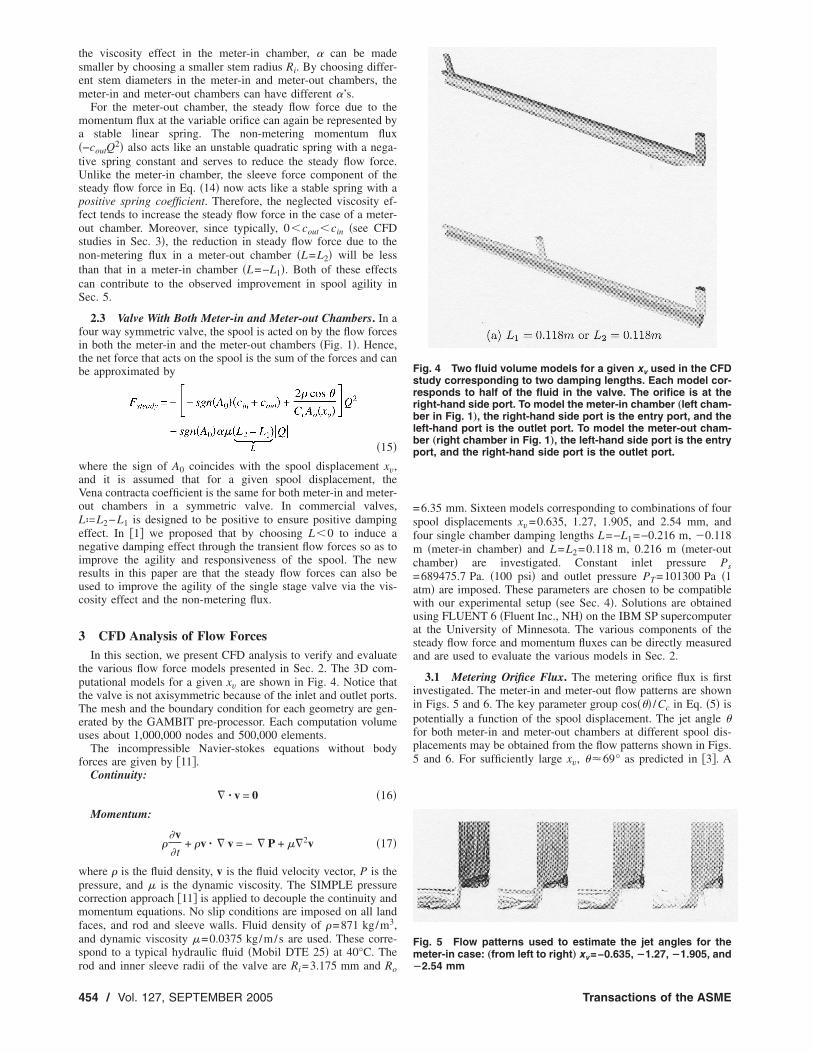
3.1 Metering Orifice Flux. The metering orifice flux is firstinvestigated. The meter-in and meter-out flow patterns are shownin Figs. 5 and 6. The key parameter group cos��� /Cc in Eq. �5� ispotentially a function of the spool displacement. The jet angle �for both meter-in and meter-out chambers at different spool dis-placements may be obtained from the flow patterns shown in Figs.5 and 6. For sufficiently large xv, ��69° as predicted in �3�. A
Fig. 4 Two fluid volume models for a given xv used in the CFDstudy corresponding to two damping lengths. Each model cor-responds to half of the fluid in the valve. The orifice is at theright-hand side port. To model the meter-in chamber „left cham-ber in Fig. 1…, the right-hand side port is the entry port, and theleft-hand port is the outlet port. To model the meter-out cham-ber „right chamber in Fig. 1…, the left-hand side port is the entryport, and the right-hand side port is the outlet port.
Fig. 5 Flow patterns used to estimate the jet angles for themeter-in case: „from left to right… xv=−0.635, �1.27, �1.905, and
�2.54 mm
Transactions of the ASME
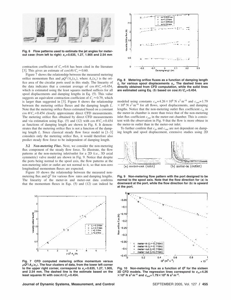
contraction coefficient of Cc=0.6 has been cited in the literature�3�. This gives an estimate of cos��� /Cc�0.60.
Figure 7 shows the relationship between the measured meteringorifice momentum flux and �Q2 /Ao�xv�, where Ao�xv� is the ori-fice area of the circular ports used in this study. The linearity ofthe data indicates that a constant average of cos � /Cc=0.454,which is estimated using the least squares method suffices for allspool displacements and damping lengths in Eq. �5�. This valuesuggests an equivalent contraction coefficient of Cc�0.79, whichis larger than suggested in �3�. Figure 8 shows the relationshipbetween the metering orifice fluxes and the damping length L.Note that the metering orifice fluxes estimated based on a constantcos � /Cc=0.454 closely approximate direct CFD measurements.The metering orifice flux obtained by direct CFD measurementsand via estimation using Eqs. �5� and �12� with cos � /Cc=0.454as functions of damping length are shown in Fig. 8. It demon-strates that the metering orifice flux is not a function of the damp-ing length L. Since classical steady flow force model in �1–3�considers only the metering orifice flux, it would therefore alsopredict steady flow force to be independent of damping length.
3.2 Non-metering Flux. Next, we consider the non-meteringflux component of the steady flow force. To illustrate, the flowpatterns at the non-metering inlet/outlet for a 2D �i.e., 3D axialsymmetric� valve model are shown in Fig. 9. Notice that despitethe ports being normal to the spool axis, the flow patterns at thenon-metering inlet or outlet are not normal to it, so that non-zerolongitudinal momentum fluxes are expected.
Figure 10 shows the relationship between the measured non-metering flux and Q2 for various flow rates and damping lengths.The linearity of the meter-in and meter-out data confirmsthat the momentum fluxes in Eqs. �5� and �12� can indeed be
Fig. 6 Flow patterns used to estimate the jet angles for meter-out case „from left to right… xv=0.635, 1.27, 1.905 and 2.54 mm
Fig. 7 CFD computed metering orifice momentum versus�Q2 /Ao„xv…. The four clusters of data, from the lower left cornerto the upper right corner, correspond to xv=0.635, 1.27, 1.905,and 2.54 mm. The dashed line is the estimate based on the
least squares fit with cos„�… /Cc=0.454.
Journal of Dynamic Systems, Measurement, and Control
modeled using constants cin=4.26106 N s2 m−6 and cout=1.79106 N s2 m−6 for all flows, spool displacements, and dampinglengths. Notice that the non-metering outlet flux coefficient cin inthe meter-in chamber is more than twice that of the non-meteringinlet flux coefficient cout in the meter-out chamber. This is consis-tent with the observation in Fig. 9 that the flow is more obtuse inthe meter-in outlet than in the meter-out inlet.
To further confirm that cin and cout are not dependent on damp-ing length and spool displacement, extensive studies using 2D
Fig. 8 Metering orifice fluxes as a function of damping lengthL, for various spool displacements xv. The dashed lines aredirectly obtained from CFD computation, while the solid linesare estimated using Eq. „5… based on cos„�… /Cc=0.454.
Fig. 9 Non-metering flow pattern with the port designed to benormal to the spool axis. Note that the flow direction for „a… isdownward at the port, while the flow direction for „b… is upwardat the port.
Fig. 10 Non-metering flux as a function of Q2 for the sixteen3D CFD models. The regression lines correspond to cin=4.26
6 2 −6 6 2 −6
Ã10 N s m and cout=1.79Ã10 N s m .
SEPTEMBER 2005, Vol. 127 / 455
�equivalent to 3D axis-symmetric� CFD models with multipleflow rates at each spool displacements and damping lengths wereperformed. Figure 11 shows that cin and cout can be treated asconstants in these 2D cases as well.
3.3 Viscosity Effect. Figure 12 shows Fsleeve, computed fromthe fundamental equations �6� and �13� as a function of �QL forthe 16 test geometries. The linear nature of the curve indicates thatthe laminar and fully developed flow approximations in Eqs. �7�and �14� are accurate. The least squares estimate for the coeffi-cient � is 1106 m−2 and the one computed analytically from Eq.�8� is 0.8106 m−2. Figure 12 shows that these estimates arequite close.
3.4 Total Steady Flow Force. Consider the following expres-sions for the steady flow force that use different approximations:
Fsteady,0 = Fland + Frod �18�
Fsteady,1 = − Fefflux,1 + Fsleeve,1 �19�
Fsteady,2 = − Fefflux,2 + Fsleeve,2 �20�
Fsteady,inviscid = − Fefflux,2 �21�
where Fsteady,0 is the most fundamental, computed directly basedon Eq. �1�; Fsteady,1 is the approach based on the fundamentalmomentum equation in Eqs. �4�, �6�, and �13�; Fsteady,2 is based onthe approximate momentum equations—Eqs. �5�, �7�, �12�, and�14�—using the estimated parameters; Fsteady,inviscid is the estimateof the steady flow forces that neglects viscosity. Notice in Fig. 13shows that Fsteady,0, Fsteady,1, and Fsteady,2 are almost exactly thesame. Both the fundamental and approximate momentum methods
Fig. 11 Estimated cin and cout for various spool displacementsand damping lengths L in a 2D CFD model. Top: Various xv andL=0.15 m. Bottom: Various L and xv=0.645 mm.
to calculate the, steady flow forces are accurate. Furthermore, Fig.
456 / Vol. 127, SEPTEMBER 2005
13 shows that the viscosity effect plays a significant role in deter-mining the steady flow forces. It reduces the steady flow force fornegative damping lengths, while increasing it for positive damp-ing lengths. The extent to which the steady flow force varies in-creases with the damping length.
Figure 14 shows the dependence of the steady flow force foreach meter-in/meter-out chamber on damping lengths according toEq. �20�. Notice the discontinuity of the flow force at L=0. Sincethe damping length L in Fig. 14 is produced using single chamber�i.e., either L1=0 or L2=0 where only one of cin or cout is at playat a time�, the discontinuity is related to the difference betweenthe meter-in and meter-out non-metering flux, �cin−cout�Q2 so thatit decreases for smaller xv �hence Q�. Figure 15 shows the totalsteady flow force for the two-chamber-four-way valve accordingto Eq. �15�. Compared to Fig. 14, no discontinuity is present be-cause both the non-metering inlet and outlet fluxes are simulta-neously present in all damping lengths. Figure 15 also shows thatboth the viscosity and non-metering flux are more significant athigh flow rate. The non-metering effect is illustrated by the paral-lel shift and is given by �cin+cout�Q2. Additional CFD analysis�not shown� reveals that the non-metering flux as a proportion ofthe metering orifice flux will be even larger for axisym-metric�i.e., 2D� valves, than in the 3D axis-symmetric case in Fig. 4.
3.5 Modifying the Non-metering Flux. Since the non-metering fluxes tend to reduce steady flow forces, it would beadvantageous if it can be manipulated by design. One straightfor-ward idea is to change the angle of the non-metering port to thespool axis �8�. Figures 9, 16, and 17 illustrate the differences inflow patterns for three port angles for a 2D �or 3D axis-symmetric� CFD model. Table 1 shows the non-metering flux val-ues for various port angles, normalized by the value for the 0° portangle, meter-in chamber case. It can be seen that the non-meteringflux is susceptible to changes in geometric configuration of thenon-metering port. In particular, by rotating the inlet and outletports in the counterclockwise direction, the non-metering fluxes inboth the meter-in and meter-out chambers increase. If the port isrotated 30° counterclockwise, the sum of the non-metering fluxesof the two chambers increase by 37%, thus having the effect offurther reducing the steady flow force.
Although the port angle affects the non-metering flux, flow pat-
Fig. 12 CFD computed sleeve force Fsleeve as the function of�QL. The sixteen diamond points correspond to the sleeveforces computed from sixteen CFD models, and the dotted lineis the least squares fit. The solid line is calculated from Eq. „7…or Eq. „14… with � computed from Eq. „8….
terns in Figs. 9, 16, and 17 show that the mean angles at which the
Transactions of the ASME
damping length
Fig. 13 Steady flow forces computed from various methods asa function of the orifice displacement. Four different damping
lengths are considered.
Journal of Dynamic Systems, Measurement, and Control
Fig. 14 Steady flow forces as a function of the single chamber
Fig. 15 Steady flow forces and their estimates in a two cham-ber four way valve as a function of the damping length for fourssets of spool displacements. “A” takes into account non-metering flux, “B” does not take into account non-meteringflux. The horizontal bars at L=0 indicate the estimates if vis-cosity effect is ignored.
Fig. 16 Non-metering flow pattern for a 2D CFD model with theport rotated �30° clockwise from the normal direction to thespool axis. Note that the flow direction for „a… is downward at
the port, while the flow direction for „b… is upward at the port.
SEPTEMBER 2005, Vol. 127 / 457
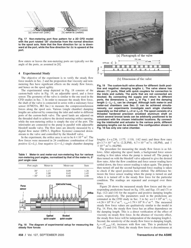
flow enters or leaves the non-metering ports are typically not theangle of the ports, as assumed in �8�.
4 Experimental StudyThe objective of the experiment is to verify the steady flow
force models in Sec. 2 and the proposition that viscosity and non-metering flux have significant effects on the steady flow forces,and hence on the spool agility.
The experimental setup depicted in Fig. 18 consists of thecustom-built valve in Fig. 19, an adjustable spool, and a forcesensor. The geometry of the valve is similar to the one used in theCFD studies in Sec. 3. In order to measure the steady flow force,the shaft of the valve is connected in series with a stationary forcesensor �67M25A, JR3 Inc.� to measure the compression/tensionforces along the spool axis. Various �single chamber� dampinglengths are achieved by connecting the inlet and outlet to differentports of the custom-built valve. The spool lands are adjusted onthe threaded shaft to achieve the desired metering orifice opening,while the non-metering orifice is simply the size of the port. Theinlet/outlet are connected to the pump in parallel with adjustablebleedoff needle valve. The flow rates are directly measured by adigital flow meter �DFS-3, Digiflow Systems� connected down-stream to the valve and controlled by the bleedoff valve.
In the experiment, the orifice area is set to be 610−6 m2. Theflow forces were measured in 24 conditions: combination of fourpositive �L=L2�, four negative �L=−L1� single chamber damping
Fig. 17 Non-metering port flow pattern for a 2D CFD modelwith the port rotated -30° clockwise from the normal directionto the spool axis. Note that the flow direction for „a… is down-ward at the port, while the flow direction for „b… is upward at theport.
Table 1 Meter-in and meter-out non-metering flux for variousnon-metering port angles, normalized by that of the meter-in, 0°port angle case
Port angle Meter-in Meter-out Sum
30° 1.17 0.09 1.260° 1.00 0.45 1.45
30° 1.20 0.80 2.00
Fig. 18 The diagram of experimental setup for measuring the
steady flow forces
458 / Vol. 127, SEPTEMBER 2005
lengths: L= ±236, �175, �118, �62 mm�; and three flow ratesQ=3.710−5 m3/s �2.2LPM�, 6.710−5 m3/s �4LPM�, and 110−4 m3/s �6LPM�.
The procedure for measuring the steady flow forces is as fol-lows. After adjusting the spool lands, a background force sensorreading is first taken when the pump is turned off. The pump isthen turned on with the bleedoff valve adjusted to give the desiredflow rates. After the flow condition and force sensor reading havesettled down, the force sensor reading is taken again. The pump isthen turned off and the second background force reading is takento check if the spool positions have shifted. The difference be-tween the force sensor reading when the pump is turned on andwhen it is turned off is the steady flow force for the particularcondition. The readings are repeated and averaged over threetimes.
Figure 20 shows the measured steady flow forces and the cor-responding predictions based on Eq. �10�, and Eqs. �5� and �7� orEqs. �12� and �14� for the negative and positive damping lengthscases, respectively. The parameters used in the predictions areestimated in the CFD study in Sec. 3 to be: �=1106 m−2, cin=4.26106 N s2 m−6, cout=1.79106 N s2 m−6. The measuredsteady flow force values are qualitatively similar to the model inFig. 14. First, the steady flow force has an affine dependence onthe damping length. This is a direct verification of the effect ofviscosity on steady flow force. In the absence of viscosity effect,the steady flow force will be independent of the damping length L.Second, the sensitivity of the steady flow force to damping length,kLª�Fsteady /�L, increases with flow rate. This is predicted by
Fig. 19 The custom-built valve allows for different „both posi-tive and negative… damping lengths L. The valve sleeve haseleven „11… ports, fitted with quick couplers for connection tothe inlets and outlets. The ports that are not connected areblocked. By connecting the supply and return to differentports, the dimensions L1 and L2 in Fig. 1 and the dampinglength LªL2−L1 can be changed. Although both meter-in andmeter-out chambers „see Sec. 2… can be achieved simulta-neously, our experiments investigate each single chamberseparately so that either L1=0 or L2=0. The spool consists of athreaded hardened precision anodized aluminum shaft onwhich several bronze lands can be arbitrarily positioned to beconsistent with the chosen inlet/outlet locations. By connect-ing the inlet/outlet and actuator to the various ports, differentdamping lengths can be achieved. The configuration shown inFig. 18 has only one valve chamber.
Eqs. �7� and �14�. Third, the steady flow force is discontinuous at
Transactions of the ASME
L=0 with the discontinuity increasing with flow rate. This is dueto the non-metering orifice flux, as discussed in Sec. 3 �i.e., forsingle chamber case, either cin or cout but not both contribute tothe non-metering flux, depending on the sign of L�. Notice alsothat, as predicted, the steady flow force is reduced for negativedamping lengths, and for sufficiently negative damping lengths,the steady flow force becomes marginally stable or even unstable�reverses sign�.
Fig. 21 Relationship between flow force sensitivity to damp-ing length kL, and flow rate Q. The squares correspond to theslopes of the dashed lines in Fig. 20 that are the regressionlines of the experimental data. The dashed line is the curve fit
Fig. 20 Measurements „“squares” and dashed lines… and esti-mation „“triangles” and solid lines… of steady flow forces as afunction of the damping length for various flow rates. Thedashed lines are regression lines of the experimental data as-suming a constant kLªFsteady /�L for each flow rate. Top: Q=2.2 LPM, middle: Q=4.0 LPM, bottom: Q=6.0 LPM.
of the squares, whose slope should be ��.
Journal of Dynamic Systems, Measurement, and Control
In the study of unsteady flow force in a four-way valve in �9�, itwas observed that the flow forces at low frequency �i.e., steadyflow forces� increase with damping lengths. This effect was pre-viously unexplained but is exactly what the new flow force mod-els that include viscosity effect would predict.
Notice that for each Q, the steady flow force can be fitted bytwo straight �dashed� lines �L�0 and L�0� using the same slopekLª�Fsteady /�L, in Fig. 20. The relationship between kL and Q ispredicted by Eqs. �7� and �14� to be kL=��Q where � is thedynamic viscosity. Experimental results in Fig. 21 confirm that kLindeed increases linearly with the flow rate. This implies that, inthe high flow rate applications, negative damping lengths will bemore effective in reducing steady flow forces. In addition, we canquantitatively calculate the parameter � from Fig. 21. The straightdashed line has a slope which should be ��. This gives a value of�=0.978106 m−2 which is close to the values obtained by CFDin Sec. 3 �1.0106 m−2� or via Eq. �8� �0.8106 m−2�.
Despite excellent match in the viscosity effect, there are somesignificant quantitative discrepancies between the experimental re-sults in Fig. 20 and the model. First, the discontinuity at L=0between the meter-in and meter-out chamber is significantly largerthan that predicted by the expected non-metering flux differences.Second, the experimental data tend to be more negative than theprediction, especially when L�0. Extensive effort was spent toinvestigate the source of these disparities. Two limitations of ourexperimental setup have been identified as causes. First, since thevalve lands are machined by hand, it turns out that the areas of thetwo spool lands are different. The area difference was estimatedby measuring the spool force when the closed chamber formedusing the two lands is pressurized. The land at the metering orificewas found to be smaller by �A=0.186 mm2. This leads to an extraorifice-closing force �1��A · P �negative force in the figure� asthe chamber is pressurized. Using the pressure measured by thedigital pressure transducers during the experiments, the steadyforce offset �1 are shown in Table 2.
Second, the shape of the lands need to be considered. To avoidhydraulic locking and to reduce friction between the lands and thesleeve, the lands were intentionally machined to have a 2.5° taperto form a hydrostatic bearing. The effect of the taper can be seenin Fig. 22 where the control volume is different from that in Figs.2 and 3. Modifying Eqs. �1� and �2� accordingly, the spool force of
Fig. 22 Modified control volume of the valve with taperedlands. The metering orifice land area is also smaller than thearea of the left hand side land. The control volume is the gray
colored block.
SEPTEMBER 2005, Vol. 127 / 459
the tapered land valve is
�22�where n is the outward normal vector of the surface, and nx rep-resents the unit vector in the positive x direction. The offset forcedue to the taper, �2, consists of the longitudinal pressure forceapplied on the orifice plane �o-p� and on the side surface �s-l�,respectively. It can be seen that �2�0 for the meter-in case be-cause the first term of �2 is greater than the second term, while�2�0 for the meter-out case because of the opposite effect. Thenumerical values of �2 were obtained via CFD analysis of a 2D�i.e., axis-symmetric 3D� model at various pressure differencesacross the orifice. The �2 values for the 3D axis-asymmetric casewere then estimated from the 2D case with the same pressuredifference, corrected for the port area difference �3D case value isapproximately 50% of the equivalent 2D case value�. The specificvalues for the experimental conditions are listed in Table 2. Thepredicted flow forces after incorporating the offsets �1+�2 matchthe experimental results very closely �Fig. 23�. Even better matchcan be obtained by slightly adjusting �2. The fact that �1 and �2are of different signs for L�0 explains the observation that there
Fig. 23 Measurements „“squares” and dashed lines… and esti-mation „“triangles” and solid lines… of steady flow forces as afunction of the damping length for various flow rates. The esti-mates take into account limitation of the experimental setup viaEq. „22…. The dashed lines are regression lines of the experi-mental data assuming a constant kLª�Fsteady /�L for each flowrate. Top: Q=2.2 LPM, middle: Q=4.0 LPM, bottom: Q=6.0 LPM.
are less discrepancies for L�0 than for L�0 in Fig. 20. In a
460 / Vol. 127, SEPTEMBER 2005
commercial valve, where the lands can be precisely machined, theland area difference is expected to be much smaller, and no taperor a much smaller taper will generally be used. Therefore, inpractice, the �1+�2 correction will not be needed.
5 Effect of Damping Lengths on Spool AgilityThe central hypothesis in �1� is that by configuring the valve to
have a negative damping length, the transient flow force will havean unstable negative damping effect on the spool, thus increasingspool agility. On the other hand, Secs. 2–4 show that negativedamping lengths also decrease the steady flow force via the vis-cosity effect, which would also increase spool agility. In this sec-tion, experimental results are presented to confirm the effect ofdamping length on spool agility as determined by stroking time,and the relative contributions of the transient and steady flowforces for a typical setup.
The experimental setup in Fig. 24 consists of the single cham-ber �meter-out or meter-in� spool valve with adjustable dampinglengths. Unlike the stationary setup in Sec. 4, a solenoid is used tostroke the spool; and a potentiometer is used to measure the spooldisplacement. The solenoid is driven by the current driver circuitin Fig. 25, so that the control voltage Vc applied to the circuitwould determine the solenoid current. A spring is used to push thespool to a fixed initial position where the orifice displacementxv=0. The spool stops when the mobile armature of the solenoidtouches the core. The control of the solenoid and the data acqui-sition system are coordinated by a PC within the Matlab �Math-works, MA� environment via the Matlab’s Realtime Toolbox �Hu-musoft, CZ Rep.�.
Step voltage inputs of Vc=1.6 V �corresponding to solenoidcurrent of 1.45 A� at t=0.5 s are applied for the various damping
Fig. 24 Schematic of the experimental setup used to investi-gate the effect of the damping length on spool agility
Fig. 25 Current driver circuit for solenoid. “Coil” refers to thecoil of the solenoid. The current through the coil is Vc /R in
which R=1.1 is the sensing resistor.
Transactions of the ASME
lengths and the spool displacement trajectories are recorded. Asshown in Fig. 26, as the damping length decreases, it takes lesstime for the spool to travel the full stroke of 4.5 mm �transit time�.In particular, the transit time for L=0.216 m is over 60 ms, whilethe transit time for L=−0.216 m is about 37 ms �Fig. 26� which isabout 40% shorter. The experimental result shows clearly thatdamping length has a significant effect on spool agility. This resultis qualitatively consistent with the effect of damping lengths ontransient flow force �1� as well as with their effects on steady flowforces due to viscosity.
To determine the relative contributions due to transient flowforce or viscosity induced steady flow force reduction, considerthe dynamics of the spool in Fig. 24:
where m is the lumped mass of the spool and the armature of thesolenoid, Fsolenoid is the solenoid force which is a static nonlinearfunction of the current and the displacement �12�, Fspring is thespring force that a function xv. The total work done by the tran-sient flow forces, the solenoid force, and the spring force are
W =�xv�t0�
xv�tf�
�Ftransient + Fsolenoid�xv� + Fspring�xv��dxv
=1
2mxv
2�tf� −�xv�t0�
xv�tf�
Fsteadydxv �24�
where xv�t0� is the initial spool displacement �spool is at rest� andtf are the various sample times when the spool is in motion. xv iscomputed from the trajectory in Fig. 26. For each damping length,xv�t0�
xv�tf�Fsteadydxv can be computed using the steady flow force mod-
els �22� and by assuming a quasi-static condition.The comparison of W and work done by Fsteady for two damp-
ing lengths, L= ±0.216 m, and step voltage input Vc=1.6 V, areshown in Fig. 27. Note that for each xv�tf� and constant voltageVc, the work done by the solenoid and by the spring are identicalbecause the current through the solenoid is constant, andFsolenoid�xv�+Fspring�xv� become a function of xv alone. Therefore,the observed difference in W in Fig. 27 between two dampinglengths is the difference in the work done by transient flow forcesalone. The differences between the Fsteady, on the other hand, isdue to viscosity effect. Note that W is larger for negative damping
Fig. 26 Spool displacement trajectories for various dampinglengths „from left to right: L=0.216, 0.118, �0.118, �0.216 m…,when a step input of Vc=1.6 V is applied at the instant t=0.5 s
lengths than for positive damping lengths indicating extra tran-
Journal of Dynamic Systems, Measurement, and Control
sient flow forces assisting the spool to open. This is also the casefor the work done by the steady flow force, indicating that fornegative damping length, viscosity effect assists valve opening. Inparticular, for large valve openings, the work done contributed bythe viscosity effect of damping lengths on steady flow force is ofa similar magnitude as the work done by transient flow forceeffect. However, for small valve openings, the latter is more sig-nificant. This is consistent with the result in Fig. 21 that the effectof damping lengths on steady flow force is greater at higher flowrates. At least for the valve geometry we have investigated, bothtransient and steady flow force are important considerations forimproving the spool agility.
6 ConclusionIn this paper, we demonstrate that the fluid viscosity and the
non-metering flux are very important in the estimation of thesteady flow forces. On one hand, in the negative damping lengthregion, the steady flow forces, conventionally regarded to be al-ways stabilizing, can be reduced to be marginally stable or un-stable, thus improving the agility of the spool. Paradoxically, us-ing a valve with negative damping lengths, the spool’s agility willimprove as the fluid becomes more viscous. On the other hand,the non-metering flux can be tuned by changing the angle of thenon-metering port to the spool axis, so that the net momentumefflux, which is traditionally regarded to be always stabilizing,could possibly be reduced to be marginally stable or unstable. Theviscosity and the non-metering effects predicted by the proposedmodels and CFD analysis are verified in experiment.
The viscosity and non-metering flux effects generate othervalve design parameters that can be used to improve spool agilityin single stage electrohydraulic valves. Since the steady flow forceis a significant force that the solenoid actuator has to overcome,the reduction of the steady flow force via the viscosity and non-metering effect will be useful for developing high performance
Fig. 27 Work done by the sum of the transient flow forces,solenoid force, and the spring force; and by the steady flowforce, as functions of xv„tf… when step voltage input of Vc=1.6 V is applied, for damping lengths L= ±0.216 m.
single stage valves.
SEPTEMBER 2005, Vol. 127 / 461
Appendix: Detailed Derivation of the ViscosityComponent of the Steady Flow Force
For the valve with geometry in Fig. 2, the sleeve force is fun-damentally given by
Fsleeve,1 = 2 Ro��−�Ld+L1�
0 �vx
�r
r=Ro
dx �A1�
where ��vx /�r�r=Rois the longitudinal velocity gradient in the out-
ward radial �r� direction evaluated at the sleeve wall �r=Ro�. Ifthe friction in the dead space is negligible,
Fsleeve,1 � 2 Ro��−L1
0 �vx
�r
r=Ro
dx . �A2�
For laminar and fully developed flow, it can be shown that �10�
1
r
d
dr�r
dvx
dr� =
1
�
dP
dx�A3�
where P�x� is the pressure. Applying the no-slip conditions thatvx=0 at the rod wall �r=Ri� and the sleeve wall �r=Ro�, the ve-locity distribution can be determined to be
vx =1
4�
dP
dx�r2 − Ro
2 +Ri
2 − Ro2
ln�Ro/Ri�ln
r
Ro �A4�
Since
−�Ri
Ro
2 vxdr = Q ,
�vx /�r can be expressed as a function of Q so that � in Eq. �7� isgiven by
� =4�2Ro
2 ln�Ro/Ri� + Ri2 − Ro
2��Ro
4 − Ri4�ln�Ro/Ri� − �Ri
2 − Ro2�2 . �8�
Nomenclature� � viscosity related geometry coefficient
�1 � land area difference compensation�2 � land tapers compensation
�sleeve � wall stresses on the sleeve�rod � wall stresses on the rod
Al � annular area of the left landAo � orifice areaAr � annular area of the right landCc � Vena contracta contraction coefficientcin � meter-in chamber non-metering outlet flux
Fefflux � net momentum effluxFland � pressure force acting on the landsFrod � viscous force acting on the rod
Fsleeve � viscous sleeve force acting on fluidFsolenoid � solenoid force
Fspring � spring forceFspool � fluid flow force acting on spool
Fsteady � steady flow forceL � damping length
L1 � meter-in chamber damping lengthL2 � meter-out chamber damping lengthLd � dead space distancen � unit vector outward normal to surface
nx � positive x unit vectorkL � steady force sensitivity to damping lengthPl � pressure on the left landPr � pressure on the right landQ � flow rateP � fluid pressureRi � radius of the rodRo � radius of the sleevev � fluid velocity vector
vx � longitudinal fluid velocityW � total work by solenoid, spring, and transient
flow forces
References�1� Krishnaswamy, K., and Li, P. Y., 2002, “On Using Unstable Electrolydraulic
Valves for Control,” ASME J. Dyn. Syst., Meas., Control, 124�1�, pp. 182–190.
�2� Blackburn, J. F., Reethof, G., and Shearer, L. L., 1910, Fluid Power Control,MIT, Cambridge.
�3� Merritt, H. E., 1967, Hydraulic Control System, Wiley, New York.�4� Borghi, M., Milani, M., and Poluzzi, R., 2000, “Stationary Axial Flow Force
Analysis on Compensated Spool Valves,” Int. J. Fluid Power, 1�1�, pp. 17–25.�5� Yang, R., 2003, “Hydraulic Spool Valve Metering Notch Characterization Us-
ing CFD,” in ASME Fluid System Technology Division Publication - 2003International Mechanical Engineering Congress, vol. 10, pp. 11–17.
�6� Mookherjee, S., Acharyya, S., Majumdar, K., and Sanyal, D., 2001, “Static-Performance Based Comuter-aided Design of a DDV and its Sensitivity Analy-sis,” Int. J. Fluid Power, 2�2�, pp. 47–63.
�7� Del Vescovo, G., and Lippolis, A., 2003, “Three-dimensional Analysis of FlowForces on Directional Control Valves,” Int. J. Fluid Power, 4�2�, pp. 15–24.
�8� McCloy, D., and Martin, H. R., 1980, Control of Fluid Power, Analysis andDesign, 2nd ed., Ellis Horwood, West Sussex.
�9� Nakada, T., and Ikebe, Y., 1980, “Measurement of the Unsteady Axial FlowForce on a Spool Valve,” in Proceedings of the IFAC Symposium - Pneumaticand Hydraulic Components and Instruments in Automatic Control, Warsaw,Poland. IFAC, May 1980, pp. 193–198.
�10� Munson, B. R., Young, D. F., and Okiishi, T. H., 1998, Fundamentals of FluidMechanics, 3rd Edition, Wiley, New York.
�11� Tannehill, J. C., Anderson, D. A., and Pletcher, R. H., 1997, ComputationalFluid Mechanics and Heat Transfer, Taylor and Francis, Philadelphia.
�12� Xu, Y., and Jones, B., 1997, “A Simple Means of Predicting the DynamicResponse of Electromagnetic Actuators,” Mechatronics 7�7�, pp. 589–598.