Using the SPAC Microtremor Method to Identify 2D Effects · Using the SPAC Microtremor Method to...

Using the SPAC Microtremor Method to Identify 2D Effects

and Evaluate 1D Shear-Wave Velocity Profile in Valleys

by M. Claprood, M. W. Asten, and J. Kristek

Abstract The requirement of a layered-earth geology is a restrictive assumptionwhen using the spatially averaged coherency spectra (SPAC) method. Numericalsimulations of microtremors and SPAC observations recorded in the Tamar paleoval-ley, Launceston (Tasmania, Australia), are used to assess the potential of the SPACmethod to identify two-dimensional (2D) effects and evaluate one-dimensional(1D) shear-wave velocity (SWV) profile in a valley environment. The Tamar Valleyis approximately 250 m deep by 700–1000 m wide. It is filled with soft sedimentsfrom the Tertiary and Quaternary periods above hard dolerite bedrock of Jurassic age.

Observed coherency spectra of the vertical component are analyzed at two sites inthe Tamar Valley; using two 50-m-radius centered triangular arrays above the deepestpoint of the valley at site DBL, and above the east flank of the valley at site RGB.Simulated and observed coherency spectra suggest the propagation of Rayleigh wavesof first higher mode at the SV frequency of resonance of the Tamar Valley affectsthe coherency spectra recorded with pairs of sensors perpendicular to the valley(transverse-COH). Simulated and observed coherency spectra recorded above thedeepest point of the valley (site DBL) with pairs of sensors parallel to the valley axis(axial-COH) are not affected by these edge-generated Rayleigh waves and agree wellwith the theoretical coherency spectrum computed from the preferred 1D SWV profile.

The simulated and observed results from this paper suggest that differencesbetween the observed axial-COH and transverse-COH give an indication of the exis-tence of the 2D buried valley. Results also suggest that the observed coherency spectrarecorded on pairs of sensors oriented parallel to the valley axis can provide a reliableevaluation of a 1D SWV profile above the deepest point of a deep and narrow valley,such as the Tamar Valley.

Introduction

Microtremor survey methods to evaluate the shear-wavevelocity (SWV) profile at specific sites, using the constantambient vibrations of the ground (referred to as microtre-mors) generated by human activities (at frequency f ≥ 1 Hz)or natural phenomena (at f ≤ 1 Hz) as the source of energy(Okada, 2003) are gaining in popularity. The microtremorsurvey methods are ideally suited for urban environment;they are noninvasive, and their source of energy is continu-ous in proximity to urban agglomerations. An importantproportion of microtremor energy is associated with the pro-pagation of surface waves (Aki, 1957; Capon, 1969; Horike,1985; Tokimatsu, 1997; Okada, 2003; Bonnefoy-Claudetet al., 2006), with fundamental mode Rayleigh waves dom-inating. The dominance of fundamental mode Rayleighwaves is a function of several factors, such as the complexityof SWV structure (Tokimatsu et al., 1992). This hypothesisis important when dealing with the vertical component of

microtremors, which, in the absence of anisotropy, are onlypresent in Rayleigh surface waves (Udías, 1999).

Different processing techniques have been developedto evaluate SWV structures from the frequency dispersivevelocity curves of microtremor propagation. The mostcommon array-based microtremor methods are the spatialautocorrelation method developed by Aki (1957), alsotermed the spatially averaged coherency spectra (SPAC)method (Asten, 2006a); the frequency–wavenumber (FK)method introduced by Toksöz and Lacoss (1968), with twoprocessing algorithms developed by Lacoss et al. (1969) andCapon (1969); and the multiple signal classification (MUSIC)method presented by Schmidt (1986) and Goldstein andArchuleta (1987). Alternative SPAC processing include thecenterless circular array method introduced by Cho et al.(2004, 2006, 2008) and the single circular array methodintroduced by García-Jerez et al. (2008). By recording syn-thetic ambient noise with a dense array of sensors, Wathelet

826

Bulletin of the Seismological Society of America, Vol. 101, No. 2, pp. 826–847, April 2011, doi: 10.1785/0120090232

et al. (2008) concluded there is no significant difference inthe evaluation of SWV profile with the FK or SPAC method.

The microtremor survey methods require the hypothesisof temporal and spatial stationarity of the microtremor wavefield, so it can be treated as a stochastic process (Aki, 1957).This hypothesis is generally valid when recording long (butstill less than 1 hr) microtremor time series, using an arraywith an aperture smaller than one or two kilometers (Toksöz,1964). The temporal and spatial stationarity of microtremorsis essential to validate because unstationarity on the powerspectra makes them time-dependent and impossible to treatas a simple function of frequency (Toksöz, 1964). By record-ing microtremors over a long period of time with an array ofsensors, microtremors can be analyzed as an assemblage ofcoherent waves traveling in various directions and coveringan extended interval of frequencies.

An important hypothesis to consider when using array-based microtremor survey methods is that all sensors ofthe array must sample the same geology. This hypothesisrestricts the use of microtremor survey methods to regionswhere the geology can be approximated by a layered earth.This requirement is very restrictive in the evaluation of SWVat specific sites, and several authors have evaluated the useof the microtremor survey methods above more complexgeology. For example, several studies used single-stationmicrotremor observations, such as the standard spectral ratio(SSR) and horizontal-to-vertical spectrum ratio (HVSR), toidentify the modes and frequencies of resonance that developinvalleys (Field, 1996; Steimen et al., 2003;Uebayashi, 2003;Roten et al., 2006). While some authors have used HVSRobservations to evaluate SWV profiles (Arai and Tokimatsu,2004), Asten et al. (2002) and Chávez-García et al. (2007)demonstrated that single-station microtremor observationsshow poor resolution in evaluating SWV profile and mostoften require a priori knowledge of the velocity structurefor site resonance study in valley environments.

Some authors have developed methodologies to usearray-based microtremor observations in complex geology.Cornou et al. (2003a, 2003b) used the MUSIC algorithm withHVSR observations to identify the wave field associated withsite amplification in the Grenoble Valley (France), using anextensive array of 29 three-component seismometers and atotal array aperture of 1 km. Hartzell et al. (2003) used theFK and MUSIC methods to detect edge-generated surfacewaves with a dense array of 52 sensors in the Santa ClaraValley (U.S.A.), using site response spectra from earthquake-generated motion to evaluate the SWV profile. Roten et al.(2006) and Roten et al. (2008) used the FK method to iden-tify the expected modes of resonance in the Rhône Valley(Switzerland); and Roten and Fäh (2007) evaluated the SWVprofile in the Rhône Valley, using a joint inversion on thevelocity dispersion curve obtained with the FK methodand two-dimensional (2D) resonance frequencies observedon an SSR profile. Recently, Picozzi et al. (2009) used high-frequency seismic noise tomography to image shallow

structural heterogeneities with an array of 21 geophonesat the Nauen test site in Germany.

The SPAC method requires a broad azimuthal distribu-tion of energy sources to achieve best results (Asten, 2003,2006a). This particularity is of interest when recording am-bient seismic noise in a urban environment because citiesprovide microtremor sources from various and unknownorigins. The FK method is more reliable when a preferentialsource of microtremor energy is identified. The need for awide azimuthal source distribution is an important require-ment in order to obtain reliable results with the SPAC method.Results obtained by Cho et al. (2004, 2006a) and Asten(2003, 2006a) showed a departure between the observed andtheoretical coherency spectra with limited source azimuthsampling. This outlines the importance of verifying thesource distribution of the microtremor wave field in theSPAC method flowchart (Aki, 1957).

The SPAC method requires fewer sensors than the FKmethod to achieve similar resolution (Henstridge, 1979;Kudo et al., 2002; Chávez-García et al., 2005; Okada, 2006),reducing human labor and equipment and simplifying thelogistics of field data acquisition. It also offers better resolu-tion at low frequency (corresponding to deep material) forthe same array size (Asten, 1976; Okada, 2003; Hartzellet al., 2005; Claprood and Asten, 2009a), which justifiesthe deployment of smaller arrays to achieve good resolutionat depth. Because SPAC arrays are constrained to regulararray geometry (which can be difficult to achieve in an urbanenvironment), the smaller dimensions of the array and theuse of fewer sensors for the SPAC method are advantageouswhen deploying the equipment in a city.

The approximation of a layered-earth geology is animportant restriction when using the SPAC method. To thebest of our knowledge, little work has been done to analyzethe capabilities of the SPAC method in 2D environments. Thispaper presents an alternative approach to the FK method in2D environments, profiting from the recognized advantagesof the SPAC method (fewer sensors and smaller array geome-try) and quantifying perturbations on SPAC data induced bydepartures from the usual assumption of layered geology.The objectives are (1) to recognize such perturbations by op-timizing the direction between sensors and (2) to analyze thepotential of SPAC observations to evaluate one-dimensional1D SWV profiles in 2D environments. Microtremor observa-tions were recorded in the city of Launceston (Tasmania,Australia), where the presence of the Tertiary-age TamarValley has been outlined, in-filled with soft sediments thatvary rapidly in thickness from 0 m to 250 m over a fewhundreds of meters.

Geophysical Settings

Information on the geology of Launceston is availablefrom unpublished maps from Mineral Resources Tasmania,borehole logs held by Launceston City Council, and a gravitysurvey completed by Leaman (1994). The geological map of

Using the SPAC Microtremor Method to Identify 2D Effects and Evaluate 1D Shear-Wave Velocity Profile 827

Launceston presented in Figure 1 outlines the rapid changesin surface geology in the central business district of Launces-ton, with the geological interpretation of two gravity profilesrecorded across the valley.

The bedrock at Launceston comprises dense, fractured,and weathered Jurassic dolerite (Fig. 1a, zone a), whichprovides reduced seismic risk and excellent foundation con-ditions (Leaman, 1994). It is covered by poorly consolidatedmaterials (i.e., clays, sands, conglomerates, silts, and fills),which can be compressible, water saturated, plastic, and oflow density. Quaternary alluvial sediments (silts, gravels,fills) were deposited in the valley floor and other marshyareas near sea level (Fig. 1a, zones d and e). These sedimentshave poor cohesion and negligible strength, and they may bethixotropic. Low density Tertiary sands and clays fill theancient valley systems beneath Launceston (Fig. 1a, zones f).The gravity interpretation of Leaman (1994) identified twopaleovalley systems in Launceston: the Tamar paleovalleyand the North Esk paleovalley, both trending in a north–

northwest to south–southeast direction. Interpretation of thegravity survey indicates that the Tamar Valley has a width of700–1000 m and a maximum depth of approximately 250 m(Fig. 1b). The Tamar Valley is the focus of our researchbecause it is more continuous and better defined than theNorth Esk Valley.

SPAC Microtremor Method

Microtremors are recorded with an array of geophonesto evaluate the coherency spectrum between all pairs ofsensors in the array. Spatially averaged coherency spectraare then computed for multiple interstation separations byazimuthal averaging. When recording microtremors fromall sources and directions with an array of n sensors azimuth-ally distributed at distance r from a center sensor, the com-plex coherency spectrum Cjc�f� evaluated by each pair ofsensors is computed as:

Figure 1. (a) Map of surface geology of Launceston (modified from Mineral Resources Tasmania). The map is divided into six zonesdelimited by thick black lines. Triangles are the location of SPAC microtremor observations at sites DBL and RGB. Dashed lines indicate thelocation of two gravity profiles from Leaman (1994), presented in panel (b). The bottom of (b) shows the centered triangular SPAC arraygeometry with interstation separations r1 and r2. The color version of this figure is available only in the electronic edition.

828 M. Claprood, M. W. Asten, and J. Kristek

Cjc�f� � expfikrjc cos�θjc � ϕ�g; (1)

where i is the imaginary unit number; k is the spatial wave-number at frequency f; rjc is the interstation separation ofthe jth sensor relative to the center sensor c, with azimuthθjc; and ϕ is the propagation azimuth of a single plane waveacross the array (Asten, 2006a). When considering an infinitenumber of sensors positioned around a center sensor, theintegration of coherencies Cjc�f� with azimuth leads to thespatially averaged coherency spectrum C�f� (Aki, 1957;Okada, 2003):

C�f� � 1

2π

Z2π

0

expfikr cos�θ � ϕ�gdθ; (2)

which can be expressed as the Bessel function of the firstkind and zero order J0 of variable rk:

C�f� � J0�kr� � J0

�2πfrV�f�

�; (3)

where V�f� is the surface wave velocity dispersion functionof a layered-earth model for which the 1D SWV profile isevaluated.

Aki (1957) demonstrated the possibility of usingthe horizontal components of a microtremor wave field toresolve for the Rayleigh and Love wave dispersion curves,gaining constraints on the SWV profile. Köhler et al. (2007)and Fäh et al. (2007) presented the advantages of the addi-tional information gained about Love waves when using thethree-component SPAC and FK methods, respectively. For itssimpler processing, the traditional SPAC method (using thevertical component only) is used in this paper.

Modifications to the conventional SPAC processing havebeen developed to permit its use with arrays that deviate fromthe standard circular and equidistant configuration (Bettiget al., 2001; Ohori et al., 2002; Cho et al., 2004; Köhler et al.,2007). This idea was originally proposed by Aki (1957) andmathematically demonstrated by Capon (1973), who provedthat identical results are obtained when using either a singlepair of sensors to record an omnidirectional wave field or anarray of n sensors to record one single plane wave of uniqueazimuth. The integration of complex coherency spectra isadapted to sum over the sources azimuth ϕ, with the sensorsorientation θ fixed.

Some authors proposed using a single pair of sensors toevaluate the coherency spectrum, replacing the spatial aver-aging by temporal averaging and increasing the length of themicrotremor time series (Aki, 1957; Morikawa et al., 2004;Chávez-García et al., 2005). By increasing the recordingtime, the probability to respect the azimuthal distribution ofmicrotremor sources increases considerably, which improvesthe reliability of SPAC observations recorded with a pair ofsensors. Following the recommendations from Okada (2006)and Claprood and Asten (2010), we restrict the analysis to

frequencies up to the first minimum of the Bessel functionwhen using a single pair of sensors.

The domain of validity of the frequency interval tointerpret SPAC observations with an array of sensors is stilldebated in the literature. Henstridge (1979) first proposed torestrict the valid frequency interval to 0:4 ≤ rk ≤ 3:2, whererk is the argument of the Bessel function (r is the interstationseparation, k is the wavenumber). The upper limit corre-sponds to the Nyquist frequency, which limits the interpreta-tion at high frequency. Okada (2006) further investigated thatupper limit, suggesting it is restricted by the number of sen-sors in the array and approximately corresponds to the firstminimum of the theoretical Bessel function. Asten (2006a,2006b) suggested that the multiple mode SPAC method(MMSPAC) can be reliable to frequencies as high as rk≃ 20

when the microtremor wave field has adequate azimuthalcoverage and that the upper frequency should be determinedby analyzing the microtremor wave field. The upper fre-quency limit was pushed to extreme limits by Ekström et al.(2009). We followed the MMSPAC philosophy in this studywhen using the spatially averaged coherency spectra, select-ing the interval of valid frequencies on a case-by-casescenario. The valid frequency range is identified on eachselected site on the coherency spectra.

Field Procedure

Microtremor observations were recorded in October2007 in the city center of Launceston, using four three-component Guralp CMG-3ESP 30-s and 60-s periodgeophones. Coherency spectra are observed at two separatesites, DBL and RGB, located within the assumed limits ofthe Tamar Valley (Fig. 1a). SPAC observations were recordedwith time series of 20–30 minutes, sufficient to ensurereliability in the observed coherency spectra computed witha limited number of sensors (Chávez-García and Rogríguez,2007; Chávez-García et al., 2007; Claprood andAsten, 2010).The time series are divided into time segments of 80 secondswith 50% overlap, which are weighted with a Hanning belland then fast-Fourier transformed in the frequency domainto obtain the raw spectra Si�f� of microtremor energy at everysensor i. The coherency spectrum between each pair ofsensors �i; j� is computed using the equation:

Cij�f� �Si�f�S�j �f��

Si�f�S�i �f�Sj�f�S�j �f�q ; (4)

where Cij�f� is the complex coherency and * denotes thecomplex conjugate. Complex coherency spectra are averagedover all time segments to yield the temporally averagedcoherency spectrum at each pair of sensors.

Spatially averaged coherency spectra are computed byaveraging over azimuth for interstation separations r1 and r2,available from the centered triangular arrays used in Laun-ceston (Fig. 1b, bottom). The MMSPAC method is followed


to interpret SPAC observations because of its increasedprecision in the evaluation of SWV profiles. The MMSPACmethod also helps at the recognition of higher modes ofpropagation and justifies the use of fewer sensors and arraysof smaller dimensions. Asten (2005), Roberts and Asten(2005), and Stephenson et al. (2009) presented case studiesin which the advantages of the MMSPAC method areoutlined.

The real component of observed coherency spectra isdirectly fit to the theoretical coherency spectrum J0 byleast-square optimization of successive forward modeling(Herrmann, 2002) to evaluate the SWV profiles without eval-uating the surface wave velocity dispersion function. Astenet al. (2004) indicated that the direct fit of coherency spectraensures minimal loss of information when evaluating theSWV profile. Assuming the predominance of the fundamen-tal mode of propagation of Rayleigh-type surface wave, thefit between the observed and inverted theoretical coherencyspectra is quantified by minimizing the mean square of re-siduals (MSR). The MSR is obtained by dividing the sum ofthe square of residuals (SSR) between observed and theore-tical coherency spectra by the length of the frequency vector.

The MSR is used as an alternative to the SSR tradition-ally employed to compare observations to theoreticalmodels. The MSR was found to be the preferred option tocompare observed coherency spectra computed on differentfrequency intervals (Claprood and Asten, 2010). The MSR isinsensitive to the length of the frequency interval while theSSR varies proportionally with the length of the frequencysupport. When comparing two vectors of the same length,results analyzed with the MSR are equivalent to resultsanalyzed with the SSR. A sensitivity study was completed toanalyze the precision and uniqueness of the preferred SWVprofile evaluated.

Asten (2006a) suggested analyzing the behavior of theimaginary component of the coherency spectrum by separat-ing it into a smoothed and roughened components. Anycyclic behavior of the smoothed imaginary component givesindication about the distribution of the microtremor wavefield; while the root mean square of the roughened imaginarycomponent rmsIm is an evaluation of statistical noise on themicrotremor observations.

We propose the hypothesis that the presence of theTamar Valley impacts the observed coherency spectrum dif-ferently, depending on the orientation of the pair of sensorsfrom which it is computed. Coherency spectra recorded bypairs of sensors oriented axially and transverse to the valleyaxis are likely to present the most significant differences.This will affect the reliability of the SWV profile if tradition-ally computed from the spatially averaged coherency spec-trum. By analyzing the coherency spectra observed fromeach pair of sensors of varying azimuth (Claprood and Asten,2010), we study the spatial distribution of the microtremorwave field and the valid range of frequencies at sites DBLand RGB. The MSR computed between the observed coher-ency spectrum on each pair of sensors and the theoretical

coherency spectrum is used to quantitatively assess the reso-lution of the coherency spectra recorded by pairs of sensorsof different azimuth. It is an alternative to the FK methodto evaluate the azimuth distribution of the microtremorwave field when using a limited number of sensors to recordmicrotremors.

Having access to only four low-frequency seismometers,coherency spectra were successively recorded with twocentered triangular arrays of different orientations to form anonuniform hexagonal array at each site. The first array wasoriented with the pair of sensors XA1 (X is the centersensor, A1 is the first sensor on the array circumference)parallel to the axis of the Tamar Valley (azimuth θ1 � 135°or 315° relative to geographic true north). The second arrayis orientedwith the pair of sensorsXA2 transverse to thevalleyaxis (azimuth θ2 � 45° or 225°). The orientation of eacharray is shown in Figure 2. We use the term “axial-COH”to designate the coherency spectrum recorded with a pair ofsensors oriented parallel to the valley axis and “transverse-COH” for the coherency spectrum recorded with a pair ofsensors perpendicular to the valley axis. The spatially aver-aged coherency spectra on interstation separations are referredto as SPAC and are computed from the average of coherencyspectra recorded from both arrays at each site.

Site DBL

The site DBL (detention basin of Launceston) wasselected for its assumed location above the deepest part ofthe Tamar Valley (Fig. 1a). Sensors were positioned on foot-paths of secondary roads with light traffic to reduce thestatistical noise envelope on SPAC observations. Two 50-m-radius centered triangular arrays were used at site DBL. Thefirst array was oriented with the pair of sensors XA1

parallel to the valley axis (θ1 � 315°), and the second arraywas oriented with the pair of sensors XA2 transverse to thevalley axis (θ2 � 45°).

−500 −250 0 250 500

−250

0

250

distance X (m)

dist

ance

Y (

m) XA1 = axial−COH

XA2 = trans.−COH

XC2

XC1

XB2

XB1

Figure 2. Orientation of two centered triangular arrays used inLaunceston, with the pair of sensors XA1 oriented parallel to thevalley axis (axial-COH), and XA2 perpendicular to the valley axis(transverse-COH). Thick dashed lines are the outlines of the valley.


The temporal stationarity in the microtremor wave fieldis increasingly important when using a limited number ofsensors to record SPAC observations. The temporal stabilityof the microtremor wave field recorded at Launceston isimproved by the removal of time segments presenting tran-sient or abnormal behavior (Margaryan et al., 2009). A totalof Ms � 15 time segments were used for array 1, and Ms �21 for array 2 at site DBL. Figure 3 presents the power spec-tra recorded at site DBL at sensors X and A from both arrays,for all time segments used in the interpretation and their timeaveraged power spectra.

The similarity of the power spectra on all time segmentsfrom each sensor, more obvious for f ≤ 2 Hz, proves thetemporal stability of microtremor propagation at site DBL;which was improved by the removal of transient time seg-ments. The decrease in power spectra observed at approxi-mately 1.0 Hz could be induced by a filtering effects oflow-velocity sediments on vertical motion (Scherbaum et al.,2003). This filtering effect is also observed on the HVSRcurve, which shows a broad peak for 0:8 Hz ≤ f ≤ 1:2 Hz).

The coherency spectra observed on all pairs of sensorsand interstation separations of both arrays at site DBL arepresented in Figure 4 on the frequency interval consideredreliable to evaluate the SWV profile with SPAC at thissite (0:75 Hz ≤ f ≤ 11:5 Hz).

Visual analysis of the observed coherency spectra givesus some knowledge about the source distribution of themicrotremor wave field. We observe little variability betweenthe observed coherency spectra on pairs of sensors of differ-ent orientations for f ≤ 2:0 Hz. This suggests the micro-tremor wave field has adequate azimuthal distribution tocompute coherency spectra with pairs of sensors at theselow frequencies. The increased variability of the observedcoherency spectra with azimuth of the pair of sensors for f >2:0 Hz suggests the azimuthal averaging of observed coher-ency spectra is required to validate the spatial stationarity ofthe microtremor wave field at these higher frequencies. Thesource distribution at site DBL was studied in detail inClaprood and Asten (2010) by analyzing the variability ofcoherency spectra recorded on pairs of sensors oriented atdifferent azimuths and comparing with SPAC on interstation

separations. A frequency–wavenumber analysis conductedwith the same two 50-m centered triangular arrays at siteDBL (not presented) agrees well with the results determinedby the observed coherency spectra at high frequencies.FK plots, however, have poor resolution to detect the direc-tion of microtremor energy sources at frequencies lowerthan 1.6 Hz.

Site RGB

The rugby ground of Launceston (site RGB) isassumed to be located above the eastern flank of the TamarValley. SPAC observations at this site provide additionalinformation about the soft sediments filling the Tamar Valley.This location was also chosen to test the SPAC method over adipping bedrock interface. Two 50-m radius centered trian-gular arrays were laid out in the rugby ground, with the pairof sensors XA successively oriented parallel (θ1 � 315°) andperpendicular (θ2 � 45°) to the valley axis. SPAC observa-tions were recorded with larger arrays at site RGB(r1 � 140 m), but the high level of statistical noise restrictsthe analysis of coherency spectra recorded with these largerarrays. Figure 5 presents the power spectra recorded at siteRGB on sensors X and A from both arrays.

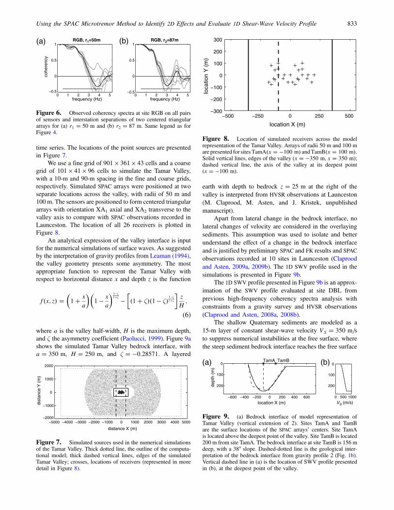
The interpretation of SPAC observations is conducted onthe frequency interval 0:5 Hz ≤ f ≤ 4:25 Hz. The increasein power spectra at low frequency (f ≤ 0:5 Hz) on array 2is unexplained but does not impact the interpretation becauseit falls outside the valid frequency interval. The power spec-tra at some sensors (X1, A1) presents some variability at highfrequencies, which suggest temporal nonstationarity of themicrotremor wave field. The frequency interval upper limitwas fixed at 4.25 Hz to validate the hypothesis of temporalstationarity of microtremors at site RGB. The azimuthaldistribution of microtremor wave field is also verified at siteRGB by analyzing the coherency spectra recorded on allpairs of sensors and interstation separations. The observedcoherency spectra are presented in Figure 6.

The observed coherency spectra present some differ-ences, depending on the azimuth of the pair of sensors theyare computing. As previously analyzed in Claprood andAsten (2010), the microtremor wave field contains energy

DBL, X2

frequency (Hz)

DBL, A2

frequency (Hz)

10−1100

100

101

101 10−1 100 10110−1 100 10110−1 100 101

102

100

101

102

DBL, X1

frequency (Hz)

DBL, A1

frequency (Hz)

Figure 3. Power spectra recorded at site DBL. (Two left panels) Power spectra from array 1 at sensors X1 and A1 on Ms � 15 timesegments. (Two right panels) Power spectra from array 2 at sensors X2 and A2 onMs � 21 time segments. Gray lines, power spectra on eachtime segment; black lines, time averaged power spectra (logarithmic axis).


propagating from a restricted azimuth at site RGB forf ≥ 2:0 Hz. The Tamar River and the busy Bathurst Street,located at approximately two array radii from the arraycenter, are responsible for the restricted azimuth of themicrotremor wave field. The variability of the observed co-herency spectra is significantly reduced at lower frequency.The spatial averaging of coherency spectra on both intersta-tion separations helps to significantly reduce the effect of therestricted azimuth distribution of the microtremor wave fieldat high frequency.

This analysis of the microtremor wave field was essen-tial to better distinguish possible 2D effects from the valleyand localized sources of microtremor. While the variability ofthe microtremor wave field at higher frequencies complicatesthe identification of 2D effects, it is suggested from theresults of numerical simulations shown in the next sectionthat 2D effects from the valley are occurring at frequencieslower than 2 Hz and could thus be identified on observedcoherency spectra because the microtremor source distribu-tion is more stable at these low frequencies.

We analyze the limit of resolution of the array geometry(r1 � 50 m, r2 � 87 m) deployed at both sites by comput-ing the minimum frequency resolvable on both interstationseparations following Henstridge (1979) criteria: 0:4 ≤ rkand using equation (3):

f � 0:4Vmax�f�2πr

; (5)

where Vmax�f� is the maximum Rayleigh-wave velocityestimated at 880 m=s for the Tertiary sediments in-fillingthe valley (Michael-Leiba, 1995). Using equation (5), theminimum frequency resolvable at sites DBL and RGB isestimated at 1.12 Hz for interstation separation r1 � 50 mand 0.64 Hz for r2 � 87 m.

Numerical Simulations

Numerical simulations of microtremors in complexgeological media are used to better control the parametersimpacting the recording of coherency spectra in a 2D envi-ronment and to compare with coherency spectra observed atsites DBL and RGB in the Tamar Valley. The program pack-age NOISE developed within the European Site EffectsAssessment using Ambient Excitations (SESAME) project isused for the computation of seismic noise (microtremors)propagation in 3D heterogeneous geological structures witha planar free surface, from surface and near-surface randomsources (Moczo and Kristek, 2002; J. Kristek, P. Moczo, andM. Kristekova, unpublished manuscript). The package isdivided into two main programs: Ransource for the randomspace–time generation of microtremor point sources andFdsim for the computation of seismic wave fields in 3D het-erogeneous geological structures (Kristek et al., 2002; Moc-zo et al., 2002; Kristek et al., 2009; Moczo et al., 2007).

The source time functions were selected to be 50%deltalike signals (approximation to Dirac delta distribution),and 50% pseudomonochromatic functions of random dura-tion and frequency. All source time functions were band-pass-filtered in the frequency range 0.4–3.0 Hz. The lowerfrequency boundary is selected to avoid the propagationof wavelengths larger than the size of the computationalmodel. The upper frequency boundary is determined bythe chosen grid spacing. A dense sampling of the shortestwavelengths of the wave field is required to avoid grid dis-persion. A total of 79,442 point sources were space–time ran-domly distributed at the surface of a 9000 m × 3600 m gridover 100,000 time levels (dt � 0:0014 s), generating a 140-s

0 2 4 6 8 10 12−0.5

0

0.5

1DBL, r1=50m

cohe

renc

y

frequency (Hz)

(a)

0 2 4 6 8 10 12−0.5

0

0.5

1DBL, r2=87m

frequency (Hz)

(b)

Figure 4. Observed coherency spectra at site DBL on all pairsof sensors and interstation separations of two centered triangulararrays for (a) r1 � 50 m and (b) r2 � 87 m. Gray lines, coherencyspectra recorded on pairs of sensors; thick black lines, spatiallyaveraged coherency spectra; solid line (at bottom of each graph),valid frequency interval at site DBL.

100

101

10−1 100 101 10−1 100 10110−1 100 10110−1 100 101

102

100

101

102

RGB, X1

frequency (Hz)

RGB, A1

frequency (Hz)

RGB, X2

frequency (Hz)

RGB, A2

frequency (Hz)

Figure 5. Power spectra recorded at site RGB. (Two left panels) Power spectra from array 1 at sensors X1 and A1 on Ms � 38 timesegments. (Two right panels) Power spectra from array 2 at sensors X2 and A2 on Ms � 32 time segments. Same legend as for Figure 3.


time series. The locations of the point sources are presentedin Figure 7.

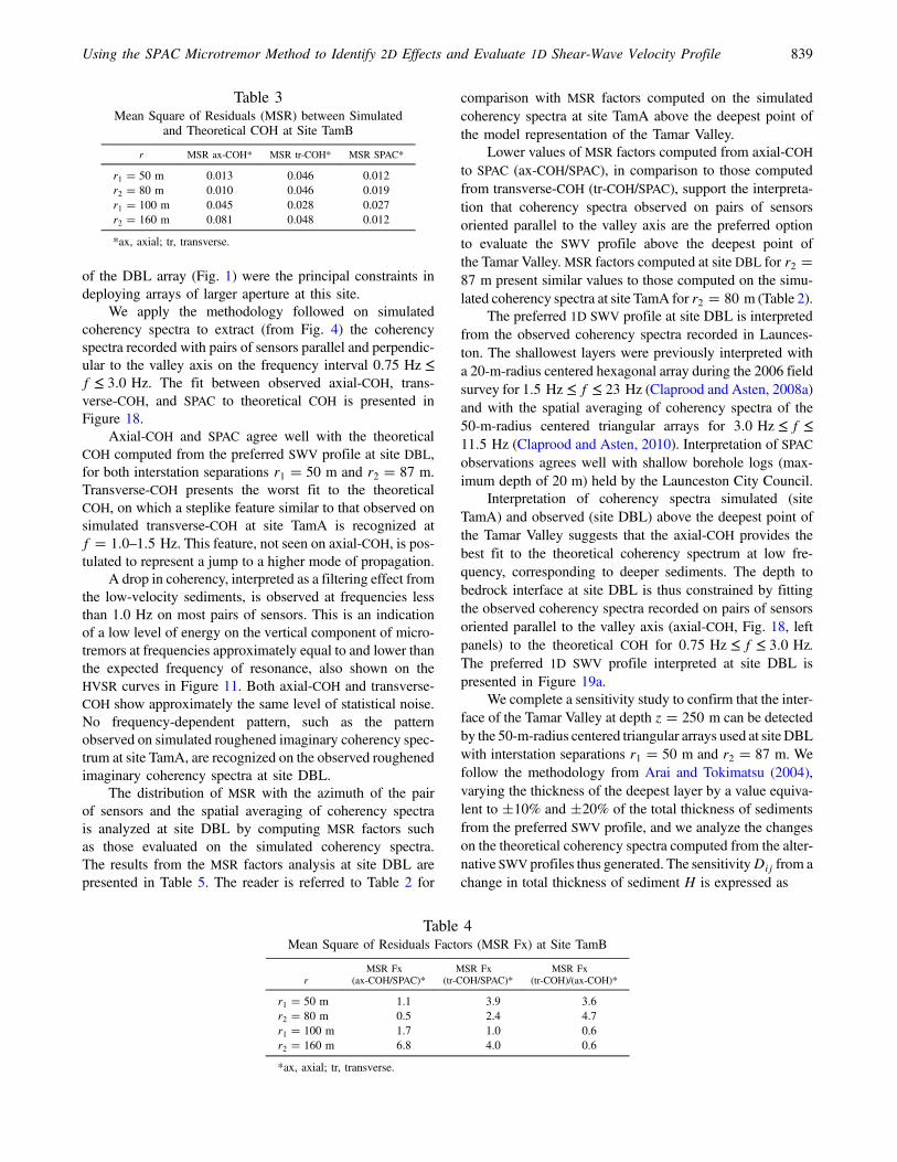
We use a fine grid of 901 × 361 × 43 cells and a coarsegrid of 101 × 41 × 96 cells to simulate the Tamar Valley,with a 10-m and 90-m spacing in the fine and coarse grids,respectively. Simulated SPAC arrays were positioned at twoseparate locations across the valley, with radii of 50 m and100 m. The sensors are positioned to form centered triangulararrays with orientation XA1 axial and XA2 transverse to thevalley axis to compare with SPAC observations recorded inLaunceston. The location of all 26 receivers is plotted inFigure 8.

An analytical expression of the valley interface is inputfor the numerical simulations of surface waves. As suggestedby the interpretation of gravity profiles from Leaman (1994),the valley geometry presents some asymmetry. The mostappropriate function to represent the Tamar Valley withrespect to horizontal distance x and depth z is the function

f�x; z� ��1� x

a

��1 � x

a

�1�ζ1�ζ �

��1� ζ��1 � ζ�1�ζ1�ζ

�z

H;

(6)

where a is the valley half-width, H is the maximum depth,and ζ the asymmetry coefficient (Paolucci, 1999). Figure 9ashows the simulated Tamar Valley bedrock interface, witha � 350 m, H � 250 m, and ζ � �0:28571. A layered

earth with depth to bedrock z � 25 m at the right of thevalley is interpreted from HVSR observations at Launceston(M. Claprood, M. Asten, and J. Kristek, unpublishedmanuscript).

Apart from lateral change in the bedrock interface, nolateral changes of velocity are considered in the overlayingsediments. This assumption was used to isolate and betterunderstand the effect of a change in the bedrock interfaceand is justified by preliminary SPAC and FK results and SPACobservations recorded at 10 sites in Launceston (Claproodand Asten, 2009a, 2009b). The 1D SWV profile used in thesimulations is presented in Figure 9b.

The 1D SWV profile presented in Figure 9b is an approx-imation of the SWV profile evaluated at site DBL fromprevious high-frequency coherency spectra analysis withconstraints from a gravity survey and HVSR observations(Claprood and Asten, 2008a, 2008b).

The shallow Quaternary sediments are modeled as a15-m layer of constant shear-wave velocity VS � 350 m=sto suppress numerical instabilities at the free surface, wherethe steep sediment bedrock interface reaches the free surface

0 1 2 3 4 5−0.5

0

0.5

1RGB, r1=50m

cohe

renc

y

frequency (Hz)

(a)

0 1 2 3 4 5−0.5

0

0.5

1RGB, r2=87m

frequency (Hz)

(b)

Figure 6. Observed coherency spectra at site RGB on all pairsof sensors and interstation separations of two centered triangulararrays for (a) r1 � 50 m and (b) r2 � 87 m. Same legend as forFigure 4.

−5000 −4000 −3000 −2000 −1000 0 1000 2000 3000 4000 5000−2000

−1000

0

1000

2000

distance X (m)

dist

ance

Y (

m)

Figure 7. Simulated sources used in the numerical simulationsof the Tamar Valley. Thick dotted line, the outline of the computa-tional model; thick dashed vertical lines, edges of the simulatedTamar Valley; crosses, locations of receivers (represented in moredetail in Figure 8).

−500 −250 0 250 500−300

−200

−100

0

100

200

300

location X (m)

loca

tion

Y (

m)

Figure 8. Location of simulated receivers across the modelrepresentation of the Tamar Valley. Arrays of radii 50 m and 100 mare presented for sites TamA�x � �100 m� andTamB�x � 100 m�.Solid vertical lines, edges of the valley (x � �350 m, x � 350 m);dashed vertical line, the axis of the valley at its deepest point(x � �100 m).

−600 −400 −200 0 200 400 600

0

100

200

TamA TamB(a)

location X (m)

dept

h (m

)

0 500 1000

0

100

200

(b)

VS (m/s)

Figure 9. (a) Bedrock interface of model representation ofTamar Valley (vertical extension of 2). Sites TamA and TamBare the surface locations of the SPAC arrays’ centers. Site TamAis located above the deepest point of the valley. Site TamB is located200 m from site TamA. The bedrock interface at site TamB is 156 mdeep, with a 38° slope. Dashed-dotted line is the geological inter-pretation of the bedrock interface from gravity profile 2 (Fig. 1b).Vertical dashed line in (a) is the location of SWV profile presentedin (b), at the deepest point of the valley.


at the grid boundary in the perfectly matched layer zone. Thisapproximation has negligible impact when analyzing thepropagation of surface waves generated by the valley. Wecalculate a negligible difference of 0.02 Hz when evaluatingthe expected frequency of resonance computed with theobserved SWV profile at site DBL and with the approximateSWV profile used in the simulations (thin 15-m layer withVS � 350 m=s). This suggests the SWV profile used in thenumerical simulations is an adequate approximation to repre-sent the SWV evaluated in the Tamar Valley.

The shear-wave velocity of Tertiary sediments is repre-sented by a linear function that varies from VS � 400 m=sat depth z � 15 m to VS � 700 m=s at depth z � 250 m.High quality factors were input for S-wave propagation(1000 ≤ QS ≤ 2000) and P-wave propagation (1500 ≤ QP ≤8000) to neglect the compressibility of sediments. Thisassumption is considered valid when dealing with low-amplitude waves such as microtremors.

Simulated SPAC

The outputs of the numerical simulations are the timeseries of the vertical and horizontal (X and Y components)ground velocity at all receivers. The vertical component timeseries of simulated microtremors are processed using thesame steps used to process SPAC observations in Launceston.Figure 10 presents the power spectra simulated at the centersensors X and sensors A from two 50 m radius and two100 m radius centered triangular arrays at site TamA.

The power spectra in Figure 10 show the restricted fre-quency interval input in the simulations. A rapid decrease inthe energy level is observed at all sensors for f > 3 Hz,which corresponds to the higher frequency limit input asinitial parameter. The simulated coherency spectra at differ-ent sites in the valley suggest the level of energy is sufficientto analyze SPAC curves for frequencies higher than 0.75 Hz.Sensors X and A1 (from both 50-m and 100-m radius arrays)present almost identical power spectra. This was expectedbecause all three sensors sample similar geology at the dee-pest point of the valley with a random source distribution.Small differences are observed between the power spectraof sensors A2 when moving away from the deepest point

of the valley at sensor X. The small increases in power spec-tra at approximately 1 Hz and 2 Hz are potentially inducedby varying geology under the sensor.

The energy level drops rapidly at lower frequencies,which is partly explained by the lower frequency limit inputin the simulations (0.4 Hz). We suggest the decrease in ver-tical microtremor energy at low frequency is further causedby the filtering effects of low-velocity sediments on verticalmotion. A previous study (Claprood and Asten, 2008b)estimated the SV mode of resonance at 1.18 Hz on HVSRobservations. Figure 11 presents the HVSR curves simulatedat the center sensors X at sites TamA and TamB and observedat center sensors X at sites DBL and RGB.

HVSR simulated (site TamA) and observed (DBL) abovethe deepest point of the valley present similar features andshape, further suggesting that the 2D model of the valleyis appropriate to represent the propagation of surface waveswithin the Tamar Valley.

Site TamA

The coherency spectra at site TamA, simulated from two50-m radius centered triangular arrays above the deepestpoint of the model representation of the Tamar Valley, arepresented in Figure 12. The pair of sensors XA1 is orientedaxially, and the pair of sensors XA2 is transverse to thevalley axis.

The results from two 100-m radius centered triangulararrays are presented in Figure 13 for improved resolutionat low frequencies and to better detect the impact of thevalley on simulated coherency spectra.

We observe from Figure 12 and Figure 13 that the simu-lated COH on all pairs of sensors present some variability forf > 1:0 Hz. Steplike features are observed on selected pairsof sensors at f � 1:0–1:5 Hz and f � 2:0–2:5 Hz. Suchfeatures associated with layered-earth sites have been inter-preted as evidence for jumps to higher modes of propagationon the coherency spectrum (Asten et al., 2004; Asten,2006b). We suggest these shifts to higher modes of propaga-tion on selected pairs of sensors are generated by 2D effectsfrom the Tamar Valley.

0.5 1 2 3 4 5 6

103

101

102

103

101

102

103

101

102

TamA, X

frequency (Hz)0.5 1 2 3 4 5 6

TamA, A1

frequency (Hz)0.5 1 2 3 4 5 6

TamA, A2

frequency (Hz)

Figure 10. Simulated vertical power spectra at site TamA. (Left) Power spectra from sensor X. (Center) Power spectra from array 1 atsensor A1. (Right) Power spectra from array 2 at sensor A2. Nomenclature of sensors and geometry of arrays 1 and 2 are defined in Figure 2.Solid spectra are for 50-m radius triangular arrays, dashed spectra are for 100-m radius triangular arrays. Sensor X is the same for all arrays.


We decompose the spatially averaged coherency spectrato analyze the behavior of simulated COH on selected pairs ofsensors. The decomposition of COH into pairs of sensors atvarious azimuths was found to give indications on the sourcedistribution of the microtremor wave field above a layeredearth (Claprood and Asten, 2010). We postulate that similarmethodology could assist in the detection of different modesof propagation in a valley environment, the valley polarizingthe propagation of seismic surface waves. We present thesimulated coherency spectrum at site TamA for pairs ofsensors oriented parallel (axial-COH, pairs of sensors XA1

and BC2 from Figure 12 and Figure 13) and perpendicular(transverse-COH, pairs of sensors XA2 and BC1 fromFigures 12 and 13) to the valley axis in Figure 14 andFigure 15. The theoretical coherency spectra of fundamentaland first higher modes, computed from the SWV profileshown in Figure 9b for interstation separations r1 �50–100 m and r2 � 80–160 m, are respectively drawn indashed and dashed-dotted lines in Figure 14 and Figure 15.

We observe from Figure 14 and Figure 15 that the simu-lated axial-COH and transverse-COH show different patternsin the frequency interval 0.75–2 Hz. The jump to higher

modes of propagation, already observed in Figure 12 andFigure 13, is better defined on simulated transverse-COHat f � 1:0 Hz � 1:5 Hz and is of increasing amplitude withincreasing interstation separation. This jump is not presenton simulated axial-COH, which more closely follows thetheoretical COH. The simulated transverse-COH presents thehighest level of roughened imaginary coherency spectrum inthe frequency interval 1:0 Hz ≤ f ≤ 2:0 Hz (black bars onFig. 14 and Fig. 15). This high statistical noise seems tobe azimuth dependent and is not observed on axial-COHand SPAC. The presence of high values of roughened imagin-ary coherency spectra could be induced by high-frequencynumerical instabilities generated by boundary effects of thefinite size grid used in the numerical simulations.

We summarize the MSR values computed between thetheoretical COH and simulated axial-COH, transverse-COH,and SPAC at site TamA on the frequency interval 0:75 Hz ≤f ≤ 3:0 Hz for the r1 � 50 m array and 0:75 Hz ≤ f ≤2:5 Hz for the r1 � 100 m array in Table 1. Different fre-quency intervals were selected to compare theoretical andsimulated COH in function on the array size in order to restrictthe analysis of coherency spectra computed with single pairsof sensors up the first minimum of the Bessel function, assuggested by Okada (2006) and Claprood and Asten (2010).

Lower values of the MSR on most axial-COH (r � 80 m,100 m, or 160 m), when compared to transverse-COHand SPAC on the selected frequency interval, suggest theuse of axial-COH alone is preferable to evaluate the 1DSWV profile from the microtremor time series simulated

101

101

100

101

100

100 101100101100101100

TamA

HV

SR

frequency (Hz)

TamB

frequency (Hz)

DBL

frequency (Hz)

RGB

frequency (Hz)

Figure 11. (Two left panels) Simulated HVSR at center sensors X at sites TamA and TamB. (Two right panels) Observed HVSR at centersensors X at sites DBL and RGB. Solid curves, total HVSR; dashed curves, axial component of HVSR; dashed-dotted curves, transversecomponent of HVSR. (X and Y axes are logarithmic). The color version of this figure is available only in the electronic edition.

0 1 2 3 4−0.5

0

0.5

1

−0.5

0

0.5

1TamA, r1=50m

cohe

renc

y

frequency (Hz)

(a)

0 1 2 3 4

TamA, r2=80m

frequency (Hz)

cohe

renc

y

(b)

Figure 12. Simulated coherency spectrum (COH) at site TamAon all pairs of sensors and interstation separations of two centeredtriangular arrays for (a) r1 � 50 m and (b) r2 � 80 m. Thick solidlines are spatially averaged coherency spectra (SPAC) on intersta-tion separations. Dashed lines are coherency spectra on pairs ofsensors parallel to the valley axis: XA1 on (a) and BC2 on (b).Dashed-dotted lines are coherency spectra on pairs of sensors trans-verse to the valley axis: XA2 on (a) and BC1 on (b). Thin solid linesare coherency spectra on all other pairs of sensors of the array. Pairsof sensors are named following the nomenclature presented inFigure 2. Straight line at bottom of each graph presents frequencyinterval where theoretical COH is fit to simulated COH. The colorversion of this figure is available only in the electronic edition.

0 1 2 3−0.5

0

0.5

1

−0.5

0

0.5

1TamA, r1=100m

cohe

renc

y

frequency (Hz)

(a)

0 1 2 3

TamA, r2=160m

frequency (Hz)

cohe

renc

y

(b)

Figure 13. Simulated COH at site TamA on all pairs of sensorsand interstation separations of two centered triangular arrays for(a) r1 � 100 m and (b) r2 � 160 m. Same legend as for Figure 12.The color version of this figure is available only in the electronicedition.


above the deepest point of a valley. It is an indication that thesimulated axial-COH presents the highest degree of similarityto the theoretical COH when considering the fundamentalmode of propagation of Rayleigh waves.

As suggested in Claprood and Asten (2010), we com-pute MSR factors to evaluate the azimuth dependency andthe impact of spatial averaging of simulated coherency spec-tra at site TamA. The MSR factors are computed as the ratio

0 2 4−0.5

0

0.5

1

−0.5

0

0.5

1

−0.5

0

0.5

1

−0.5

0

0.5

1

−0.5

0

0.5

1

−0.5

0

0.5

1

Axial − COH

Axial − COH

cohe

renc

y

MSR=0.024rms=0.098

0 2 4

Transv − COH

Transv − COH

MSR=0.020rms=0.112

0 2 4

r1=50m

MSR=0.012rms=0.014

0 2 4

cohe

renc

y

freq. (Hz)

MSR=0.021

rms=0.085

0 2 4

freq. (Hz)

MSR=0.049

rms=0.156

0 2 4

r2=80m

freq. (Hz)

MSR=0.022

rms=0.055

Figure 14. Best-fit coherency models for pairs of sensors and interstation separations (top row) r1 � 50 m and (bottom row) r2 � 80 mat site TamA. SPAC (right column) were computed from all pairs of sensors (n � 6) from two centered triangular arrays. Thick solid blackcurve, real component of simulated COH; gray solid curve, smoothed imaginary component of simulated COH; bars, roughened imaginarycomponent of simulated COH; dashed curve is theoretical COH, fundamental mode for preferred layered-earth model; dashed-dotted curve,theoretical COH, first higher mode. The straight line at the bottom of each graph presents the frequency interval where theoretical COH is fitto simulated COH. MSR, mean square of residuals; rmsIm, root mean square of the roughened imaginary component. The color version of thisfigure is available only in the electronic edition.

0 2 0 20 2−0.5

0

0.5

1

−0.5

0

0.5

1

−0.5

0

0.5

1

−0.5

0

0.5

1

−0.5

0

0.5

1

−0.5

0

0.5

1Axial − COH

Axial − COH

cohe

renc

y

MSR=0.024

rms=0.103

Transv − COH

Transv − COH

MSR=0.075

rms=0.143

r1=100m

MSR=0.043

rms=0.030

0 2

cohe

renc

y

freq. (Hz)

MSR=0.056

rms=0.121

0 2

freq. (Hz)

MSR=0.184

rms=0.173

0 2

r2=160m

freq. (Hz)

MSR=0.066

rms=0.069

Figure 15. Best-fit coherency models for pairs of sensors and interstation separations (top) r1 � 100 m and (bottom) r2 � 160 m at siteTamA. Same legend as for Figure 14. The color version of this figure is available only in the electronic edition.


of MSR values in two different situations. For example, wecompute an MSR factor of 0.6 between the simulated axial-COH and SPAC for r � 100 m at site TamA by dividing theMSR on axial-COH (0.024 from Table 1) by the MSR on SPAC(0.43 from Table 1). An MSR factor of 0.6 indicates the MSRcomputed on simulated axial-COH is smaller than the MSRcomputed on SPAC with r � 100 m at site TamA. Thissuggests that the axial-COH provides a better fit to the the-oretical coherency spectra to evaluate the 1D SWV profile.We use MSR factors to compare coherency spectra simulated(or observed) on pairs of sensors of different azimuths andspatially averaged coherency spectra.

Table 2 presents MSR factors computed at site TamA.The MSR factor referred to as ax-COH/SPAC is the ratiobetween the MSR on axial-COH and the MSR on SPAC. TheMSR factor referred to as tr-COH/SPAC is the ratio betweenthe MSR on transverse-COH and the MSR on SPAC, while theMSR factor referred to as tr-COH/ax-COH is the ratio betweenthe MSR on transverse-COH and the MSR on axial-COH.

The results fromTable 2 further indicate that axial-COH isthe preferred option to evaluate a 1D SWV profile above thedeepest point of the valley at site TamA for the selectedfrequency interval. The MSR factors ax-COH/SPAC are loweror equal to 1:0x for all interstation separations exceptr � 50 m. In Figure 14 (top left panel), the simulated axial-COH closely follows the theoretical COH for r � 50 m,and departure from the theoretical COH is observed forfrequencies greater than 2 Hz.

Site TamB

Simulated coherency spectra are recorded at site TamB,modeling a location over the sloping flank of the TamarValley. We present the simulated COH for pairs of sensorsoriented parallel (axial-COH) and perpendicular (transverse-COH) to the valley axis in Figure 16 and Figure 17.

We observe that the simulated coherency spectra presenta different pattern at site TamB compared to site TamA. Thejump to a higher mode of propagation is not observed onpairs of sensors at f � 1:0 Hz–1:5 Hz at site TamB. HigherMSR on axial-COH and transverse-COH in comparison withSPAC on larger interstation separations, which are more sen-sitive to deeper material, suggest the conventional azimuthalaveraging of coherency spectra is preferable in evaluatingthe 1D SWV profile down to the basement at site TamB.Localized high values of statistical noise (high rmsIm) is alsoobserved at most pairs of sensors on the simulated coherencyspectra.

MSR computed for axial-COH, transverse-COH, andSPAC are summarized in Table 3. As completed for site TamA,we present the MSR factors computed at site TamB in Table 4.

High MSR factors on both axial-COH and transverse-COH relative to SPAC for most interstation separations furtherstrengthen the evidence that the azimuthal averaging ofcoherency spectra is needed to evaluate the 1D SWV profileat site TamB for the selected frequency interval. The highMSR factors computed from axial-COH to SPAC at site TamBfor larger interstation separations, compared to those evalu-ated at site TamA (Table 2), is evidence that the varyinggeological conditions impact the two locations differently.

The analysis of the coherency spectra simulated at sitesTamA and TamB in the model representation of the TamarValley suggests the decomposition of the spatially averagedcoherency spectrum into components oriented parallel(axial-COH) and perpendicular (transverse-COH) to the valleyaxis is an effective method for the recognition of 2D effectsinduced by the deep and narrow Tamar Valley. This effectis seen as a jump to higher modes of propagation at f �1:0 Hz–1:5 Hz on the transverse-COH at site TamA, locatedabove the deepest point of the model representation of thevalley. Possible 2D effects could be detected at higher fre-quency (jump to higher modes at f � 2:0 Hz–2:5 Hz at siteTamA) butwould be difficult to isolate on observed coherencyspectra at sites DBL and RGB due to the increased variabilityof the observed coherency spectra at higher frequency.

The results from the numerical simulations suggest thatthe coherency spectra computed on pairs of sensors orientedparallel to the valley axis (axial-COH) can provide a reliableestimation of 1D SWV structure above the deepest point of avalley because its fit to the theoretical coherency spectrumpresents lower MSR than the transverse-COH or the spatiallyaveraged coherency spectrum.

Table 1Mean Square of Residuals (MSR) between Simulated

and Theoretical COH at Site TamA

r MSR ax-COH* MSR tr-COH* MSR SPAC

r1 � 50 m 0.024 0.020 0.012r2 � 80 m 0.021 0.049 0.022r1 � 100 m 0.024 0.075 0.043r2 � 160 m 0.056 0.184 0.066

*ax, axial; tr, transverse.

Table 2Mean Square of Residuals Factors (MSR Fx) at Site TamA

rMSR Fx

(ax-COH/SPAC)*MSR Fx

(tr-COH/SPAC)*MSR Fx

(tr-COH)/(ax-COH)*

r1 � 50 m 2.0 1.7 0.8r2 � 80 m 1.0 2.2 2.3r1 � 100 m 0.6 1.7 3.1r2 � 160 m 0.9 2.8 3.3



Observed SPAC

Similar methodology was applied at sites DBL andRGB in Launceston to validate the results obtained fromthe numerical simulations and to detect the effects of rapidchanges in geology across the Tamar Valley. Site DBL is as-sumed to be located above the deepest point of the TamarValley in order to compare with site TamA, and site RGB

is located in the east flank of the valley at similar positionto that of site TamB.

Site DBL

Coherency spectra were recorded at site DBL with two50-m-radius centered triangular arrays. The heavy traffic onWellington Street and the steep hill on Frankland Street west

0 2 4−0.5

0

0.5

1

−0.5

0

0.5

1

−0.5

0

0.5

1

−0.5

0

0.5

1

−0.5

0

0.5

1

−0.5

0

0.5

1

Axial − COH

Axial − COH

cohe

renc

y

MSR=0.013rms=0.082

0 2 4

Transv − COH

Transv − COH

MSR=0.046rms=0.083

0 2 4

r1=50m

MSR=0.012rms=0.020

0 2 4

cohe

renc

y

freq. (Hz)

MSR=0.010

rms=0.127

0 2 4

freq. (Hz)

MSR=0.046

rms=0.098

0 2 4

r2=80m

freq. (Hz)

MSR=0.019

rms=0.052

Figure 16. Best-fit coherency models from pairs of sensors and interstation separations (top) r1 � 50 m and (bottom) r2 � 80 m at siteTamB. Same legend as for Figure 14. The color version of this figure is available only in the electronic edition.

0 2−0.5

0

0.5

1

−0.5

0

0.5

1

−0.5

0

0.5

1

−0.5

0

0.5

1

−0.5

0

0.5

1

−0.5

0

0.5

1

Axial − COH

cohe

renc

y

MSR=0.045

rms=0.061

0 2

Transv − COH

Axial − COH Transv − COH

MSR=0.028

rms=0.112

0 2

r1=100m

MSR=0.027

rms=0.018

0 2

cohe

renc

y

freq. (Hz)

MSR=0.081

rms=0.155

0 2

freq. (Hz)

MSR=0.048

rms=0.109

0 2

r2=160m

freq. (Hz)

MSR=0.012

rms=0.095

Figure 17. Best-fit coherency models from pairs of sensors and interstation separations (top) r1 � 100 m and (bottom) r2 � 160 m atsite TamB. Same legend as for Figure 14. The color version of this figure is available only in the electronic edition.


of the DBL array (Fig. 1) were the principal constraints indeploying arrays of larger aperture at this site.

We apply the methodology followed on simulatedcoherency spectra to extract (from Fig. 4) the coherencyspectra recorded with pairs of sensors parallel and perpendic-ular to the valley axis on the frequency interval 0:75 Hz ≤f ≤ 3:0 Hz. The fit between observed axial-COH, trans-verse-COH, and SPAC to theoretical COH is presented inFigure 18.

Axial-COH and SPAC agree well with the theoreticalCOH computed from the preferred SWV profile at site DBL,for both interstation separations r1 � 50 m and r2 � 87 m.Transverse-COH presents the worst fit to the theoreticalCOH, on which a steplike feature similar to that observed onsimulated transverse-COH at site TamA is recognized atf � 1:0–1:5 Hz. This feature, not seen on axial-COH, is pos-tulated to represent a jump to a higher mode of propagation.

A drop in coherency, interpreted as a filtering effect fromthe low-velocity sediments, is observed at frequencies lessthan 1.0 Hz on most pairs of sensors. This is an indicationof a low level of energy on the vertical component of micro-tremors at frequencies approximately equal to and lower thanthe expected frequency of resonance, also shown on theHVSR curves in Figure 11. Both axial-COH and transverse-COH show approximately the same level of statistical noise.No frequency-dependent pattern, such as the patternobserved on simulated roughened imaginary coherency spec-trum at site TamA, are recognized on the observed roughenedimaginary coherency spectra at site DBL.

The distribution of MSR with the azimuth of the pairof sensors and the spatial averaging of coherency spectrais analyzed at site DBL by computing MSR factors suchas those evaluated on the simulated coherency spectra.The results from the MSR factors analysis at site DBL arepresented in Table 5. The reader is referred to Table 2 for

comparison with MSR factors computed on the simulatedcoherency spectra at site TamA above the deepest point ofthe model representation of the Tamar Valley.

Lower values of MSR factors computed from axial-COHto SPAC (ax-COH/SPAC), in comparison to those computedfrom transverse-COH (tr-COH/SPAC), support the interpreta-tion that coherency spectra observed on pairs of sensorsoriented parallel to the valley axis are the preferred optionto evaluate the SWV profile above the deepest point ofthe Tamar Valley. MSR factors computed at site DBL for r2 �87 m present similar values to those computed on the simu-lated coherency spectra at site TamA for r2 � 80 m (Table 2).

The preferred 1D SWV profile at site DBL is interpretedfrom the observed coherency spectra recorded in Launces-ton. The shallowest layers were previously interpreted witha 20-m-radius centered hexagonal array during the 2006 fieldsurvey for 1:5 Hz ≤ f ≤ 23 Hz (Claprood and Asten, 2008a)and with the spatial averaging of coherency spectra of the50-m-radius centered triangular arrays for 3:0 Hz ≤ f ≤11:5 Hz (Claprood and Asten, 2010). Interpretation of SPACobservations agrees well with shallow borehole logs (max-imum depth of 20 m) held by the Launceston City Council.

Interpretation of coherency spectra simulated (siteTamA) and observed (site DBL) above the deepest point ofthe Tamar Valley suggests that the axial-COH provides thebest fit to the theoretical coherency spectrum at low fre-quency, corresponding to deeper sediments. The depth tobedrock interface at site DBL is thus constrained by fittingthe observed coherency spectra recorded on pairs of sensorsoriented parallel to the valley axis (axial-COH, Fig. 18, leftpanels) to the theoretical COH for 0:75 Hz ≤ f ≤ 3:0 Hz.The preferred 1D SWV profile interpreted at site DBL ispresented in Figure 19a.

We complete a sensitivity study to confirm that the inter-face of the Tamar Valley at depth z � 250 m can be detectedby the 50-m-radius centered triangular arrays used at site DBLwith interstation separations r1 � 50 m and r2 � 87 m. Wefollow the methodology from Arai and Tokimatsu (2004),varying the thickness of the deepest layer by a value equiva-lent to �10% and �20% of the total thickness of sedimentsfrom the preferred SWV profile, and we analyze the changeson the theoretical coherency spectra computed from the alter-native SWV profiles thus generated. The sensitivityDij from achange in total thickness of sediment H is expressed as

Table 3Mean Square of Residuals (MSR) between Simulated

and Theoretical COH at Site TamB

r MSR ax-COH* MSR tr-COH* MSR SPAC*

r1 � 50 m 0.013 0.046 0.012r2 � 80 m 0.010 0.046 0.019r1 � 100 m 0.045 0.028 0.027r2 � 160 m 0.081 0.048 0.012


Table 4Mean Square of Residuals Factors (MSR Fx) at Site TamB

rMSR Fx



(tr-COH)/(ax-COH)*

r1 � 50 m 1.1 3.9 3.6r2 � 80 m 0.5 2.4 4.7r1 � 100 m 1.7 1.0 0.6r2 � 160 m 6.8 4.0 0.6



DHi �f� �

�� H

J0�f�×∂J0�f�∂H

��H�Hi

; (7)

where J0 is the theoretical coherency spectrum, and i corre-sponds to the change in the parameter evaluated (H � 10%

and H � 20%). The results from the sensitivity study arepresented in Figure 19b.

While the absolute values of sensitivity are not high, thevariation of sensitivity (most significant on interstation sep-aration r2, Fig. 19b) at 1:0 Hz ≤ f ≤ 2:0 Hz, with a changein total thickness of 10% or 20%, confirms the capabilities ofobserved COH at site DBL to locate the bedrock interface atdepth z � 250 m. The frequency for which the jump to ahigher mode of propagation was detected on transverse-COH (Fig. 18) is included in this frequency interval. It furtherstrengthens the idea that the differences observed in thebehavior of axial-COH and transverse-COH can be inducedby the sensitivity of each component to the different modesof propagation that develop in the Tamar Valley. The infinitepeak observed at f≃ 2:0 Hz on r2 (Fig. 19b, right panel) isinduced by the zero crossing of the Bessel function at thatfrequency and is a mathematical artifact of equation (7).

We evaluate the MSR between the observed coherencyspectra on axial-COH, transverse-COH, and SPAC and fromthe theoretical COH computed from the preferred and alter-native SWV profiles obtained from the sensitivity study. Wealso evaluate MSR factors between the MSR computed onalternative SWV profiles and the MSR computed on the pre-ferred SWV profile on axial-COH, transverse-COH, andSPAC. Table 6 presents a summary of MSR and MSR factorscomputed during the sensitivity study at site DBL.

While the variations inMSR are quite small, clear tenden-cies can be observed from Table 6. As expected, the intersta-tion separation r2 is more sensitive to a change in the totalthickness of sediments. While the MSR computed on SPACstay constant with a variation in thickness, MSR values onaxial-COH and transverse-COH have opposite reactions.Shallowing the bedrock interface (H � 20%, H � 10%)worsens the fit obtained with axial-COH, while it improvesthe fit obtained with transverse-COH. Deepening the interface(H � 20%, H � 10%) seems to improve the fit obtainedwith axial-COH, while it has no effect on the fit obtained withtransverse-COH. We suggest the lower MSR on axial-COHwith a deeper bedrock interface is an artifact induced by

0 2 4−0.5

0

0.5

1

−0.5

0

0.5

1

−0.5

0

0.5

1

−0.5

0

0.5

1

−0.5

0

0.5

1

−0.5

0

0.5

1

Axial − COH

Axial − COH

cohe

renc

y

MSR=0.008rms=0.026

0 2 4

Transv − COH

Transv − COH

MSR=0.015rms=0.017

0 2 4

r1=50m

MSR=0.005rms=0.007

0 2 4

cohe

renc

y

freq. (Hz)

MSR=0.014

rms=0.024

0 2 4

freq. (Hz)

MSR=0.028

rms=0.026

0 2 4

r2=87m

freq. (Hz)

MSR=0.015

rms=0.010

Figure 18. Best-fit coherency models from pairs of sensors and interstation separations (top) r1 � 50 m and (bottom) r2 � 87 m at siteDBL. Same legend as for Figure 14. The color version of this figure is available only in the electronic edition.

Table 5Mean Square of Residuals Factors (MSR Fx) at Site DBL

rMSR Fx



(tr-COH)/(ax-COH)*

r1 � 50 m 1.6 3.0 1.9r2 � 87 m 0.9 1.9 2.0



the observed drop in coherency spectra for frequencies lowerthan the frequency of resonance. The opposite reaction to achange in sediments thickness observed on axial-COH andtransverse-COH further supports the idea that the two compo-nents record different information from themicrotremor wavefield propagating in the Tamar Valley.

Site RGB

Coherency spectra were recorded at site RGB with two50-m-radius centered triangular arrays. Figure 20 shows theobserved coherency spectra at site RGB, recorded with pairsof sensors parallel (axial-COH) and perpendicular (trans-verse-COH) to the valley axis and the spatially averagedcoherency spectra for interstation separations r1 � 50 mand r2 � 87 m.

Observed coherency spectra at site RGB are interpretedfor 0:5 Hz ≤ f ≤ 4:25 Hz. All observed coherency spectra(axial-COH, transverse-COH, SPAC) agree well with thetheoretical COH computed from the preferred SWV profile atsite RGB. Observed COHs from all azimuths present a dropin coherency at approximately 1.0 Hz, effects which mightbe induced by the filtering effects of low-velocity sediments

at the frequency of resonance, evaluated at f � 1:31 Hzfrom HVSR (Fig. 11).

A jump to a higher mode of propagation is observed ontransverse-COH at f ≥ 2:0 Hz, while it is only lightly detect-able on r2 on axial-COH. The decomposition of SPAC intopairs of sensors, presented in Claprood and Asten (2010), hassuggested the presence of limited azimuth distribution ofmicrotremor energy at site RGB, which might mask possible2D effects induced by the Tamar Valley at these frequencies.We suggest this jump to higher mode, associated with highlycyclic behavior of the smoothed imaginary coherency spec-trum (gray curve, Fig. 20) is induced by limited azimuthsampling in the microtremor wave field.

An MSR analysis similar to that conducted at site DBL ispresented in Table 7 to better analyze the azimuth samplingof observed coherency spectra at site RGB.

High MSR factors between the MSR computed on axial-COH and transverse-COH with respect to SPAC suggest theimportance of spatial averaging the observed coherencyspectra at site RGB to obtain a reliable evaluation of the 1DSWV profile. MSR factors ax-COH/SPAC and tr-COH/SPACpresent similar values for both interstation separations. Thisfurther strengthens the hypothesis that neither axial-COH nortranverse-COH should be used alone to evaluate the 1D SWVprofile at site RGB. This is a significant difference whencompared with site DBL, where the axial-COH was the pre-ferred option to evaluate the SWV profile.

This difference is explained by the location of both siteswithin the valley; site RGB is located above the gentle slopeon the eastern flank of the Tamar Valley, which can beestimated as a layered earth, while site DBL is assumedto be located above the deepest point of the Tamar Valley,where a 2D resonance is expected to develop. The HVSRcurves presented in Figure 11 also suggest that the approx-imation of a 1D layered earth is valid at site RGB, where bothaxial and transverse components of HVSR show a peak at thesame frequency.

Similar to completed at site DBL, a sensitivity study wascompleted to analyze the possibility of detecting the bedrock

0 500 1000

0

50

100

150

200

250

300

(a) (b)Site DBL

VS (m/s)

dept

h (m

)

0 1 2 3

0

0.5

1

1.5

2

r1=50m

Sen

sitiv

ity o

f J0(

kr)

frequency (Hz)

H − 20%H − 10%H + 10%H + 20%

0 1 2 3

0

0.5

1

1.5

2

r2=87m

frequency (Hz)

H − 20%H − 10%H + 10%H + 20%

Figure 19. (a) Preferred 1D SWV profile interpreted at siteDBL (thick black line). Thin gray and black lines are alternativeSWV profiles used in the sensitivity study. (b) Sensitivity studyon theoretical COH by varying the total sediment thickness by H �10% and H � 20%. Straight line at bottom of graph presents thevalid frequency interval at site DBL.

Table 6Mean Square of Residuals and MSR Factors* between Axial-COH, Transverse-COH, and SPAC Recorded

at Site DBL and Theoretical COH Computed from Preferred and Alternative SWV Profiles

ax-COH† tr-COH† SPAC ax-COH† tr-COH† SPAC

r1 � 50 m r1 � 50 m r1 � 50 m r2 � 87 m r2 � 87 m r2 � 87 m

MSR Computed from Preferred SWV ProfileH‡ 0.008 0.015 0.005 0.014 0.028 0.015

MSR (and MSR Factors*) Computed from Alternative SWV ProfilesH � 20%‡ 0:009�1:1x� 0:014�0:9x� 0:005�1:0x� 0:018�1:3x� 0:025�0:9x� 0:015�1:0x�H � 10%‡ 0:008�1:0x� 0:015�1:0x� 0:005�1:0x� 0:015�1:1x� 0:027�1:0x� 0:015�1:0x�H � 10%‡ 0:007�0:8x� 0:015�1:0x� 0:005�1:0x� 0:012�0:9x� 0:028�1:0x� 0:015�1:0x�H � 20%‡ 0:007�0:9x� 0:015�1:0x� 0:004�0:8x� 0:011�0:8x� 0:028�1:0x� 0:014�0:9x�

*MSR factors (in parentheses) are computed as the ratio of MSR from alternative SWV profiles to MSR from preferred SWVprofile.

†ax, axial; tr, transverse.‡H, total thickness of sediment.


interface on the valid frequency interval used at site RGB.The results are presented in Figure 21.

The sensitivity study shows that there is little sensitivityto changes in the bedrock interface at site RGB; this is trueeven if the depth to bedrock interface is interpreted as muchshallower than at site DBL.We believe the shallow sedimentsof very low velocity that were encountered at site RGB have amasking effect, limiting the resolution at greater depth.

Residuals Analysis

An analysis of residuals between the simulated andobserved coherency spectra from all interstation separationsof all arrays and the theoretical coherency spectra J0 com-puted from the preferred 1D SWV helps us to summarizethe results obtained at Launceston. Figure 22 presents thefrequency distribution of residuals computed at simulatedsites TamA and TamB and observed sites DBL and RGB.The residuals are computed as the difference between eachcomponent of the simulated or observed coherency spectra(axial-COH, transverse-COH, SPAC) and the theoreticalcoherency spectrum on the valid frequency interval.

Figure 22 better represents the differences between allcomponents of simulated or observed coherency spectraand the theoretical coherency spectra (Bessel function J0).The residuals computed from the transverse-COH (dashed-dotted curves, Fig. 22a–d) show a peak-and-trough featureat f � 1:0–1:5 Hz at site TamA. The amplitude of the peaksand the troughs on transverse-COH residuals is increasingwith larger interstation separation. This feature is notobserved on axial-COH (dashed curves, Fig. 22a–d). The re-siduals computed from SPAC present a behavior betweenthose of axial-COH and transverse-COH. No such trend canbe observed at site TamB (Fig. 22e–h), where the residualsbehave more randomly regardless of the component fromwhich they are computed.

The peak and trough feature on the residuals oftransverse-COH is also observed at site DBL, for r � 87 m,while it is not present on the other components (axial-COHand SPAC in Fig. 22i,j). Residuals at site RGB behave in asimilar way, regardless of the component used to computethem (Fig. 22k,l). At all simulated and observed arrays,we clearly observe more variability in the residuals for higherfrequencies (f ≥ 2:0 Hz) for axial-COH and transverse-COH,

0 2 4−0.5

0

0.5

1

−0.5

0

0.5

1

−0.5

0

0.5

1

−0.5

0

0.5

1

−0.5

0

0.5

1

−0.5

0

0.5

1

Axial − COH

cohe

renc

y

MSR=0.015

rms=0.022

0 2 4

Transv − COH

Axial − COH Transv − COH

MSR=0.010

rms=0.031

0 2 4

r1=50m

MSR=0.002

rms=0.009

0 2 4

cohe

renc

y

freq. (Hz)

MSR=0.035

rms=0.043

0 2 4

freq. (Hz)

MSR=0.038

rms=0.025

0 2 4

r2=87m

freq. (Hz)

MSR=0.008

rms=0.014

Figure 20. Best-fit coherency models from pairs of sensors and interstation separations (top) r1 � 50 m and (bottom) r2 � 87 m at siteRGB. Same legend as for Figure 14. The color version of this figure is available only in the electronic edition.

Table 7Mean Square of Residuals Factors (MSR Fx) at Site RGB

rMSR Fx



(tr-COH)/(ax-COH)*

r1 � 50 m 7.5 5.0 0.7r2 � 87 m 4.4 4.8 1.1



while the residuals computed from SPAC show morestability.

1D SWV Profiles

The preferred SWV profiles interpreted at sites DBL andRGB are presented in Figure 23a. Figure 23b shows theshear-wave slowness profiles to better represent the varia-tions in velocity in the low-velocity layers, as suggested byBoore and Asten (2008).

Significant differences are observed between thepreferred SWV profiles interpreted at sites DBL and RGB.The shallow layers (z < 25 m) at site RGB have significantlylower velocity (greater slowness; Fig. 23b) than the shallowsediments at site DBL. This could be explained by the proxi-mity of the site RGB to the Tamar River (Fig. 1a), where theshallow sediments are known to possess very little cohesion,thus lower shear-wave velocity. Sediments with velocityvarying between 400 m=s and 700 m=s are interpreted assands and clays from the Tertiary period, filling most ofthe Tamar Valley. Tertiary sediments are significantly thickerat site DBL; the interface with the Jurassic dolerite bedrock isinterpreted at approximately z � 250 m at site DBL and z �100 m at site RGB. Because of the poor sensitivity of thearrays at site RGB, the bedrock interface at this location isbest constrained by HVSR observations (J. Kristek, P. Moczo,and M. Kristekova, unpublished manuscript).

Interpretation of Results

As described in Bard and Bouchon (1985), and lateridentified by Steimen et al. (2003), Frischknecht and Wagner(2004), Roten et al. (2006), and Lenti et al. (2009), differentmodes of resonance develop in a valley environment. Inshallow valleys, Bard and Bouchon’s model states that sur-face waves are generated from the edges of the valley andpropagate back and forth within the sediments, inducing a1D pattern of resonance. In deep and narrow valleys, differentmodes of resonance develop (SH, SV, P), with their

0 1 2 3−0.5

0

0.5

−0.5

0

0.5

−0.5

0

0.5

−0.5

0

0.5

−0.5

0

0.5

−0.5

0

0.5

−0.5

0

0.5

−0.5

0

0.5

−0.5

0

0.5

−0.5

0

0.5

−0.5

0

0.5

−0.5

0

0.5

(a) TamA, r1=50m

CO

H −

J0

CO

H −

J0

CO

H −

J0

CO

H −

J0

CO

H −

J0

CO

H −

J0

0 1 2 3

(b) TamA, r2=80m

0 1 2 3

(c) TamA, r1=100m

0 1 2 3

(d) TamA, r2=160m

0 1 2 3

(e) TamB, r1=50m

0 1 2 3

(f) TamB, r2=80m

0 1 2 3

(g) TamB, r1=100m

0 1 2 3

(h) TamB, r2=160m

0 1 2 3

(i) DBL, r1=50m

0 1 2 3

(j) DBL, r2=87m

0 1 2 3

(k) RGB, r1=50m

freq. (Hz)0 1 2 3

(l) RGB, r2=87m

freq. (Hz)

Figure 22. Distribution of residuals with frequency for allinterstation separations at simulated arrays (a,b,c,d) TamA and(e,f,g,h) TamB and at observed arrays (i,j) DBL and (k,l) RGB.Solid curves, simulated or observed SPAC minus theoretical Besselfunction J0; dashed curves, simulated or observed axial-COH minusJ0; dashed-dotted curves, simulated or observed transverse-COH minus J0. The color version of this figure is available onlyin the electronic edition.

0 500 1000

0

50

100

150

200

250

(a)

VS (m/s )

dept

h (m

)

0 2 4 6

0

50

100

150

200

250

(b)

slow. (ms/m)

dept

h (m

)

Figure 23. Preferred (a) 1D SWV-to-depth profiles and (b) 1Dslowness-to-depth profiles at sites DBL (solid lines) and RGB(dashed lines).

0 1 2 3 4

0

0.5

1

1.5

2

r1=50m

Sen

sitiv

ity o

f J0(

kr)

frequency (Hz)

(b)H − 20%H − 10%H + 10%H + 20%

0 1 2 3 4

0

0.5

1

1.5

2

r2=87m

frequency (Hz)

H − 20%H − 10%H + 10%H + 20%

0 500 1000

0

50

100

150

200

250

300

Site RGB

VS (m/s)

dept

h (m

)(a)

Figure 21. (a) Preferred 1D SWV profile interpreted at siteRGB (thick black line). Thin gray and black lines are alternativeSWV profiles used in the sensitivity study. (b) Sensitivity studyon theoretical COH by varying the total sediment thickness by H �10% and H � 20%. Straight line at bottom of graph presents thevalid frequency interval at site RGB.


own frequencies of resonance and components of motion.The Bard and Bouchon (1985) model states that a 2D patternof resonance develops in valleys with a shape ratio (referredto as the ratio of maximum depthH to width at half-depth w)greater than a critical shape ratio. The model recognizes thedevelopment of a 2D pattern of resonance by the generationof standing waves from the bottom of the valley and indicatesthat edge-generated surface waves can also be detected.

As evaluated in Claprood and Asten (2008b), a 2D SVfrequency of resonance is identified in the Tamar Valley(shape ratio of 0.59) at f � 1:18 Hz at site DBL. The shaperatio is computed as the ratio of the maximum sedimentsthickness (H � 250 m) to the width at half-depth (w �421 m) evaluated from the model representation of the valley(Fig. 9a). The velocity contrast is computed for a doleritebedrock shear-wave velocity estimated at 1800 m=s andsediment shear-wave velocity of 350–700 m=s, evaluatedfrom the SWV profile used in the simulations at the deepestpoint of the valley at site TamA (Fig. 9b).

The Bard and Bouchon (1985) model indicates that theexcitation of SV waves induces mostly Rayleigh waves offirst higher mode of propagation in shallow valleys. Rayleighwaves of first higher mode have a greater velocity, whichapproximately equals the P-wave velocity of sediments atthe frequency of resonance of a layered earth. These edge-generated waves propagate from one edge of the valley to theother in a direction perpendicular to the valley axis.

We suggest the observed coherency spectra recorded bythe pairs of sensors oriented transverse to the valley axis candetect the transverse motion of propagation of these edge-generated waves. This is suggested by the jump to highermode of propagation recognized on simulated (site TamA)and observed (site DBL) transverse-COH recorded above thedeepest point of the valley; this jump occurs at a frequencyapproximately equal to the SV frequency of resonance of theTamar Valley.

From the absence of a jump on the axial-COH curves, wesuggest the axial-COH is free of the higher mode of surfacewave propagation at f � fSVfund and can be used with reliabil-ity to evaluate a 1D SWV profile in valley environment, asdemonstrated by numerical simulations and SPAC observa-tions in the Tamar Valley.

Conclusion

Numerical simulations of the propagation of seismicwaves from ambient seismic sources (microtremors) in avalley environment and microtremor observations in theTamar Valley in Launceston (Tasmania, Australia) were usedto assess the potential usefulness of the SPACmethod in study-ing complex geology. The recording of coherency spectra onpairs of sensors oriented parallel (axial-COH) and perpendic-ular (transverse-COH) to the valley axis optimizes the capabil-ity of the SPACmethod to detect the existence of the valley, toidentify its SV mode of resonance, and, most importantly, toevaluate a 1D SWV profile above the deepest point of the

valley. The use of axial-COH alone is recommended onlywhen microtremor sources are recorded for sufficient longtime and are distributed over a wide range of azimuth, bothassumptions being necessary for a meaningful SPAC estimateusing single pair of sensors.

We observe that coherency spectra recorded above thedeepest point of the valley with pairs of sensors orientedperpendicular to the valley axis can detect high-velocityedge-generated surface waves at the SV frequency of reso-nance. This was recognized on simulated transverse-COHat site TamA and on observed transverse-COH at site DBLabove the deepest point of the TamarValley, as a jump to fastervelocity on coherency spectra at a frequency approaching theSV fundamental frequency of resonance.

We suggest that the coherency spectra of the verticalcomponent computed on pairs of sensors oriented parallelto the valley axis (axial-COH) is not affected by the propaga-tion of these edge-generated waves of higher velocity.No jump to higher mode of propagation was detected onsimulated or observed axial-COH, which closely follows thetheoretical coherency spectra computed from the preferredSWV profile.

Lower mean square of residuals between simulated andtheoretical coherency spectra on axial-COH, when comparedto MSR values on transverse-COH and SPAC, suggest that thecoherency spectra recorded on pairs of sensors orientedparallel to the valley axis are the preferred option to evaluatea 1D SWV profile above the deepest point of the valley.

This is observed on simulated coherency spectra at siteTamA from 50-m-radius and 100-m-radius centered triangu-lar arrays. Observed coherency spectra recorded at site DBLabove the deepest point of the valley suggest similar conclu-sions. MSR values computed between observed axial-COH atsite DBL and theoretical coherency spectra are lower orapproximately equal to MSR values computed for SPACand are significantly lower than MSR values computed ontransverse-COH. This suggests that the observed coherencyspectra recorded with pairs of sensors parallel to a valley axisprovide a reliable evaluation of the 1D SWV profile at siteslocated above the deepest point of a deep and narrow valley,such as demonstrated above the Tamar Valley in Launceston.

Simulated coherency spectra in the sloping flank of thevalley (site TamB) suggest that no effect of the higher veloc-ity propagating surface waves is observed at this location. Wesuggest the gently dipping interface of this side of the valleydissipates the propagation of edge-generated higher modewaves. Numerical simulations suggest it is preferable to usethe spatially averaged coherency spectrum to evaluate the 1DSWV profile at site TamB, at which site the assumption of alayered earth holds true for microtremor studies. The coher-ency spectra observed at site RGB in the flank of the TamarValley prorogate the interpretation completed on simulatedcoherency spectra at site TamB. The presence of 1D and2D modes of resonance within the same valley has also beenobserved by Lenti et al. (2009).


These initial results demonstrate the capability of SPACobservations to detect the existence of a 2D structure, and tointerpret 1D SWV profiles in the environment of a deep andnarrow valley such as the Tamar Valley with a shape ratio of0.59. SPAC observations are combined with HVSR microtre-mor observations recorded in Launceston to complete the siteresonance study of the Tamar Valley (J. Kristek, P. Moczo,and M. Kristekova, unpublished manuscript). Additionalfield observations with larger arrays would help gain resolu-tion at depth, although at this site the deployment of largerarrays was restricted by the street layout. The use of three-component SPAC observations should provide additional in-formation, in particular by permitting the detection of the SHmode of resonance, which develops in valley environments.

Data and Resources

All data used in this paper came from published sourceslisted in the references. Information on the geology of Laun-ceston is available from unpublished maps from MineralResources Tasmania, borehole logs held by Launceston CityCouncil, and a gravity survey completed by Leaman (1994).

Acknowledgments

Maxime Claprood is supported by a Monash Graduate Scholarship, anInternational Postgraduate Research Scholarship, and a Québec’s Funds forNature and Technology Scholarship. Seismometers used in this project wereloaned to Monash University by the Australian National Seismic ImagingResource (ANSIR). We are grateful to the City Council of Launcestonfor their assistance during field surveys. Geological maps of Launcestonwere provided by Mineral Resources Tasmania. We would like to recognizethe help of Janett Steiner for her assistance during the field survey. We wishto thank associate editor Stefano Parolai and two anonymous reviewers,whose comments helped improve the manuscript.

References

Aki, K. (1957). Space and time spectra of stationary stochastic waves,with special reference to microtremors, Bull. Earthq. Res. Inst. 35,415–456.

Arai, H., and K. Tokimatsu (2004). S-wave velocity profiling by inversionof microtremor H/V spectrum, Bull. Seismol. Soc. Am. 94, no. 1,53–63.

Asten, M. (1976). The Use of Microseisms in Geophysical Exploration,Ph.D. Thesis, Macquarie University, Sydney, Australia.

Asten, M. (2003). Lessons from alternative array design used for high-frequency microtremor array studies, paper no. 14, in Earthquake RiskMitigation, J. Wilson, N. Lam, G. Gibson, and B. Butler (Editors),Australian Earthquake Engineering Society, Melbourne, Australia,7 pp.

Asten, M. (2005). An assessment of information on the shear-velocity profileat Coyote Creek, San Jose, from SPAC processing of microtremorarray data, in Blind Comparisons of Shear-Wave Velocities at CloselySpaced Sites in San Jose, CaliforniaM. Asten and D. Boore (Editors),U.S. Geol. Surv. Open-File Rept. 2005-1169, available online at http://pubs.usgs.gov/of/2005/1169/.

Asten, M. (2006a). On bias and noise in passive seismic data from finitecircular array data processed using SPAC methods, Geophysics 71,no. 6, V153–V162, doi 10.1190/1.2345054.

Asten, M. (2006b). Site shear velocity profile interpretation from microtre-mor array data by direct fitting of SPAC curves, paper no. 99 in Proc.

of the 3rd International. Symp. on the Effects of Surface Geology onSeismic Motion, vol. 2, P.-Y. Bard, E. Chaljub, C. Cornou, F. Cotton,and P. Guéguen (Editors), LCPC Editions, Grenoble, France,1069–1080.

Asten, M., T. Dhu, and N. Lam (2004). Optimised array design formicrotremor array studies applied to site classification; comparisonof results with SCPT logs, paper no. 2903, in Proc. of the 13th WorldConf. on Earthquake Engineering Vancouver, Canada, 1–6 August2004

Asten, M., N. Lam, G. Gibson, and J. Wilson (2002). Microtremor surveydesign optimised for application to site amplification and resonancemodelling, paper no. 7, in Total Risk Management in the PrivatisedEra, M. Griffith, D. Love, P. McBean, A. McDougall, and B. Butler(Editors), Australian Earthquake Engineering Society, Adelaide,Australia, 7 pp.

Bard, P.-Y., and M. Bouchon (1985). The two-dimensional resonance ofsediment-filled valleys, Bull. Seismol. Soc. Am. 75, no. 2, 519–541.

Bettig, B., P.-Y. Bard, F. Scherbaum, J. Riepl, F. Cotton, C. Cornou, andD. Hatzfeld (2001). Analysis of dense array noise measurements usingthe modified spatial auto-correlation method (SPAC). Application tothe Grenoble area, Boll. Geof. Teor. Appl. 42, 281–304.

Bonnefoy-Claudet, S., F. Cotton, and P.-Y. Bard (2006). The nature ofnoise wavefield and its applications for site effects studies. A literaturereview, Earth Sci. Rev. 79, 205–227, available online at www.sciencedirect.com.

Boore, D., and M. Asten (2008). Comparisons of shear-wave slowness in theSanta Clara Valley, California, using blind interpretations of data frominvasive and noninvasive methods, Bull. Seismol. Soc. Am. 98, no. 4,1983–2003, doi 10.1785/0120070277.

Capon, J. (1969). High-resolution frequency-wavenumber spectrumanalysis, Proc. IEEE 57, no. 8, 1408–1418.

Capon, J. (1973). Signal processing and frequency-wavenumber spectrumanalysis for a large aperture seismic array, in Methods in Computa-tional Physics, vol. 13, Academics Press Inc., New York, 1–59.

Chávez-García, F., and M. Rogríguez (2007). The correlation of microtre-mors: Empirical limits and relations between results in frequency andtime domains, Geophys. J. Int. 171, 657–664, doi 10.1111/j.1365-246X.2007.03529.x.

Chávez-García, F., T. Domínguez, M. Rodríguez, and F. Pérez (2007). Siteeffects in a volcanic environment: A comparison between HVSR andarray techniques at Colima, Mexico, Bull. Seismol. Soc. Am. 97, no. 2,591–604, doi 10.1785/0120060095.

Chávez-García, F., M. Rodríguez, and W. Stephenson (2005). An alternativeapproach to the SPAC analysis of microtremors: Exploiting stationarityof noise, Bull. Seismol. Soc. Am. 95, no. 1, 277–293, doi 10.1785/0120030179.

Cho, I., T. Tada, and Y. Shinozaki (2004). A new method to determine phasevelocities of Rayleigh waves from microseisms, Geophysics 69, no. 6,1535–1551, doi 10.1190/1.1836827.

Cho, I., T. Tada, and Y. Shinozaki (2006a). A generic formulation for micro-tremor exploration methods using three-component records from acircular array, Geophys. J. Int. 165, 236–258, doi 10.1111/j.1365-246X.2006.02880.

Cho, I., T. Tada, and Y. Shinozaki (2006b). Centerless circular array method:Inferring phase velocities of Rayleigh waves in broad wavelengthranges using microtremor records, J. Geophys. Res. 111, B09315,12 pp., doi 10.1029/2005JB004235.

Cho, I., T. Tada, and Y. Shinozaki (2008). Assessing the applicability of thespatial autocorrelation method: A theoretical approach, J. Geophys.Res. 113, B06307, doi 10.1029/2007JB005245.

Claprood, M., and M. Asten (2008a). Comparison of array microtremorsurvey methods for estimation of dispersion curves in Launceston,Australia, in Symposium on the Application of Geophysics to Engineer-ing and Environmental Problems (SAGEEP), Environmental andEngineering Geophysical Society, Philadelphia, Pennsylvania, 8 pp.

Claprood, M., and M. Asten (2008b). Microtremor survey methods in theTamar Valley, Launceston, Tasmania: Evidence of 2D resonance from


http://pubs.usgs.gov/of/2005/1169/




http://dx.doi.org/10.1190/1.2345054

http://www.sciencedirect.com



http://dx.doi.org/10.1785/0120070277

http://dx.doi.org/10.1111/j.1365-246X.2007.03529.x


http://dx.doi.org/10.1785/0120060095

http://dx.doi.org/10.1785/0120030179

http://dx.doi.org/10.1785/0120030179

http://dx.doi.org/10.1190/1.1836827

http://dx.doi.org/10.1111/j.1365-246X.2006.02880

http://dx.doi.org/10.1111/j.1365-246X.2006.02880

http://dx.doi.org/10.1029/2005JB004235

http://dx.doi.org/10.1029/2007JB005245

microtremor observations, paper no. 20, in Proceedings of the Earth-quake Engineering in Australia 2008 Conference, N. Lam, J. Wilson,G. Gibson, and S. Anderson (Editors), Australian EarthquakeEngineering Society, Ballarat, Australia, 8 pp.

Claprood, M., and M. Asten (2009a). Initial results from spatially averagedcoherency, frequency-wavenumber, and horizontal to vertical spectrumratio microtremor survey methods for site hazard study at Launceston,Tasmania, Explor. Geophys., 40, no. 1, 132–142, doi 10.1071/EG08106.

Claprood, M., and M. Asten (2009b). Variability of shear wave velocitystructures in Launceston, Tasmania, in Proceedings of the EarthquakeEngineering in Australia 2009 Australian Earthquake EngineeringSociety, Newcastle, Australia, 11–13 December 2009.

Claprood, M., and M. Asten (2010). Statistical validity control on SPACmicrotremor observations recorded with a restricted number ofsensors, Bull. Seismol. Soc. Am. 100, no. 2, 776–791, doi 10.1785/0120090133.

Cornou, C., P.-Y. Bard, and M. Dietrich (2003a). Contribution of dense arrayanalysis to the identification and quantification of basin-edge-inducedwaves, Part I: Methodology, Bull. Seismol. Soc. Am. 93, no. 6, 2604–2623.

Cornou, C., P.-Y. Bard, andM. Dietrich (2003b). Contribution of dense arrayanalysis to the identification and quantification of basin-edge-inducedwaves, Part II: Application to Grenoble basin (French Alps), Bull.Seismol. Soc. Am. 93, no. 6, 2624–2648.

Ekström, G., G. Abers, and S. Webb (2009). Determination of surface-wavephase velocities across USArray from noise and Aki’s spectral formu-lation, Geophys. Res. Lett. 36, L18301, doi 10.1029/2009GL039131.

Fäh, D., G. Stamm, and H.-B. Havenith (2007). Analysis of three-component ambient vibration array measurements, Geophys. J. Int.1–15, doi 10.1111/j.1365-246X.2007.03625.x.

Field, E. (1996). Spectral amplification in a sediment-filled valley exhibitingclear basin-edge-induced waves, Bull. Seismol. Soc. Am. 86, no. 4,991–1005.

Frischknecht, C., and J.-J. Wagner (2004). Seismic soil effect in anembanked deep alpine valley: A numerical investigation of two-dimensional resonance, Bull. Seismol. Soc. Am. 94, no. 1, 171–186.

García-Jerez, A., F. Luzón, and M. Navarro (2008). An alternative methodfor calculation of Rayleigh and Love wave phase velocities byusing three-component records on a single circular array without a cen-tral station, Geophys. J. Int. 173, 844–858, doi 10.1111/j.1365-246X.2008.03756.x.

Goldstein, P., and R. Archuleta (1987). Array analysis of seismic signals,Geophys. Res. Lett. 14, no. 1, 13–16.

Hartzell, S., D. Carver, R. Williams, S. Harmsen, and A. Zerva (2003). Siteresponse, shallow shear-wave velocity, and wave propagation at theSan Jose, California, dense seismic array, Bull. Seismol. Soc. Am.93, no. 1, 443–464.

Hartzell, S., D. Carver, T. Seiji, K. Kudo, and R. Herrmann (2005). Shallowshear-wave velocity measurements in the Santa Clara Valley; Compar-ison of spatial autocorrelation (SPAC) and frequency wavenumber(FK) methods, in Blind comparison of shear-wave velocities at closelyspaced sites in San Jose, California, M. Asten and D. Boore (Editors),U.S. Geol. Surv., Open-File Rept. 2005-1169, 5 pp., available online athttp://pubs.usgs.gov/of/2005/1169,

Henstridge, J. (1979). A signal processing method for circular arrays,Geophysics 44, no. 2, 179–184.

Herrmann, R. (2002). Computer Programs in Seismology: An Overview ofSynthetic Seismogram Computation, version 3.30, Saint LouisUniversity, St. Louis, Missouri.

Horike, M. (1985). Inversion of phase velocity of long-period microtremorsto the S-wave velocity structure down to the basement in urbanizedareas, J. Phys. Earth 33, 59–96.

Köhler, A., M. Ohrnberger, F. Scherbaum, M. Wathelet, and C. Cornou(2007). Assessing the reliability of the modified three-componentspatial autocorrelation technique, Geophys. J. Int. 168, 779–796,doi 10.1111/j.1365-246X.2006.03253.x.

Kristek, J., P. Moczo, and R. Archuleta (2002). Efficient methods to simulateplanar free surface in the 3D 4th-order staggered grid finite-differenceschemes, Studia Geophys. Geod. 46, 355–381.

Kristek, J., P. Moczo, and P. Pazak (2009). Numerical modeling of earth-quake motion in Grenoble basin, France, using a 4th-order velocity-stress arbitrary discontinuous staggered-grid FD scheme, in Proc. ofthe 3rd International. Symp. on the Effects of Surface Geology onSeismic Motion, vol. 2, P.-Y. Bard, E. Chaljub, C. Cornou, F. Cotton,and P. Guéguen (Editors), LCPC Editions, Grenoble, France,ISSN 1628-4704, 1517–1526.

Kudo, K., T. Kanno, H. Okada, O. Özel, M. Erdik, T. Sasatani, S. Higashi,M. Takahashi, and K. Yoshida (2002). Site-specific issues for strongground motions during the Kocaeli, Turkey, earthquake of 17 August1999, as inferred from array observations of microtremors and after-shocks, Bull. Seismol. Soc. Am. 92, no. 1, 448–465.

Lacoss, R., E. Kelly, and M. Toksöz (1969). Estimation of seismic noisestructure using arrays, Geophysics 34, no. 1, 21–38.

Leaman, D. (1994). Assessment of gravity survey City of Launceston, Tech.Rept., Leaman Geophysics, Hobart, Tasmania, Australia, for Launces-ton City Corporation Seismic Zonation Study, 10 pp.

Lenti, L., S. Martino, A. Paciello, and G. Scarascia Mugnozza (2009).Evidence of two-dimensional amplification effects in an alluvial valley(Valnerina, Italy) fromvelocimetric records andnumericalmodels,Bull.Seismol. Soc. Am. 99, no. 3, 1612–1635, doi 10.1785/0120080219.

Margaryan, S., T. Yokoi, and K. Hayashi (2009). Experiments on thestability of the spatial autocorrelation method (SPAC) and linear arraymethods and on the imaginary part of the SPAC coefficients as anindicator of data quality, Explor. Geophys. 40, no. 1, 121–131,doi 10.1071/EG08101.

Michael-Leiba, M. (1995). Microtremor survey and seismic microzonationLaunceston, Tasmania, Tech. Rept., Australian Geological Survey,Canberra, ACT, Australia, for Launceston City Council, 14 pp.

Moczo, P., and J. Kristek (2002). FD code to generate noise synthetic, SE-SAME Tech. Rept. D02.09, European Commission: Research GeneralDirectorate, Project No. EVG1-CT-2000-00026, available online athttp://sesame‑fp5.obs.ujf‑grenoble.fr, 31 pp.

Moczo, P., J. Kristek, V. Vavryčuk, R. Archuleta, and L. Halada (2002). 3Dheterogeneous staggered-grid finite-difference modeling of seismicmotion with volume harmonic and arithmetic averaging of elasticmoduli and densities, Bull. Seismol. Soc. Am. 92, no. 8, 3042–3066.

Moczo, P., J. Robertsson, and L. Eisner (2007). The finite-differencetime-domain method for modeling of seismic wave propagation,Adv. Geophys. 48, 421–516, doi 10.1016/S0065-2687(06)48008-0.

Morikawa, H., S. Sawada, and J. Akamatsu (2004). A method to estimatephase velocities of Rayleigh waves using microseisms simultaneouslyobserved at two sites, Bull. Seismol. Soc. Am. 94, no. 3, 961–976.

Ohori, M., A. Nobata, and K. Wakamatsu (2002). A comparison of ESACand FK methods of estimating phase velocity using arbitrarily shapedmicrotremor arrays, Bull. Seismol. Soc. Am. 92, no. 6, 2323–2332.

Okada, H. (2003). The Microtremor Survey Method, GeophysicalMonograph Series, no. 12, Fitterman, D. V. (Series Editor) and Asten,M. W. (Volume Editor)Society of Exploration Geophysicists, Tulsa,Oklahoma, 135 pp.

Okada, H. (2006). Theory of efficient array observations of microtremorswith special reference to the SPAC method, Explor. Geophys. 37,no. 1, 73–85.

Paolucci, R. (1999). Shear resonance frequencies of alluvial valleys by Ray-leigh’s method, Earthq. Spectra 15, no. 3, 503–521.

Picozzi, M., S. Parolai, D. Bindi, and A. Strollo (2009). Characterization ofshallow geology by high-frequency seismic noise tomography, Geo-phys. J. Int. 176, 164–174, doi 10.1111/j.1365-246X.2008.03966.x.

Roberts, J., and M. Asten (2005). Estimating the shear velocity profile ofQuaternary silts using microtremor array (SPAC) measurements,Explor. Geophys. 36, 34–40.

Roten, D., and D. Fäh (2007). A combined inversion of Rayleigh wavedispersion and 2-D resonance frequencies, Geophys. J. Int. 168,1261–1275, doi 10.1111/j.1365-246X.2006.03260.x.


http://dx.doi.org/10.1071/EG08106


http://dx.doi.org/10.1785/0120090133

http://dx.doi.org/10.1785/0120090133

http://dx.doi.org/10.1029/2009GL039131




http://pubs.usgs.gov/of/2005/1169




http://dx.doi.org/10.1785/0120080219


http://sesame-fp5.obs.ujf-grenoble.fr




http://dx.doi.org/10.1016/S0065-2687(06)48008-0



Roten, D., D. Fäh, C. Cornou, and D. Giardini (2006). Two-dimensionalresonances in Alpine valleys identified from ambient vibration wave-fields, Geophys. J. Int. 165, 889–905.

Roten, D., D. Fäh, K. Olsen, and D. Giardini (2008). A comparison ofobserved and simulated site response in the Rhône valley, Geophys.J. Int. 173, 958–978, doi 10.1111/j.1365-246X.2008.03774.x.

Scherbaum, F., K.-G. Hinzen, and M. Ohrnberger (2003). Determination ofshallow shear wave velocity profiles in the Cologne, Germany areausing ambient vibrations, Geophys. J. Int. 152, 597–612.

Schmidt, R. (1986). Multiple emitter location and signal parameterestimation, IEEE Trans. Antenn. Propag. AP-34, no. 3, 276–280.

Steimen, S., D. Fäh, F. Kind, C. Schmid, and D. Giardini (2003). Identifying2D resonance in microtremor wave fields, Bull. Seismol. Soc. Am. 93,no. 2, 583–599.

Stephenson, W., S. Hartzell, A. Frankel, M. Asten, D. Carver, and W. Kim(2009). Site characterization for urban seismic hazards in lowerManhattan, New York City, from microtremor array analysis,Geophys.Res. Lett. 36, L03301, doi 10.1029/2008GL036444.

Tokimatsu, K. (1997). Geotechnical site characterization using surfacewaves, in Earthquake Geotechnical Engineering: ProceedingsIS-Tokyo 95, the first International. Conf. on Earthq. Geotech. Eng.,K. Ishihara (Editor), A. A. Balkema, Rotterdam, The Netherlands,1333–1368

Tokimatsu, K., S. Tamura, and H. Kojima (1992). Effects of multiple modeson Rayleigh wave dispersion characteristics, J. Geotech. Eng. 118,no. 10, 1529–1543.

Toksöz, M. (1964). Microseisms and an attempted application to explora-tion, Geophysics 29, no. 2, 154–177.

Toksöz, M., and R. Lacoss (1968). Microseisms: Mode structure andsources, Science 159, 872–873.

Udías, A. (1999). Principles of Seismology Cambridge University Press,Cambridge, United Kingdom, 475 pp.

Uebayashi, H. (2003). Extrapolation of irregular subsurface structures usingthe horizontal-to-vertical spectral ratio of long-period microtremors,Bull. Seismol. Soc. Am. 93, no. 2, 570–582.

Wathelet, M., D. Jongmans, M. Ohrnberger, and S. Bonnefoy-Claudet(2008). Array performances for ambient vibrations on a shallow struc-ture and consequences over Vs inversion, J. Seismol. 12, 1–19,doi 10.1007/s10950-007-9067-x.

School of GeosciencesMonash UniversityMelbourne, Victoria 3800, [email protected]@sci.monash.edu.au

(M.C., M.W.A.)

Faculty of Mathematics, Physics and InformaticsComenius University, BratislavaMlynska dolina F1842 48 Bratislava, Slovak [email protected]

(J.K.)

Manuscript received 27 August 2009



http://dx.doi.org/10.1029/2008GL036444

http://dx.doi.org/10.1007/s10950-007-9067-x

Date post:	14-May-2019
Category:	Documents
Upload:	vonhu
View:	237 times
Download:	0 times

Using the SPAC Microtremor Method to Identify 2D Effects · Using the SPAC Microtremor Method to...

Documents