44
utdallas.edu/~metin 1 Optimal Level of Product Availability Chapter 12 of Chopra
| Date post: | 16-Dec-2015 |
| Category: |
Documents |
| Upload: | moshe-janes |
| View: | 219 times |
| Download: | 0 times |

utdallas.edu/~metin
1
Optimal Level of Product Availability
Chapter 12 of Chopra

utdallas.edu/~metin
2
Outline Determining optimal level of product availability
– Single order in a season
– Continuously stocked items
Ordering under capacity constraints Levers to improve supply chain profitability

utdallas.edu/~metin
3
Motivating News Article:
Mattel, Inc. & Toys “R” UsMattel [who introduced Barbie in 1959 and run a stock out for several years then on] was hurt last year by inventory cutbacks at Toys “R” Us, and officials are also eager to avoid a repeat of the 1998 Thanksgiving weekend. Mattel had expected to ship a lot of merchandise after the weekend, but retailers, wary of excess inventory, stopped ordering from Mattel. That led the company to report a $500 million sales shortfall in the last weeks of the year ... For the crucial holiday selling season this year, Mattel said it will require retailers to place their full orders before Thanksgiving. And, for the first time, the company will no longer take reorders in December, Ms. Barad said. This will enable Mattel to tailor production more closely to demand and avoid building inventory for orders that don't come.
- Wall Street Journal, Feb. 18, 1999

utdallas.edu/~metin
4
Key Questions
How much should Toys R Us order given demand uncertainty?
How much should Mattel order? Will Mattel’s action help or hurt profitability? What actions can improve supply chain profitability?

utdallas.edu/~metin
5
Another Example: Apparel IndustryHow much to order? Parkas at L.L. Bean
Demand D_i
Probabability p_i
Cumulative Probability of demand being this size or less, F(.)
Probability of demand greater than this size, 1-F(.)
4 .01 .01 .99 5 .02 .03 .97 6 .04 .07 .93 7 .08 .15 .85 8 .09 .24 .76 9 .11 .35 .65
10 .16 .51 .49 11 .20 .71 .29 12 .11 .82 .18 13 .10 .92 .08 14 .04 .96 .04 15 .02 .98 .02 16 .01 .99 .01 17 .01 1.00 .00
Expected demand is 1,026 parkas.

utdallas.edu/~metin
6
Parkas at L.L. Bean
Cost per parka = c = $45
Sale price per parka = p = $100
Discount price per parka = $50
Holding and transportation cost = $10
Salvage value per parka = s = 50-10=$40
Profit from selling parka = p-c = 100-45 = $55
Cost of overstocking = c-s = 45-40 = $5

utdallas.edu/~metin
7
Optimal level of product availability
p = sale price; s = outlet or salvage price; c = purchase price
CSL = Probability that demand will be at or below reorder point
Raising the order size if the order size is already optimalExpected Marginal Benefit =
=P(Demand is above stock)*(Profit from sales)=(1-CSL)(p - c)
Expected Marginal Cost =
=P(Demand is below stock)*(Loss from discounting)=CSL(c - s)
Define Co= c-s; Cu=p-c
(1-CSL)Cu = CSL Co
CSL= Cu / (Cu + Co)

utdallas.edu/~metin
8
Order Quantity for a Single Order
Co = Cost of overstocking = $5
Cu = Cost of understocking = $55
Q* = Optimal order size
917.0555
55)( *
ou
u
CC
CQDemandPCSL
utdallas.edu/~metin
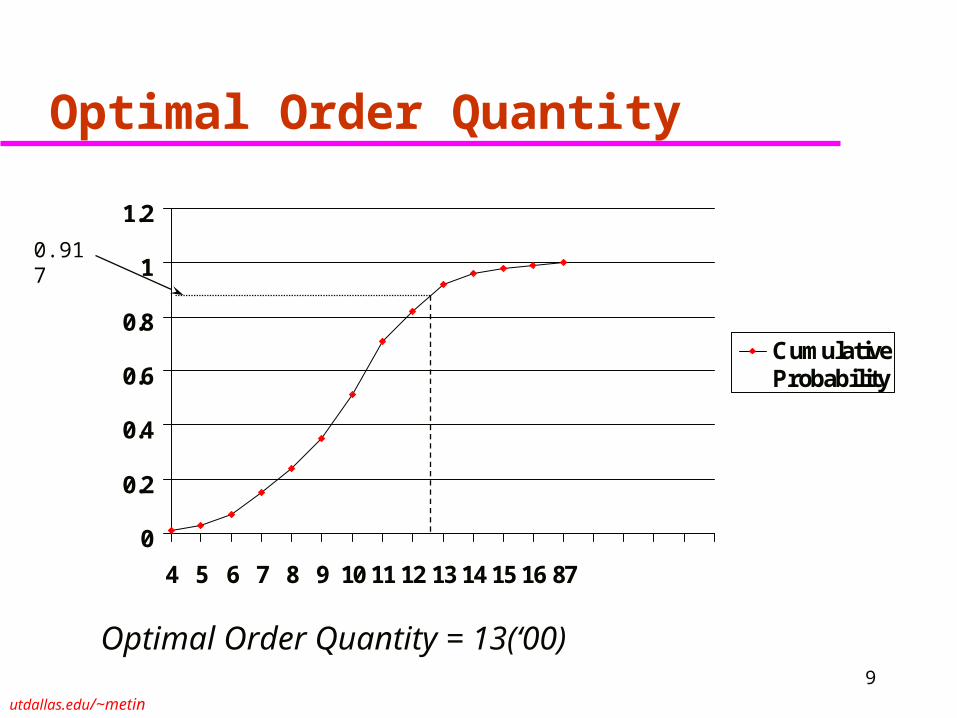
9
Optimal Order Quantity
0
0.2
0.4
0.6
0.8
1
1.2
4 5 6 7 8 9 10 11 12 13 14 15 16 87
CumulativeProbability
Optimal Order Quantity = 13(‘00)
0.917

utdallas.edu/~metin
10
Parkas at L.L. Bean
Expected demand = 10 (‘00) parkas Expected profit from ordering 10 (‘00) parkas = $499
Approximate Expected profit from ordering 1(‘00) extra parkas if 10(’00) are already ordered
= 100.55.P(D>=1100) - 100.5.P(D<1100)

utdallas.edu/~metin
11
Parkas at L.L. Bean
Additional100s
ExpectedMarginal Benefit
ExpectedMarginal Cost
Expected MarginalContribution
11th 5500.49 = 2695 500.51 = 255 2695-255 = 2440
12th 5500.29 = 1595 500.71 = 355 1595-355 = 1240
13th 5500.18 = 990 500.82 = 410 990-410 = 580
14th 5500.08 = 440 500.92 = 460 440-460 = -20
15th 5500.04 = 220 500.96 = 480 220-480 = -260
16th 5500.02 = 110 500.98 = 490 110-490 = -380
17th 5500.01 = 55 500.99 = 495 55-495 = -440

utdallas.edu/~metin
12
Revisit L.L. Bean as a Newsvendor Problem Total cost by ordering Q units:
– C(Q) = overstocking cost + understocking cost
Qu
Q
o dxxfQxCdxxfxQCQC )()()()()(0
0))(())(1()()(
uuouo CCCQFQFCQFCdQ
QdC
Marginal cost of raising Q* - Marginal cost of decreasing Q* = 0
uo
u
CC
CQDPQF
)()( **
Show Excel to compute expected single-period cost curve.
utdallas.edu/~metin
13
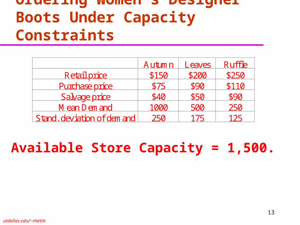
Ordering Women’s Designer Boots Under Capacity Constraints
Autumn Leaves Ruffle Retail price $150 $200 $250
Purchase price $75 $90 $110 Salvage price $40 $50 $90 Mean Demand 1000 500 250
Stand. deviation of demand 250 175 125
Available Store Capacity = 1,500.
utdallas.edu/~metin
14
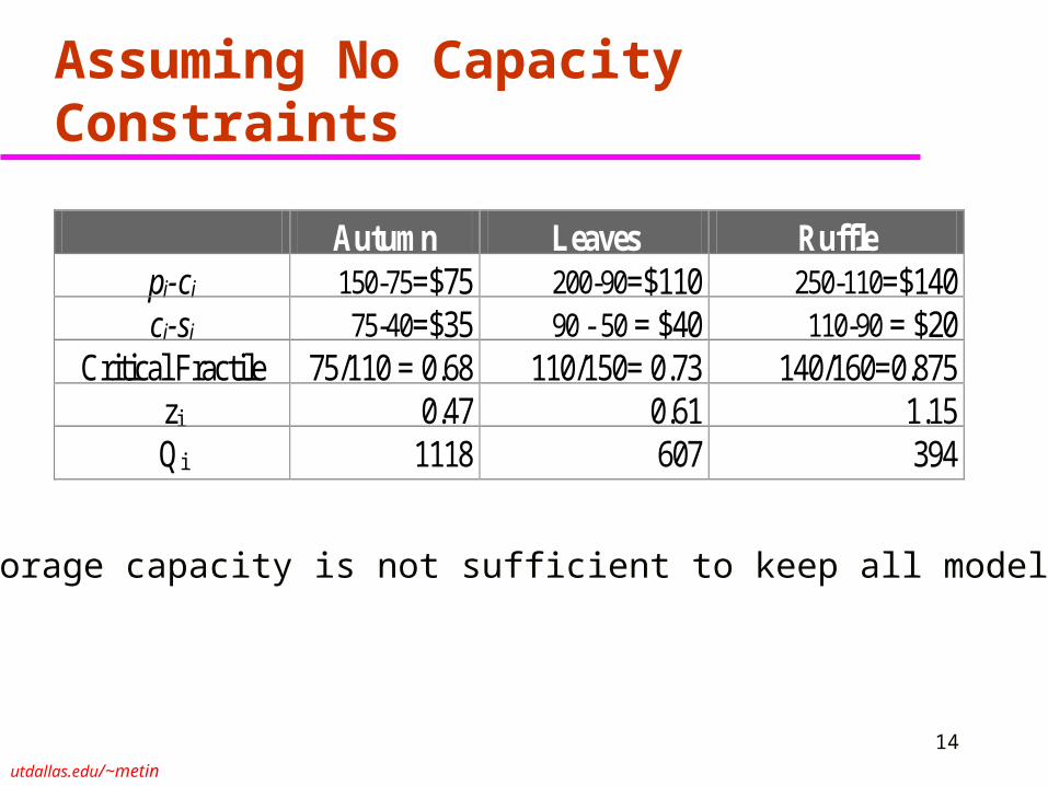
Assuming No Capacity Constraints
Autumn Leaves Ruffle pi-ci 150-75=$75 200-90=$110 250-110=$140 ci-si 75-40=$35 90 - 50 = $40 110-90 = $20
Critical Fractile 75/110 = 0.68 110/150= 0.73 140/160=0.875 zi 0.47 0.61 1.15 Qi 1118 607 394
Storage capacity is not sufficient to keep all models!

utdallas.edu/~metin
15
Algorithm for Ordering Under Capacity Constraints
{Initialization}
ForAll products, Qi := 0. Remaining_capacity:=Total_capacity.
{Iterative step}While Remaining_capacity > 0 do
ForAll products,
Compute the marginal contribution of increasing Qi by 1If all marginal contributions <=0, STOP{Order sizes are already sufficiently large for all products}else Find the product with the largest marginal contribution, call it j
{Priority given to the most profitable product}
Qj := Qj+1 and Remaining_capacity=Remaining_capacity-1
{Order more of the most profitable product}

utdallas.edu/~metin
16
Marginal Contribution=(p-c)P(D>Q)-(c-s)P(D<Q) Order Quantity Marginal Contribution
Remaining_Capacity Autumn Leaves Ruffle Autumn Leaves Ruffle 1500 0 0 0 74.997 109.679 136.360 1490 0 0 10 74.997 109.679 135.611
1360 0 0 140 74.997 109.679 109.691 1350 0 0 150 74.997 109.679 106.103 1340 0 10 150 74.997 109.617 106.103 1330 0 20 150 74.997 109.543 106.103 1320 0 30 150 74.997 109.457 106.103 1310 0 40 150 74.997 109.357 106.103
890 0 380 230 74.997 73.033 70.170 880 10 380 230 74.996 73.033 70.170 870 20 380 230 74.995 73.033 70.170
290 580 400 230 69.887 67.422 70.170 280 580 400 240 69.887 67.422 65.101
1 788 446 265 53.196 53.176 52.359 0 789 446 265 53.073 53.176 52.359

utdallas.edu/~metin
17
Optimal Safety Inventory and Order Levels:(ROP,Q) ordering model
Lead Times
time
inventory
Shortage
An inventory cycle
ROP
Q

utdallas.edu/~metin
18
A Cost minimization approach as opposed to the last chapter’s service based approach
Fixed ordering cost = S R / Q Holding cost = h C (Q/2+ss) where ss = ROP – L R Backordering cost (based on per unit backordered),
with f(.), the distribution of the demand during the lead time,
Total cost per time
ROP
dxxfROPxbQ
R)()(
per time
CostBackorder
ROP
per timeCostHolding
timeperCostOrdering
dxxfROPxQ
RbLRROP
QhC
Q
RS
)()(}2
{

utdallas.edu/~metin
19
Optimal Q (for high service level) and ROP
Q*=Optimal lot size ROP*=Optimal reorder point
A cost / benefit analysis to obtain CSL:– (1-CSL)bR/Q= per time benefit of increasing ROP by 1
» (1-CSL)b= per cycle benefit of increasing ROP by 1
– hC= per time cost of increasing ROP by 1– (1-CSL)bR/Q=hC gives the optimality equation for ROP
hC
SRQ
2* Rb
hCQROPFCSL 1)( **

utdallas.edu/~metin
20
Imputed Cost of Backordering
R = 100 gallons/week; R= 20; H=hC= $0.6/gal./year
L = 2 weeks; Q = 400; ROP = 300.
What is the “imputed cost” of backordering?
Let us use a week as time unit. H=0.6/52 per gal per week. Recall the formula
CSL = 1-HQ*/bR
per weekgallon per 8.230$100*0002.0
400*)52/6.0(
)1(
9998.0)1,2.28,200,300( ),,(
RCSL
HQb
normdistLRLROPFCSL R

utdallas.edu/~metin
21
Levers for Increasing Supply Chain Profitability Increase salvage value
» Obermeyer sells winter clothing in south America during the summer.» Sell the Xmas trees to Orthodox Christians after Xmas.» Buyback contracts, to be discussed.
Decrease the margin lost from a stock out– Pooling:
» Between the retailers of the same company. Ex. Volvo trucks.
» Between franchises/competitors. Franchises: Car part suppliers, McMaster-Carr and Grainger, are competitors but they buy from
each other to satisfy the customer demand during a stock out. Competitors: BMW dealers in the metroplex: Richardson, Dallas, Arlington, Forth Worth
– Dallas competes with Richardson so no pooling between them– Dallas pools inventory with the rest– Transportation cost of pooling a car from another dealer $1,500– Rebalancing: No transportation cost if cars are switched in the ship in the Atlantic
Improve forecasting to lower uncertainty Quick response by decreasing replenishment lead time which leads to a larger number of orders per
season Postponement of product differentiation Tailored (dual) sourcing

utdallas.edu/~metin
22
Impact of Improving ForecastsEX: Demand is Normally distributed with a mean of R = 350 and standard
deviation of R = 150Purchase price = $100 , Retail price = $250Disposal value = $85 , Holding cost for season = $5
How many units should be ordered as R changes?
Price=p=250; Salvage value=s=85-5=80; Cost=c=100
Understocking cost=p-c=250-100=$150, Overstocking cost=c-s=100-80=$20Critical ratio=150/(150+20)=0.88Optimal order quantity=Norminv(0.88,350,150)=526 units
Expected profit? Expected profit differs from the expected cost by a constant.

utdallas.edu/~metin
23
Computing the Expected Profit with Normal Demands
σ,1))μ,,normdist(Q(1 Q c)(p
σ,1)μ,,normdist(Q Q s)-(c -
)μ)/σ,0,1,0-Qnormdist(( σ s)-(p -
)μ)/σ,0,1,1-Qnormdist((μ s)-(p Profit Expected
σdeviation standard andμ mean with Normal is demand that theSuppose
dx f(x) Q)Profit(x,Profit Expected
Q xif c)Q-(p
Q xif x)-s)(Q-(c-c)x-(pQ)Profit(x,
quantity.order :Q f(x); pdf with demand :x
unit.per cost):c value;salvage :s price;:(p

utdallas.edu/~metin
24
Impact of Improving Forecasts
R Q* Expected
Overstock Expected
Understock Expected
Profit 150 526 186.7 8.6 $47,469
120 491 149.3 6.9 $48,476
90 456 112.0 5.2 $49,482
60 420 74.7 3.5 $50,488
30 385 37.3 1.7 $51,494
0 350 0 0 $52,500
Where is the trade off? Expected overstock vs. Expected understock. Expected profit vs. ?????

utdallas.edu/~metin
25
Cost or Profit; Does it matter?
optimal. same theyield they ;equivalent are Q)]E[Cost(x,Min and Q)],E[Profit(xMax
Qin Constant )c)E(Demand-(pQ)]E[Cost(x,Q)],E[Profit(x
c)x(pQ xifc)x -(p
Q xifc)x -(pQ)Cost(x,Q)Profit(x,
Q xif Q)-c)(x-(p
Q xif x)-s)(Q-(cQ)Cost(x,
Q xif c)Q-(p
Q xif x)-s)(Q-(c-c)x-(pQ)Profit(x,
quantity.order :Q f(x); pdf with demand :x
unit.per cost):c value;salvage :s price;:(p

utdallas.edu/~metin
26
Quick Response: Multiple Orders per Season
Ordering shawls at a department store– Selling season = 14 weeks (from 1 Oct to 1 Jan)– Cost per shawl = $40– Sale price = $150– Disposal price = $30– Holding cost = $2 per week
Expected weekly demand = 20 StDev of weekly demand = 15
Understocking cost=150-40=$110 per shawl Overstocking cost=40-30+(14)2=$38 per shawl Critical ratio=110/(110+38)=0.743=CSL

utdallas.edu/~metin
27
Ordering Twice as Opposed to Once
The second order can be used to correct the demand supply mismatch in the first order– At the time of placing the second order, take out the on-
hand inventory from the demand the second order is supposed to satisfy. This is a simple inventory correction idea.
Between the times the first and the second orders are placed, more information becomes available to demand forecasters. The second order is typically made against less uncertainty than the first order is.

utdallas.edu/~metin
28
Impact of Quick ResponseCorrecting the mismatch with the second order
Single Order Two Orders in a Season Service Level CSL
Order Size
Ending Invent.
Expect. Profit
Initial Order
OUL for 2nd Order
Ending Invent.
Average Total Order
Expect. Profit
0.96 378 97 $23,624 209 209 69 349 $26,590
0.94 367 86 $24,034 201 201 60 342 $27,085
0.91 355 73 $24,617 193 193 52 332 $27,154
0.87 343 66 $24,386 184 184 43 319 $26,944
0.81 329 55 $24,609 174 174 36 313 $27,413
0.75 317 41 $25,205 166 166 32 302 $26,916
OUL: Ideal Order Up to Level of inventory at the beginning of a cycle
Average total order approximately = OUL1+OUL2-Ending Inventory
As we decrease CSL, profit first increases, then decreases and finally increases again. The profits are computed via simulation.

utdallas.edu/~metin
29
Forecasts Improve for the Second Order Uncertainty reduction from SD=15 to 3
Single Order Two Orders in a Season Service Level
Order Size
Ending Invent.
Expect. Profit
Initial Order
OUL for 2nd Order
Average Total Order
Ending Invent.
Expect. Profit
0.96 378 96 $23,707 209 153 292 19 $27,007
0.94 367 84 $24,303 201 152 293 18 $27,371
0.91 355 76 $24,154 193 150 288 17 $26,946
0.87 343 63 $24,807 184 148 288 14 $27,583
0.81 329 52 $24,998 174 146 283 14 $27,162
0.75 317 44 $24,887 166 145 282 14 $27,268
With two orders retailer buys less, supplier sells less.
Why should the supplier reduce its replenishment lead time?

utdallas.edu/~metin
30
Postponement is a cheaper way of providing product variety
Dell delivers customized PC in a few days Electronic products are customized according to their distribution channels Toyota is promising to build cars to customer specifications and deliver
them in a few days Increased product variety makes forecasts for individual products inaccurate
– Lee and Billington (1994) reports 400% forecast errors for high technology products
– Demand supply mismatch is a problem» Huge end-of-the season inventory write-offs. Johnson and Anderson (2000) estimates
the cost of inventory holding in PC business 50% per year. Not providing product flexibility leads to market loss.
– An American tool manufacturer failed to provide product variety and lost market share to a Japanese competitor. Details in McCutcheon et. al. (1994).
Postponement: Delaying the commitment of the work-in-process inventory to a particular product, a.k.a. end of line configuration, late point differentiation, delayed product differentiation.

utdallas.edu/~metin
31
Postponement
Postponement is delaying customization step as much as possible
Need:– Indistinguishable products before customization
– Customization step is high value added
– Unpredictable demand
– Negatively correlated product demands
– Flexible SC to allow for any choice of customization step

utdallas.edu/~metin
32
Forms of Postponement by Zinn and Bowersox (1988)
Labeling postponement: Standard product is labeled differently based on the realized demand.– HP printer division places labels in appropriate language on to printers after the
demand is observed.
Packaging postponement: Packaging performed at the distribution center. – In electronics manufacturing, semi-finished goods are transported from SE Asia to
North America and Europe where they are localized according to local language and
power supply
Assembly and manufacturing postponement: Assembly or manufacturing is done after observing the demand.– McDonalds assembles meal menus after customer order.

utdallas.edu/~metin
33
Examples of Postponement HP DeskJet Printers
– Printers localized with power supply module, power cord terminators, manuals Assembly of IBM RS/6000 Server
– 50-75 end products differentiated by 10 features or components. Assembly used to start from scratch after customer order. Takes too long.
– Instead IBM stocks semi finished RS/6000 called vanilla boxes. Vanilla boxes are customized according to customer specification.
Xilinx Integrated Circuits– Semi-finished products, called dies, are held in the inventory. For easily/fast customizable
products, customization starts from dies and no finished goods inventory is held. For more complicated products finished goods inventory is held and is supplied from the dies inventory.
– New programmable logic devices which can be customized by the customer using a specific software.
Motorola cell phones– Distribution centers have the cell phones, phone service provider logos and service provider
literature. The product is customized for different service providers after demand is materialized.

utdallas.edu/~metin
34
Postponement Saves Inventory holding cost by reducing safety stock
– Inventory pooling
– Resolution of uncertainty
Saves Obsolescence cost Increases Sales Stretches the Supply Chain
– Suppliers
– Production facilities, redesigns for component commonality
– Warehouses

utdallas.edu/~metin
35
Value of Postponement: Benetton case
For each color, 20 weeks in advance forecasts– Mean demand= 1,000; Standard Deviation= 500
For each garment– Sale price = $50– Salvage value = $10– Production cost using option 1 (long lead time) = $20
» Dye the thread and then knit the garment
– Production cost using option 2 (short lead time) = $22» Knit the garment and then dye the garment
What is the value of postponement?– p=50; s=10; c=20 or c=22

utdallas.edu/~metin
36
Value of Postponement: Benetton case
CSL=(p-c)/(p-c+c-s)=30/40=0.75 Q=norminv(0.75,1000,500)=1,337
00,1))337,1000,5normdist(1(1 1337 20)(50
00,1)337,1000,5normdist(1 1337 10)-(20 -
0,1,0)1000)/500,-1337normdist(( 500 10)-(50 -
0,1,1)1000)/500,-1337normdist(( 1000 10)-(50 Profit Expected
Expected profit by using option 1 for all products4 x 23,644=$94,576

utdallas.edu/~metin
37
Apply option 2 to all products: Benetton case
CSL=(p-c)/(p-c+c-s)=28/40=0.70 Demand is normal with mean 4 x 1000 and st.dev sqrt(4) x 500 Q=norminv(0.75,4000,1000)=4524
000,1))524,4000,1normdist(4(1 4524 22)(50
000,1)524,4000,1normdist(4 4524 10)-(22 -
,0,1,0)4000)/1000-4524normdist(( 1000 10)-(50 -
,0,1,1)4000)/1000-4524normdist(( 4000 10)-(50 Profit Expected
Expected profit by using option 2 for all products=$98,902
utdallas.edu/~metin
38
Postponement Downside
By postponing all three garment types, production cost of each product goes up
When this increase is substantial or a single product’s demand dominates all other’s (causing limited uncertainty reduction via aggregation), a partial postponement scheme is preferable to full postponement.

utdallas.edu/~metin
39
Partial Postponement: Dominating Demand Color with dominant demand: Mean = 3,100, SD = 800 Other three colors: Mean = 300, SD = 200
Expected profit without postponement = $102,205 Expected profit with postponement = $99,872
Are these cases comparable?
– Total expected demand is the same=4000
– Total variance originally = 4*250,000=1,000,000
– Total variance now=800*800+3(200*200)=640,000+120,00=760,000
Dominating demand yields less profit even with less total variance. Postponement can not be any better with more variance.

utdallas.edu/~metin
40
Partial Postponement: Benetton case
For each product a part of the demand is aggregated, the rest is not Produce Q1 units for each color using Option 1 and QA units
(aggregate) using Option 2, results from simulation:
Q1 for each QA Profit
1337 0 $94,576
0 4524 $98,092
1100 550 $99,180
1000 850 $100,312
800 1550 $104,603

utdallas.edu/~metin
41
Tailored (Dual) Sourcing
Tailored sourcing does not mean buying from two arbitrary sources. These two sources must be complementary: – Primary source: Low cost, long lead time supplier
» Cost = $245, Lead time = 9 weeks
– Complementary source: High cost, short lead time supplier» Cost = $250, Lead time = 1 week
An example CWP (Crafted With Pride) of apparel industry bringing out competitive advantages of buying from domestic suppliers vs international suppliers.
Another example is Benetton’s practice of using international suppliers as primary and domestic (Italian) suppliers as complementary sources.
utdallas.edu/~metin
42
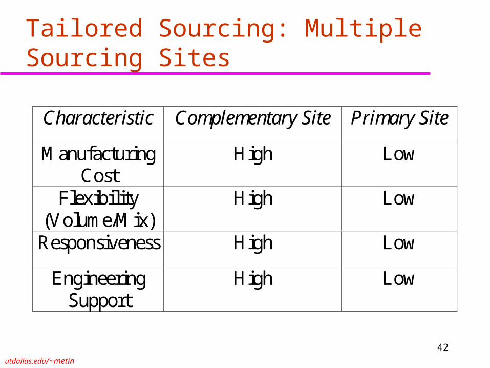
Tailored Sourcing: Multiple Sourcing Sites
Characteristic Complementary Site Primary Site
Manufacturing Cost
High Low
Flexibility (Volume/Mix)
High Low
Responsiveness High Low
Engineering Support
High Low

utdallas.edu/~metin
43
Dual Sourcing Strategies from the Semiconductor Industry
Strategy Complementary Site Primary Site
Volume based dual sourcing
Fluctuation Stable demand
Product based dual sourcing
Unpredictable products, Small
batch
Predictable, large batch products
Model based dual sourcing
Newer products Older stable products

utdallas.edu/~metin
44
Learning Objectives Optimal order quantities are obtained by
trading off cost of lost sales and cost of excess stock
Levers for improving profitability– Increase salvage value and decrease cost of stockout
– Improved forecasting
– Quick response with multiple orders
– Postponement
– Tailored sourcing


