UvA-DARE is a service provided by the library of the University of Amsterdam (http://dare.uva.nl)

UvA-DARE (Digital Academic Repository)

Nonparametric Prediction: Some Selected Topics

Zerom Godefay, D.

Link to publication

Citation for published version (APA):Zerom Godefay, D. (2002). Nonparametric Prediction: Some Selected Topics

General rightsIt is not permitted to download or to forward/distribute the text or part of it without the consent of the author(s) and/or copyright holder(s),other than for strictly personal, individual use, unless the work is under an open content license (like Creative Commons).

Disclaimer/Complaints regulationsIf you believe that digital publication of certain material infringes any of your rights or (privacy) interests, please let the Library know, statingyour reasons. In case of a legitimate complaint, the Library will make the material inaccessible and/or remove it from the website. Please Askthe Library: http://uba.uva.nl/en/contact, or a letter to: Library of the University of Amsterdam, Secretariat, Singel 425, 1012 WP Amsterdam,The Netherlands. You will be contacted as soon as possible.

Download date: 11 Jun 2018

Chapterr 5

Multi-stagee Conditional Quantile

Prediction n

5.11 Introduction

Lett {Wt;t ^ 1} be a real-valued strictly stationary time series. Of particular interest

iss to predict future values W^+H for H = 1,2,... from observed values WN, Wjv-i ,

Inn fact, this was the goal of Chapter 2. With the same objective in mind, the present

chapterr is aimed at improving the multi-step ahead prediction accuracy of the kernel-

basedd prediction methods. One unattractive feature of most nonparametric prediction

methodss (including the ones discussed in Chapter 2) is that, when making more than

one-stepp ahead (H ^ 2) predictions, not all the information contained in the past is

efficientlyy used. Thus a substantial loss in prediction accuracy is likely to occur.

Inn this chapter, we address this shortcoming when a time series is Markovian and

considerr the case of quantile prediction. Our proposed solution involves a careful but

directt use of the Markovian property of the time series.1 By so doing, it turns out that

onee or more of the unused data can be easily incorporated in a recursive manner while

improvingg prediction efficiency in the sense of improved variance. Motivated by this

recursionn idea, we propose a multi-stage kernel smoother for conditional quantiles. We

alsoo show theoretically that the asymptotic performance of the new predictor is superior

too the corresponding single-stage conditional quantile estimator in terms of mean squared

errorr (MSE). We like to note that, in principle, the ideas discussed in this chapter can also

bee directly adapted to predictors like the conditional mean and the conditional mode.

'Notee here the analogy with the approach in Chapter 4 where the conditional quantile, 0a(x) assumes

ann additive structure and we exploited that structure to achieve: (a) a better convergence rate, and (b)

ann interpretation feature of the linear model.

71 1

72 2 ChapterChapter 5: Multi-stage Conditional Quantile Prediction

Thee remainder of the chapter is structured as follows. In Section 5.2 we clarify the

differencee in information content used by the estimators of the single-stage and the multi-

stagee conditional quantiles. Section 5.3 contains the main result stating that the estimator

off the two-stage conditional quantile has a smaller asymptotic MSE than the estimator

off the single-stage conditional quantile. Empirical comparison of the single-stage and

multi-stagee predictors of the conditional quantile via a simulation study is carried out in

Sectionn 5.4. In Section 5.5 we evaluate the two prediction approaches in an application to

thee changes in the U.S. monthly interest rate series. Conditions and proofs are collected

inn Section 5.6. Section 5.7 closes the chapter with some concluding remarks.

5.22 Single-stage versus multi-stage prediction

Lett {Wt; t ^ 1} be a Markovian process of order m, i.e. C{Wt\Wt_u ..., W{)= £,{Wt\Wt-i,

, Wt-m) where C denotes the law. From the set of observations Wx,..., WN, we are

interestedd in making predictions of W^+H where H (1 ^ H ^ N - m) denotes the

predictionn horizon. For that purpose, we construct the associated process (Xt, Zt) defined

by y

XXtt = (Wt, Wt+U ..., W W i ) , Zt = H W h m - i, (* = 1, , n) (5-1)

wheree n = N -H -m+1. Let {(X, , Z(; £ ^ 1)} be a sequence of Rm x E valued strictly

stationaryy random variables with common probability density function with respect to

thee Lebesgue measure Am+1 on Rm+1.

Now,, given observations (Xu Zi),..., (X„ , Z„) , where n = N-H-m+l, an estimator

66ayayn{x)n{x) of the true quantile Ba(x) can be defined as the root of the equation Fn(z\x) = a

wheree F„(-\x) is an estimator of F(-\x). Thus a predictor of a th conditional quantile

off WN+H is given by 9a^n(XN-m+i)- In this Chapter, for the estimation of F{-\x), we

shalll use the well-known Nadaraya-Watson smoother (see also Chapters 2 and 4) which

iss re-introduced here for clarity of presentation:

FF^^x)x) = TL^Hx-x.yh.y (5'2)

wheree 1^ denotes the indicator function for set A, K(-) is a nonnegative density function

(kernel),, and hn is the bandwidth. The result of the current chapter continues to hold if we

aree to consider other kernel smoothers of F(*|a;) such as the re-weighted Nadaraya-Watson

method;; see Chapter 4.

Multi-stageMulti-stage Conditional Quantile Prediction 73 3

Wee shall refer to the solution of the equation

F(z\x)F(z\x) = Q (5.3)

ass the single-stage conditional quantile predictor and denote this by 8Q(x). Note that

thee conditional quantile predictor in (5.3) uses only the information in the pairs (Xt, Zt)

(t(t = 1 , . . ., n) and ignores the information contained in

YlYll)l) = Xt+u Yf)^Xw,...^i-x)=Xt+{H )̂. (5.4)

Beloww we illustrate the impact of the data contained in (5.4) on multi-step prediction

accuracy.. Let Qi(y) = E(l{Zt̂ z}\Y[H~ — y). For j = 2, ...,H~ 1, also define

Qj{y)Qj{y) = E(Qj_i(Yt ~ )\Y't J — y). It is well-known that for a pair of random

variabless (B ,C), Var(C) = E[Var{C\B)] + Var[E{C\B)]. Hence, VarlQ^Y^'^)} =

Var [£7(öi (K i " - i ) ) | l r i f f - i - 1 )) ]+£; [Var(öJ- ( l r i / ' " J' ) ) | r iH - - j - 1 )) ] .. But, for j = 1,.. .,H-2,

wee have G^Y?-^) = E ^ Y ^ ) ^ " - ^ ). Thus

Var[gVar[gj+1j+1 (Y[(Y[HH--jj--l)l))])] ̂VarfaiY?-»)]. (5.5)

Similarly,, it is also easy to see that

Var\gVar\gll{Y\{Y\HH--l)l))\X)\Xtt = x] ̂Var[l {ZKz}\Xt = a;]. (5.6)

Now,, directly exploiting the Markovian property of Wt, we can rewrite E(l{Zt̂ z}\Xt = x)

inn such a way that the information in (5.4) is incorporated, i.e.

E(lE(l{Zt{Zt** s}s}\X\Xtt = x) = E{gl(Y\H-1))\Xt = x),

== E(G2{Y^-2))\Xt = xl I 5-7) )

== E{GH-i{Y(p)\Xt = x).

Observee that as we go down each line in (5.7) more and more information is utilized. Re-

callingg the two previous inequalities, (5.5) and (5.6), we can see that as more information

iss used, the prediction variance gets smaller and hence prediction accuracy, in terms of

MSEE improves. Thus, at least in theory, it pays off to use all the ignored information.

Basedd on the above recursive set-up, we now introduce a kernel-based estimator of

F(z\x).F(z\x). First the estimators of Q\{y) and Gj(y), {j = 1,... ,H — 2) are defined, respec-

744 Chapter 5: Multi-stage Conditional Quantile Prediction

tively,, as follows

t = i i Stagee 1: Qx{y) =

E^{(2/-nH- j ) )/^>tó-i(^-0-1,); ; Stagee j : ^(3/) =

Then,, using Gn-i(y), we compute F(z\x) by

n n

Staged:: F{z\x) = ̂ s . (5.8)

^ X { ( x - X f c ) / W W

Wee shall refer to the root of the equation F(z\x) — a as the multi-stage a-conditional

quantilee predictor #n(x).

5.33 Asymptot ic MSEs

Beforee comparing the asymptotic MSE of the multi-stage conditional quantile smoother

withh the asymptotic MSE of the single-stage conditional quantile smoother, we first

presentt some results on the asymptotic properties of conditional quantiles. To this end,

wee assume for simplicity of notation that H — 2, and m = 1. Prom the process (Wi), let

uss construct the associated process £/, — (Xi,Yi,Zi) defined by

XiXi = Wh Yi = Y ̂ = Wi+U Z{ = Wi+2.

Wee suppose that the random variables (X, Y) (respectively (Y, Z)) has a joint density

PX,Y(',PX,Y(', ) (respectively PY,Z(-, Let g(x), g(y) and g(z) be the marginal densities of X,

Y,Y, and Z, and f{-\x) = Px,z{x, ')/g(x) be the conditional density function. Furthermore,

wee define

Multi-stageMulti-stage Conditional Quantile Prediction 75 5

Givenn the above set-up, and using the conditions given in Section 5.6, the following

Lemmass and Theorems can be stated.

Lemmaa 1: (Collomb, 1984; Hall, Wolff and Yao, 1999): Let (X,Z) be R2-valued

randomrandom variables. For z E R, define a2(z,x) — Var(l{z^z}\X = x). Assume that

ConditionsConditions A.l-A.3 given in Section 5.6 are satisfied. If'nhn — oo, then

MSE{F(z\x)}MSE{F(z\x)} = ~D2(zyx)+KDf'x) + o(h* + - U nnnnnn 4 \ nnnJ

Dl („ )) = ^{F^(, W + ̂ » l } 2 , (5.9)

11 „ , , , KD^x)

where where

DA?DA? T\ = k2\ F^UrM +

kk22aa22(z,x) (z,x) DD22{z,x){z,x) = T-—,

andand where ki and k2 are constants defined respectively as k\ — J u2K{u)du and k2 =

fKfK22(u)du. (u)du.

Theoremm 1: Assume that Conditions A.l-A.6 given in Section 5.6 are satisfied. If

nhnhnn —> oo as n —> oo, then for all I É R , the asymptotic pointwise MSE of 0a(x) is given

by by

MSMS** èè-™-™ a 7^^(^;W-^J^( W , . ) ). (5.io)

Furthermore,Furthermore, under the same conditions mentioned above and if Di(8a(x),x) ̂ 0, the

asymptoticallyasymptotically optimal value h*n, say ofhn, minimizing (5.10) is given by

, .. _ (D2(0«(x)tx)y/z _1/5

andand the corresponding best possible MSE of 9n{x) is given by

c n - 4 /5 5 MSET{0MSET{0aa(x)}(x)} ~ 4f2{e(i{x)lx)

D2\U^)^)Dl/5(ea(x),x).

Remarkk 1: Using Lemma 1 above and Theorem 4 in Cai (2000), Theorem 1 follows.

Similarr results can be found in Berlinet et al. (2001) and Jones and Hall (1990).

Lemmaa 2: Under Conditions A.I A.5, for any cn —> 0,

F(zF(z + cn\x) - F(z\x) = f{z\x)c» + op(cn) + op((nh2tn)~1/2). (5.11)

76 6 ChapterChapter 5: Multi-stage Conditional Quantile Prediction

T h e o r e mm 2: Assume that Conditions A.l-A.6 are satisfied, and that nh\ n̂ —> oo as

nn —Y ooo and in = o(/i2,n)- For 2 É 1 , /e£ Ui(z,x) = Ka r f ^ i f y ) ^ ) (Q\{Y) is as defined

inin Section 5.2). Then for all x E IR, we have

(i) (i)

hhAA 1 A/St f l fYdx) }} ~ -^-DAz,x) + ——D-Az^x)

44 nh'2,,,

where where

D,(z,x)D,(z,x) = k 2V ^ - . (5.12)

(it)(it) The two-stage estimator is point-wise consistent, i.e.

00aa(x)=9(x)=9aa{x)+o{x)+opp{l). {l).

(in)(in) The best possible asymptotic MSE of 9a{x) is given by

MSE*{êMSE*{êaa{x)}{x)} ~ E ) ^ ) ^ i 1 / 5 ( ^ ( - r ) ^ ) ) -

Corollary:: Let v-2(z,x) — is jVarf l^^i lF)! :* ; ] . Then, under the conditions of Theorems

11 and 2, the ratio of the asymptotic best possible MSEs (or MSE*s) of the single-stage

estimatorestimator 6n(x) and the two-stage estimator 9a(x) is given by

» 2 ( » „ ( I ) , J : ) I < / 5 5

ii vi(ea(x),x))

Remarkk 2: Note that the asymptotic results are insensitive to the choice of the band-

widthh hi<n, provided nhii7l —> oo and hi,n = o(h-2,n)-

Remarkk 3: It can be noticed from the proof of the Corollary that the asymptotic MSE of

thee two-stage smoother is smaller because vi(q(x), x) ^ a2(q(x), x); see also the discussion

inn Section 5.2.

Remarkk 4: It can easily be verified that o-2(9a(x),x) = Q (1 — a). Further, note that

aa22(6(6nn(x),x)(x),x) = vi(6n(x),x)+V2{6a{x),x). Thus we express the asymptotic ratio r(9a(x),x)

ass a function of a: r — {a( l — a ) / ( a (l — a) — i^)} 4^5- Note that v2 ^ a(\ — a). Figure 5.1

Multi-stageMulti-stage Conditional Quantile Prediction 77 7

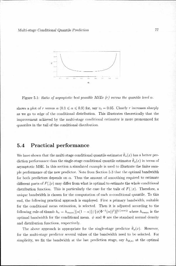
Figuree 5.1: Ratio of asymptotic best possible MSEs (r) versus the quantile level a.

showss a plot of r versus a (0.1 ^ a ^ 0.9) for, say v2 = 0.05. Clearly r increases sharply

ass we go to edge of the conditional distribution. This illustrates theoretically that the

improvementt achieved by the multi-stage conditional estimator is more pronounced for

quantiless in the tail of the conditional distribution.

5.44 Practical performance

Wee have shown that the multi-stage conditional quantile estimator 9a(x) has a better pre-

dictionn performance than the single-stage conditional quantile estimator 9a(x) in terms of

asymptoticc MSE. In this section a simulated example is used to illustrate the finite sam-

plee performance of the new predictor. Note from Section 5.3 that the optimal bandwidth

forr both predictors depends on a. Thus the amount of smoothing required to estimate

differentt parts of F(.|a:) may differ from what is optimal to estimate the whole conditional

distributionn function. This is particularly the case for the tails of F(.\x). Therefore, a

uniquee bandwidth is chosen for the computation of each «-conditional quantile. To this

end,, the following practical approach is employed. First a primary bandwidth, suitable

forr the conditional mean estimation, is selected. Then it is adjusted according to the

followingg rule-of-thumb hn - hmean[{a(l - a) } / {0($ _ 1(a) )2} ] 1 / ( m + 4) where hmean is the

optimall bandwidth for the conditional mean. <fi and <3> are the standard normal density

andd distribution functions, respectively.

Thee above approach is appropriate for the single-stage predictor 9a(x). However,

forr the multi-stage predictor several values of the bandwidth need to be selected. For

simplicity,, we fix the bandwidth at the last prediction stage, say hH,n, at the optimal

78 8 ChapterChapter 5: Multi-stage Conditional Quantile Prediction

valuee of the single-stage estimator hn. The bandwidths in the intermediate stages are

scaledd downward arbitrarily vis-a-vis hn,n- This is in accordance with the theory of

Sectionn 5.3. Different options such as hH,n, ^ff,n/5, hIIiTl /lO, and hHtn/20 were tried and

thee last three seem to give more or less similar results. Hence only results for /i//,„/ 5 are

reported.. The standard Gaussian kernel is used throughout all computations.

Considerr the simple, Markovian type, nonlinear autoregressive model of order 1

ZZ(( = 0 .232^(16 - Zt_x) + 0Aet (5.13)

wheree {et} is a sequence of i.i.d. random variables each with the standard normal dis-

tributionn truncated in the interval [-12,12]. The objective is to estimate 2- and 5-step

aheadd a-conditional quantiles using both O^x) and 9a(x) and compare their prediction

accuracy.. Predictions wil l be made at a — 0.25, a = 0.50, and a — 0.75. The condi-

tionall density of Zt+H given Zt — x wil l be examined at x — 6, x — 8, and x — 10,

Clearlyy a proper evaluation of the accuracy of 0a(x) and 9a(x) requires knowledge about

thee "true" conditional quantile 9a(x). This information is obtained by generating 10,000

independentt realizations of (Zt+H\Zt - x) (H=2, and 5) iterating the process (5.13) and

computingg the appropriate quantiles from the empirical conditional distribution function

off these generated observations.

Fromm (5.13), 150 samples of sample size n=150 were generated. Each replication had

aa unique seed. To compare the accuracy of the predictors 9a(x) and 9a(x) with 9a(x),

thee following error measures are computed for each replication j (j = 1 , . . ., 150):

dd ={K(x)-ea(x)¥ and e, _{êj(x)-9a(x)y

Thenn percentile values are computed from the empirical distributions of the 150 replication

samples,, i.e. from e{ , , and e{ , ,.

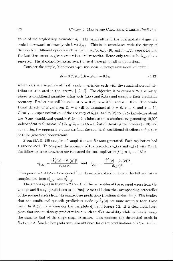
Thee graphs a)-c) in Figure 5.2 show that the percentiles of the squared errors from the

2-stagee and 5-stage predictions (solid line) lie overall below the corresponding percentiles

off the squared errors from the single-stage predictions (medium dashed line). This implies

thatt the conditional quantile predictions made by 9a(x) are more accurate than those

madee by 9a(x). Now consider the box plots d)-f) in Figure 5.2. It is clear from these

plotss that the multi-stage predictor has a much smaller variability while its bias is nearly

thee same as that of the single-stage estimator. This confirms the theoretical result in

Sectionn 5.3. Similar box plots were also obtained for other combinations of H, a, and x.

Multi-stageMulti-stage Conditional Quantile Prediction 79 9

)) H=2,a=0.75,x=6 d)H=2,a=0.75,x=6 6

99 "*''

^ y ' '

// . // / // / // /

I I 1/ 1/

1 1 1 1

/ / 1 1

Peicentte e

ta)H=5,a=0.75,x=10 ta)H=5,a=0.75,x=10

/ / / / // / // -̂-̂ / > ^ ^

/ / / / // /

/ / / / / / /-"" /

II H = 5,a=0.75,x=10

0 0 o o

o o

1 1

:

o o

T T

L ? ? HH = 5 ,a=025.x=6

Figuree 5.2: a)-c) Percentile plots of the empirical distribution of the squared errors

forfor model (5.13) for the single-stage predictor 6a(x) (medium dashed line) and the

multi(=two)-stagemulti(=two)-stage predictor 6a(x) (solid line); d)-f) Box plots corresponding to the per-

centilecentile plots a)-c), respectively; n — 150, 150 replications.

80 0 ChapterChapter 5: Multi-stage Conditional Quantile Prediction

5.55 Application

Heree we apply the multi-stage and single-stage conditional quantile predictors to obtain

6-stepp ahead out-of-sample prediction intervals for the monthly U.S. short-term interest

rate,, i.e. the yield on U.S. Treasury Bill s with three months to maturity. The time

seriess contains 348 monthly observations from January 1966 to December 1994. The first

differencee of the original series (after taking logarithms), denoted by Wt, wil l be used in

ourr analysis with a total of 347 observations. Using the notations of Section 5.2, Xt = Wt

andd Zt = Wt+g where t = 1 , . . ., N — 6, and N is the index of the prediction base. In

thiss example, a nominal coverage probability of 0.80 is considered, i.e. [0o.i{x),6o.g(x)]

wheree x = XN. Note that 60A(x) and #0.9(0:) are respectively the 6-step ahead 10th- and

90th-conditionall quantiles.

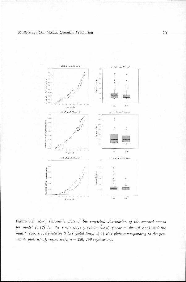
Ass in Section 5.4, we choose he,n such that /i6,„, = hn where hn is the optimal value of

thee single-stage estimator. In the intermediate stages, the theory requires the bandwidths

bee smaller than /i6jr,. In order to have some idea on how smaller they should be, we

computee in-sample 6-step ahead predictions at various levels of undersmoothing (i.e.,

he,,i/5,he,,i/5, h6tn/10, h6y„/15,... ,/iBlU /70). By in-sample, it is meant that x 6 Xt. Among

variouss bandwidths considered, the choice: hit„ = /i6,n/45 and /i2,n = h n̂ = hi<n = h n̂ =

/i 6j„/355 seems to yield multi-stage quantile estimates (see Figure 5.3) which are roughly

thee same as that of the single-stage while being less noisy.

Figuree 5.3: In-sample 10th- and 90th-conditional quantile estimates of the single-stage

(medium(medium dashed line) and the multi-stage (solid line) predictors.

Noww using the above set of bandwidths, we compute 6-step ahead out-of-sample pre-

dictionss standing on the last 42 observations, i.e. H^oo,- • •, WMI- For example, at W30o

Multi-stageMulti-stage Conditional Quantile Prediction 81 1

0:055 -

0.000 -

-0.00 5 -

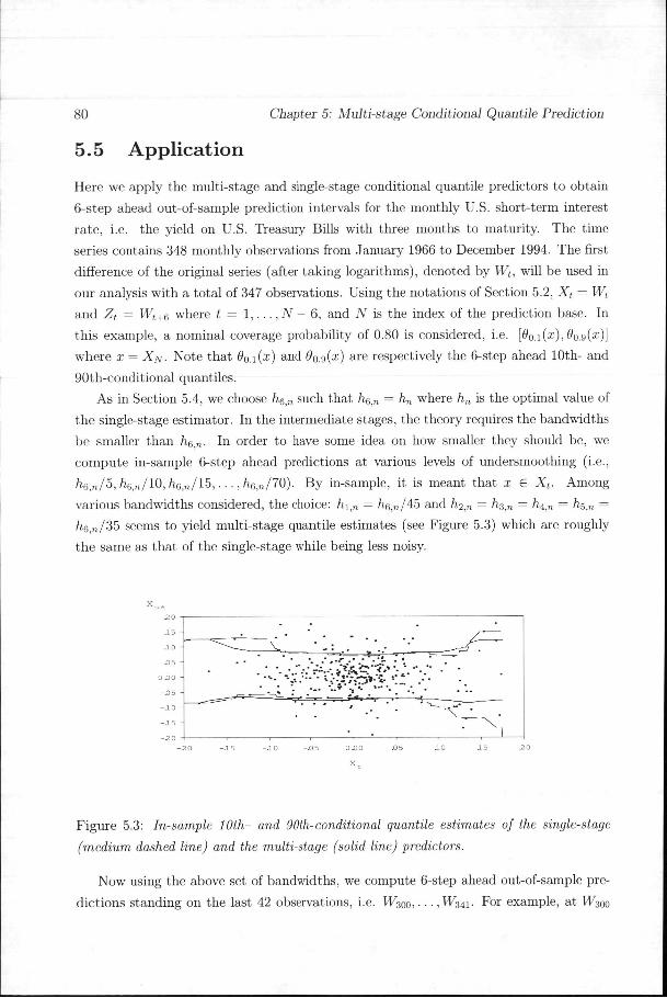
Figuree 5.4: Out-sample 10th- and 9Oth-conditional quantile estimates of the single-stage

(medium(medium dashed line) and the multi-stage (solid line) predictors.

wee predict the 10th or 90th quantile of W306 conditional on x = X300. The respective

averagee lengths of the intervals for the single-stage and multi-stage are 0.148 and 0.152

which,, respectively, are 24% and 25% of the range of the data. Thus both estimators

performm comparably well in the sense of having not too wide intervals. Only about 19%

off the actual observations lie outside the intervals. The average values of the upper and

lowerr predictive intervals for the single-stage and multi-stage are [-0.0719 (0.0125); 0.0759

(0.0175)]] and [-0.0755 (0.0038); 0.0765 (0.0095)], respectively, where the numbers in the

parenthesess are the standard deviations. This indicates that the single-stage based con­

fidencefidence intervals are more erratic than those of the multi-stage approach. We can also

observee this from Figure 5.4 which displays the 80% confidence intervals.

Inn the foregoing analysis we have used quantiles to construct the confidence intervals.

Butt in situations where the predictive densities are asymmetric or multi-modal, the quan­

tilee based intervals tend to give wider intervals. To deal with this problem, we introduced

inn Chapter 2 two efficient predictive intervals (SCMI and MCDR) which are based directly

onn the conditional distribution function (CDF). Fortunately, the multi-stage approach in­

troducedd in the current chapter is still useful. We just have to employ the multi-stage

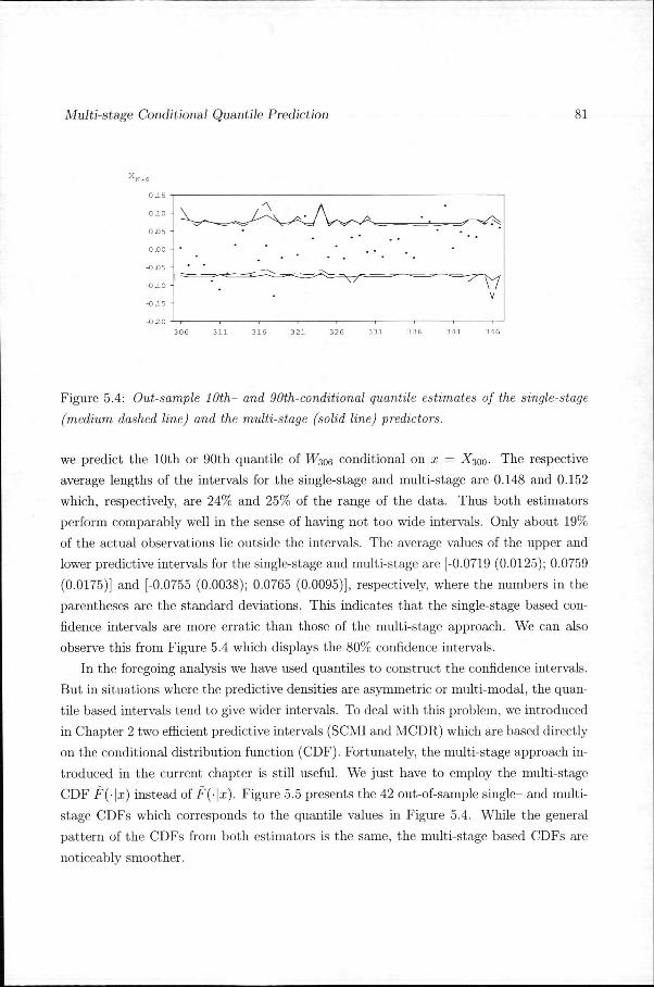
CDFF F(-\x) instead of F(-\x). Figure 5.5 presents the 42 out-of-sample single- and multi­

stagee CDFs which corresponds to the quantile values in Figure 5.4. While the general

patternn of the CDFs from both estimators is the same, the multi-stage based CDFs are

noticeablyy smoother.

82 2 ChapterChapter 5: Multi-stage Conditional Quantile Prediction

-OO £ -0 3 -O A - 0 3 -0 2 -O JL 0 .0 01 02 03 0-4

-OO .6 -O 3 -0-4 -O 3 - 0 .2 - 0 . 1 0:0 O J 0 2 0 3 0 A

Figuree 5.5: a) 42 out-of-sample single-stage CDFs; b) 4% out-of-sample multi-stage CDFs.

5.66 Conditions and proofs

Thee asymptotic results will be derived on a set of conditions gathered below for ease of

reference. .

A.ll The sequence {[/ , ; i ^ 1} is strongly mixing (a-mixing); see Section 3.3 for defini­

tion. .

A.22 The kernel K is compactly supported, symmetric density function.

A.33 For fixed z and x, g(x) > 0, 0 < F(z\x) < 1, g(-) is continuous at x, and F(z\x) has

continuouss second derivative with respect to x.

A.44 Assume that F(z\x) has a conditional density f(z\x) and f(z\x) is continuous at x.

A.55 f(ea(x)\x) > 0.

A.66 8a(x) exists and is unique.

Forr ease of notation we replace X = x by x in the following proofs.

Prooff of L e m m a 2. For clarity of presentations lets repeat the definition of F(z\x)

notingg that we are dealing with H = 1 case:

S = i ^ 2 > - * * ) ê i ( n ) ) F(z\x) F(z\x)

Y2=lY2=lKKh2.n(h2.n(XX--XXk k (5.14) )

Multi-stageMulti-stage Conditional Quantile Prediction 83 3

where e

l[y)l[y) YJUK^y-Yi) •

Noticee that G\(y) = F{z\y). Then from Lemma 1 we have

F(z\y)F(z\y) = F(z\y) + op(l)

ass nhi,n -> oo for n —»• oo. It can also be shown that g(x) = g(x) + op(l) . Thus, (5.14)

becomes s n n

F(z\x)F(z\x) = n-lg-l{x) £ i ^ 2 n(x - Xk)F{z\Yk){\ + op(l)}. fc=i fc=i

Usingg the above result, we have that

F(zF(z + cn\x) - F(z\x) = n~l ] T Kh,Jx - Xk) \F{Z + cn\Yk) - F{z\Yk)\g-\x){\ + o p ( l )} . fe=i fe=i

Noww Taylor expanding F(z + cn\Yk) about z, we obtain

F{zF{z + cn\x) - F(z\x) = Jg-\x){l + op(l)} (5.15)

wheree J = n~l Y^k=\ Kh2,,Ax ~ Xk)\f(z\Yk)cn + o(cn) . Prom routine calculations, we

havee that E (J) = f(z\x)g(x)cn + o(cn). Similarly, Var(J) = 0{cn{nh2,n)~1)- Therefore,

JJ = f(z\x)g(x)cn + op(cn) + op((nh2,n)~l/2)-

This,, together with (5.15), proves the Lemma.

Sketchh proof of Theorem 2.

i)) Combining results from Roussas (1991, Theorem 2.3) and Chen (1996, Theorem 1)

andd using Conditions A.l - A.5, and Davydov's inequality (see Section 3.4), one can

obtainn the asymptotic normality of Fn(z\x):

(nh(nh22̂ [F^[F MMx)x) - F(z\x) - % f c l { i ^ > ( * | z ) + 2 g { 1 ) ( y ( z | g ) } ]

-^- ̂ Af{0,D3{z,x)) (5.16)

wheree D3(z,x) is as defined in (5.12). From the above result, it follows directly that

thee asymptotic MSE of F(z\x) is given by

hhAA 1 MSE{F(z\x)}MSE{F(z\x)} ~ -JfiD^z.x) + ——Di{z,x)

44 nh2,n

wheree Di(z,x) is as defined in (5.9).

84 4 ChapterChapter 5: Multi-stage Conditional Quantile Prediction

ii)) By Condition A.6, F(-\x) has a unique quantile, 9Q(x), of order a. Thus, for any

f.f. > 0, there exists 77(e) > 0 defined by

rj(e)rj(e) = min ( F ( # Q (X ) + e\x) - F(6a{x)\x), F(0a(x)\x) - F{$n{x) - c|x))

suchh that

Ve>00 V Z G R \da{x)-z\^t^\F{0a{x)\x)-F{z\x)\^7]{e).

Now w

\F0\F0aa(x)\x)(x)\x) - F{0a{x)\x)\ ̂ \F(Ba{x)\x)-F(9a{x)\x)\ +

\F{8\F{8aa{x)\x){x)\x) - F(9a{x)\x)\

^ ̂ \F(9a(x)\x) - F(0a(x)\x)\

<< sup\F{z\x)-F(z\x)\. (5.17)

Wee know from Theorem 2(i) that F(z\x) = F(z\x) + op{\). Because F(z\x) is a

distributionn function, it also follows that

sup\F{z\x)-F(z\x)\sup\F{z\x)-F(z\x)\ ^ 0 (5.18) ces s

Combiningg (5.17), (5.18) and the following inequality:

P{\0P{\0aa(x)(x) - 9a(x)\ ^e} ̂ P fsup \F(z\x) - F(z\x)\ > V(e)),

wee can see that 9a(x) — 6a(x)+op(l). Thus the proof of Theorem 2(ii) is complete.

(iii)) Now we apply Lemma 2. Let z = 9a(x) and cn = 0n(x) - 9a(x). Notice that the

requirementt cn —> 0 is satisfied from Theorem 2(ii). Also note that F(9a(x)\x) =

F(9F(9nn(x)\x)(x)\x) = a. Thus, Lemma 2 says,

F(0tt(*)l*)) - F{da(x)\x) ~ /(0a(x)|x)(0a(x) - 0o(x)). (5.19)

Combiningg (5.19) and (5.17), we can obtain the asymptotic MSE of 9a(x):

MSElêM}MSElêM} * 7 5 ^ ( % D l ( « „ ( , ) , x ) + J-D:t{<)a{x) ,x)). (5.20)

Thee value of h2tU minimizing (5.20) is given by D 3 ( ^ ( x ) , x ) ^ _ 1 / 5 5

andd the corresponding best possible MSE of 6a(x) is given by

MSE*{9MSE*{9aa(x)}(x)} ~ 4 / ( ^ 5} | x ) ( f i f (M*) , ^ ^ ( ^ ( x ) , x)).

Multi-stageMulti-stage Conditional Quantile Prediction 85

Prooff of the Corollary. It is easy to see that a2(0a(x), x) = vi(6a(x), x) +v2{6a(x),x).

Therefore,, the ratio of thee minimum asymptotic MSE*s of thee estimators 6n(x) and 6a(x)

iss given by

ii vi{ea(x),x)j

5.77 Concluding remarks

Inn this chapter we considered the problem of multi-step ahead conditional quantile time

seriess prediction. For time series processes which are of Markovian structure, we proposed

aa so-called multi-stage conditional quantile predictor. It is theoretically shown that at any

quantilee level, a G (0,1), the asymptotic MSE of the new predictor is smaller than the

single-stagee conditional quantile predictor. Interestingly, the improvement in predictions

byy the proposed predictor is more pronounced for quantiles at the tails of the conditional

distribution.. One application of the multi-stage quantile predictor is in efficient calculation

off financial risk measures such as conditional Value-at-Risk (VaR) whose calculation uses

taill quantile estimates. At this stage, we leave for future investigation the empirical

performancee of the multi-stage predictor with respect to accurate estimation of the VaR.