UvA-DARE is a service provided by the library of the University of Amsterdam (http://dare.uva.nl)

UvA-DARE (Digital Academic Repository)

Nonrenewable resources, strategic behavior and the Hotelling rule: an experiment

van Veldhuizen, R.; Sonnemans, J.

Link to publication

Citation for published version (APA):van Veldhuizen, R., & Sonnemans, J. (2012). Nonrenewable resources, strategic behavior and the Hotellingrule: an experiment. University of Amsterdam.

General rightsIt is not permitted to download or to forward/distribute the text or part of it without the consent of the author(s) and/or copyright holder(s),other than for strictly personal, individual use, unless the work is under an open content license (like Creative Commons).

Disclaimer/Complaints regulationsIf you believe that digital publication of certain material infringes any of your rights or (privacy) interests, please let the Library know, statingyour reasons. In case of a legitimate complaint, the Library will make the material inaccessible and/or remove it from the website. Please Askthe Library: https://uba.uva.nl/en/contact, or a letter to: Library of the University of Amsterdam, Secretariat, Singel 425, 1012 WP Amsterdam,The Netherlands. You will be contacted as soon as possible.

Download date: 12 Mar 2020

Nonrenewable Resources, Strategic Behavior and the

Hotelling Rule: An Experiment∗

Roel van Veldhuizen†and Joep SonnemansCREED, University of Amsterdam and the Tinbergen Institute

January 31, 2012

Abstract

This study uses the methods of experimental economics to investigate possible

causes for the failure of the Hotelling rule for nonrenewable resources. We argue that

as long as resource stocks are large enough, producers may choose to (partially) ig-

nore the dynamic component of their production decision, shifting production to the

present and focusing more on strategic behavior. We experimentally vary stock size

in a nonrenewable resource duopoly setting and find that producers with large stocks

indeed pay significantly less attention to variables related to dynamic optimization,

leading to a failure of the Hotelling rule.

Key Words: Experiments, Nonrenewable Resources, Dynamic Oligopoly

JEL Classification: C90, Q31, Q41, L13

∗We would like to thank Thomas de Haan, Jona Linde, Arthur Schram, Jeroen van de Ven and Ailkovan der Veen. We are also grateful to seminar participants at the University of Heidelberg, the Universityof Amsterdam, the Tinbergen Institute, the 2010 ESA World Meeting, EERTEC 2010, IMEBE 2011 andM-BEES 2011 for their helpful comments. Financial support from the University of Amsterdam ResearchPriority Area in Behavioral Economics is gratefully acknowledged.

†Corresponding author. E-mail: rrvanveldhuizen@gmail.com

1

1 Introduction

Today those who plan for the future prosperity of their nation realize the extent

to which other raw materials are essential to the general well-being, and for

some of these we can see no adequate substitutes. Foremost among these most

useful and least abundant (...) commodities stands mineral oil. (...) [Even]

the most optimistic American may well ask himself, Where will my children

and children’s children get the oil? - George Otis Smith, National Geographic

(1920)

From the 19th century American gold rushes to the 21st century quest for drilling rights

on the North Pole, there has always been something special about nonrenewable resources.

Nonrenewable resources share the characteristic that they cannot be replenished, meaning

that persistent use will eventually lead to physical or economic depletion (i.e. such that

the remaining stock will not be worth extracting anymore). The nonrenewable resource

family contains a broad variety of materials from oil and natural gas to iron and phosphate.

Many nonrenewable resources have been an important part of our daily lives for so long

that even in 1920 the geologist George Otis Smith deemed them “essential” (quote above;

Smith, (1920)).

It is precisely because of the importance of these nonrenewable resources that politi-

cians, geologists and companies alike have been concerned with resource depletion for a

long time. Indeed, the words George Otis Smith wrote down some 90 years ago are sur-

prisingly similar to comments made in recent years about coal depletion (e.g. Heinberg,

2007), phosphate depletion (e.g. Dery and Anderson, 2007) or oil depletion (e.g. Deffeyes,

2005). These concerns are rooted in the fear that if we continue to remain dependent on

nonrenewable resources, we run the risk of economic (and military) collapse once these

resources are no longer available. This has led to calls for governments to actively inter-

2

vene and aid in the development of renewable alternatives. Indeed, former president Bill

Clinton remarked in 2006 that “we may not have as much oil as we think, so we need

to get in gear [and reduce oil dependence]” (Energy Bulletin, 2006), with then president

George W. Bush going one step further by stating that the United States should “get off

oil” (Mouawad, 2008).

Luckily, economic theory suggests that the situation may not be quite so bad. Hotelling

(1931) showed that in a perfectly competitive industry, nonrenewable resource producers

will deplete the resource at the socially optimal rate. Moreover, in the presence of market

power (Solow, 1974) or the presence of a constant severance tax (Heaps, 1985), the market

will actually extract at a lower rate. To the extent that these factors are important, we

should therefore be worried aboutr nonrenewable resources being exhausted too slowly. In

theory, the ideological successors of George Otis Smith can thus relax knowing that deple-

tion -when it occurs- is likely to occur at the socially optimal time or later, provided that

Hotelling’s framework holds. Yet how confident can we be that nonrenewable resource

producers actually follow the Hotelling approach? Hotelling (1931) showed that in a per-

fectly competitive environment with zero marginal costs and constant demand (real) prices

should grow at the rate of interest -a result which has become known as the Hotelling rule.

More generally, prices may in fact grow at a larger or smaller rate depending on the as-

sumptions, yet they should always grow in the long run.1 How well, then, does Hotelling’s

framework fit the real world? Figure 1 gives a time series of crude oil prices since the

1860s. Clearly, there are occasional periods of increasing prices, yet real prices have overall

remained around the same level despite an enormous increase in production (Hall and Hall,

1984; Adelman, 2002). Moreover, this pattern is by no means unique to oil prices; figure 2

shows that -like crude oil- copper, zinc and iron ore prices have also not reliably increased.

1In the short run they may temporarily decrease under some assumptions, for example if extractioncosts are positive and decreasing over time. However, prolonged stretches of non-increasing resource pricesare implausible; see the next section for more details.

3

Figure 1: Crude Oil Prices (2008 dollars)

Note. This figure is adapted from “Oil Price History and Analysis (Updating)” by J.L. Williams,http://www.wtrg.com/prices.htm, 2009 (accessed April 22nd, 2010).

Figure 2: Resource prices (1949 dollars)

Note. This figure is reprinted from “Should We Worry About The Failure Of The Hotelling Rule” by T.Kronenberg, 2008, Journal of Economic Surveys, 22(4), 774-93.

4

More formally, in reviews of the empirical literature Krautkraemer (1998), Kronenberg

(2008) Livernois (2009) argue that support for the Hotelling framework is very limited.

Yet if the Hotelling framework is normatively the best way to approach the nonre-

newable resource problem, this raises the question of what reason nonrenewable resource

owners have had for not adopting it. In this paper, we argue that the failure of the Hotelling

rule may be the result of the multifacetedness of the nonrenewable resource problem. In

particular, we argue that the nonrenewable resource problem consists of many different

aspects (e.g. exploration, strategic behavior, technological developments, dynamic opti-

mization etc.) and that in practice, producers may not be willing or able to take every

aspect fully into account. Moreover we argue that the degree to which a nonrenewable

resource producer pays attention to a given aspect of the resource problem depends on

whether it can be feasibly included in the optimization problem, whether the benefits of

including it outweigh the costs and whether the aspect is salient to the producer.

Indeed, many nonrenewable resource owners may not have sufficient computational ca-

pacity to take every aspect into account for all future periods. In fact, even including

more than one aspect into a single model has proven very difficult.2 Moreover even if a

nonrenewable resource producer did have the ability to include all aspects of the nonre-

newable resource problem in its decision making process, it might not be beneficial for her

to do so from a cost-benefit perspective. For example, making accurate predictions about

market demand in 15 or 20 years is likely to be quite costly, whilst a transient change

would have a negligible effect on present-day extraction rates. Moreover not all aspects

of the nonrenewable resource problem may be equally salient to a producer. For example,

the manager of a resource firm may not be directly concerned with long-run profits if she

expects to retire long before the date of exhaustion has been reached.3

2See e.g. Groot, Withagen, and de Zeeuw (2003) for a discussion of some of the difficulties associatedwith incorporating both dynamic optimization and strategic behavior into a single model.

3Pindyck (1981) and Farrow (1985) give evidence that resource firms may ignore some aspects of the

5

Although in principle there are many possible aspects to consider, in this article we will

focus on the two aspects that are in our opinion the most crucial parts of the nonrenewable

resource problem. The first key aspect of the nonrenewable resource problem is that

producers always have to take into account that their current extraction decision is going

to affect future extraction possibilities. This is a necessary characteristic of the Hotelling

framework and a necessary condition for the Hotelling rule to hold; we will refer to it

as the dynamic optimization aspect. The less attention producers pay to the dynamic

optimization aspect, the further away from the optimal Hotelling rule their production

path will be.

The other key element of most real-life incarnations of the nonrenewable resource prob-

lem is that multiple producers are active on the market, leading to the possibility of strategic

behavior with respect to other producers. Though strategic behavior may not be present

on all nonrenewable resource markets, it is still an element of great economic interest,

as evidenced by the large number of papers focusing on this topic (see Newbery, 1981;

Lewis and Schmalensee, 1980; Groot, Withagen, and de Zeeuw, 2003; Loury, 1986; Smith,

2005 among others). The less attention producers pay to the strategic behavior aspect,

the less they update their production decision on the basis of the production decision of

other producers.

Moreover we argue that the degree to which nonrenewable resource producers pay

attention to a given aspect of the resource problem depends on the size or longevity of their

resource stock. In particular, the larger the resource stock is, the less (more) attention a

producer will pay to dynamic optimization (strategic behavior). Indeed, for a large stock

producer the date of exhaustion is still far in the future, which may make it computationally

difficult to stick to a dynamically optimal time path for all periods, whereas the benefits of

doing so may not outweigh the costs in any case. Moreover, neither she nor her stockholders

resource problem in practice. Cairns (1986) argues that mining firms may ignore the dynamic optimizationaspect in the Nickel industry.

6

or head of state may be particularly interested in getting a dynamically optimal production

path; present profits may be much more salient. On the other hand, it will be relatively

profitable to behave strategically with respect to other producers and perhaps even create

a cooperative agreement. Similarly, the date of exhaustion for a small stock producer

is more imminent, making it more beneficial, computationally easier and more salient to

take the imminent exhaustion into account. Since most nonrenewable resource producers

in practice still have a large remaining stock (Zwanenburg, 2010), we should thus expect

them to focus more on strategic behavior than on dynamic optimization, leading to a

failure of the Hotelling rule.

Ideally, it would be possible to investigate the relationship between stock size and the

applicability of the Hotelling framework using field data. However, using field data to

investigate this relationship might be problematic for several reasons. One problem is that

field data may be biased (a well-known example is OPEC ‘proven reserve’ data).4 Field data

may also be unavailable altogether (especially marginal cost data; Krautkraemer, 1998) or

may simply be very noisy (e.g. because of unobserved demand shifts, small changes in

technology etc., see e.g. Griffin, 1985). Moreover, even if good data are available, it

may be hard to compare large stock and small stock producers, since they are likely to

differ on more than just the stock dimension.5 Also, any observed production differences

may be the result of changes in factors outside the model of interest (such as government

interventions, oil booms on the stock market, see e.g. Hamilton, 2009) which might not

be extractable from the data or otherwise may not be easily incorporated into a dynamic

model. Moreover, output changes may be the result of revised expectations, which are also

4In particular, since OPEC production quotas became based on proven reserves in the early 1980s,the official estimates of some OPEC states (including Saudi Arabia, UAE, Iran and Iraq) have shownsuspiciously large upward jumps in reserve levels. For example, the UAE’s proven reserve increased bynearly 200% from 1985 to 1986 (BP, 2010). See Gerlagh and Liski (2011) for a theoretical model thatprovides one explanation why it may be optimal to overstate reserves.

5Also, small stock nonrenewable resource markets are quite hard to find, since in most cases resourcepools are still projected to be sufficient for several decades (Zwanenburg, 2010).

7

rarely available from field data.

These data concerns can, however, be addressed using laboratory experiments. In a

controlled laboratory environment, it is possible to exclude factors outside the model as well

as possible biases or noise by keeping the environment fixed between sessions. Expectations

can also be obtained, such that revised expectations can be taken into account and be

disentangled from strategic concerns. Indeed, the field of experimental economics has a

large tradition of experiments in oligopoly6. To our knowledge, this is the first study to

investigate producer behavior in a nonrenewable resource oligopoly in an experimental

setting.

We run an experiment in which two producers with a limited stock of nonrenewable

resources are paired on a nonrenewable resource market. In this way the experimental set-

ting allows for strategic behavior and dynamic optimization whilst abstracting away from

other aspects. We experimentally vary stock size and find that producers with small stocks

pay significantly more attention to variables related to dynamic optimization, although the

evidence for strategic behavior is not so clear-cut. The change in focus on dynamic op-

timization is reflected by market outcomes: in the large stock treatment extraction rates

are persistently above the Nash level, whereas in the small stock treatment they are never

higher than the Nash level in any period. As a consequence, the Hotelling rule is almost

perfectly observed in the small stock treatment, whereas in the large stock treatment it is

persistently violated through overproduction.

In the next section, we will review Hotelling’s work as well as several previous attempts

at explaining the failure of the Hotelling rule. In section 3 we formulate the model that

forms the basis of the experiment, which brings us to the hypotheses for the experiment in

section 4. In section 5, we then go over the design of the experiment before we show the

6See for example Huck, Normann, and Oechssler (1999, 2000); Abbink and Brandts (2008, 2009)or see Engel (2010) for an overview of the literature. See also Chermak and Krause (2002);Fischer, Irlenbusch, and Sadrieh (2004); Sadrieh (2003); Brown, Chua, and Camerer (2009) for experi-ments on dynamic optimization tasks.

8

results in section 6. Finally, section 7 concludes.

2 Literature Review

The origins of the field of nonrenewable resource economics can be traced back to Harold

Hotelling (1931). In the spirit of an earlier work by Gray (1914), Hotelling sets out the

problem of a firm -in his case the owner of a mine7- facing a limited stock of resources.

Hotelling’s work is notable for its novelty and for its sheer scope: it addresses not just a then

new economic problem but also discusses many relevant extensions, including uncertainty,

the possibility of exploration and market power.8

Hotelling starts his analysis by examining the problem of a resource-constrained firm in

a fully competitive market. Firms in a competitive market face a trade-off between extract-

ing their resource in the present and extracting it at some future date. For the market to

be in equilibrium and to prevent arbitrage opportunities, firms have to be indifferent about

when to extract their resource. Hotelling shows that in a competitive environment with

zero marginal costs, the only way to keep resource owners indifferent between extracting

in the present and extracting in the future is for resource prices to grow at the rate of

interest. That way, extracting a marginal unit in the present means a loss of today’s price

plus the interest over today’s price, and this is equal to the benefit of extracting a marginal

unit in the future. This result has become known as the Hotelling rule.

The Hotelling rule in its original form is valid only in a competitive environment with

zero marginal costs. However, it can be generalized to other environments as well. In a

more general form, the Hotelling rule states that the scarcity rent should grow at the rate

of interest. The scarcity rent represents the excess return that producers get to compensate

them for exhausting their resource. The scarcity rent is thus equal to the difference between

7In this article, we shall use the terms firms, producers and resource owners interchangeably.8See Devarajan and Fisher, 1981 for an early overview of the impact of Hotelling’s work on the field.

9

the equilibrium price on a nonrenewable resource market and the equilibrium price on

the same market if the resource had been abundant. It is also sometimes referred to

as the in situ value, (marginal) user cost or shadow price of the resource. Examples of

generalized Hotelling rules are presented in studies which allow for exploration possibilities

or technical innovation (Pindyck, 1978, 1980; Arrow and Chang, 1978), allow producers to

have non-profit maximizing motives (Mead, 1979) and allow the market to be less than

fully competitive (Newbery, 1981; Loury, 1986; Polasky, 1992; Salo and Tahvonen, 2001;

Groot, Withagen, and de Zeeuw, 2003).

Many of these generalizations were created to provide an explanation for the failure

of the original Hotelling (1931) rule. It is possible for a generalized Hotelling rule to

imply non-increasing prices under certain conditions. Intuitively, in any Hotelling-type

model prices are pushed upwards over time by increasing scarcity rents. For a model to

be consistent with non-increasing prices, there thus needs to be an alternative force that

provides enough downward pressure on prices to compensate the upward pressure created

by the increasing scarcity rents. Previous work has suggested several mechanisms through

which non-increasing prices can occur within a generalized Hotelling rule.

Firstly, including exploration possibilities can lead to a U-shaped price pattern if there

are stock effects in the cost function (Pindyck, 1978). That is, newly found resource stocks

may be cheaper to extract, which means that marginal cost decreases may more than

match increasing scarcity concerns, leading to decreasing prices. Relatedly, technological

developments can also lead to decreasing marginal costs and (non-increasing or) decreasing

price patterns in the short to medium run (Slade, 1982). In both cases price decreases

are the result of marginal costs decreases which more than match scarcity rent increases.

However, since marginal costs are bounded from below, prices will eventually have to start

rising. Thus, either exploration possibilities or technological developments can only explain

non-increasing resource prices in the short run; in the long run they imply a U-shaped price

10

pattern. However, there is little evidence for a long-run U-shaped price pattern for any

nonrenewable resource.9

It is also possible for non-increasing prices to occur for strategic reasons. For example, if

price is taken as a signal of resource abundance, it may be beneficial for resource owners to

keep prices artificially low to prevent a third party from developing a renewable alternative

as in Gerlagh and Liski (2011). However, their model with discounting predicts increasing

prices in the short run and falling prices in the long run, which seems hard to reconcile

with current price data. Alternatively, non-increasing prices can also be caused by insecure

property rights. This applies for example to the early history of American oil drilling, when

property rights applied to land parcels and not oil fields, meaning that there were often

multiple pumpjacks extracting oil from the same field.10 More recently, it also applied to

the Middle East oil fields of the 1960s and 1970s, when the big American oil firms correctly

anticipated that their resources would be confiscated in the near future (Mead, 1979). Yet

although property rights may explain non-increasing prices for some resources in some

periods, they have been quite well defined for other resources and other time periods and

there, too, prices have rarely consistently increased.

There are several more extensions of the Hotelling set-up which allow prices to be non-

increasing, including capacity constraints and stochastic exploration (see Krautkraemer’s

1998, Gaudet’s 2007 or Livernois’ 2009 survey of the literature for more details). Each of

these mechanisms could explain the empirically observed pattern of non-increasing resource

prices in the short run. At the same time, scarcity rents should still be increasing even in

the short run.11 However, studies examining (constructed estimates of) scarcity rents have

9A notable exception is formed by oil prices from 1870 to 1978. Indeed Slade (1982) finds a U-shapedtime pattern for this time period. However, prices have since fallen back to World War II levels and thenrisen again. Thus her results may no longer be applicable if price data are extended beyond the 1970s.

10This led Smith (1920) to lament “the waste of capital and labor under conditions of competitivedrilling”.

11An important exception to this point are possible stock degradation effects. Indeed, if extraction costsincrease sufficiently strongly as the resource stock gets depleted, it is possible for scarcity rents to decrease

11

also failed to consistently reveal increasing trends (Farrow, 1985; Halvorsen and Smith,

1991; Cairns and Davis, 1998). For example, Farrow (1985) gives a case where scarcity

rents actually seem to decrease over time.

What all these extensions have in common is that they attempt to reverse the implica-

tions of the basic Hotelling rule (i.e. find a model that predicts decreasing prices instead of

increasing prices) while keeping the main assumption -firms dynamically optimize profits

over a long time horizon- intact. However, following Pindyck (1981) and Cairns (1986) in

the next sections we argue that in fact the assumption that firms dynamically optimize

profits over a long time horizon -though normatively appealing- may not be descriptively

accurate. Indeed, as Adelman (2002) and Hamilton (2009) argue, another way to interpret

historical data on oil prices is to say that “oil prices historically hav[e] been influenced

little or none at all by the issue of exhaustability” (Hamilton, 2009). This line of reasoning

is consistent with non-increasing resource prices; it is also consistent with anecdotal and

empirical evidence suggesting that simple heuristics (mining practice) may provide a bet-

ter description of actual behavior (see Farrow, 1985; Cairns, 1986). We will come back to

this idea in section IV. First, however, we will derive the Hotelling model that forms the

benchmark for the remainder of the article.

3 Theoretical Framework

We generalize the Hotelling set-up by allowing for market power in the Cournot sense. This

way, the model allows for both dynamic optimization and strategic behavior. Other than

allowing for market power, we stick to the original Hotelling set-up as much as possible.

Hence, we abstract away from possibilities of exploration, capital investments et cetera.

Let there thus be N symmetric producers indexed i with a per-period profit function

over time, whilst prices would then be increasing (Livernois and Martin, 2001). However, this pattern isinconsistent with the empirically observed pattern of non-increasing prices.

12

Π(qit, Qt) that depends on the producer’s quantity of the resource sold in period t (qit) as

well as the market quantity sold in period t (Qt =∑N

j=1qjt ). Moreover, each producer i

faces a resource constraint which limits total production over all periods to be no larger

than an initial private resource stock Si0. There is a common discount factor δ which is

equal to 1

1+r, where r is the market interest rate.

A first thing to note about this setup is that we use a discrete time rather than a

continuous time framework. Although a continuous time framework is more commonplace

in the literature, a discrete time framework fits in better with the experiment. To keep the

experiment as simple as possible for participants, we also adopt a linear demand framework

with a the choke price and b the slope of the demand function. We also assume that

marginal costs are constant and (without further loss of generality) equal to zero. We then

get the following specification for the profit function:

Π(qit, Qt) = (a− bQt)qit

Producers maximize the sum of discounted profits subject to the resource constraint.

The solution to the producer problem depends on the assumptions that the producer makes

about the market quantity Qt. Offerman, Potters and Sonnemans (2002) mention three

benchmarks, which differ only in the degree to which individual producers think they can

influence the market quantity Qt. For the Nash equilibrium benchmark, producers assume

that they can only influence their own production strategies; they treat the production

strategies of other producers as given. In the second benchmark -Collusion- producers

maximize joint profits. Finally, for the Walras (or competitive) benchmark, producers

(mistakenly) believe that no firm has the ability to influence the market price and hence

the market quantity (i.e. producers assume that Qt ⊥ qit ∀i).

13

Of the three benchmarks, the Collusive and Walras benchmarks are essentially individ-

ual optimization problems, since in both cases producers assume that there are no other

parties on the market that can influence their profits. Thus, both the Collusive problem

and the Walras problem can be solved using calculus of variations. Letting 0 < T ≤ ∞ be

the maximum number of periods, the Lagrangian becomes:

L =T∑

t=0

δt(a− bQt)qit − λi(

T∑

t=0

qit − Si0)

Here Qt = Nqit for the Collusive benchmark and Qt = NqWt for the Walras benchmark,

where qWt is the average quantity on the Walrasian market. Plugging these expressions

for Qt into the Lagrangian, taking the derivative with respect to qit and qi0, and then by

symmetry putting qit = qWt for the Walras benchmark yields the following expression:

qit ≥ qU −qU − qi0

δtwith qCU =

a

2Nband qWU =

a

Nb(1)

This is the Hotelling rule for Walrasian or Collusive symmetric oligopolies expressed in

terms of quantities. Here, qU is the unconstrained or static benchmark quantity, which

differs depending on the benchmark that is adopted; it is equal to the quantity that would

be produced in the absence of resource scarcity, see below. By summing over all firms,

equation 1 can also be rewritten in terms of prices:

pit ≤ pU +p0 − pU

δtwith pCU =

a

2and pWU = 0 (2)

The two remaining steps are to use the resource constraint to find the optimal q0 (or equiv-

alently p0) and the optimal time of exhaustion t∗. This procedure, though mathematically

14

straightforward, is somewhat tedious and thus omitted. Turning our attention back to

equation 2, the first term on the right is the unconstrained benchmark price. The differ-

ence between the actual market price and the unconstrained market price is made up by

the second term on the right (p0−pUδt

) which is the scarcity rent of the resource. This term

is positive and exponentially increasing; as a result prices will increase exponentially with

respect to the unconstrained benchmark.

Solving for the Nash equilibrium requires the use of dynamic game theory (see Basar and

Olsder, 1999). Salo and Tahvonen (2001) solve for the Nash equilibrium for a continuous

and infinite time framework with a continuous action space. However, the setup we use

in the experiment is simpler to analyze because it uses a finite time horizon, a discrete

time framework and integer production quantities. This allows us to solve for the Nash

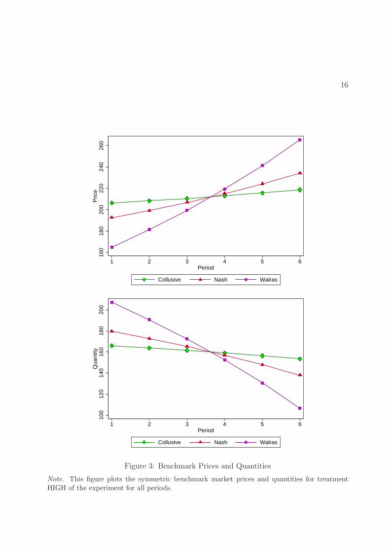
equilibrium numerically using a recursive procedure.12 Figure 3 shows the benchmark

price and quantity levels for one of the parameter combinations used in the experiment

(for treatment HIGH). The figure shows that prices are increasing at the highest rate in

the Walras benchmark and at the lowest rate in the Collusive benchmark. This implies

that p0 is lowest for the Walras benchmark and highest for the Collusive benchmark.13

It is important to note that for figure 3 we assumed that producers stick to each

benchmark perfectly. However, both in the experiment and in real life it is possible that

producers make mistakes or switch between benchmarks after period 1. To allow for

these possibilities, we also calculated the Nash, Collusive and Walras strategies for every

possible state of the market (i.e. every possible period/stock combination); these are the

12In the terminology of Basar and Olsder, 1999, we are solving for the feedback Nash equilibrium.Since the producer problem in the experiment is a ladder-nested multi-act feedback game, the numericalprocedure we use for the feedback Nash equilibrium is the one described by Basar and Olsder (1999) onpage 119-121.

13Since high prices and low production levels go together, collusion actually leads to slower extractionand greater conservation of the resource. This point was also noted by Solow, 1974, who argued that “ifa conservationist is someone who would like to see resources conserved beyond the pace that competitionwould adopt, then the monopolist is the conservationists friend. No doubt they would both be surprisedto know it.” (Solow, 1974, p. 5)

15

benchmarks we compare our results to in the results section.

Finally, in what follows we will sometimes refer to unconstrained or static benchmarks.

The unconstrained benchmark quantities are the quantities that would be adopted in the

absence of resource scarcity; the market quantities Qt are equal toN

N+1

ab, 1

2

aband a

bfor Nash,

Collusion and Walras respectively. From equation 1 it is easy to see that unconstrained

benchmarks always encompass larger production levels (and thus lower prices) than their

dynamic counterparts.

4 Hypotheses

In previous sections we saw that the Hotelling rule does not seem to describe the data very

well. In this paper, we argue that the failure of the Hotelling rule may be the result of

the multifacetedness of the Hotelling framework. Indeed the nonrenewable resource prob-

lem is a mixture of several aspects, including for example exploration, strategic behavior,

technological developments, dynamic optimization etc. Moreover, we argue that resource

owners do not always take every aspect fully into account in their decision making process.

In this section, we will examine this line of reasoning in greater detail and relate it to the

hypotheses that are tested in the experiment.

One reason why producers do not take all aspects fully into account simultaneously is

that doing so may be computationally impossible. Indeed, despite the enormous financial

capabilities of some nonrenewable resource producers, even a very rich nonrenewable re-

source owner may not have a large enough computational capacity to take every aspect

into account for all future periods. Pindyck (1981) argues that having a limited compu-

tational capacity may induce producers to (partially) ignore the dynamic consequences of

their extraction decision. In general, including more than two aspects into a Hotelling

framework may make the optimization problem intractable. Thus, resource owners have

16

160

180

200

220

240

260

Pric

e

1 2 3 4 5 6Period

Collusive Nash Walras

100

120

140

160

180

200

Qua

ntity

1 2 3 4 5 6Period

Collusive Nash Walras

Figure 3: Benchmark Prices and Quantities

Note. This figure plots the symmetric benchmark market prices and quantities for treatmentHIGH of the experiment for all periods.

17

to make choices on what aspects of the decision problem they are going to focus their

computational resources.

Secondly, even if a producer did have the ability to include every aspect of the nonre-

newable resource problem in its decision making process, it might not be beneficial for her

to do so from a cost-benefit perspective. For example, computing the dynamically optimal

time path would require a knowledge of future demand elasticities. However, making accu-

rate predictions about future demand elasticities is likely to be quite costly. An accurate

prediction would for example require incorporating the expected availability of a backstop

technology in the future, the expected sensitivity of consumers to environmental issues,

expected population growth etc. At the same time, even a sizable change in the expected

demand elasticity in 15 or 20 years may not affect the optimal current extraction rate very

much. Indeed, for a resource stock that will not be depleted for many decades, even ignor-

ing the resource constraint completely may not lead to a very different time path in the

short run, since initial production levels may already be quite close to the unconstrained

level. Thus, if fully incorporating certain aspects of the resource problem is costly and the

benefits of doing so are small at least in the short run, then incorporating these aspects

into the decision process may not be worth the costs.

Thirdly, not all aspects of the nonrenewable resource problem may be equally salient to

a producer. For example, the manager of an oil firm with a substantial remaining resource

pool -particularly one who expects to retire or move jobs in the not too distant future- may

not be very mindful of finding a dynamically optimal production strategy. Indeed, doing

so will be beneficial for the company in the long run only and may even reduce profits

in the short run. As Cairns (1986) and Slade (1988) have argued, this means that in

practice the concerns of mining firms are likely to be dominated by price volatility, capital

accumulation or cost control rather than dynamic optimization. Similarly, resource state

companies might be under pressure from their government to acquire immediate income to

18

finance public spending (see e.g. Ezzati, 1976; Teece, 1982; Griffin, 1985). Since the goal of

increasing short term revenue is likely to be in direct conflict with maximizing long term

profits, this will also lead the producer off the dynamically optimal path.14

Thus, the degree to which a nonrenewable resource producer pays attention to a given

aspect of the resource problem depends on whether it can be feasibly included in the op-

timization problem, whether the benefits of including it outweigh the costs and whether

the aspect is salient to the producer. In this article, we focus on what we have previously

argued are two of the most important aspects of the nonrenewable resource problem: dy-

namic optimization and strategic behavior.15 Here, the dynamic optimization aspect refers

to the ability to allocate resource production over time in a dynamically efficient way,

whereas the strategic behavior aspect refers to the ability to base a production strategy

on the expected production strategy of other producers. Moreover, we propose that the

degree to which producers focus on either dynamic optimization or strategic behavior is a

function of the size of the remaining private resource stock.

We experimentally induced variation in stock size by running two treatments of a

non-renewable resource duopoly along the lines of the previous section (with N equal to

2). In treatment LOW, the unconstrained collusive quantity -which is the lowest of the

three unconstrained benchmarks- could be maintained for only one period. In treatment

HIGH, firms had a larger stock; as a result the unconstrained collusive benchmark could be

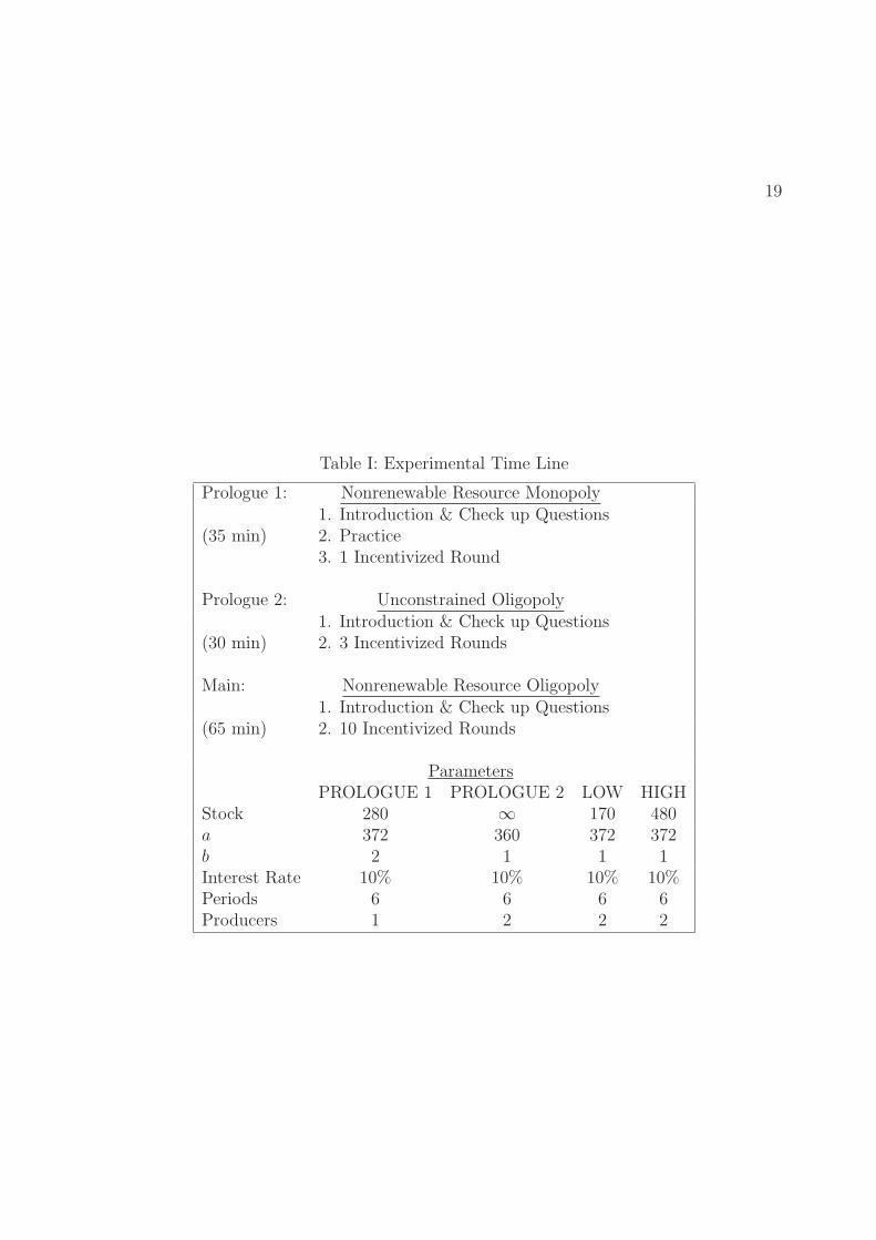
maintained for up to five periods. Table I gives an overview of the parameters corresponding

to the three treatments.16

14An interesting example is provided by the island republic of Nauru. The surface of the island ofNauru consisted almost entirely of phosphate, a nonrenewable resource used to produce fertilizer. Inthe late 60s and early 70s, phosphate production had made Nauru so rich that as a country it had thehighest GDP per capita in the world. However, its government used the proceeds to finance lavish publicspending which eventually led to bankruptcy when the phosphate income started to fall in the 1990s (seee.g. Cox and Kennedy, 2005).

15Although the rest of the article will focus on these two aspects, we do believe that the subsequentanalysis also extends to other aspects.

16Besides stock there were two other parameters which differed between treatments. These were fixedcosts and the conversion rate of experimental points to Euros. They were changed to create similar

19

Table I: Experimental Time Line

Prologue 1: Nonrenewable Resource Monopoly1. Introduction & Check up Questions

(35 min) 2. Practice3. 1 Incentivized Round

Prologue 2: Unconstrained Oligopoly1. Introduction & Check up Questions

(30 min) 2. 3 Incentivized Rounds

Main: Nonrenewable Resource Oligopoly1. Introduction & Check up Questions

(65 min) 2. 10 Incentivized Rounds

ParametersPROLOGUE 1 PROLOGUE 2 LOW HIGH

Stock 280 ∞ 170 480a 372 360 372 372b 2 1 1 1Interest Rate 10% 10% 10% 10%Periods 6 6 6 6Producers 1 2 2 2

20

We propose that the experimentally induced variation in stock size results in a shift of

relative focus between strategic behavior and dynamic optimization. We assume that pro-

ducers in both treatments are computationally constrained, so that they cannot fully take

both aspects into account. Moreover, we assume that the dynamic optimization aspect is

both more salient and more cost-beneficial in treatment HIGH than in treatment LOW.17

In other words, we argue that producers in treatment HIGH will pay less attention to dy-

namic optimization than producers in treatment LOW; conversely producers in treatment

HIGH will pay more attention to strategic behavior.

To test this idea we estimate producers’ production functions by means of a panel

regression. With regard to the dynamic optimization aspect, a dynamically optimized

strategy requires the extraction decision to be a function of the remaining resource stock.

In terms of the estimated production function, producers who take dynamic optimization

into account should -all other things being equal- extract a larger quantity of resources

for higher levels of their resource stock. To the extent that producers in treatment HIGH

pay less attention to dynamic optimization, these producers should then be less likely to

condition their production decision on their remaining resource stock. This leads to the

following hypothesis:

Hypothesis 1A: Producers in treatment HIGH condition their production decision less

strongly on their own stock than producers in treatment LOW.

With regard to the strategic behavior aspect, a dual line of reasoning holds. In partic-

ular, for producers who behave strategically the extraction decision should be a function

of the expected production level of the other producer on the market. To the extent that

producers in treatment HIGH pay more attention to strategic behavior, we expect firms in

incentives in all treatments; they did not affect any of the benchmarks in any way.17Relative to the static Nash level, producing according to the dynamic Nash level yields a 61% higher

revenue for treatment LOW compared to a 48% higher revenue in treatment HIGH.

21

treatment HIGH to be more likely to base their production decision on the expected pro-

duction level of the other producer on the market. This leads to the following hypothesis:

Hypothesis 1B: Producers in treatment HIGH condition their production decision more

strongly the expected production level of the other producer than producers in treat-

ment LOW.

If producers in treatment HIGH indeed focus less on the dynamic optimization aspect

than producers in treatment LOW, this should also be visible in market production levels.

In particular, a producer who pays no heed to the dynamic optimization aspect cannot

produce according to a dynamic benchmark. Instead, the only available alternative is

to produce according to an unconstrained benchmark. Since unconstrained benchmarks

have a higher extraction rate than their dynamic counterparts, producers who adopt an

unconstrained benchmark will push up average production levels away from the Nash level.

This will also pull down prices and scarcity rents, leading to a failure of the Hotelling rule.

All in all, to the extent that producers in treatment HIGH are more likely to produce

according to a static benchmark, production levels should be further away from the Nash

benchmark in treatment HIGH. This leads to the following hypothesis:

Hypothesis 2: Producers in treatment HIGH are more likely to overproduce relative to

the Nash benchmark than producers in treatment LOW.

5 Experimental Design

The experiment was computerized using PhP/MySQL and consisted of two stages: the

prologue and the main part (see table I). We realized that the nonrenewable resource

22

problem would initially be difficult for many participants to tackle. Since we did not want

the Hotelling rule to fail because of a lack of understanding, we instituted a prologue

that helped participants get to know the nonrenewable resource oligopoly problem in a

stepwise way. The first phase of the prologue familiarized participants with the dynamic

optimization aspect and the second phase familiarized them with strategic behavior. All

in all, the prologue lasted for approximately 65 minutes.18 The prologue was identical for

both treatments; treatment variation took place in the main part only. The main part

consisted of a nonrenewable resource duopoly; it will be the focus of the analysis in the

next section. It lasted for approximately 65 minutes as well, bringing the total duration of

the experiment to 2 hours and 30 minutes including a questionnaire and payment.

The first phase of the prologue consisted of a nonrenewable resource monopoly. Partic-

ipants first received a set of instructions and check-up questions (all instructions, questions

and questionnaires are reprinted in appendix B). Once every participant had finished these,

the experiment moved to a 15 minute practice stage. In this practice stage each participant

represented a resource owner with a limited stock of resources to be allocated over a total

of 6 time periods, along the lines of the model of section 3 with N = 1. Thus, participants

were monopolists, which allowed them to learn about the the dynamic optimization aspect

without having to worry about strategic behavior. In every time period, each participant

decided how much of her resource to extract in the current period and how much to save

for the remainder. After making a decision, the participant moved on to the next period

where she again had to decide how much of her resource to extract. The resulting deci-

sion problem is non-trivial because of discounting;19 we incorporated discounting into the

experiment by explicitly introducing an interest rate, such that income earned in earlier

18As a bonus, the prologue also allowed us to compare behavior in the prologue to behavior in the mainpart of the experiment.

19Without discounting, all three benchmarks would collapse into extracting one sixth of the stock inevery period.

23

periods would be worth more.20

After the sixth and final time period, participants were informed of their total income,

which was calculated by adding profits and interest incomes from all periods and subtract-

ing a fixed cost. This ended the first practice round; participants could then immediately

proceed to the next practice round. During practice time participants could go through as

many practice rounds of the monopoly set-up as they liked.21 Thus, each participant had

the time to check many possible production paths; as a result we expected most to get to

know at least the basic rule of dynamic optimization in a nonrenewable resource context

-which is to produce more in early periods than at the end. To make sure that every par-

ticipant put in sufficient effort during practice, we also included a fully incentived round

after practice. All in all, the first phase of the prologue took approximately 35 minutes.

The next phase of the prologue consisted of an unconstrained duopoly. As a result,

phase two allowed participants to familiarize themselves with the presence of another pro-

ducer on the market (the strategic behavior aspect) without having to worry about dynamic

optimization. In particular, we expected that phase two would teach participants at least

the basic rule of Cournot oligopoly -which is that (up to a point) increasing production

in a given period will increase your profits, but decrease the profits of the other producer

on the market. Like phase one, phase two started off with a new set of instructions and

questions. Participants then went through three rounds of the unconstrained oligopoly

set-up; in every round participants were matched with one other participant, so that there

were always two active producers on every market. Each round consisted of six periods

as in the previous phase of the prologue; each market moved on to the next period once

20A possible alternative sometimes used in the literature is to use a stochastic ending mechanism.However, explicitly incorporating an interest rate avoids issues of risk aversion, the gambler’s fallacy (seee.g. Terrel, 1994) and keeps all rounds comparable (same number of periods), whilst also staying close tothe theoretical framework. In any case, Brown, Flinn, and Schotter (2011) show that both mechanismsmay yield very similar results.

21On average, participant went through 26 practice rounds, with a minimum of 10 and a maximum of53.

24

both producers had made their production decision. The experiment then moved forward

towards the next round once all markets had finished all six periods; all three rounds con-

tributed to final earnings. In total, phase two of the prologue lasted approximately 30

minutes.

After everyone had finished the prologue, the experiment moved on to the main part,

which forms the basis for the analysis presented in the next section. All participants

received a final set of instructions and questions and then went through ten incentivized

rounds of the nonrenewable resource oligopoly framework of section 3. The main part thus

incorporated both the dynamic optimization aspect and the strategic behavior aspect. Each

participant represented a resource owner with a limited stock of resources (as in the first

phase of the prologue); moreover participants were paired so that there were always two

active producers on every experimental market (as in the second phase of the prologue).

During the decision process the decision screen gave participants access to the pro-

duction decisions of both participants as well as the price levels in preceding periods and

remaining resource stocks.22 After the sixth and final time period, participants were in-

formed of their total income, which was calculated by adding profits and interest incomes

from all periods and subtracting a fixed cost. Once all other pairs were done as well, the

experiment moved on to the next round, where the same set-up was repeated. In every

round, participants were matched to a different participant in their matching group.23 In

total, there were ten rounds, each of which was incentivized.

In general, we realized that the decision problem would be quite hard for many par-

ticipants for a large time horizon or a large number of competitors, even after having

familiarized them with both aspects of the nonrenewable resource problem in the prologue.

22An example of a decision screen is given at the end of Appendix B.23Matching groups consisted of between 6 and 10 participants, depending on the number of participants

in the session. Participants could only be matched to participants from their matching group. Moreover,participants could never face the same participant twice in succession. Finally, participants never learnedthe identity of the other participant.

25

Hence, we stuck to a relatively simple set-up by limiting the number of periods to six and

market size to two firms.24 Moreover, all participants had access to an on-screen calculator

which allowed them to compute the profits and interest incomes for any period and any

production level of themselves and the other producer.

One final thing to note about the main part is that in every even round participants were

asked in every period to indicate to predict how much the other firm to produce in that

period. Any strategic production decision directly depends on the expected production

strategy of other producers; a big advantage of experiments is that expectations can be

elicited directly.25 Predictions were incentivized; at the end of the experiment, participants

received a payment depending on the accuracy of one randomly determined prediction.

For this purpose, we asked one subject to come forward and roll a die to determine the

prediction round and period that would be used to determine payment. Prediction income

was then computed using a linear scoring rule, where a unit deviation from the actual value

would reduce earnings by 20 cents, from a maximum of five to a minimum of zero Euros.

After finishing the last round of the main part, participants received an overview of

their earnings over the whole experiment. They were then asked to fill out a questionnaire,

which consisted of some background questions, some questions relating to the way they

played in the experiment as well as the shortened version of the Stanford Time Perspective

Inventory (D’Alessio et al., 2003) -a questionnaire related to time preferences.

24Indeed, we had previously run a pilot (Van Veldhuizen, 2009) where we had 10 periods and a groupsize of three and found that a small number of participants occasionally took a very long time (sometimesnearly 10 minutes) to make a single production decision. Since 98% of all decisions in the pilot were madewithin 90 seconds, we decided to limit the decision time per period to two minutes.

25However, elicited expectations are not uncontroversial in the literature. In particular, they mightsuffer from a false consensus or reciprocity effect (see e.g. Croson, 2000) and even the elicitation procedureitself may change behavior in a round (see e.g. Gachter and Renner, 2010). We come back to this issue inappendix A.

26

6 Results

The experiment was conducted in February 2010 at the CREED laboratory of the Uni-

versity of Amsterdam. Participants were recruited using an online registration system.

Most participants were students coming from various disciplines, with the largest fraction

(58%) studying economics. In total, there were 6 sessions (3 for treatment HIGH and 3

for treatment LOW) in which a total of 136 subjects took part (72 for treatment HIGH,

64 for treatment LOW). On average, participants earned 29.27 euros.

In this section, we first take a brief look at the results of the prologue to check if

participants were able to independently understand both strategic behavior and dynamic

optimization. We then estimate their production function to gain insight into which aspect

producers paid most attention to when making their production decision. The next sub-

section then brings together the prologue and the main part as a second way to investigate

what aspect producers paid most attention to. Finally, we examine if differences in the

production function are reflected by market outcomes as well.

6.1 Prologue

The purpose of the first phase of the prologue (monopoly) was to familiarize participants

with the dynamic optimization aspect of the nonrenewable resource problem. In partic-

ular, we expected participants to learn at least the basic rule of dynamic optimization,

which dictates that scarcity rents should be monotonically nondecreasing over time. This

expectation is supported by the data: scarcity rents were nondecreasing for 90% of our

participants (or 123/136). Moreover, 89% (121/136) displayed a significant positive time

trend in scarcity rents.26 Furthermore, 87% (118/136) exceeded the earnings corresponding

26The trend was estimated using a linear regression of scarcity rent on a constant and a linear timetrend; significance was obtained using a two-sided t-test with a significance level of 5%.

27

7080

9010

011

012

0S

carc

ity R

ent

1 2 3 4 5 6Period

Observed Optimal

01

23

4D

ensi

ty

−1 −.5 0 .5 1Scarcity Rent

Figure 4: Monopoly

Notes. The top panel of the figure plots the time series of the average observed scarcity rent and theoptimal scarcity rent conditional on the average remaining resource stock. The lower panel plots the

smoothed density of the deviation from the optimal scarcity rent divided by the optimal quantityλt−λo

t

qot

(Epanechnikov kernel, bandwidth = .028). We use deviations from the optimal scarcity rent since theoptimal scarcity rent differs depending on the period and the remaining resource stock. Deviations areweighted by the optimal quantity to take into account that a unit deviation from the optimum should begiven more weight in periods where the expected optimal production is already quite low.

28

200

250

300

350

Qua

ntity

1 2 3 4 5 6Period

Observed Quantity CollusiveNash Walras

0.0

05.0

1.0

15.0

2.0

25D

ensi

ty

0 60 120 C N 300 WMarket Quantity

0.0

1.0

2.0

3.0

4.0

5D

ensi

ty

0 30 60 C N 150 WProducer Quantity

Figure 5: Unconstrained Oligopoly

Notes. The top panel of the figure plots the time series of the average observed market quantities as wellas the three benchmarks. The middle and lower panels plot the smoothed density of observed market(Epanechnikov kernel, bandwidth = 4) and individual quantities (bandwidth=2) over all periods respec-tively. C, N and W represent the Cournot, Nash and Walras quantities.

29

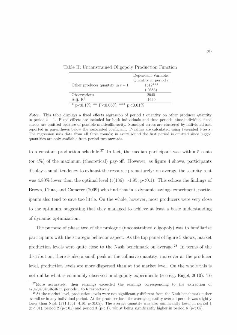
Table II: Unconstrained Oligopoly Production Function

Dependent Variable:Quantity in period t

Other producer quantity in t− 1 .1512***(.0386)

Observations 2040Adj. R2 .1640

* p<0.1%; ** P<0.05%; *** p<0.01%

Notes. This table displays a fixed effects regression of period t quantity on other producer quantityin period t − 1. Fixed effects are included for both individuals and time periods; time-individual fixedeffects are omitted because of possible multicollinearity. Standard errors are clustered by individual andreported in parentheses below the associated coefficient. P-values are calculated using two-sided t-tests.The regression uses data from all three rounds; in every round the first period is omitted since laggedquantities are only available from period two onwards.

to a constant production schedule.27 In fact, the median participant was within 5 cents

(or 4%) of the maximum (theoretical) pay-off. However, as figure 4 shows, participants

display a small tendency to exhaust the resource prematurely: on average the scarcity rent

was 4.80% lower than the optimal level (t(136)=-1.95, p<0.1). This echoes the findings of

Brown, Chua, and Camerer (2009) who find that in a dynamic savings experiment, partic-

ipants also tend to save too little. On the whole, however, most producers were very close

to the optimum, suggesting that they managed to achieve at least a basic understanding

of dynamic optimization.

The purpose of phase two of the prologue (unconstrained oligopoly) was to familiarize

participants with the strategic behavior aspect. As the top panel of figure 5 shows, market

production levels were quite close to the Nash benchmark on average.28 In terms of the

distribution, there is also a small peak at the collusive quantity; moreover at the producer

level, production levels are more dispersed than at the market level. On the whole this is

not unlike what is commonly observed in oligopoly experiments (see e.g. Engel, 2010). To

27More accurately, their earnings exceeded the earnings corresponding to the extraction of47,47,47,47,46,46 in periods 1 to 6 respectively.

28At the market level, production levels were not significantly different from the Nash benchmark eitheroverall or in any individual period. At the producer level the average quantity over all periods was slightlylower than Nash (F(1,135)=4.10, p<0.05). The average quantity was also significantly lower in period 1(p<.01), period 2 (p<.01) and period 3 (p<.1), whilst being significantly higher in period 6 (p<.05).

30

check if participants understood the strategic behavior aspect, we use a panel regression

to estimate their production function. Producers display evidence of strategic behavior if

they condition their production strategy on the expected production strategy of the other

producer. Since we did not elicit expectations in the prologue, we proxy for expectations

using last period’s other producer quantity.29 Table II documents the results of the regres-

sion. On average, participants increased their production if their rival previously produced

a high quantity. All in all, the finding that average production levels are close to the

Nash level and that participants production decisions are correlated to last period’s other

producer quantity suggest that most participants also gained some understanding of the

strategic behavior aspect.

6.2 Producer Focus in the Main Part

We now turn to producer focus in the main part, where both strategic behavior and dy-

namic optimization were possible. We investigate the degree to which producers pay atten-

tion to either dynamic optimization or strategic behavior by estimating their production

function. For this purpose we estimate the following panel regression:

qrit = β ∗ E[qrjt] + γ1 ∗ Srit + γ2 ∗ Srjt + Tt + δi + ǫrit (3)

This equation posits that producer i’s quantity in period t of round r is a function of both

strategic and dynamic optimization variables. E[qrjt] is producer i’s prediction for the

quantity of producer j (the other producer); this variable represents the degree to which

producer i pays attention to the strategic behavior aspect.30 Srit is the producer i’s stock,

29This is a good proxy to the extent that participants based their expectations on what the other firmproduced in the previous period. See appendix A for evidence that suggests that this is indeed the case.

30Since producers were asked to make predictions and production decisions simultaneously, there arelegit concerns that predictions may be endogenous. This issue is addressed in appendix A both usingan Instrumental Variables approach and using lagged other producer quantity as an indirect measure ofexpectations.

31

which represents the dynamic optimization aspect. Srjt is the other producer’s stock; this

variable is relevant only if both dynamic optimization and strategic behavior play a role,

as in the dynamic Nash benchmark. Finally, the regression also includes time fixed effects

(Tt) and individual fixed effects (δi) to correct for differences between people and periods.31

Throughout the analysis, standard errors are clustered by producer.32 Note also that the

inclusion of the prediction variable means that the analysis will only use data from rounds

where predictions were requested (i.e. all even rounds).33

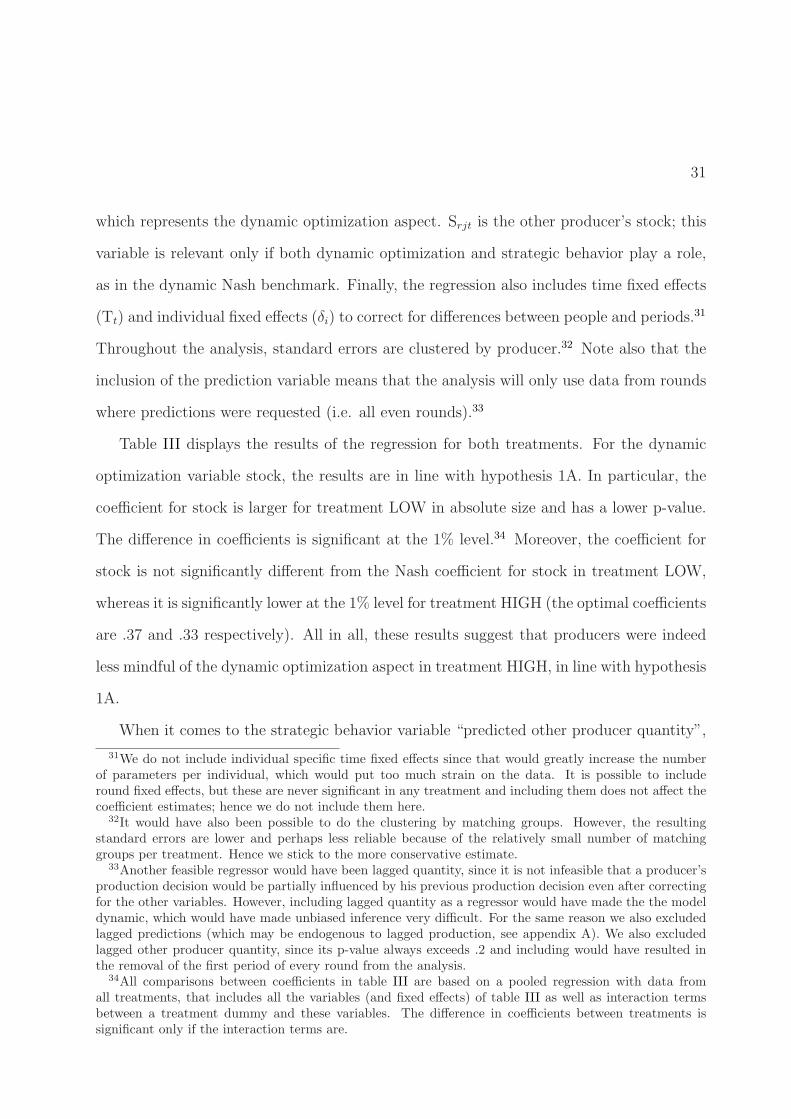
Table III displays the results of the regression for both treatments. For the dynamic

optimization variable stock, the results are in line with hypothesis 1A. In particular, the

coefficient for stock is larger for treatment LOW in absolute size and has a lower p-value.

The difference in coefficients is significant at the 1% level.34 Moreover, the coefficient for

stock is not significantly different from the Nash coefficient for stock in treatment LOW,

whereas it is significantly lower at the 1% level for treatment HIGH (the optimal coefficients

are .37 and .33 respectively). All in all, these results suggest that producers were indeed

less mindful of the dynamic optimization aspect in treatment HIGH, in line with hypothesis

1A.

When it comes to the strategic behavior variable “predicted other producer quantity”,

31We do not include individual specific time fixed effects since that would greatly increase the numberof parameters per individual, which would put too much strain on the data. It is possible to includeround fixed effects, but these are never significant in any treatment and including them does not affect thecoefficient estimates; hence we do not include them here.

32It would have also been possible to do the clustering by matching groups. However, the resultingstandard errors are lower and perhaps less reliable because of the relatively small number of matchinggroups per treatment. Hence we stick to the more conservative estimate.

33Another feasible regressor would have been lagged quantity, since it is not infeasible that a producer’sproduction decision would be partially influenced by his previous production decision even after correctingfor the other variables. However, including lagged quantity as a regressor would have made the the modeldynamic, which would have made unbiased inference very difficult. For the same reason we also excludedlagged predictions (which may be endogenous to lagged production, see appendix A). We also excludedlagged other producer quantity, since its p-value always exceeds .2 and including would have resulted inthe removal of the first period of every round from the analysis.

34All comparisons between coefficients in table III are based on a pooled regression with data fromall treatments, that includes all the variables (and fixed effects) of table III as well as interaction termsbetween a treatment dummy and these variables. The difference in coefficients between treatments issignificant only if the interaction terms are.

32

Table III: Main Part Production Function

Dependent Variable: QuantityLOW HIGH

Coeff. Std Err. Coeff. Std Err.Predicted other producer quantity .3050*** .0809 .3340*** .0632Stock .4269*** .0422 .1890*** .0629Other producer stock -.0884*** .0250 -.0189 .0157Observations 1600 1800Adj. R2 .7436 .4766

* significant at 10%; ** significant at 5%; *** significant at 1%

Notes. This table contains the results of a panel regression of quantity on the predicted quantity of theother producer, stock and the stock of the other producer. Period and producer fixed effects are alsoincluded but not reported; standard errors are clustered at the producer level. Predictions were onlyelicited in even rounds; moreover, the final period is omitted from the analysis since all benchmarks aretrivially equal to the remaining resource stock in the final period. Thus, the number of observations perindividual in all treatments is equal to 25, 5 rounds with 5 observations each. P-values are calculated usingtwo-sided t-tests.

results are less clear cut. On the one hand, the results are in the direction predicted

by hypothesis 1B: a change in predicted other producer quantity had a larger effect in

treatment HIGH than in treatment LOW. On the other hand, the difference between

treatments is small and not significant at conventional levels.35

The final variable -the other producer’s stock- should only be significant for producers

who adopt a dynamic Nash strategy that incorporates both dynamic optimization and

strategic behavior. This variable is significant only in treatment LOW (in the direction

predicted by the Nash benchmark), which suggests that producers in treatment LOW

were more likely to adopt a dynamic Nash strategy. This is in line with the finding that

dynamic optimization behavior appears more strongly in treatment LOW whereas there is

little evidence for differences in the level of strategic behavior.

35We also ran two separate sessions where production in the main part was unconstrained. Repeatingthe regression of table III for these sessions gives a higher coefficient (.3941, with S.E. .0793) for predictedother producer quantity, although the difference in coefficients with treatment LOW and treatment HIGHwas also not significant.

33

6.3 Comparing the Prologue and the Main Part

Thus we have seen that in terms of the production function, the dynamic optimization

aspect seemed to be more important in treatment LOW, whereas there was no pronounced

pattern for the strategic behavior aspect. Another way to examine producer focus in the

main part is to correlate behavior in the main part to behavior in the prologue. Specifi-

cally, if hypotheses 1A and 1B are correct, the degree to which behavior correlates between

the prologue and the main part could also depend on the treatment. Behavior in treat-

ment LOW should then be most correlated to behavior in the monopoly phase of the

prologue, whereas behavior in treatment HIGH should be most correlated to the uncon-

strained oligopoly phase.

To test this idea we regressed indicators of behavior and success in the main part

on similar indicators from the prologue. From the monopoly part of the prologue we

take the difference between the first period scarcity rent and last period scarcity rent (or

dispersion) as an indicator of dynamic optimization. For the unconstrained oligopoly part

of the prologue we take first period production quantity as a measure of the intention to

produce cooperatively. Moreover we take a measure of income in both parts and correlate

that with main part income to see if success is also correlated between the prologue and

the main part.36

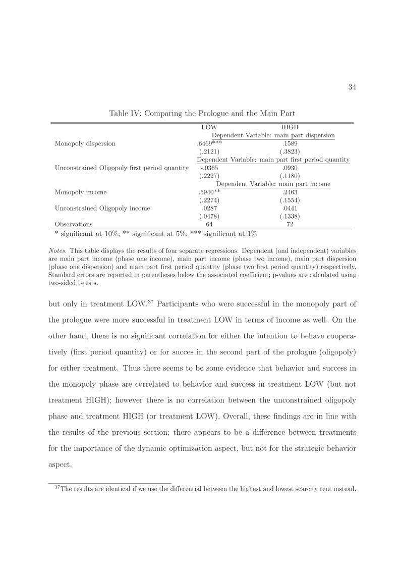
Table IV shows the result of these regressions. Firstly, participants with a high dis-

persion in the monopoly part of the prologue also had a high dispersion in the main part,

36In comparing the unconstrained oligopoly with the main part we correlated overall income in theunconstrained oligopoly to overall income in the main part. However, for the monopoly part there areseveral complications: (a) because of practice almost all participants were able to do well in the monopolypart of the prologue; as a result there was little variation in the production schedule used in the incentivizedround. Moreover, (b) starting from round two participants in the main part could also adopt the productionschedule they learned from the other producer in a preceding round. To solve the first problem, weconstructed a dummy variable which was equal to one only if the participant managed to run a profit inat least one of his first three practice rounds (the results are similar if we take the first four, five or sixpractice rounds instead). This split the sample roughly in half, since 57% of participants managed to runa positive profit in one of the first three practice rounds. To adress possible learning considerations weused only the first round of the main part.

34

Table IV: Comparing the Prologue and the Main Part

LOW HIGHDependent Variable: main part dispersion

Monopoly dispersion .6469*** .1589(.2121) (.3823)Dependent Variable: main part first period quantity

Unconstrained Oligopoly first period quantity -.0365 .0930(.2227) (.1180)

Dependent Variable: main part incomeMonopoly income .5940** .2463

(.2274) (.1554)Unconstrained Oligopoly income .0287 .0441

(.0478) (.1338)Observations 64 72

* significant at 10%; ** significant at 5%; *** significant at 1%

Notes. This table displays the results of four separate regressions. Dependent (and independent) variablesare main part income (phase one income), main part income (phase two income), main part dispersion(phase one dispersion) and main part first period quantity (phase two first period quantity) respectively.Standard errors are reported in parentheses below the associated coefficient; p-values are calculated usingtwo-sided t-tests.

but only in treatment LOW.37 Participants who were successful in the monopoly part of

the prologue were more successful in treatment LOW in terms of income as well. On the

other hand, there is no significant correlation for either the intention to behave coopera-

tively (first period quantity) or for succes in the second part of the prologue (oligopoly)

for either treatment. Thus there seems to be some evidence that behavior and success in

the monopoly phase are correlated to behavior and success in treatment LOW (but not

treatment HIGH); however there is no correlation between the unconstrained oligopoly

phase and treatment HIGH (or treatment LOW). Overall, these findings are in line with

the results of the previous section; there appears to be a difference between treatments

for the importance of the dynamic optimization aspect, but not for the strategic behavior

aspect.

37The results are identical if we use the differential between the highest and lowest scarcity rent instead.

35

100

150

200

250

Sca

rcity

Ren

t

1 2 3 4 5 6Period

Observed CollusiveNash Walras

Figure 6: Treatment LOW Scarcity Rents

Notes. The figure plots the time series of the average observed scarcity rent as well as the benchmarkNash, Collusive and Walras scarcity rent with respect to the unconstrained Nash price. This is equivalentto subtracting a fixed number (pNU = 124) from the observed and benchmark prices respectively (i.e.pi − pNU , where pi is the observed, Nash, Collusive or Walras price respectively). Here we use the dynamicbenchmarks that depend on the current state of the market.

6.4 Market Outcomes in the Main Part

In the previous sections we saw that the dynamic optimization aspect seemed to be less

important in treatment HIGH. If hypothesis 2 is true, producers in treatment HIGH should

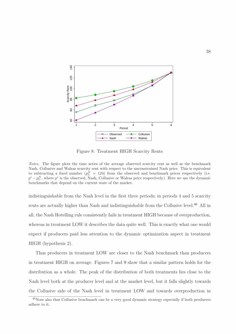
then be more likely to overproduce relative to the Nash benchmark.38 Figures 6 to 9 and

table V give an overview of scarcity rents and production levels in the main part. For

treatment HIGH, average production levels are higher than the Nash level in all periods;

as a result the average scarcity rents are lower.39 For treatment LOW, the scarcity rent is

38It is important to restate that when we refer to the Nash, Walras or Collusive benchmarks in thissection, we refer to the dynamic benchmarks that depend on the current state of the market (i.e. theperiod/stock level combination). In particular, since in a given period, different markets will in generalproduce different quantities, stock levels will differ between markets from period 2 onwards. As a conse-quence, each market will in general have a different Nash, Collusive and Walras benchmarks from period2 onwards as well.

39Since scarcity rents and prices are an affine transformation of market quantities, the test statistics formarket quantities, prices and scarcity rents are identical.

36

0.1

.2.3

.4D

ensi

ty

−4 −3 −2 C N 1 W 3 4Weighted Market Quantity

0.1

.2.3

.4D

ensi

ty

−4 −3 −2 C N 1 W 3 4Weighted Producer Quantity

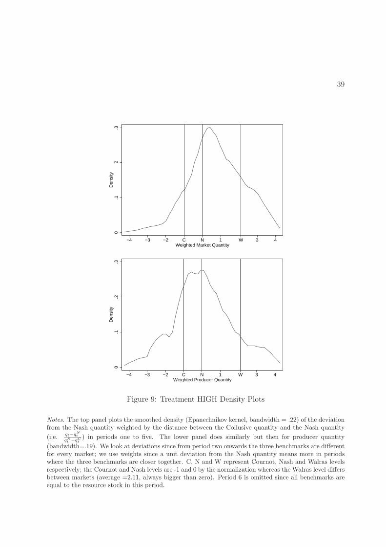
Figure 7: Treatment LOW Density Plots

Notes. The top panel plots the smoothed density (Epanechnikov kernel, bandwidth = .26) of the deviationfrom the Nash quantity weighted by the distance between the Collusive quantity and the Nash quantity

(i.e.qt−qN

t

qNt−qC

t

) in periods one to five. The lower panel does similarly but then for producer quantity

(bandwidth=.28). We look at deviations since from period two onwards the three benchmarks are differentfor every market; we use weights since a unit deviation from the Nash quantity means more in periodswhere the three benchmarks are closer together. C, N and W represent Cournot, Nash and Walras levelsrespectively; the Cournot and Nash levels are -1 and 0 by the normalization whereas the Walras level differsbetween markets (average =1.91, always bigger than zero). Period 6 is omitted since all benchmarks areequal to the resource stock in this period.

37

Table V: Main Part Market Quantity and Benchmarks

Treatment LOW (N=320)Period Average Quantity Nash Collusive Walras

1 101.70 100 85*** 123***(2.192) (2.192) (2.192) (2.192)

2 80.75 83.04 72.70** 102.69***(2.322) (2.691) (2.596) (2.692)

3 64.65 67.23 59.62* 82.32***(1.338) (2.184) (2.149) (2.476)

4 45.975 50.28** 45.31 60.40***(1.149) (1.270) (1.146) (1.595)

5 29.67 32.97*** 30.77* 38.14***(1.924) (.737) (.494) (1.029)

6 17.21 17.27 17.27 17.27(2.646) (.037) (.037) (.037)

Treatment High (N=360)Period Average Quantity Nash Collusive Walras

1 192.22 180*** 166*** 207***(3.686) (3.686) (3.686) (3.686)

2 178.74 168.79*** 159.43*** 193.10***(1.940) (2.448) (2.510) (2.510)

3 170.30 160.44** 152.46*** 178.15**(2.070) (3.138) (3.186) (3.186)

4 158.11 149.40*** 143.71*** 161.13(1.567) (2.004) (2.022) (2.022)

5 141.96 135.46*** 132.63*** 141.49(2.492) (1.318) (1.219) (1.219)

6 117.03 117.97** 117.97** 117.97**(4.571) (.357) (.357) (.357)

* significant at 10%; ** significant at 5%; *** significant at 1%

Notes. This table compares the observed average market quantity per period to the Nash, Collusive andWalras benchmark for every treatment. Here we use the dynamic benchmarks that depend on the currentstate of the market. For this purpose, all three benchmarks are calculated for every data point conditionalon period, producer stock and other producer stock and then summed over both producers on the market.In the first period, all benchmark quantities are integers since all producers have the same resource stockand only integer amounts can be produced. In the final period, fully exhausting the resource is always theoptimal strategy regardless of benchmark and treatment. Standard errors are clustered at the matchinggroup level. Significance is determined using two-sided t-tests.

38

4060

8010

012

014

0S

carc

ity R

ent

1 2 3 4 5 6Period

Observed CollusiveNash Walras

Figure 8: Treatment HIGH Scarcity Rents

Notes. The figure plots the time series of the average observed scarcity rent as well as the benchmarkNash, Collusive and Walras scarcity rent with respect to the unconstrained Nash price. This is equivalentto subtracting a fixed number (pNU = 124) from the observed and benchmark prices respectively (i.e.pi − pNU , where pi is the observed, Nash, Collusive or Walras price respectively). Here we use the dynamicbenchmarks that depend on the current state of the market.

indistinguishable from the Nash level in the first three periods; in periods 4 and 5 scarcity

rents are actually higher than Nash and indistinguishable from the Collusive level.40 All in

all, the Nash Hotelling rule consistently fails in treatment HIGH because of overproduction,

whereas in treatment LOW it describes the data quite well. This is exactly what one would

expect if producers paid less attention to the dynamic optimization aspect in treatment

HIGH (hypothesis 2).

Thus producers in treatment LOW are closer to the Nash benchmark than producers

in treatment HIGH on average. Figures 7 and 9 show that a similar pattern holds for the

distribution as a whole. The peak of the distribution of both treatments lies close to the

Nash level both at the producer level and at the market level, but it falls slightly towards

the Collusive side of the Nash level in treatment LOW and towards overproduction in

40Note also that Collusive benchmark can be a very good dynamic strategy especially if both producersadhere to it.

39

0.1

.2.3

Den

sity

−4 −3 −2 C N 1 W 3 4Weighted Market Quantity

0.1

.2.3

Den

sity

−4 −3 −2 C N 1 W 3 4Weighted Producer Quantity

Figure 9: Treatment HIGH Density Plots

Notes. The top panel plots the smoothed density (Epanechnikov kernel, bandwidth = .22) of the deviationfrom the Nash quantity weighted by the distance between the Collusive quantity and the Nash quantity

(i.e.qt−qN

t

qNt−qC

t

) in periods one to five. The lower panel does similarly but then for producer quantity

(bandwidth=.19). We look at deviations since from period two onwards the three benchmarks are differentfor every market; we use weights since a unit deviation from the Nash quantity means more in periodswhere the three benchmarks are closer together. C, N and W represent Cournot, Nash and Walras levelsrespectively; the Cournot and Nash levels are -1 and 0 by the normalization whereas the Walras level differsbetween markets (average =2.11, always bigger than zero). Period 6 is omitted since all benchmarks areequal to the resource stock in this period.

40

treatment HIGH. In terms of market (producer) production levels, 70.5% (62.4%) of all

production levels are larger than the Nash benchmark in treatment HIGH, whereas the

respective percentages are 28.3% (30.5%) for treatment LOW.

Thus, the evidence so far seems to suggest that -in terms of benchmarks- subjects pro-

duced more aggressively in treatment HIGH. To see if this is also reflected by their earnings,

we compare average realized earnings to potential earnings in the Nash benchmark and

weigh this using the distance between the Nash benchmark and the Collusive benchmark.

This results in the normalized earnings index Ynorm = Y−YN

YC−YN

, where YN is the theoretical

Nash profit, YC is the theoretical Collusive profit and Y is actual income.41 The average

index is equal to -6.70 for treatment HIGH and -1.72 for treatment LOW, the difference

is significant at the 1% level (Mann-Whitney, z(64,72)=6.422). In other words, in terms

of the index earnings were significantly lower in treatment HIGH. This is in line with the

finding that producers were more likely to overproduce with respect to Nash in treatment

HIGH.42

In summary, we have seen that producers paid more attention to the dynamic opti-

mization aspect in treatment LOW and that this induced them to produce closer to the

Nash benchmark than producers in treatment HIGH. At the same time, it is worthwhile

to point out that on average producer behavior was quite close to the Nash level in both

treatments. As a result, scarcity rents are actually increasing in both treatments, in line

with the Hotelling rule and contrary to the findings of most previous empirical studies. Im-

portantly, however, producers in treatment HIGH deviate most from the Nash benchmark

and do so in the direction predicted by hypothesis 2. Thus, even producers who -based

41It is not possible to compare realized earnings levels directly because of difference in stock levels, fixedcosts and conversion rates.

42Interestingly, average earnings were below the Nash level in both treatment HIGH and treatmentLOW, despite the finding that in treatment LOW average scarcity rents were never significantly belowthe Nash level. A likely explanation is that although on average the Nash scarcity rent was quite wellapproximated by the data, many individual producers still overproduced or underproduced, which resultedin lower earnings. This idea is supported by the right and lower panels of figures 6 and 8, which showssubstantial heterogeneity in observed production levels.

41

on the evidence of treatment LOW- should be able to approximate the Nash time path

almost perfectly still overproduce if their stock levels are relatively high.

7 Conclusion

The most important theoretical result in the field of nonrenewable resource economics is

the Hotelling rule, which states that scarcity rents should increase over time at the rate of

interest. However, the Hotelling rule has received little empirical support. In this study, we

propose that the failure of the Hotelling rule can be explained by the multifacetedness of the

Hotelling framework. We argue that the nonrenewable resource problem consists of many

different aspects (e.g. exploration, strategic behavior, technological developments, dynamic

optimization etc.) and that in practice, producers may not be willing or able to take every

aspect fully into account. Moreover we argue that the degree to which a nonrenewable

resource producer pays attention to a given aspect of the resource problem depends on the

size or longevity of her resource stock. In particular, we argue that for a relatively scarce

resource it pays off for producers to compute a dynamically optimal production path.

However, for a more abundant resource, computing a dynamically optimal production

path may be infeasible, non-salient or suboptimal from a cost-benefit perspective. Indeed,

we argue that producers with a relatively large stock should focus more on other aspects

of the decision problem, such as strategic behavior. These producers will then (partially)

ignore the dynamic consequences of their extraction decision, which results in suboptimally

low prices and the failure of the Hotelling rule.

This argument is supported by the results of a nonrenewable resource duopoly experi-

ment. In a treatment where resources are relatively scarce (treatment LOW), producers put

more weight on dynamic optimization variables in their production function compared to a

treatment where resources are relatively abundant (treatment HIGH). Similarly, behavior

42

and earnings in treatment LOW are correlated to behavior and earnings in a preceding part

of the experiment where only dynamic optimization is relevant; for treatment HIGH there

is no such correlation. At the same time, there is little evidence that suggests that pro-

ducers pay less attention to strategic behavior in treatment HIGH. The differences in the

estimated production function are reflected by market outcomes, however. In treatment

HIGH, scarcity rents are persistently lower than the Nash level because producers focus

less on dynamic optimization, making them produce closer to the unconstrained levels. On

the other hand, in treatment LOW scarcity rents are very close to the Nash level.

In terms of real world markets, the relative abundance of many non-renewable resources

may have induced producers to overextract, leading to the failure of the Hotelling rule. At

the same time, we do not believe that this is the whole story; indeed in the experiment

scarcity rents are still increasing over time in both treatments. A full explanation of

the failure of the Hotelling rule may also require other elements, including for example

the discovery of new deposits, capacity constraints or technological progress. In future

work, it could be worthwhile to use the experimental approach to try to disentangle the

relative explanatory power of these elements. Indeed, we believe that experimental data

can serve as a complement to field data to aid the profession in gaining a better grasp of

the mechanisms driving the behavior of producers on nonrenewable resource markets.

References

Abbink, K. and J. Brandts. 2008. “Pricing in Bertrand Competition with Increasing

Marginal Costs.” Games and Economic Behavior 63 (1):1–31.

———. 2009. “Collusion in Growing and Shrinking Markets: Empirical Evidence from Ex-

perimental Duopolies;.” In Experiments and Competition Policy, edited by J. Hinloopen

and H.-T. Normann. Cambridge University Press, 34–60.

43

Adelman, M.A. 2002. “World Oil Production and Prices 1947-2000.” The Quarterly Review

of Economics and Finance 42:169–91.

Arrow, K. J. and S. Chang. 1978. “Optimal Pricing, Use and Exploration of Uncer-

tain Natural Resource Stocks.” Journal of Environmental Economics and Management

9 (1):1–10.

Basar, T. and G.J. Olsder. 1999. Dynamic Noncooperative Game Theory. Philadelphia:

Society for Industrial and Applied Mathematics.

BP, British Petroleum. 2010. “British Petroleum Statistical Review 2010.” Available from

http://www.bp.com/ (accessed August 24th, 2010).

Brown, A.L., Z.E. Chua, and C.F. Camerer. 2009. “Learning and Visceral Temptation in

Dynamic Savings Experiments.” Quarterly Journal of Economics 124 (1):197–231.

Brown, M., C.J. Flinn, and A. Schotter. 2011. “Real-Time Search in the Laboratory and

the Market.” American Economic Review 101 (2):948–57.

Bulletin, Energy. 2006. “Clinton: not briefed on peak oil.”

http://www.energybulletin.net/node/18138 (accessed December 14th, 2010).

Cairns, R.D. 1986. “More on Depletion in the Nickel Industry.” Journal of Environmental

Economics and Management 13:93–8.

Cairns, R.D. and G.A. Davis. 1998. “On Using Current Information to Value Hard-Rock

Mineral Properties.” The Review of Economics and Statistics 80 (4):123–40.

Chermak, J.M. and K. Krause. 2002. “Individual Response, Information, and Intergenera-

tional Common Pool Problems.” Journal of Environmental Economics and Management

43:47–70.

44

Cox, J. and J. Kennedy. 2005. “How Much More Rent Could Have Been Extracted From

Nauru’s Phosphate Deposits?” In MODSIM 2005 International Congress on Modelling

and Simulation, edited by A. Zerger and R.M. Argent. Modelling and Simulation Society

of Australia and New Zealand, 170–6.

Croson, R. 2000. “Thinking like a Game Theorist: Factors Affecting the Frequency of

Equilibrium Play.” Journal of Economic Behavior and Organization 41:299–314.

D’Alessio, M., A. Gurarion, V. De Pascalis, and P.G. Zimbardo. 2003. “Testing Zimbardo’s

Stanford Time Perspective Inventory (STPI) -Short Form: An Italian Study.” Time and

Society 12:333–47.

Deffeyes, K. S. 2005. Beyond Oil: The View from Hubbert’s Peak. New York: Hill and

Wang.

Dery, P. and B. Anderson. 2007. “Peak Phosphorus.”

http://www.energybulletin.net/node/33164 (accessed December 14th, 2010).

Devarajan, S. and A.C. Fisher. 1981. “Hotelling’s Economics of Exhaustible Resources:

Fifty Years Later.” Journal of Economic Literature 19 (1):65–73.

Engel, C. 2010. “How Much Collustion? A Meta-Analysis of Oligopoly Experiments.”

Journal of Competition Law and Economics 3 (4):491–549.

Ezzati, A. 1976. “Future OPEC Price and Production Strategies as Affected by its Capacity

to Absorb Oil Revenues.” European Economic Review 8 (2):107–138.

Farrow, S. 1985. “Testing the Efficiency of Extraction from a Stock Resource.” Journal of

Political Economy 93 (3):452–87.

45

Fischer, M.E., B. Irlenbusch, and A. Sadrieh. 2004. “An Intergenerational Common Pool

Resource Experiment.” Journal of Environmental Economics and Management 48:811–

36.

Gachter, S. and E. Renner. 2010. “The Effects of (Incentivized) Belief Elicitation in Public

Good Experiments.” Experimental Economics 13 (3):364–77.

Gaudet, G. 2007. “Natural Resource Economics under the Rule of Hotelling.” Canadian

Journal of Economics 40:1033–59.

Gerlagh, R. and M. Liski. 2011. “Strategic Resource Dependence.” Journal of Economic

Theory 146 (2):699–727.

Gray, L.C. 1914. “Rent under the Assumption of Exhaustibility.” Quarterly Journal of

Economics 28:466–89.

Griffin, J.M. 1985. “OPEC Behavior: a Test of Alternative Hypotheses.” American Eco-

nomic Review 75 (5):954–63.

Groot, F., C. Withagen, and A. de Zeeuw. 2003. “Strong Time-Consistency in the Cartel-

versus-Fringe Model.” Journal of Economic Dynamics and Control 28 (2):287–306.

Hall, D.C. and J.V. Hall. 1984. “Concepts and Measures of Natural Resource Scarcity with

a Summary of Recent Trends.” Journal of Environmental Economics and Management

11 (4):363–79.

Halvorsen, R. and T.R. Smith. 1991. “A Test of the Theory of Exhaustible Resources.”

The Quarterly Journal of Economics 106 (1):123–140.

Hamilton, J.L. 2009. “Understanding Crude Oil Prices.” Energy Journal 30 (2):179–206.

46

Heaps, T. 1985. “The Taxation of Nonreplenishable Natural Resources Revisited.” Journal

of Environmental Economics and Management 12 (1):14–27.

Heinberg, R. 2007. “Peak Coal: Sooner than you Think.”

http://www.energybulletin.net/29919.html (accessed December 15th, 2010).

Hotelling, H. 1931. “The Economics of Exhaustible Resources.” Journal of Political Econ-

omy 39:137–75.

Huck, S., H.-T. Normann, and J. Oechssler. 1999. “Learning in Cournot Oligopoly an

Experiment.” Economic Journal 109:80–95.

———. 2000. “Does Information about Competitors’ Actions Increase or Decrease Com-

petition in Experimental Oligopoly Markets?” International Journal of Industrial Or-

ganization 18:39–57.

Krautkraemer, J.A. 1998. “Nonrenewable Resource Scarcity.” Journal of Economic Liter-

ature 36 (4):2065–107.

Kronenberg, T. 2008. “Should We Worry About the Failure of the Hotelling Rule.” Journal

of Economic Surveys 22 (4):774–93.

Lewis, T. and R. Schmalensee. 1980. “On Oligopolistic Markets for Non-Renewable Natural

Resources.” Quarterly Journal of Economics 95 (3):475–91.

Livernois, J. 2009. “On the Empirical Significance of the Hotelling Rule.” Review of

Environmental Economics and Policy 3 (1):22–41.

Livernois, J. and P. Martin. 2001. “Price, Scarcity Rent and a Modified r per Cent Rule

for Non-Renewable Resources.” The Canadian Journal of Economics 34 (3):827–45.

47

Loury, G.C. 1986. “A Theory of ‘Oil’igopoly: Cournot Equilibrium in Exhaustible Resource

Markets with Fixed Supplies.” International Economic Review 27 (2):285–301.

Mead, W.J. 1979. “The Performance of Government Energy Regulations.” American

Economic Review 69 (2):352–6.

Mouawad, J. 2008. “Oil hits $ 104 as OPEC rebuffs Bush.”

http://www.nytimes.com/2008/03/05/business/worldbusiness/05cnd-opec.html (ac-

cessed January 18th, 2011).

Newbery, D.M. 1981. “Oil Prices, Cartels, and the Problem of Dynamic Consistency.”

Economic Journal 91:617–46.

Offerman, T., J. Potters, and J. Sonnemans. 2002. “Imitation and Belief Learning in an

Oligopoly Experiment.” Review of Economic Studies 69:973–97.

Pindyck, R.S. 1978. “The Optimal Exploration and Production of Nonrenewable Re-

sources.” Journal of Political Economy 86 (5):841–61.

———. 1980. “Uncertainty and Exhaustible Resource Markets.” Journal of Political

Economy 88 (6):1203–25.

———. 1981. “Models of Resource Markets and the Explanation of Resource Price Be-

havior.” Energy Economics 3:130–9.

Polasky, S. 1992. “Do Oil Producers Act as ‘Oil’igopolists?” Journal of Environmental

Economics and Management 23 (3):216–47.

Sadrieh, A. 2003. “Equity versus Warm Glow in Intergenerational Giving.” CentEr Dis-

cussion Paper 2003-35.

48

Salo, S. and O. Tahvonen. 2001. “Oligopoly Equilibria in Nonrenewable Resource Markets.”

Journal of Economic Dynamics and Control 25:671–702.

Slade, M.E. 1982. “Trends in Natural-Resource Commodity Prices: An Analysis of the

Time Domain.” Journal of Environmental Economics and Management 9 (2):122–37.

———. 1988. “Grade Selection under Uncertainty: Least-Cost Last and Other Anomalies.”

Journal of Environmental Economics and Management 15 (2):189–205.

Smith, G.O. 1920. “Where the World Gets Its Oil.” The National Geographic Magazine

37 (2):181–202.

Smith, J.L. 2005. “Inscrutable OPEC? Behavioral Tests of the Cartel Hypothesis.” The

Energy Journal 26 (1):51–82.

Solow, R.M. 1974. “The Economics of Resources or the Resources of Economics.” American

Economic Review 64 (2):1–14.

Teece, J. 1982. “A Behavioral Analysis of OPEC: An Economic and Political Synthesis.”

Journal of Business Administration 13:127–59.

Terrel, D. 1994. “A Test of the Gambler’s Fallacy: Evidence from Pari-mutuel Games.”

Journal of Risk and Uncertainty 8 (3):309–17.

Van Veldhuizen, R. 2009. Strategic Behavior on a Natural Resource Market: An Experi-

ment. Master’s thesis, Tinbergen Institute.

Williams, J.L. 2009. “Oil Price History and Analysis (Updating).”

http://www.wtrg.com/prices.htm (accessed April 22nd, 2010).

Zwanenburg, M. 2010. “Europe’s Energy Portal: Depletion.”

http://www.energy.eu/#depletion (accessed December 2nd, 2010).

49

Table VI: Main Part Production Function with Instrumental Variables

Dependent Variable: Prediction in t (IV 1st stage)

LOW HIGHCoeff. Std Err. Coeff. Std Err.

Stock in t -.0285 .0173 .0446*** .0126Other producer stock in t .3097*** .0143 .1461*** .0123Other producer quantity in t− 1 .4048*** .0216 .5721*** .0249

Dependent Variable: Quantity in t (IV 2nd stage)

Predicted other producer quantity in t .1397* .0743 .1349 .0991Stock in t .3131*** .031 .1337*** .0471Other producer stock in t -.0430* .0221 -.0122 .0138

Dependent Variable: Quantity in t (OLS)

Predicted other producer quantity t .2224*** .0562 .2791*** .0601Stock in t .3130*** .0318 .1283*** .0481Other producer stock in t -.0584*** .0179 -.0101 .0133Observations 1280 1440Adj. R-Squared (IV stage 1) .7437 .5820R-Squared (IV stage 2) .6949 .3763Adj. R-Squared (OLS) .6797 .3512

* significant at 10%; ** significant at 5%; *** significant at 1%

Notes. This table provides the result of an instrumental variables or two stage least squares approachas well as OLS. The first stage of IV consists of a regression of predicted other producer quantity onstock, other producer stock and lagged other firm quantity (the instrument). The second stage of IV is aregression of quantity on the predicted other producer quantity, stock and the stock of the other producer.Both stages also contain period and producer fixed effects; standard errors are clustered at the producerlevel. For OLS, we repeat the regression of table VI with period 1 removed. Predictions were only elicitedin even rounds; moreover the first period is omitted because of the use of a lagged variable. The finalperiod is omitted from the analysis since all benchmarks are trivially equal to the remaining resource stockin the final period. Thus, the number of observations per individual in all treatments is equal to 20, 5rounds with 4 observations each. P-values are calculated using two-sided t-tests.

Appendix A: Re-Examining Predictions

In this section we take a closer look at the expectations ellicitation procedure we used in

the experiment. Recall that in every even round participants were asked in every period

to indicate to predict how much the other firm to produce in that period. Directly asking

participants what they expect the other producer to extract gives rise to at least two

possible concerns. For one, asking for predictions directly may lead to a false consensus

effect (see e.g. Croson, 2000). In the context of this experiment, participants might base

their expectation of the other firm’s production on their own production level. Since we are

50

Table VII: Main Part Production Function in Rounds with and without Expectation El-licitation

Dependent Variable: Quantity in t

LOW HIGHCoeff. Std Err. Coeff. Std Err.

Other producer quantity in t− 1 .0122 .0324 .0277 .0412Stock in t .2815*** .0217 .1795*** .0281Other producer stock in t .0019 .0111 -.0144 .0189Predictround x other producer quantity in t− 1 .0452 .0481 .0537 .0717Predictround x stock .0210 .0151 -.0490 .0334Predictround x other producer stock -.0014 .0171 .0285 .0242Observations 2560 2880R-Squared .6676 .3347

* significant at 10%; ** significant at 5%; *** significant at 1%

Notes. This table provides the result of a regression of quantity on lagged other producer quantity, stockand the stock of the other producer as well as the same variables interacted with a dummy (predictround)which is equal to one for all rounds where predictions were made. The regression also contains period andproducer fixed effects (the former are also interacted with the predictround dummy); standard errors areclustered at the producer level. The first period is omitted because of the use of a lagged variable; thefinal period is omitted since all benchmarks are then trivially equal to the remaining resource stock. Thus,the number of observations per individual in all treatments is equal to 40, 10 rounds with 4 observationseach. P-values are calculated using two-sided t-tests.

interested in the opposite effect, this means that we have to take possible reverse causality

into account when investigating producer dynamics by means of expectations. Moreover,

another problem with eliciting expectations directly is that the elicitation procedure itself

may change behavior in a round (see e.g. Gachter and Renner, 2010).

With field data, reverse causality issues tend to be addressed using an instrumental

variables (IV) approach. A good instruments should (a) have a causal impact on the

instrumented variable (period t predictions) and (b) be uncorrelated to the dependent

variable (period t production). We can exploit the panel structure of the data and use

lagged variables as instruments. One variable variable that meets this criteria is lagged

other producer quantity.43

43There is a correlation between producer quantity and lagged other producer quantity, but it dissapearsif corrected for current period prediction. This suggests that any effect lagged other producer quantity hason current production runs through predictions, which makes it a good instrument. Also, the impact oflagged other producer quantity on current prediction is credibly causal, since it is unlikely for a producerto base his on the other producer’s next period prediction, especially since predictions were never made

51

Table VI gives the results of the IV approach; we also repeat the regression of table III

without period one to make sure that any differences are not due to to the removal of the

first period. The first stage estimates show that last period’s other producer quantity is

indeed strongly correlated to this period’s prediction in all three treatments. The estimated

coefficients for the prediction variable in stage 2 are approximately half the size of the

coefficients for OLS. As a consequence, they are no longer significantly different from zero

at the 5% level. This suggests that the false consensus effects may have had a sizable impact

on the predictions that participants made. At the same time, using the IV approach does

not affect the conclusions with respect to hypotheses 1A and 1B; hypothesis 1B still does

not receive any support from the data, whereas hypothesis 1A strongly does. Indeed, for

the dynamic optimization variables stock and other producer stock the coefficient estimates

of stage 2 are very close to the results of OLS.

To examine if the elicitation procedure itself also influenced behavior in the experiment,

we can compare rounds with expectations to rounds where expectations were not elicited.

For this purpose we repeat the regression of table III but include a dummy for prediction

rounds and interact this dummy with all regressors. Since we have no data on predictions

for rounds where predictions were not asked, we use last period’s other firm quantity as a

proxy. The first stage regression in table VI showed that this variable is highly correlated

to the prediction variable and may as such be a useful proxy. Table VII gives the results of

this regression. The most important thing to note is that none of the interaction terms are

significant. This suggests that the elicitation procedure itself did not significantly affect

producer behavior in this experiment.44

public.44We also examined if the distribution of quantities differed between rounds with and without predictions;

however we found no differences.

52

Appendix B: Experimental Instructions

This section contains the instructions and questions used in treatment HIGH of the ex-

periment for both the prologue and the main part. Part I and part II refer to phase one

and phase two of the prologue respectively, whereas part III refers to the main part. The

instructions for treatment LOW were identical except that stock, fixed costs and the con-

version rate were different in the main part (part III). An example of a decision screen is

provided at the end of this appendix.

Introduction Part I

In part 1 of this experiment, you are the manager of a firm. In particular, you will have

to decide on the quantity that your firm is going to produce. Your firm is the only active

firm on the market (i.e. it is a monopolist) and as such only your decision determines

the market price. In this part of the experiment, the minimum market price is 0 and the

maximum market price is 372. Moreover, increasing your quantity by 1 will lower the price

by 2. Quantity and price in turn determine revenue according to the following formula:

Revenue = Price X Quantity

The payment you receive at the end of the experiment will be based on total revenue.

This part of the experiment consists of several rounds. Each round in turn consists of 6

periods. In each period you have to decide what quantity your firm is going to produce.

After 6 periods, the round will end and your pay-off over the round will be determined.

After this a new round will start, which will again have 6 periods.

You may have noticed that there is a calculator at the bottom of the screen. It can be

used to calculate what will be the price and revenue level if you pick a certain quantity.

You can now go to the next page of the instructions. Note that you can always return to

53

this page later by clicking on the blue headers at the top of this page (only the pages you

have already been to can be accessed).

The Payment Mechanism

In this experiment, revenue earned in earlier periods is more valuable than revenue earned

in later periods. One way to think about this is that your revenue will be put on a bank

account, where it will earn 10 % interest per period. The final column in the calculator

describes exactly how much a given level of revenue earned in a certain period will be

worth in terms of End Income. For example, a quantity of 54 produced in period 1 yields

a revenue of 14256, which will yield an end income of 22959 at the end of the round. The

same numbers can also be accessed using the calculator by filling in 54 for first period

quantity.

At the end of every round, your firm will calculate its total end income by adding up

end income levels of all 6 periods. However, your firm also has a fixed cost equal to 98000,

which will have to be paid at the end of every round. This fixed cost is unavoidable and

will have to be paid regardless of the amount you produced over the round. Think of this

amount as the total cost of maintaining a factory over the whole round. As a result, your

payment at the end of a round will be determined according to the following formula:

Payment = Total End Income - Fixed Cost

At the end of the experiment, the points from all rounds will be converted into euros

at a rate of 2000 points per euro, such that 1000 points are worth 0,50 euros. Be assured

though that over the whole experiment it will not be possible to lose money. A negative

pay-off over a round can be compensated by a positive pay-out in another round, in another

part of the experiment, or by the show-up fee (7 euros), with a miminimum possible pay-off

of zero over the whole experiment. Note, however, that this is very unlikely to happen.

54

Resource Stocks

One thing we have neglected so far is the production process. Producing one unit of your

firm’s good will require one unit of resource. Over each round, only 280 units of resource

are available, so that at most 280 units can be produced. Thus, consuming one unit of

resource in the first period means that you will not be able to use it in any of the following

periods. At the start of each new round, your resource stock will be replenished.

One thing to note about the resource stock is that you do not have to use it all. Likewise,

it is not necessary to produce in every single period. At the same time, it is also very well

possible to use up your whole resource stock and produce in all periods. Before we start

the actual experiment, you will have some time to practice to familiarize yourself with this

set-up.

As a final comment, be sure that you understand the difference between period and

round, and also between revenue, end income and payment. One round consists of 6

periods. Similarly, revenue is what your firm earns every period, end income is what your

firm’s revenue of a period will be worth at the end of the round (i.e. after taking interest

into account) and payment is the total amount of points you get at the end of a round.

To make sure you understand these ideas, we have a few questions for you.

Question 1

The first question is about the price mechanism. Suppose your firm is going to produce

58. What will be the market price? (Integer between 0 and 372). Tip: use the calculator

(any period will do, since the price does not depend on the period)!

55

Question 2

Which of the following statements is true? If you produce 55 in both period 2 and period

3, you will have...

1. Different prices, revenues and end incomes in both periods

2. The same price and end income in both periods and a higher revenue in period 3

3. The same price and end income in both periods and a higher revenue in period 2

4. The same price and revenue in both periods and a higher end income in period 2

5. The same price and revenue in both periods and a higher end income in period 3

6. The same price, revenue and end income in both periods

Question 3

Which of the following statements is false? It is possible to...

1. Produce zero in some periods

2. Produce something in all periods

3. Over all periods produce less than your stock

4. Over all periods produce as much as your stock

5. Over all periods produce more than your stock

Question 4a

Now suppose your firm has arrived in period 5 (out of 6) and still has a stock of 26.

However, you are doubting between two different options. Option A entails producing 19

56

in period 5 and 7 in period 6. Option B would be to produce 7 in period 5 and 19 in period

6. What option would yield the highest end income?

Question 4b

Suppose you have indeed decided to produce 19 in period 5 and 7 in period 6. What end

income is your firm going to earn?

End of Instructions

You are now ready to start the experiment. By clicking on the next link, you will go to a

practice session as soon as everyone has finished the instructions. The results you obtain

during practice will not count towards your pay-out at the end of the experiment. Practice

time will last for approximately 10 minutes; during this time you can work through as

many rounds as you like. After the practice session has ended you will move on to the

part where earnings will be paid out. This part is identical to practice, except that there

will be only 1 round. All results obtained in the practice session will be saved and made

available during the real experiment, so use practice time to familiarize yourself as well as

possible with the set-up.

One more thing to note is that the bottom right corner of the screen will show a timer.

You can see an example of the timer in the bottom of right of this screen. The timer

indicates the amount of time you have left to make a decision in the current period. In this

part of the experiment, you will have a maximum of 40 seconds to make your decision. If

you fail to make your decision in time, you will automatically produce zero and move on

to the next period. The timer is reset in every period, regardless of how much time you

spent in the preceding period. Finally, note that it in many cases only a small fraction of

the required time might be needed to make a decision.

57

Instructions Part II

We will now start with the second part of this experiment. In this part of the experiment,

you will be the manager of a firm, like in part I. However, several other aspects have

changed. For one, you now face competition from one other firm. For another, you will

have an unlimited amount of resources to produce with. Moreover, fixed costs will be

slightly higher. These changes will be explained in greater detail below and on the next

page.

Dealing with other firms

Firstly, you will now face competition from another firm. The decisions for the other firm

will be made by another participant of this experiment. The other firm you face will be

the same in every period of the same round but will change in each new round. Moreover,

decisions will be made simultaneously, so that you will not know the other firm’s production

level until after the end of the period, just like the other firm will not know your production

level. Similarly, you will not know with whom you will be matched, like others will not

know with whom they will be matched. Anonymity is ensured.

As a result of the presence of the other firm, the effect of your quantity on market price

has changed. In particular, a one unit increase in production by either you or the other

firm will now lower the market price by 1. Moreover, the price will now be between 0 and

360. The calculator has been changed and will now be able to also take the decisions of

the other firm into account. You will be able to practice with the new situation in one of

the exercises.

58

Resources and Earnings

Another difference between part II and part I is that you will no longer have a limited

stock of resources. As a result, producing a high amount in an early period will no longer

limit your production in later periods. The final difference with the first part is that fixed

costs are now equal to 100000. Other than that, the payment mechanism in this part of

the experiment is identical to the mechanism used in the first part. Your payment after

each round is still determined using the following formula:

Payment = Total End Income - Fixed Cost

Your payment will be converted into euros at a rate of 10000 points per euro, such that

1000 points are worth 0,10 euros. Moreover, interest will still be equal to 10%. Before

going to the experiment, we would like to ask two checkup questions.

Question 1

This question will make use of the following table. The table can be read as follows: the left

column contains your production decision (in red). The top row contains the production

decision of the other firm (in blue). The cells in the table indicate what level of revenue

your firm will earn (again in red) for the associated combination of production levels by

your firm and the other firm. Moreover, the cells also contain the revenue that the other

firm will earn (in blue). For example, to look up your revenue in case the other firm

produced 60 and your firm produced 120, you would have to go right from 120 and down

from 60, where you would find that you would earn a revenue of 216 and the other firm

would get 108.

There are a few more things to note about the table. For one, note that the numbers

in the table are revenues, which are equal to end income only in the last period. For

another, it is important to note that although the set-up for this question is identical to

59

the set-up used in the experiment itself, we have chosen only a few values as examples.

For example, in the actual experiment you would also be able to produce 119 or 121 (or

any other amount). Moreover, we have underlined the quantity that will give you the

highest revenue keeping the other firm’s production level constant. In some cases, there

may be two such quantities in the table; however, this holds in the table only because of

the particular values used for this example. Finally and importantly, the last two digits

have been removed from the revenue numbers in the table. Thus, for example 180 would

actually be 18000, and the latter is what you would have to fill in below.

Suppose the other firm produced 60. What revenue would you earn if you produced

120?

Now suppose the other firm produced 90. Firstly, what quantity should you produce

to get the highest revenue for you? What quantity should you produce to get the high-

est revenue for the other? And finally, what quantity would yield the highest combined

revenue? Hint: sometimes multiple answers may be possible.

60

Question 2

In the previous question, you were asked what quantity would yield the highest revenue

for your firm if the other firm produced 90. In the table, there were two correct answers:

120 and 150. However, in the experiment itself it will also be possible to pick any integer

quantity between 120 and 150. What production level will yield the highest end income for

your firm if you are allowed to pick any integer production level? Tip: use the calculator!

End of Instructions

You are now ready to start the experiment. By clicking on the next link, you will go to

the experiment as soon as everyone has finished reading the instructions. In this part of

the experiment, there will be no time to practice: you will immediately go on to the part

where your earnings will be paid out. In total, there will be 3 rounds. In every round

you will be matched with a different firm. Because there are no practice rounds, the timer

will be set to 1 minute and 40 seconds per period in the first round and to 40 seconds per

period in later rounds. Thus, you will have slightly more time in the first round to make

a decision. If you fail to make your decision in time, you will automatically produce zero

and move on to the next period. The timer is reset in every period, regardless of how much

time you had left after the preceding period. Finally, note that in many cases only a small

fraction of the required time might be needed to make a decision.

Instructions Part III

We will now start with the third and final part of this experiment. In many ways, this

part will be a mix between part I and part II. In particular, you will still be the manager

of a firm. Moreover, in this part you will have to deal with one other firm, like in part II.

At the same time, you will only have a limited stock of resources available for production,

61

like in part I. Finally, fixed costs will be slightly different from either of these parts. These

changes will be explained in greater detail below and on the next page.

Firstly, as in part I you will have only a limited stock of resources available for pro-

duction. To be more precise, you will have a total resource stock of 480 in every round.

As in part I, you do not have to use up all your resources. Likewise, it is not necessary

to produce in every single period. At the same time, it is also very well possible to use

up your whole resource stock and produce in all periods. At the start of each new round,

your resource stock will be replenished, as before. In total, this part of the experiment will

consist of 10 rounds.

Moreover, there is one other active firm on the market, like in part II. Once again the

other firm you face will be the same in every period of the same round but will change in

each new round. You will not know with whom you will be matched, like others will not

know with whom they will be matched. Anonymity is ensured.

As a result of these changes, the effect of your quantity on market price has changed.

Like in part II, a one unit increase in production by either you or the other firm will lower

the market price by 1. However, the resulting prices are slighly different; in particular,

prices are now between 0 and 372. The calculator has been updated to take this into

account.

Expectations and Earnings

The payment mechanism in this part of the experiment is almost identical to the mechanism

used in the first two parts. Your payment after each round is still determined using the

following formula:

Payment = Total End Income - Fixed Cost

62

Your payment will be converted into euros at a rate of 10000 points per euro, such that

1000 points are worth 0,10 euros. Moreover, the interest rate will still be equal to 10%.

The only difference is that fixed costs will be equal to 113000.

There is one new thing about this part of the experiment though. In every even round

(2,4, etc.), you are also asked to predict the production of the other firm. It will also be

made clear before the start of the round whether or not you have to make predictions

during that round and it will also be clear from the decision screen. During rounds where

predictions are asked you will have slightly more time to make your decision. Other than

that, the decision screen will be very similar to the previous parts of the experiment.

At the end of the experiment, we will randomly pick one prediction you made during

the experiment and pay you an additional amount of money based on its accuracy. For a

perfect prediction, you will earn 5 euros. If you make an error you will earn 5 euros minus

the error times 20 cents. Thus, if you make an error of 25, you will earn 0 (and if you

make a bigger error you will still earn 0). Take predictions seriously, since they will earn

you extra money at the end of the experiment. Before going to the experiment, we would

like to ask you one more check-up question.

Question 1

Suppose that you still have a stock remaining of 93. Suppose also that you are in period

5 (out of 6). Your goal is to allocate the remaining stock optimally over the two remaining

periods. Suppose now that the other firm is going to produce 56 in period 5 and 37 in

period 6. You now have to choose between implementing two possible production plans.

Plan A will entail producing 40 in period 5 and 53 in period 6, whereas Plan B will entail

producing 53 in period 5 and 40 in period 6. How much end income will your firm earn

with each plan? What will thus be the optimal plan to implement?

63

Figure 10: Decision Screen

End of Instructions

You are now ready to start the experiment. By clicking on the next link, you will go

to the experiment as soon as everyone has finished reading the instructions. In this part

of the experiment, there will be no time to practice: you will immediately go on to the

paid-out part. In total, there will be 10 rounds. In every round you will be matched with

a different firm. Because there are no practice rounds, the timer will be set to 1 minute

and 40 seconds per period in the first round and to 40 seconds per period in later rounds.

When you have to make a prediction, the time will be increased by 20 seconds. Thus,

you will have slightly more time in the first round and in prediction rounds. If you fail

to make your decision in time, you will automatically produce zero and move on to the

next period. The timer is reset in every period, regardless of how much time you had left

after the preceeding period. Finally, note that in many cases only a small fraction of the

required time might be needed to make a decision.