UvA-DARE is a service provided by the library of the University of Amsterdam (http://dare.uva.nl) UvA-DARE (Digital Academic Repository) Measurement of differential cross-sections and structure functions in neutrino and anti-neutrino scattering on lead Oldeman, R.G.C. Link to publication Citation for published version (APA): Oldeman, R. G. C. (2000). Measurement of differential cross-sections and structure functions in neutrino and anti-neutrino scattering on lead General rights It is not permitted to download or to forward/distribute the text or part of it without the consent of the author(s) and/or copyright holder(s), other than for strictly personal, individual use, unless the work is under an open content license (like Creative Commons). Disclaimer/Complaints regulations If you believe that digital publication of certain material infringes any of your rights or (privacy) interests, please let the Library know, stating your reasons. In case of a legitimate complaint, the Library will make the material inaccessible and/or remove it from the website. Please Ask the Library: http://uba.uva.nl/en/contact, or a letter to: Library of the University of Amsterdam, Secretariat, Singel 425, 1012 WP Amsterdam, The Netherlands. You will be contacted as soon as possible. Download date: 27 Sep 2018
Transcript
UvA-DARE is a service provided by the library of the University of Amsterdam (http://dare.uva.nl)
UvA-DARE (Digital Academic Repository)
Measurement of differential cross-sections and structure functions in neutrino andanti-neutrino scattering on leadOldeman, R.G.C.
Link to publication
Citation for published version (APA):Oldeman, R. G. C. (2000). Measurement of differential cross-sections and structure functions in neutrino andanti-neutrino scattering on lead
General rightsIt is not permitted to download or to forward/distribute the text or part of it without the consent of the author(s) and/or copyright holder(s),other than for strictly personal, individual use, unless the work is under an open content license (like Creative Commons).
Disclaimer/Complaints regulationsIf you believe that digital publication of certain material infringes any of your rights or (privacy) interests, please let the Library know, statingyour reasons. In case of a legitimate complaint, the Library will make the material inaccessible and/or remove it from the website. Please Askthe Library: http://uba.uva.nl/en/contact, or a letter to: Library of the University of Amsterdam, Secretariat, Singel 425, 1012 WP Amsterdam,The Netherlands. You will be contacted as soon as possible.
Thee results from the differential cross-section measurement presented in Chapter 5 aree used to extract neutrino-nucleon structure functions. As shown in Chapter 1, the targett response to neutrino scattering can be described by six independent structure functions:: 2xF{, 2xFf, F%> F%, xF%, xF£. All six structure functions can be extracted simultaneously,, provided that the cross-section is measured at different values of y at aa given value of x and Q2, as illustrated in Figure 6.1. The contribution of 2xFx is mainlyy at high yy while F2 contributes mainly at low y to the differential cross-section. Thee contribution of xF3 is mostly at high and intermediate y; it contributes to the cross-sectionn with opposite sign for neutrinos and anti-neutrinos. The results of the simultaneouss extraction of all six structure functions is presented in Section 6.3.
Thee statistical precision on the structure functions can be improved by reducing the numberr of structure functions in the extraction. If the quark-parton model predictions forr an isoscalar target are used (F% = F% and 2xF{ = 2xFf), and the value of AxF3 = xF%xF% - xFf is constrained, the three structure functions 2xFu F2 and xFz, averaged overr neutrinos and anti-neutrinos, can be determined. Combining the measurement off 2xF\ and F2 allows to determine R = GLI^T- The results of this measurement are presentedd in Section 6.4.
Finally,, a more precise measurement of the structure functions F2 and xF$ can be obtainedd by constraining the value of R. The results of this measurement are presented inn Section 6.5. A comparison of these results with other measurements is presented in Sectionn 6.6.
6.11 Kinemati c domain
Thee differential cross-section has been determined as a function of E, x, and y. For thee structure function extraction, the data are re-binned in Q2, using the relation QQ22 = 2MpfExy. This involves additional bin-center corrections. These are discussed
85 5
86 6 StructureStructure function extraction
V V V V
2xF-ly2 2
11 2y
( (
F2-(i-y) )
( (
xF3-(y-ly2) )
)) y " ( (
^ ^
)) y 1
++ +
)) y ( ( )) y 1
+ +
E E dxdy y
Figuree 6.1: Illustration of the contributions from the three structure functions 2xF\, F2,F2, and xFz to the differential cross-section (see Equation 1.10).
6.1.6.1. Kinematic domain 87 7
0.5 5
0.2 2
0.1 1
0.05 5
0.02 2
0.01 1
55 = v
22 = v
84 4 0.5 5
0.5 5
1.0 0 0.5 5
1.0 0
2.0 0 1.0 0
2.0 0 1.0 0
2.0 0
1.0 0
2.0 0
1.0 0 t t
2.0 0
1.0 0
2.0 0
1.00 *
ss K C
X X
SS K K
* *
SS <c
«r - -+*
c c
KK . k
K K
K K
M M
£ £
S S
> * *
"SS.. ,
T* *
y* *
**** *
«St. .
SI I
IS&. IS&.
0.00 y 1.0
1****^-Q ÖÖ B B J J
j a ^ ^
JW W
J»» --
0.1 1 0.2 2 0.5 5 2 2 Q22 (GeV2)
10 0 20 0 500 100
Figuree 6.2: Binning in x and Q2 used for the structure function extraction. Shown insidee each bin are the differential cross-section measurements as a function of y. The scale,, in 10_38cm2GeV_1, is indicated on the left-most bin.
88 8 StructureStructure function extraction
inn Section 6.2.
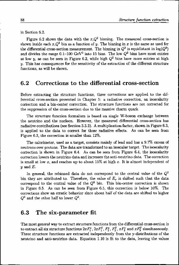
Figuree 6.2 shows the data with the x,Q2 binning. The measured cross-section is shownn inside each x,Q2 bin as a function of y. The binning in x is the same as used for thee differential cross-section measurement. The binning in Q2 is equidistant in log(Q2) andd divides the range 0.1-100 GeV2 into 15 bins. The low Q2 bins have most entries att low y, as can be seen in Figure 6.2, while high Q2 bins have more entries at high y.y. This has consequences for the sensitivity of the extraction of the different structure functions,, as wil l be shown.
6.22 Corrections to the differentia l cross-section
Beforee extracting the structure functions, three corrections are applied to the dif-ferentiall cross-section presented in Chapter 5: a radiative correction, an isoscalarity correctionn and a bin-center correction. The structure functions are not corrected for thee suppression of the cross-section due to the massive charm quark.
Thee structure function formalism is based on single W-boson exchange between thee neutrino and the nucleon. However, the measured differential cross-section has radiativee contributions (see Section 3.3.3). A multiplication factor, shown in Figure 6.3, iss applied to the data to correct for these radiative effects. As can be seen from Figuree 6.3, the correction is smaller than 12%.
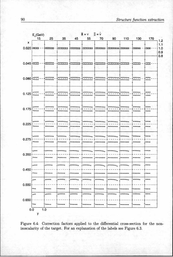
Thee calorimeter, used as a target, consists mainly of lead and has a 9.7% excess of neutronss over protons. The data are transformed to an isoscalar target. The isoscalarity correctionn is shown in Figure 6.4. As can be seen from Figure 6.4, the isoscalarity correctionn lowers the neutrino data and increases the anti-neutrino data. The correction iss small at low x, and reaches up to about 15% at high x. It is almost independent of yy and E.
Inn general, the rebinned data do not correspond to the central value of the Q2
binn they are attributed to. Therefore, the value of Ev is shifted such that the data correspondd to the central value of the Q2 bin. This bin-center correction is shown inn Figure 6.5. As can be seen from Figure 6.5, this correction is below 10%. The correctionss show an erratic behavior since about half of the data are shifted to higher QQ22 and the other half to lower Q2.
6.33 The six-parameter fit
Thee most general way to extract structure functions from the differential cross-section is too extract all six structure functions 2xF{, 2xFf, F%, F j , xF% and xF% simultaneously. Threee structure functions are extracted independently from the y-distributions of the neutrinoo and anti-neutrino data. Equation 1.10 is fit to the data, leaving the values
Figuree 6.3: Correction factors applied to the differential cross-section to correct for radiativee effects. Each plot represents the correction factor as a function of y. The correspondingg value of x is indicated on the left, the corresponding value of E on the top.. The scale is indicated on the right.
900 Structure function extraction
Ev(GeV)) Ï = v 5 = v 155 25 35 45 55 70 90 110 130 170
Figuree 6.4: Correction factors applied to the differential cross-section for the non-isoscalarityy of the target. For an explanation of the labels see Figure 6.3.
Figuree 6.5: Correction factors applied to the differential cross-section to shift the neu-trinoo energy such that the value of Q2 corresponds to the center of the bin. For an explanationn of the labels see Figure 6.3.
Figuree 6.6: Example of a six-parameter structure function fit to the differential cross-sectionn at x = 0.175 and Q2 = 8.2 GeV2. Errors are statistical only.
off all six structure functions free in the fit. The fit is obtained by minimizing the x2> usingg the MINUI T [39] package. An example of the six-parameter fit for one x,Q2
binn is shown in Figure 6.6. Note the strong correlation (p in Figure 6.6) between the measuredd values, in particular between 2xF\ and xF3.
Sincee the cross-section dependence on y is used to determine the different structure functions,, a sufficient range of y values is needed for a given x,Q2 bin. Therefore, only thosee x,Q2 bins are used for which the cross-section has been measured at four or more differentt values of y, of which at least one with y > 0.5. The systematic uncertainties havee been evaluated by repeating the fit eight times, applying the same systematic shifts appliedd before to the differential cross-section measurement, and adding in quadrature thee differences with respect to the central value.
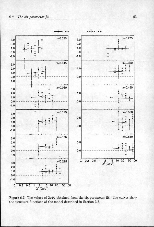
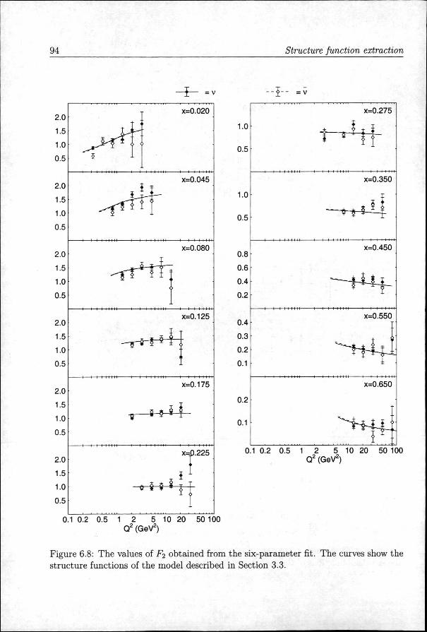
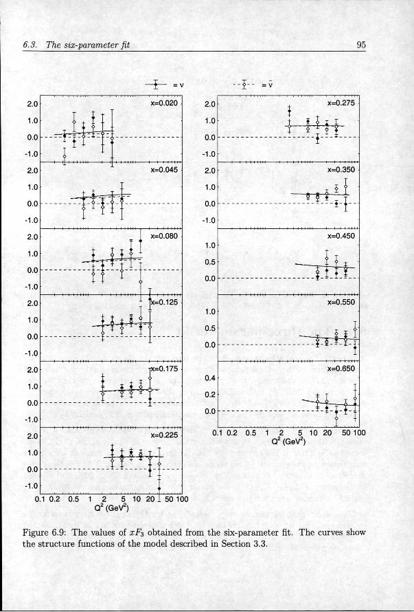
Thee results of the six-parameter fit are shown in Figures 6.7 to 6.9. It can be seenn that the statistical uncertainties of the structure functions extracted this way are large,, in particular for 2xF\ and xF3. No significant difference is observed between the neutrinoo and anti-neutrino structure functions.
6.3.6.3. The six-parameter fit 93 3
-l" -l"
0.11 0.2 0.5 1 Q22 (GeV2)
55 10 20 50 100
3.0 0 2.0 0 1.0 0 0.0 0
-1.0 0
1.0 0
0.0 0
1.0 0
0.0 0
0.5 5
0.0 0
0.5 5
0.0 0
x=0.275 5
—t—t—I—I I I I H I —i—>> i m i
II M I M I 1 1 l i t !
x=0.450 0
—i—ii i u r n 1 1—i-
ii •!• M I I 1 1 1—I I I I t I
x=0.650 0
0.11 0.2 0.5 1 2 5 10 20 50 100 Q22 (GeV2)
Figuree 6.7: The values of 2xFi obtained from the six-parameter fit. The curves show thee structure functions of the model described in Section 3.3.
944 Structure function extraction
x=0.020 0
-HH 1——( I I I I I II 1 1 1—
x=0.045 5
x=0.080 0
II I Ml 1 1 1 I H i l l 1 1 1 H I M
x=0.125 5
x=0.175 5
--
—I—II H-t-M 1 I—I—t—t-t
x=0.225 5
4-M--
0.11 0.2 0.5 1 2 5 10 20 50 100 Q22 (GeV2)
1.0} }
0.5 5
1.0 0
0.5 5
0.8 8
0.6 6
0.4 4
0.2 2
0.4 4
0.3 3
0.2 2
0.1 1
0.2 2
0.1 1
x=0.275 5
t-^ff f —II 1—I—t—<
x=0.350 0
x=0.450 0
—M4f--II I t II 1 1 1 I H i l l 1 1 1 I I I I
x=0.550 0
tt I—I I I I
x=0.650 0
" * f + l l 0.11 0.2 0.5 1 2 5 10 20 50 100
Q22 (GeV2)
Figuree 6.8: The values of F2 obtained from the six-parameter fit. The curves show the structuree functions of the model described in Section 3.3.
6.3.6.3. The six-parameter fit 95 5
„ v
0.11 0.2 0.5 1 55 10 20 Q22 (GeV2)
500 100
2.0 0
1.0 0
0.0 0
-1.0 0
2.0 0
1.0 0
0.0 0
-1.0 0
1.0 0
0.5 5
0.0 0
1.0 0
0.5 5
0.0 0
0.4 4
0.2 2
0.0 0
x=0.275 5
-\-\ 1 I I I I I I I
-HH H —H—II t t I t
x=0.350 0
ITgJ J
x=0.450 0
x=0.550 0
^éé ^éé tt t 1 I I I I I I t 1 ( I I I M I I I
x=0.650 0
0.11 0.2 0.5 1 2 5 10 20 50 100 Q22 (GeV2)
Figuree 6.9: The values of xF$ obtained from the six-parameter fit. The curves show thee structure functions of the model described in Section 3.3.
966 Structure function extraction
x=0.1755 Q2= 8.2 GeV2 J = v $ = v
"v,, 3.0 o o
CM M
E E o o CO O CO O
'oo 2.0
e e
SS 1-0
0.00 0.2 0.4 0.6 0.8 1.0 y y
Figuree 6.10: Example of the three-parameter structure function fit to the differential cross-sectionn for x = 0.175 and Q2 = 8.2 GeV2. Errors are statistical only.
6.44 The three-parameter fit
Inn general, the statistical precision of the structure functions can be improved by restrictingg the number of free parameters in the fit using for example the parton model relationss 2xF" = 2xF" and F2" = F2". The number of free parameters is then reduced too four, namely 2x.Fi, F2, xFz averaged for neutrinos and anti-neutrinos, and AXF3 = xF£xF£ — xFg. However, these two constraints alone do not improve significantly the statisticall precision, because of the high correlation between 2xFx and AxF3.
Iff either 2x.Fi or AxF3 is constrained, it is possible to extract the other with im-provedd statistical precision. In the kinematical domain of this analysis, AxF3 is ex-pectedd to be small. It can be relatively well constrained by the measured strange quark distributionn in the structure function model described in Section 3.3. For the three-parameterr fit presented in this section, a systematic uncertainty of 20% is attributed too the values of AxF3. The three-parameter fit results in a measurement of 2xFi, F2
andd XF3 averaged over neutrinos and anti-neutrinos.
Thee requirement on the range of y values for each x,Q2 bin is less strict than for the six-parameterr fit. Al l x,Q2 bins are used for which the cross-section has been measured att two or more different values of y, of which at least one has y > 0.4. The result of thee three parameter fit for a given x,Q2 bin is shown in Figure 6.10. The statistical
precisionn of the extracted values of the structure functions are typically an order of magnitudee better than those of the six-parameter fit, and the correlations between the threee structure function values are considerably smaller.
Systematicc uncertainties have been evaluated by repeating the measurement nine timess applying the same eight systematic shifts applied before to the differential cross-sectionn measurement and adding in quadrature the differences with respect to the centrall value. In addition, a la shift in AxF3 has been applied. The effect of each of thee systematic shifts on F2 and XF3 is similar as in the two-parameter fit and will be discussedd in Section 6.5. The effect on 2xF\ is covered by the systematic study on i?, andd will be discussed below.
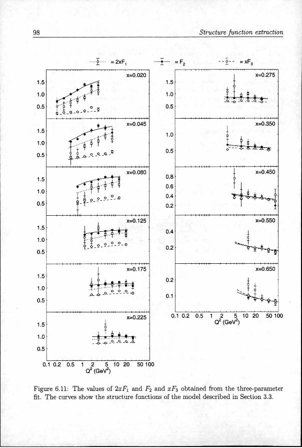
Thee results of the three-parameter fits are shown in Figure 6.11. All three structure functionss show a positive slope with respect to log(Q2) at low x and a negative slope att high x, in agreement with the scaling violations expected from QCD. At high x, the differencee between F2 and xF3 is small, while at low x, F2 is much larger than xF3. The differencee between F2 and xF3 can be interpreted as the sea quark distribution, which iss indeed concentrated at low x. The measurements show further that 2xF\ < F2 at loww x, indicating violation of the Callan-Gross relation.
Combiningg the measurements of 2x.Fi and F2, R is can be determined as follows:
Inn the determination of 5Ry the statistical uncertainty of R, the correlation between thee extracted values of 2xFi and F2, p(2xFi, F2), is taken into account:
/rmaa (, 2\2\(6{F2)\2 (F26{2xFl)\
2 F2 „„.-,„ „ '
(6.2) )
Thee systematic error on R has been evaluated in the same way as for the structure functionss (see above). The effect of the systematic shifts on R is shown in Figure 6.12. Ass can be seen from Figure 6.12, the dominant systematic effect is the uncertainty on thee hadronic energy scale.
Thee obtained values of R are shown in Figure 6.13, together with the parame-terizationn of the world data [19]. The data that correspond to Ehad < lOGeV are nott shown, because the precision of 2xFi is too poor. The measurements show that RR is significantly positive at low x (and low Q2), in agreement with the world data parameterization. .
—(( 1 t t 4 t*i 1 1 1—I I l l l l 1 1 1 - - * • • • • ! +•
x=0.350 0
x=0.550 0
—I—tt l l t »tt 1 1—I—I l l l l l
x=0.650 0
"̂4̂ ^ 0.11 0.2 0.5 1 2 5 10 20 50 100
Q22 (GeV2)
Figuree 6.11: The values of 2xF\ and F<i and xF$ obtained from the three-parameter fit .. The curves show the structure functions of the model described in Section 3.3.
6.5.6.5. The two-parameter fit 99 9
aa \>t +2.5% opp +150MeV
*o(v)+2.1% % TT o(v/v) +1.4%
o(v) +1 %/1 OOGeV o AXF3 +20% o(v/v)+0.5%/100GeV
x=0.020 0
—tt 1—i—i m i l 1 1—i i I I H I
x=0.045 5
x=0.125 5
—ii 1—i i m i l 1 1—I I I 11 M i 1—i i i i i
x=0.175 5
x=0.225 5
0.11 0.2 0.5 1 2 5 10 20 50 100 Q22 (GeV2)
0.2 2
0.0 0
0.2 2
0.0 0
0.2 2
0.0 0
0.2 2
0.0 0
0.2 2
0.0 0
x=0.275 5
-- ty '0 0—5 -
x=0.350 0
x=0.450 0
M i l ll 1 1—t—t-1 I t 11 1 1—I i-i
x=0.550 0
II I I I I I II 1— tt I 1 I t t I
x=0.650 0
0.11 0.2 0.5 1 2 5 10 20 50 100 Q22 (GeV2)
Figuree 6.12: Absolute effect on R of l a shifts of the nine systematic uncertainties.
1000 Structure function extraction
x=0.020 0
—H—i—ii n m
x=0.045 5
—ii I 1 4—1
x=0.080 0
- ii 1—i i i i i i i 1——i—i i i i i 11 1 1—i i m i
x=0.125 5
1 1 I M *
x=0.175 5
—II 1 1—t * i t-H 1 1—
x=0.225 5
0.11 0.2 0.5 1 2 5 10 20 50 100 Q22 (GeV2)
0.5 5
0.0 0
0.5 5
0.0 0
0.5 5
0.0 0
0.5 5
0.0 0
0.5 5
0.0 0
—i—II I 1 I I I
x=0.350 0
—II 1—I I M
x=0.450 0
1—i—ii i 11
x=0.55OJ J
x^.650, ,
0.11 0.2 0.5 1 2 5 10 20 50 100 Q22 (GeV2)
Figuree 6.13: The values of R = OLIO~T obtained from the three-parameter fit. The curvee shows the parameterization of the world data.
6.5.6.5. The two-parameter fit 101 1
x=0.1755 Q2= 8.2 GeV2 I-vf r r
LL 3.0
xF33 = 0.871 5
p(F2,xF3)) =0.089
X2=26.3/22(p=0.241) )
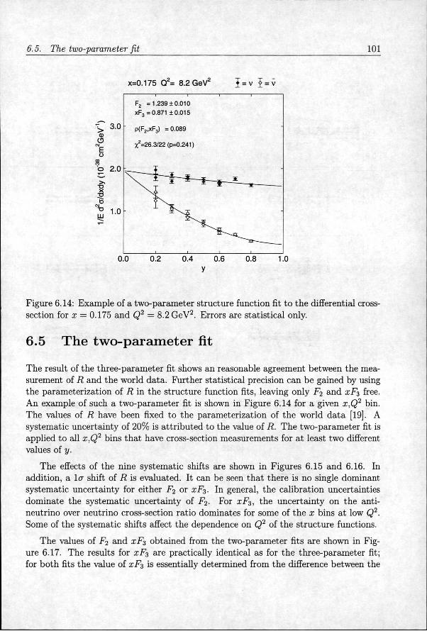
Figuree 6.14: Example of a two-parameter structure function fit to the differential cross-sectionn for x = 0.175 and Q2 = 8.2 GeV2. Errors are statistical only.
6.55 The two-parameter fit
Thee result of the three-parameter fit shows an reasonable agreement between the mea-surementt of R and the world data. Further statistical precision can be gained by using thee parameterization of R in the structure function fits, leaving only F2 and xF3 free. Ann example of such a two-parameter fit is shown in Figure 6.14 for a given x,Q2 bin. Thee values of R have been fixed to the parameterization of the world data [19]. A systematicc uncertainty of 20% is attributed to the value of R. The two-parameter fit is appliedd to all x,Q2 bins that have cross-section measurements for at least two different valuess of y.
Thee effects of the nine systematic shifts are shown in Figures 6.15 and 6.16. In addition,, a l a shift of R is evaluated. It can be seen that there is no single dominant systematicc uncertainty for either F2 or xF3. In general, the calibration uncertainties dominatee the systematic uncertainty of F2. For xF3, the uncertainty on the anti-neutrinoo over neutrino cross-section ratio dominates for some of the x bins at low Q2. Somee of the systematic shifts affect the dependence on Q2 of the structure functions.
Thee values of F2 and xF3 obtained from the two-parameter fits are shown in Fig-uree 6.17. The results for xF3 are practically identical as for the three-parameter fit; forr both fits the value of xF3 is essentially determined from the difference between the
Figuree 6.17: Values of F2 and xF3 obtained from the two-parameter fit. The curves showw the structure functions of the model described in Section 3.3.
6.6.6.6. Comparison with other neutrino experiments 105 5
neutrinoo and the anti-neutrino cross-section, and is almost independent of R. The sta-tisticall precision of i*2 has improved with respect to the three parameter fit, however, thee total uncertainty has not decreased significantly, because the systematic uncertainty dominates. .
6.66 Comparison wit h other neutrin o experiments
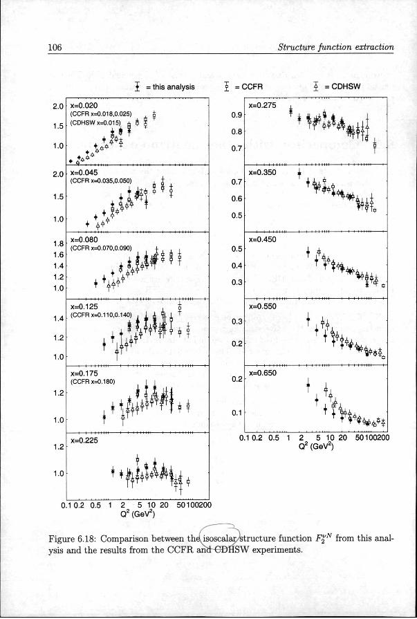
Thee results obtained in Section 6.5 for F2 and xF$ using the two-parameter fit are comparedd with those of two other experiments, namely CCFR [38] and CDHSW [37]. It shouldd be noted, however, that CCFR corrected for the charm production suppression, whereass no such correction was used by CDHSW or in this analysis.
Thee comparison of the structure function F2 is shown in Figure 6.18. The known discrepancyy between CCFR and CDHSW is clearly visible. The results from this analysiss agree better with CCFR in the region where the data overlap. The results of thiss analysis disagree with the CDHSW data, as observed before in the comparison of thee differential cross-sections (see Section 5.5). At low x, the data obtained from this analysiss are higher than CDHSW, while at high x they are lower. Due to the large systematicc uncertainties and the discrepancy between CCFR and CDHSW, it is not possiblee to determine an unambiguous nuclear dependence of F%N.
Thee CCFR data have been shown to be in good agreement with the charged lepton dataa [20], supporting the universality of parton distribution functions. However, at loww x, the CCFR data exceed the charged lepton data by 10-15%, which is beyond the quotedd statistical and systematic errors. The observed discrepancy has been confirmed inn a recent reanalysis, focusing on the low Q2, low x region [40]. Since the present measurementt agrees with the CCFR data, a similar disagreement will to show up in a comparisonn of this measurement with charged lepton data.
Thee comparison of the structure function xF$ is shown in Figure 6.19. The results fromfrom this analysis are in reasonable agreement with CCFR, but indicate a different x dependencee than CDHSW, similar as observed for F2.