UvA-DARE is a service provided by the library of the University of Amsterdam (http://dare.uva.nl) UvA-DARE (Digital Academic Repository) Wake Me Up Before You CoCo Chan, S. Link to publication Citation for published version (APA): Chan, S. (2017). Wake Me Up Before You CoCo: Implications of contingent convertible capital for financial regulation General rights It is not permitted to download or to forward/distribute the text or part of it without the consent of the author(s) and/or copyright holder(s), other than for strictly personal, individual use, unless the work is under an open content license (like Creative Commons). Disclaimer/Complaints regulations If you believe that digital publication of certain material infringes any of your rights or (privacy) interests, please let the Library know, stating your reasons. In case of a legitimate complaint, the Library will make the material inaccessible and/or remove it from the website. Please Ask the Library: http://uba.uva.nl/en/contact, or a letter to: Library of the University of Amsterdam, Secretariat, Singel 425, 1012 WP Amsterdam, The Netherlands. You will be contacted as soon as possible. Download date: 18 May 2018
Transcript
UvA-DARE is a service provided by the library of the University of Amsterdam (http://dare.uva.nl)
UvA-DARE (Digital Academic Repository)
Wake Me Up Before You CoCo
Chan, S.
Link to publication
Citation for published version (APA):Chan, S. (2017). Wake Me Up Before You CoCo: Implications of contingent convertible capital for financialregulation
General rightsIt is not permitted to download or to forward/distribute the text or part of it without the consent of the author(s) and/or copyright holder(s),other than for strictly personal, individual use, unless the work is under an open content license (like Creative Commons).
Disclaimer/Complaints regulationsIf you believe that digital publication of certain material infringes any of your rights or (privacy) interests, please let the Library know, statingyour reasons. In case of a legitimate complaint, the Library will make the material inaccessible and/or remove it from the website. Please Askthe Library: http://uba.uva.nl/en/contact, or a letter to: Library of the University of Amsterdam, Secretariat, Singel 425, 1012 WP Amsterdam,The Netherlands. You will be contacted as soon as possible.
Wake Me Up Before You CoCo:Implications of Contingent Convertible Capital for Financial Regulation
Contingent convertible capital (CoCo) is designed to improve the loss absorption capacity of the issuing bank without resorting to new equity or taxpayer-funded bailouts. However attractive they might seem to the regulator, they may have undesirable and unexpected consequences. This dissertation examines the implications of issuing CoCos for the financial system. For instance, CoCo conversion may be construed as signal about the asset quality of the bank, which may lead to contagious bank runs in the system. Another is that if the CoCo is inappropriately designed, the bank may accelerate the conversion by choosing high levels of risk to increase the bank’s residual equity value. Finally, the regulator’s desire for a trigger that she can control is an invitation for regulatory forbearance, which is what she was trying to avoid in the first place. Stephanie Chan (1984) holds a BSc in Economics and Accountancy from De La Salle University – Manila. She obtained a Master’s degree in Applied Economics from the same institution. In between, she was part of the Advisory group of PricewaterhouseCoopers Philippines. She obtained her MPhil from the Tinbergen Institute in 2013 and joined the UvA in the same year to write her PhD thesis on CoCos.
Wake Me Up Before You CoCo:
Implications of Contingent Convertible
Capital for Financial Regulation
ISBN 978 90 3610 483 8
Cover Design: Crasborn Graphic Designers bno, Valkenburg a.d. Geul
This book is no. 693 of the Tinbergen Institute Research Series, established through
cooperation between Rozenberg Publishers and the Tinbergen Institute. A list of books which
already appeared in the series can be found in the back.
Wake Me Up Before You CoCo:
Implications of Contingent Convertible Capital for Financial Regulation
ACADEMISCH PROEFSCHRIFT
ter verkrijging van de graad van doctor
aan de Universiteit van Amsterdam
op gezag van de Rector Magnificus
prof. dr. ir. K. I. J. Maex
ten overstaan van een door het College voor Promoties ingestelde
commissie, in het openbaar te verdedigen in de Aula der Universiteit
op vrijdag 9 jun 2017, te 11:00 uur
door
Stephanie Chan
geboren te Manilla, Filipijnen
Promotiecommissie:
Promotor: Prof. dr. S. J. G van Wijnbergen Universiteit van Amsterdam
Prof. dr. E. C. Perotti Universiteit van Amsterdam
Overige leden: Prof. dr. F. Allen Imperial College London
Prof. dr. A. W. A. Boot Universiteit van Amsterdam
Prof. dr. A. J. Menkveld Vrije Universiteit
Dr. W. E. Romp Universiteit van Amsterdam
Dr. T. Yorulmazer Universiteit van Amsterdam
Faculteit: Economie en Bedrijfskunde
Acknowledgements
My first day in Amsterdam was terrible: I took the train to the wrong direction at nighttime,
all the shops were closed, I was growing weak from hunger, I had no internet access, and my
mobile phone died! It foreshadowed the difficulties I would encounter while going through the
MPhil and the PhD stages: I took quite a lot of wrong turns and ran into a lot of dead ends
until I was finally able to find something that works. The process had not been easy, but one
eventually finds a way (or more). I knew nothing about the world upon arriving in Amsterdam,
but after six years in this lovely city, I can honestly say that I have grown up here. I want to
thank mentors, colleagues, friends and family, who helped in this venture.
I would first like to thank Sweder van Wijnbergen, for having faith in my small idea when
no one else did, and for taking me in for the PhD. He always challenged me to do my best,
and goaded me to believe in myself. I am very happy to have been his student, and I hope
that we can continue laughing and collaborating in the future. Enrico Perotti’s courses at the
Tinbergen Institute and the UvA defined my research interests. His remarks about my MPhil
thesis enabled me to reshape it into my first PhD essay. To the members of my dissertation
committee, thank you for taking time to read my work. I especially thank Franklin Allen and
Tanju Yorulmazer for their support during the job market period. I hope to make both of them
proud within the foreseeable future. Adriaan Soetevent, in his capacity as the Tinbergen DGS,
did not give up on me while I was floundering during the MPhil, and for that I am grateful.
The lovely ladies and gentlemen of MInt have been very supportive during the course
of the PhD: Franc Klaassen, Massimo Giuliodori, Kostas Mavromatis, Ward Romp, Christian
The creation of new banking regulation can hardly be described as a smooth process, because
there are many conflicting elements that a regulator must accomodate. For instance, the reg-
ulator must be careful to create rules that will not stifle the industry. At the same time, the
regulator must have sufficient political will to carry out its mandates, one of which is to pro-
tect the financial system from risks. The final form of any set of rules results from a protracted
period of consultation between the industry and the regulator.1 However, the final outcome
will only be as good as the foresight and intentions of the individuals involved. It is not incon-
ceivable that the industry would put forward suggestions that maximize their own benefit, but
impose negative externalities upon the financial system. As noted by Boyer and Ponce [2012]
and Hardy [2006], regulatory capture is a common occurence in banking supervision.
Also, even if regulation was well-intentioned to start with, it is not always the case that
all the possible consequences have been examined. I present two examples that by now have
become textbook fodder: securitization and risk-weighted assets. The intention of allowing
banks to securitize their loans was to allow them to dispose of nonperforming loans. However,
since the type of loans wherein securitization was allowed was not specified, banks were able
to game the system. The banks no longer cared about the quality of loans that they have been
extending, since they were able to eliminate those loans off their balance sheets. As for the
risk weights in Basel II, they were intended as a refinement of the crude risk weights in Basel I.
However, it retained the relatively low weight assigned to mortgages, reflecting the belief that
collateralized loans were safer than others. Without intending to, this led to an increase in the
demand for housing, leading to a bubble, and eventually contributed to the financial crisis of
1For the consultative documents pertaining to Basel III, the maximum number of days between the release ofthe consultative document and the deadline for comments is 127 days. The number of nonanonymous commentsranged from 6 to 121. Most of the comments came from banks and banking associations, with the occasionalacademic in the mix.
1
2007.
There are many possible reasons for the incomplete analysis of the impact of regulation
on the financial system. I present three of them here. One of them is the relatively short time
frame wherein the said rules were prepared. This is not surprising, considering that regulation
is usually formed as a reaction to adverse events.2 Around the period when Bear Stearns was
making headlines, regulators were already making changes to the system. Proposed revisions
to the market risk framework of Basel II had been set into motion in July 2008, and shortly after,
the first proposals to move towards Basel III were made. The Dodd-Frank Act was proposed
in July 2009 and finalized one year later. While new regulation has remedied the most obvious
problems, they have not fixed the underlying ones. Acharya [2011] has criticized both the
Dodd-Frank Act and Basel III for not being mindful of the impact of regulation on incentives
for the agents in the financial system.
The second reason for the incomplete analysis is that most of the new rules are add-ons
to existing regulation, in an effort to address problems that crop up. The problem with this
approach is that there is a tendency to create kludges3 in the financial system. This is not
to say that new regulation is completely harmful to the system. For instance, the increase in
capital requirements brought about by Basel III and Dodd Frank has made the financial system
relatively safer in the sense that the financial system is more able to withstand shocks.
Finally, financial innovations are being created at the same time as new rules are, leading to
unexpected interactions. For instance, Blundell-Wignall and Atkinson [2010] note that credit
default swaps arose at the same time that the refined risk weighted asset bucket weights did,
which allowed the banks to undermine the fundamental idea of capital weights. It is because of
such unexpected events that regulatory discretion is important. In particular, Pillar 2 of Basel
II is meant to deal with bank-specific uncertainties. However, there must be a balance between
rules and discretion. This does not seem to be the case, if one contrasts the voluminous require-
ments of Basel II’s Pillar 1, against the free rein that supervisors have in Basel II’s Pillar 2. This
is important because there is a tendency for regulators to forbear on tough decisions, because
of short term gains that may be foregone. Numerous papers have been written on regulatory
forbearance (see Mailath and Mester [1994] and Shapiro and Skeie [2015] for instance). The
problem with forbearing on tough decisions is that the system may survive in the short term,
but may be more fragile in the long term.
With all these issues, it is not surprising that regulators are always on the lookout for
2The time it takes to get from the proposal to the final document stage has high variance: for Basel II, it took6 years, for Basel III and the Dodd-Frank Act, it took around one year each.
3The Merriam Webster Dictionary defines kludge as "a system and especially a computer system made up ofpoorly matched components."
2
new tools that appear to address the problems they have encountered. For instance, shortly
after the financial crisis of 1933 when bank failures were contagious, deposit insurance became
prevalent (Federal Deposit Insurance Corporation [1998]). However, as is now widely known,
deposit insurance alters the banking system’s incentives and encourages moral hazard. Most
recently, regulators have encouraged the adoption of contingent convertible capital (CoCo),
in light of the high cost of bailing out financial institutions during the financial crisis of 2007.
CoCos are hybrid instruments that are issued by banks as debt, but convert to equity or are
written down upon the occurence of a trigger event.4 Upon the occurence of a conversion, the
issuer’s loss absorption capacity increases, without the involvement of the government or the
taxpayers. Instead, the holder of the CoCo shoulders the losses. For this reason, CoCos have
become very attractive to regulators,5 and their use has been passed into law in Europe. But if
history is a guide, regulators should realize that there is always more to financial innovation
than meets the eye. It is crucial that the properties of CoCos be deeply investigated before
rolling it out on a wide basis. This dissertation is a step in that direction.
1.1 A short primer on CoCos
CoCos are hybrid instruments that are designed to improve the loss absorption capacity of the
issuer without involving transfusions from new equity or taxpayer bailouts. These instruments
were proposed by Flannery as early as 2002, but were thrust into the limelight after the financial
crisis of 2007. Banks generally issue CoCos, though the insurance sector has already started
looking into them aswell. CoCos are issued as debt, butwhat happens after conversion depends
on the type of CoCo issued. There are generally two types of CoCos based on design: principal
writedown (PWD) CoCos are partially or fully written off the balance sheet, while convert-to-
equity (CE) CoCos are converted to shares at a preset price.
There are two type of trigger events: automatic and discretionary. Automatic trigger events
occur when the bank’s equity ratio falls below a preset amount. The calculation may be based
on either market or book values, although all of the issued CoCos so far have calculations
based on book value. Discretionary trigger events occur when the regulator deems the bank
to be near or at the point of nonviability (PONV). Because of the nature of the trigger event,
CoCos have also been known as reverse convertible bonds, because they convert when there is
a negative event, rather than a positive one (as ordinary convertibles do). To qualify as part of
4The trigger event is when the issuer’s equity ratio falls below a preset threshold, or when the regulatorassesses that the bank is close to the point of nonviability.
5More recently, the Financial Stability Board has created demand for CoCos by requiring globally systemicbanks to increase their loss absorption capacity by CoCo issuance.
3
regulatory capital under Basel III, CoCos must have at least the discretionary trigger. Because
of this, most of the issued CoCos possess both types of triggers.
Figure 1.1 presents the European issuances of CoCos by design.
Figure 1.1: Annual CoCo Issuance of European Banks by Design
2.8
.4 0
2.8
8
0
8.4
3.4
1.5
16.3
7.2
0
25.8
20.4
0
19.7
14.5
0
12.9
10.6
0
05
1015
2025
in b
illio
n E
uros
2010 2011 2012 2013 2014 2015 2016
Annual CoCo Issuance of European Banks by Design
PWD CEN/A
Source: Dealogic (through the Association for Financial Markets in Europe)
It is notable that PWD CoCo issuances have overtaken CE CoCo issuances since 2012. By
the end of 2016, PWD CoCos amounted to 57% of total European issuances, while 43% were
CE CoCos, and less than 1% were of an unspecified type. Most of the CoCo issuance is by
European and Asian banks. US banks have not participated in the wave of CoCo issuances
because CoCos are treated as equity under US GAAP and as such, do not have tax benefits.
Because of their loss absorption capacity, CoCos have made their way into formal regula-
tion. In June 2011, the Basel Committee on Banking Supervision released the final version of
Basel III, which addresses additional measures to ensure the stability of the banking system.
One notable change from Basel II is the strengthening of the capital base by enforcing stronger
requirements for regulatory capital: loss absorption capacity is now a necessary quality for
instruments to be included as part of Additional Tier 1 (going concern) capital and Tier 2 (gone
concern) capital. Existing instruments that no longer qualify as regulatory capital have been
phased out beginning January 2013, and replaced by CoCos. The criteria for whether a CoCo
falls under Additional Tier 1 or Tier 2 depends only on their trigger level: above 5.125% quali-
fies as Additional Tier 1, otherwise they qualify as Tier 2. Figure 1.2 shows the distribution of
the European-issued CoCos by their trigger ratios.
4
Figure 1.2: European CoCo Issuances by Trigger Ratios
86
14
72
28
56
44
020
4060
8010
0in
per
cent
2014 2015 2016
Annual European CoCo Issuances by Trigger Ratios
AT1 T2
Source: Dealogic (through the Association for Financial Markets in Europe)
While Basel III itself has no legal bite, it was translated into EU law in 2013 by the issuance
of Directive 2013/36/EU, also known as the Capital Requirements Regulation and Directive
(CRR/CRD-IV). This means that for EU banks, at most 3.5% of the 8% regulatory capital re-
quirement will be filled in by CoCos. Moreover, there is no upper bound to the amount of
CoCos they can issue. In addition, in November 2015, the Financial Stability Board (FSB) has
released its Total Loss Absorption Capacity (TLAC) Standard for globally systemic financial in-
stitutions. The TLAC Standard mandates that for these institutions, minimum loss absorption
capacity must be raised to 16% of risk weighted assets by January 2019, and to 18% by January
2022. The TLAC Standard’s description of the loss absorbing instruments fits CoCos. With
this, one should see an increase in the CoCo issuances over the next few years.
As CoCos are new and not well-understood, steps have been taken to protect unwitting
consumers. In October 2014, the U.K.’s Financial Conduct Authority has prohibited banks from
issuing CoCos to ordinary retail investors. Moreover, the market has been shown to be sensi-
tive to potential trigger events. In February 2016, the price of CoCos issued by Deutsche Bank
fell from fears that the bank would not be able to meet its coupon payment obligations. How-
ever, the prices of other CoCos followed suit, despite the absence of adverse news regarding
their issuers.
5
1.2 Thesis outline
Upon first glance, CoCos appear to be exactly the type of instrument that regulators wish
for. Moroever, there are relatively few restrictions regarding the issuance of CoCos. One may
argue that CoCo conversion is a straightforward task. However, one must look at how these
rules will interact with the agents in the economy, as there may be undesirable and unexpected
consequences. For instance, the conversion of the CoCo may be construed as signal about the
asset quality of the bank, which may lead to contagious bank runs in the system, even for non-
CoCo issuers. Another is that if the CoCo is of the principal writedown type, the bank may
accelerate the conversion by choosing a high risk level, as doing so effectively increases the
bank’s residual equity value. Finally, the regulator’s desire for a trigger that she can control
is an invitation for regulatory forbearance, which is what she was trying to avoid in the first
place.
Throughout this dissertation, we take the capital structure as a given. This is because banks
are not able to instantaneously adjust their capital structures as the situation changes. Also,
throughout this dissertation, we take the CoCo holders as passive agents. If CoCos are correctly
priced, the CoCo holders are sufficiently compensated for the risk they bear, and therefore lose
any incentive to monitor the bank. But also it is only once the CoCo is issued that all the
other agents act. Banks may decide to risk-shift, depositors may run, and the regulator may
decide never to convert CoCos at all. These events are not very obvious consequences of CoCo
issuance. In each chapter, we consider different settings under which CoCos are issued, and
examine how different agents behave under the settings, as well as the consequences. We
do this with a variety of methods, but use three period models to make them as tractable as
possible.
In Chapter 2, "CoCos, Contagion, and Systemic Risk," jointly written with Sweder van Wi-
jnbergen, we examine the CoCos that convert upon regulatory discretion. We abstract away
from bank decision-making, focusing instead on how the regulator’s decision to convert af-
fects the depositors’ running decisions. We assume that the regulator has better information
about the economic fundamentals compared to the rest of the agents in the economy. The reg-
ulator forces the conversion of CoCos when she obtains information that the bank is unlikely
to remain viable given the economic state. Therefore, conversion is always interpreted as a
negative signal, and results in a bank run. We apply global games in the spirit of Goldstein
and Pauzner [2005] in order to obtain a measure of the probability of bank runs, as well as to
eliminate the multiple equilibria issue that often arises in bank run models. The probability of
bank runs also determines the measure of agents that run. The number of agents that run, in
addition to the type of CoCo that is issued, have different impacts on a bank’s residual equity,
6
conditional on the bank surviving. Therefore, some CoCos are better than others ex post when
converted. The tension that the regulator faces between facing a bank run and increasing the
bank’s loss absorption capacity is highlighted, although in this chapter we do not take a stand
on it. Instead, we focus on the impact of a conversion on the financial system. Assuming that
asset returns are correlated, and increase in correlatedness during times of crisis, it becomes
clear that the bank runs become contagious whenever CoCos are converted. For this reason,
we argue that systemic risk increases upon CoCo conversion, which is surprising given that
they were intended to act as shock absorbers in the first place.
In Chapter 3, "CoCos, Risk-Shifting, and Financial Fragility," jointly written with Sweder
van Wijnbergen, we consider CoCos that convert automatically, without the intervention of
the regulator. We abstract away from the depositors by assuming deposit insurance, and this
allows us to assess whether banks would risk-shift more or less with CoCos in their capital
structure. We argue that because banks are able to choose their own risk levels, and that the risk
choice affects the return distribution, the probability that the CoCos convert is not exogenous.
Depending on the design of the CoCo, the bank potentially gains a wealth transfer from the
conversion. We argue that this motivates higher risk-shifting relative to standard instruments
like debt and equity. In order to show this, we use the language of call options. Since CoCos
contain elements of debt and equity, the valuation of the issuer’s residual equity must take
these elements into account. In particular, the issuer’s residual equity can be expressed as
residual equity with subordinated debt, plus an expected wealth transfer. However, we show
that for certain CoCo designs, the expected wealth transfer is increasing in the risk level chosen
by the bank. Therefore, whenever banks maximize their expected returns net of default costs,
they would always choose higher risk levels under these types of CoCos than under the same
amount of subordinated debt, or additional equity. The policy implication is that one cannot
treat CoCos as true substitutes for equity, because while they have the same loss-absorption
capacity, they induce different incentives. Finally, the use of CoCos as equity supplements
distorts the true level of equity required, relative to the same amount of subordinated debt
would, for the regulator to obtain a target probability of default that depends on the bank’s
leverage and risk levels.
In Chapter 4, "Regulatory Forbearance in the Presence of Cocos," jointlywrittenwith Sweder
van Wijnbergen, we again consider CoCos that convert upon regulatory discretion, and we
model the bank’s asset choices as well. We do this in order to focus on the interaction between
a regulator and a CoCo-issuing bank. In order to do this, we use a simple game-theoretic
three-period model. We give the bank two opportunities to commit moral hazard upon ob-
taining its funds: the initial asset choice at t = 0, and whether to gamble for resurrection or
7
to liquidate bad loans when they occur, at t = 1. In this setting, the bank will only choose
the socially optimal action (liquidate) if its skin in the game is high enough at t = 1. This is
where CoCoswould prove to be useful, as conversion reduces the bank’s outstanding liabilities.
However, if the regulator faces sufficiently high costs of conversion, she will always forbear
even if conversion improves a bank’s loss absorption capacity. We endogenize the regulator’s
cost of conversion by embedding depositors’ beliefs regarding asset quality into it. Essentially,
the cost of conversion is the marginal probability of a bank run based on depositors’ beliefs.
The regulator’s action as anticipated by the bank then feeds back into its t = 0 decision: if the
regulator is forbearing, the bank would choose the risky asset over the safe one as it provides
a larger private benefit for the bank. If the regulator was tough, conversion would only be a
sufficient risk deterrent at t = 1 if there were not too many CoCos issued to begin with. How-
ever, this again brings into the forefront the tradeoff between loss absorption capacity and risk
shifting of banks.
8
Chapter 2
CoCos, Contagion, and Systemic Risk1
2.1 Introduction and literature review
As early as 2002, Flannery proposed an early form of contingent convertible (CoCo) capital
that he called reverse convertible debentures.2 The idea was simple: whenever the bank issu-
ing such debentures reaches a market-based capital ratio which is below a pre-specified level
(say, 8% of assets), a sufficient number of said debentures would automatically convert to eq-
uity at the prevailing market price of the bank’s shares. The automatic conversion feature frees
the issuing bank from having to raise additional capital immediately when its capital ratio is
lower than the minimum requirement. For larger shocks, conversion may not be enough to re-
store compliance with capital requirements, but it would make banks merely undercapitalized
instead of bankrupt.
Flannery’s initial CoCo design proposal was attractive, as its automatic conversion feature
had the potential to avoid socially costly bailouts. After the 2007 financial crisis, regulators re-
alized that even though systemically important financial institutions (SIFIs) held Tier 2 Capital,
that type of capital failed to be loss-absorbing during the time of distress. Instead, some of the
SIFIs were bailed out while others were allowed to fail. Yet despite having Tier 2 status, many
of the subordinated loans continued to be serviced. In response, the Basel Committee on Bank-
1This chapter is based on Chan and van Wijnbergen [2014], which won the Best Conference Paper award atthe June 2016 IFABS meeting in Barcelona. We thank Franklin Allen, Olivier Blanchard, Arnoud Boot, CharlesCalomiris, Ieva Sakalauskaite, seminar paticipants at the IMF, Tilburg University, the Tinbergen Institute Amster-dam and participants at the DNB conference onmacroprudential regulation, in particular our discussant BenjaminKay for helpful comments and discussions. We also thank participants who gave comments at the the 2016 EEAmeetings.
2Unlike ordinary convertible bonds, reverse convertible debentures expose the holder to the potential down-side of holding equity
9
ing Supervision (BCBS) circulated a consultative document3 that was one of the precursors to
what is now known as Basel III. Among the changes were the redefinition of "gone concern"
to include potential bailout situations, and the inclusion of CoCo-like instruments as part of
Additional Tier 1 Capital.4 Also, Basel III suggested that CoCos might play a role in ensuring
that SIFIs would have higher loss absorption capacities than regular financial institutions.
The inclusion of CoCos as part of Additional Tier 1 Capital is a likely factor in the increase
of CoCo issuance. European CoCo issuances totaled 23.5 billion Euros in 2016, up from only
3.2 billion Euros in 2010.5 Within the same period, the academic literature branched off in
three different directions. Flannery [2005] and McDonald [2013] were among those that dealt
with design features such as triggers and bases. Pennacchi [2010] dealt with the pricing and
valuation of CoCos. Finally, Martynova and Perotti [2016], Hilscher and Raviv [2014] and Berg
and Kaserer [2015] consider the effect of CoCos on risk-taking incentives of banks. Moreover,
several survey articles have been written about CoCos. Maes and Schoutens [2012] provide
an overview of CoCos and enumerate the potential downside of CoCo issuance such as con-
tagion from the banking to the insurance sector, and the creation of a "death spiral" where
CoCo holders short-sell the stock of the issuing bank in order to profit from potential con-
version. Avdjiev et al. [2013] discuss the features of the CoCo trend - from the reason why
banks issue them to the main groups of investors that are interested in buying CoCos, as well
as the pricing of CoCos. Wilkens and Bethke [2014] summarize and empirically assess some
of the pricing models’ performance. There is disagreement in the literature on whether CoCo
conversion should be triggered based on market prices or book values (e.g. capital ratios used
under Basel III). On one side are authors like Sundaresan and Wang [2015], who argue that us-
ing market prices in calculating trigger values might lead to multiple equilibria problems and
potentially destabilizing bear runs on bank stock. On the other side, Calomiris and Herring
[2013] argue that this problem can be mitigated by using 90-day moving averages of what they
call "quasi-market data",6 arguing that using book values creates room for creative accounting
- for example pressure to delay recognition of losses. We do not take a position in this debate,
our analysis applies to both types of triggers.
The effectiveness of CoCos hinges on bank failure being caused by banks having insuffi-
cient equity to absorb losses once they have occurred. However, the majority of bank assets
is funded by demand deposits. One cannot ignore the possibility that a bank may fail because
3“Proposal to ensure the loss absorbency of regulatory capital at the point of non-viability”, Basel Committeeon Banking Supervision [2010]
4To be counted as Additional Tier 1, the instruments must meet several requirements set forth in Basel III.5Association for Financial Markets in Europe [2016d]6Calomiris and Herring [2013] define quasi-market data as a ratio of market value of equity and book value
of debt
10
depositors run before losses actually occur, as they anticipate what may happen once the losses
do occur. Jacklin and Bhattacharya [1988] and Chari and Jagannathan [1988] build on the Di-
amond and Dybvig [1983] model of bank runs to show that depositors who are able to update
their information about the realization of bank returns act accordingly. However, early bank
run models have the disadvantage that runs are zero probability events, sunspot equilibria.
That makes it impossible to assess the impact of fundamentals on the probability of runs and
the associated bank collapse. Goldstein and Pauzner [2005] take the Diamond-Dybvig model
a substantial step further by casting the standard banking problem into a global games frame-
work, allowing them to obtain a measure for the probability of a bank run which can be linked
to economic fundamentals.
In this paper, we argue that a CoCo conversion conveys information that will lead deposi-
tors to update their beliefs in amanner that increases the probability of bank runs. Furthermore
we examine three major types of CoCos7 and show that some designs are better than others in
terms of their effect on depositor run incentives. We make a second point that is crucial for the
relation between CoCo conversions and systemic risk. If other banks hold assets with corre-
lated returns, depositors of other banks will interpret the CoCo conversion as a negative signal
on their asset returns too. This updates the beliefs of the depositors of the other banks, which
raises the probability of runs on said banks, even if they were non-CoCo-issuing. This would
not happen if conversion did not occur in the CoCo-issuing bank. In other words, through
contagion effects conversion imposes an information externality on other banks, which raises
systemic risk.
The large and growing literature on contagion has by and large highlighted three contagion
types: Balance sheet contagion (through firesale effects, cf Diamond and Rajan [2011]), fund-
ing squeezes whereby distress in one bank causes liquidity to dry up for another bank (Luck
and Schempp [2014]), and information contagion (Ahnert and Georg [2016]). The contagion
channel that plays a role in our analysis falls in the third category: A CoCo conversion gives
out a signal about asset quality that triggers a run not only in the bank concerned but also in
banks with correlated assets.
This contagion channel is a second reasonwhywe expect CoCos to raise rather than reduce
systemic risk. This is worrisome also because CoCos are mentioned by Basel III as potentially
useful for increasing the loss absorption capacity of SIFIs. While it is true that conversion may
keep the issuing banks afloat in times of distress by immediately reducing their outstanding
liability, it does not reduce the liability to depositors. As such, conversion increases the risk
7At the time of writing, there were three types of CoCos issued: principal writedown CoCos, convert-to-equityCoCos, and principal writedown CoCos that pay out cash to the CoCo holders upon conversion. Currently, onlythe first two types remain.
11
that the converting banks, and other banks to the extent that they have correlated assets, will
face a run.8
While CoCos have different trigger points and conversion mechanisms, many of them have
a "point of nonviability" clause which effectively gives regulators control over when CoCos
convert. But regulators may end up having to make difficult choices in such circumstances. If
conversion actually raises systemic risk, microprudential and macroprudential considerations
may well be at odds, possibly leading to high pressure for regulatory forbearance.
2.2 Basic model
Bank runs arise due to asymmetric information regarding the need of depositors. Diamond
and Dybvig [1983] show that when bank returns are certain, banks can write contracts that
mimic the first best outcome that an omniscient social planner can implement, by taking the
type of depositor into account. However, because the type of each depositor is unknown to
the bank, a sequential service constraint is put in place. As there is nothing in their model that
coordinates the beliefs of depositors, two equilibria emerge: either a bank run occurs, or it does
not. Goldstein and Pauzner [2005] introduce the more realistic case of uncertain returns into
the Diamond and Dybvig [1983] model, where the probability of obtaining positive returns
depends on the economic fundamentals. In addition, they allow the depositors to have varying
beliefs about the true state of the economy, as opposed to sharing a singular belief. In this way,
the depositors are able to coordinate on something, thus eliminating the the multiple equilibria
problem in Diamond and Dybvig [1983], as well as obtaining a measure of the probability of
bank runs.
We extendGoldstein and Pauzner [2005] by addingCoCos and equity to the usual depositor-
only setup. This is becausewewant to highlight the tension between theCoCos’ loss-absorption
benefits and their potential impact on the probability of bank runs. This is impossible in stan-
dard bank run models, as they have no equity to speak of. Moreover, we add a zero-probability
event where the positive return is lower than expected. This is because we want to model
the situation where the regulator comes across more information than the rest of the agents,
and has decided to act upon it. Goldstein and Pauzner [2005] show that the probability of a
8It is sometimes argued that the threat of dilution from CoCo conversion encourages existing equity holdersto infuse at least enough additional capital to stave off conversion, rendering the signalling effect of conversionnonexistent. However, whether this incentive exists this depends on the CoCo design. In Chan and van Wijnber-gen [2017a] we show in that in several currently popular CoCo designs, wealth transfers upon conversion actuallygo from junior creditors to equity holders. This reduces the incentives for equity holders to supply capital in timesof distress, and may even reverse it. While by design equity holders cannot pull out capital, the existence of suchsuch a peverse incentive might induce them to push for additional risk taking by bank management.
12
run is increasing in the amount promised to the depositors who are impatient consumers. By
the same token, any factor affecting the relative return of the patient consumers will alter the
probability of a run. In a model where the lower returns will induce the regulator to convert
the CoCos, conversion definitely signals bad news and informs the agents that the return that
are worse than expected have materialized. This then leads to an increase in the probability of
a bank run.
2.2.1 Setup
Our model has three periods (t = 0, 1, 2), a bank, a regulator, and three types of agents, each
endowedwith one unit of wealth: n depositors, e−n CoCo holders, and 1−e equity holders. Thenotationwas chosen such that the total measure of agents is 1. We assume that themeasures are
fixed, as we are not interested in optimal capital structure. Figure 2.1 illustrates the continuum
of agents in this model.
Figure 2.1: Agent Types and Measures
0 n e 1
1− eequityholders
e− ncoco
holders
n depositors
At t = 0, the depositors, CoCo holders and equity holders essentially set up the bank
by investing their funds into it. In order to induce the agents to invest their funds, they are
promised returns: CoCo holders are promised some return rc , while depositors that withdraw
at t = 1 are promised some return r1 > 1. Equity holders obtain any residual profit. We assume
that in this model that the CoCo holders and the equity holders are risk-neutral and are long-
term investors (or alternatively, have long-term liquidity needs). In contrast, the n depositors
are risk averse with −cu′′(c )/u′(c ) > 1 for some c > 0. In addition, the depositors are uncertain
of their own liquidity needs at t = 0: a fraction λ will turn out to be impatient consumers who
can only consume at t = 1 with corresponding utility u (c1). The remaining 1 − λ will turn out
to be patient consumers who may consume at either t = 1 or t = 2, with corresponding utility
u (c1 + c2). At t = 0, there is no aggregate uncertainty: the proportion of impatient and patient
consumers is known. At t = 1, each depositor discovers his own type, and this remains private
information. Because the type of each depositor is unknown to the bank, a sequential service
constraint is put in place.
13
There exists an investment technology that the bank has access to. It delivers returns which
vary with the economic state θ ∼ U [0, 1]. A higher realization of θ indicates better economic
conditions. Specifically, one unit of investment at t = 0 yields R with probability p (θ ), and 0
with probability 1 − p (θ ) at t = 2. Also, we assume that p (θ ) is increasing in θ . Of course,
p (θ ) ∈ [0, 1]. The investment may be liquidated at t = 1 without cost other than the foregone
yield. At t = 1, there may be a shock to the economy that affects not the fundamental value θ ,
but the returnR. In particular, the returnmay be someRL < R, but is assigned a zero probability
at t = 0. This is because the shock is presumed to be unknown at t = 0, materializing only
at t = 1. In addition, each depositor has a belief θi about the economic fundamental θ that
is drawn uniformly from [θ − ε, θ + ε]. Depositors know the probability function p (·), butevaluate it at their own θi .
Because the risky investment can be liquidated without cost, agents are better off investing
their endowment into the asset. Also, we assume that R is high enough so that Eθp (θ )u (R) >
u (1), making it worthwhile for patient consumers to wait until t = 2. Without any pooling of
risk, the best attainable utility levels are u (1) for the early consumers and p (θ )u (R) for the late
consumers (for a given state of nature θ ).
Even with long term funding without early withdrawal possibilities, runs are still possible
as long as 1r1< n. We assume this throughout the paper. We furthermore assume that the
contracts offered by the banks are such that the incentive compatibility constraint u (r1) <
p (θ )u(1−λr11−λ R
)in fact holds: late consumers prefer towait. Finally, there is no deposit insurance
in this model.9
2.2.2 The regulator
Even though we have introduced CoCos in the model, we abstract away from the utility of the
CoCo holders. The value of CoCos in this model is in the signal that their conversion transmits
to the rest of the agents, as well as by increasing the bank’s equity levels upon conversion.
There are two ways that CoCos may be converted in practice: by accounting/market value
triggers, or by regulatory discretion. In ths paper we model the latter.
There is a regulator who is interested in preserving financial stability. In accordance with
the structure of many of the issued CoCos, we assume conversion occurs when the regulator
decides to trigger the conversion. We assume that the regulator when she decides to force
conversion knows more than the other agents: that a regulator may discover at t = 1 that
9Alternatively, theremay be deposit insurance for retail deposits but there are also large and substantial whole-sale deposits which are not insured. Or one can think of other forms of short term funding with roll over riskexposure like REPOs or commercial paper.
14
asset returns at t = 2 will be lower than what is compatible with a capital ratio above the
CoCos trigger value. In particular, we assume that the regulator finds out that the returns in
the good state of nature will be RL < R. Based on the finding, the regulator decides whether or
not to convert the CoCos. The regulator’s decision to intervene (or for that matter collect the
additional information about asset quality to begin with) is not modeled in this paper.10 But
as will be shown later, her decision to convert CoCos introduces a negative signal about asset
returns even though the economic fundamentals θ remain the same. We assume in this paper
that this regulatory inspection and its outcome are not anticipated (not priced in) by investors,
in particular by the deposit holders. In the wording of Gennaioli et al. [2013], the regulatory
intervention is a neglected risk. Zhou and van Oordt [2016] in fact show that tail risk events
are not priced in the case of similar securities (options).
2.2.3 Timing
First, let us consider the situation prior to conversion. By assumption, at t = 0, a fraction e − nof agents has invested in CoCos and a fraction 1 − e has invested in equity. The remaining n
are depositors whose types are unknown at t = 0.
With these agents’ endowments, the bank has a total of 1 unit of wealth. The bank invests
the entire amount in the risky asset. It also promises a fixed return r1 > 1 to depositors who
withdraw at t = 1, and a stochastic return that in the absence of runs by late consumers equals
r2 = max[n−λnr1n−λn R, 0
], depending on the state of nature that materializes at t = 2.11 Note that
this is similar to the Diamond and Dybvig [1983] contract since n−λnr1n−λn R = 1−λr1
1−λ R . Henceforth
we use rD for 1−λr11−λ R. Define n as the proportion of agents who withdraw at t = 1. Since early
consumers always withdraw at t = 1 , n ≥ λn. And because the CoCo holders and equity
holders cannot withdraw early, we also have n ≤ n.
At t = 1, before agents can act, the regulator comes in and decides whether to convert
CoCos or not. If conversion occurs, the return in the good state must have been found to be
some RL < R. In such a case, depositors’ return will be scaled downwards accordingly (they
will receive 1−λr11−λ RL instead of 1−λr1
1−λ R). Effectively, the depositors have a variable-rate contract
with the bank. Without conversion, no information is revealed. This still preserves the risk-
sharing feature of Diamond-Dybvig, which concerns not so much the interest rate risk as the
type-related liquidity risk.
Also at t = 1,depositor types are revealed. The bank gives r1 > 1 to depositors withdrawing
10One way to think of our set up is in line with the costly audit literature where audits, or in our case morelikely an on-site regulatory inspection, are performed only infrequently and possibly randomly
11Appendix 3.A.1 contains the calculations for this section.
15
at this time as long as it is able to do so. To this end, the bank must liquidate part of the amount
invested in the risky asset. This means that the bank can only serve at most n = 1r1agents at
t = 1. The t = 2 payoffs to the depositors in the no-conversion case are summarized in Table
2.1.
Table 2.1: Time-dependent payoffs to each depositor
Withdrawal in if λn < n < λn + e ′r1
if λn + e ′r1< n < 1
r1if n ≥ 1
r1
t = 1 r1 r1⎧⎪⎨⎪⎩r1 w.p. 1
nr1
0 w.p. 1 − 1nr1
t = 2 rD =1−λr11−λ R
⎧⎪⎪⎨⎪⎪⎩1−nr1
1−(λn+ e ′r1)r1rD w.p. p (θ )
0 w.p. 1 − p (θ )0
Depositors who wait until t = 2 to withdraw will receive a return which depends on how
many depositors ran at t = 1. CoCo holders and equity holders, being junior to depositors, will
receive amounts only once all the depositors have been served. How that surplus is divided
between them depends on CoCo pricing and corresponding CoCo returns. With probability
1 − p (θ ), the return (to creditors and equity holders alike) will be zero.
The bank can ensure that it pays out rD to the late consumers as long as λn < n < λn +e ′r1. This is because unlike Goldstein and Pauzner [2005], our model has additional sources of
funding from CoCo holders (e − n) and equity holders (1− e). Because depositors are senior toall other agents, these proceeds (call them e′ = (e − n) + (1 − e ) = 1 − n) may be exhausted in
order to pay out e ′r1more depositors at t = 1, and still manage to pay out rD to the remaining
depositors at t = 2.12
But for values of n between λn + er1and 1
r1, withdrawers at t = 2 may not obtain the entire
rD . As the bank’s resources are finite at 1 unit, there can be only at most n = 1r1depositors who
may be served at t = 1. In this case, the asset is fully liquidated - nothing is left to earn R in case
the good state of nature materializes at t = 2. Between n = λn + er1and n = 1
r1, each additional
runner requires further liquidation of the long-term asset, leaving a smaller quantity of the
asset to potentially earn R. One can then determine the rate at which rD erodes - it depends
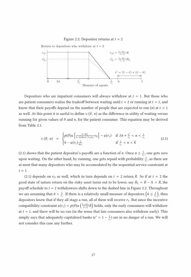
on n. Figure 2.2 shows the payoffs to depositors who wait until t = 2 as a function of n under
different levels of asset returns.12Note that the region where money paid out to early runners eats into equity returns (because the assets
generating those returns have to be liquidated) is shorter than e ′ because runners get paid out r1 > 1
16
Figure 2.2: Depositor returns at t = 2
λn e′r1
1r1
n
rD
r′D
10
Return to depositors who withdraw at t = 2
e′ = (1− e) + (e− n)
Measure of agents
rD = 1−λr11−λ R
r′D = 1−λr11−λ RL
Depositors who are impatient consumers will always withdraw at t = 1. But those who
are patient consumers realize the tradeoff between waiting until t = 2 or running at t = 1, and
know that their payoffs depend on the number of people that are expected to run (n) at t = 1
as well. At this point it is useful to define v (θ , n) as the difference in utility of waiting versus
running for given values of θ and n, for the patient consumer. This equation may be derived
from Table 2.1.
v (θ , n) =⎧⎪⎪⎨⎪⎪⎩p (θ )u
[1−nr1
1−(λn+e ′/r1)r1rD]− u (r1) if λn + e ′
r1< n < 1
r1
0 − u (r1) 1nr1
if 1r1< n < n
(2.1)
(2.1) shows that the patient depositor’s payoffs are a function of n. Once n ≥ 1r1, one gets zero
upon waiting. On the other hand, by running, one gets repaid with probability 1r1, as there are
at most that many depositors who may be accomodated by the sequential service constraint at
t = 1.
(2.1) depends on rD as well, which in turn depends on t = 2 return R. So if at t = 2 the
good state of nature return on the risky asset turns out to be lower, say RL = R − Δ < R, the
payoff schedule to t = 2 withdrawers shifts down to the dashed line in Figure 2.2. Throughout
we are assuming that n > 1r1. If there is a relatively small measure of depositors
(n ≤ 1
r1
), then
depositors know that if they all stage a run, all of them will receive r1. But since the incentive
compatibility constraint u (r1) < p (θ )u(1−λr11−λ R
)holds, only the early consumers will withdraw
at t = 1, and there will be no run (in the sense that late consumers also withdraw early). This
simply says that adequately-capitalized banks (e′ > 1 − 1r1) are in no danger of a run. We will
not consider this case any further.
17
2.2.4 The probability of a bank run
Throughout the previous section, we have taken the state of the economy θ as a given. How-
ever, the agents’ beliefs about θ is fundamental to the equilibrium outcome. In particular, Gold-
stein and Pauzner [2005] endow the agents with a belief regarding the state of the economy:
they use a global games framework.13 By doing so, they obtain unique Bayesian equilibria with
well-defined probabilities tied to fundamentals. We follow their approach in this paper. In the
global games framework, depositors obtain private and imprecise information about the eco-
nomic indicator θ . In particular, at t = 1, each depositor obtains a private signal θi uniformly
distributed along [θ −ε, θ +ε], where the distribution is known to all. Clearly θi depends on therealization of θ . Thus depositors know that the true value of fundamentals is at most ε away
from their own signal. Depositors’ decisions crucially depend on their draw of θi and on what
they can deduce from that draw on the likely signals other depositors must have received and
what they are therefore likely to do.
There are two extreme regions where depositors’ decisions do not depend on the actions
of other agents. First one can define a θ = θ below which a late consumer always finds it
optimal to run even if all other late consumers were to wait. Thus θ solves the equationu (r1) =
p (θ )u(1−λr11−λ R
). Goldstein and Pauzner [2005] call the region [0, θ ) the lower dominance region.
There are always feasible values in the lower dominance region such that all signals will fall
into that region if θ > 2ε ; for this to obtain it is sufficient that θ (1) > 2ε since θ (r1) is increasing
in r1.14 In turn, θ (1) > 2ε can be rewritten as p−1(u (1)u (R)
)> 2ε , which shows that ε can always
be chosen small enough for the lower dominance region to be non-empty.
One can similarly define a θ above which a patient depositor finds it optimal to wait even
if all other patient agents were to run. Goldstein and Pauzner [2005] call this the upper domi-
nance region. It is assumed that in the region (θ , 1], the investment is certain to yield R - that
is, p (θ ) =1 whenever θ > θ . Then it is never optimal to run since R > r1. Alternatively one can
assume a Central Bank standing ready to provide liquidity in a run for high enough θ since in
that case the bank is clearly solvent. Either way, we follow Goldstein and Pauzner [2005] in
postulating the existence of such an upper dominance region. Since ε can be chosen arbitrarily
small, we can also safely assume that it is possible that all draws fall into the upper dominance
region, which requires θ < 1 − 2ε .Within the region
[θ , θ
], depositors must rely on equilibrium behavior of other depositors
receiving nearby signals, which in turn depends on their nearby signals, and so on; continu-
13Global games as used by Goldstein and Pauzner [2005] has its roots from the seminal work of Carlsson andvan Damme [1993] and Morris and Shin [1998] on speculative attacks on currency.
14This can be seen by differentiating the implicit equation defining θ .
18
ity requires that behavior smoothly pastes to the behavior in the extreme regions. Following
Goldstein and Pauzner [2005], one can prove that the unique equilibrium strategy is a switch-
ing strategy in which late consumers run if they receive a signal θi ≤ θ ∗ and wait otherwise.15
θ ∗ is defined such that a depositor receiving a signal θ ∗ is indifferent between waiting and
running at t = 1 over all possible outcomes of other depositors’ behavior:
ˆ 1r1
n=λn+ e ′r1
⎡⎢⎢⎢⎢⎣p (θ = θ ∗)u �� 1 − nr1
1 − (λn + e ′r1)r1
rD � − u (r1)⎤⎥⎥⎥⎥⎦ dn −
ˆ n
n= 1r1
1
nr1u (r1)dn = 0 (2.2)
where rD =1−λr11−λ R. (2.2) defines θ ∗ implicitly and is formed from the payoffs described in Table
2.1 and (2.1).16 Because the depositors obtain signals θi from a uniform distribution around θ
and θ is itself uniformly distributed over [0, 1], a higher θ ∗ means depositors run in a larger
set of signals. For small ε , θ ∗ can be interpreted as the probability of a bank run. Also, each θ ∗
corresponds to an n which is the measure of the number of runners at t = 1 for given value of
θ . This is17
n = λn + (1 − λ) n
[1
2+
θ ∗ − θ
2ε
](2.3)
for θ ∗ − ε ≤ θ ≤ θ ∗ + ε . For θ < θ ∗ − ε,n = n and for θ > θ ∗ + ε , n = λn.
2.3 Effect of CoCo conversion on the probability of a run
θ ∗
Consider now the case when the regulator finds out that the return will be low. While θ ∗
depends on r1, it also depends on R and n. As mentioned in Section 2.2.3, we introduce the
regulator action at t = 1, before depositors can act. In the absence of CoCo conversion, de-
positors and other investors believe that the return of the risky asset is R with probability p (θ )
and 0 with probability 1 − p (θ ). But when the regulator forces CoCos to convert, a signal is
given that the return of the risky asset is now some RL < R, without an accompanying change
in the state of fundamentals θ . The impact of a lower R on period 2 payoffs can be seen in
Figure 2.2 (the shift from the solid to the slotted line). Figure 2.3 recasts the payoffs described
in Table 2.1 in terms of differential utility between waiting and early withdrawal for a given θ
as n changes. From the diagram it should be clear that once integrated over the entire range of
15We present a short proof in Appendix 2.B.16(2.2) builds on the fact that θ is uniformly distributed. Since n is linear in its arguments, n must also be
uniformly distributed. The expression also assumes that p (θ ) ≈ p (θ ∗) for ε small enough, following Goldsteinand Pauzner [2005]
17This is similar to the Goldstein and Pauzner [2005] equilibrium n scaled down by n.
19
n, the utility differential shifts against waiting, so the indifference point in state space, θ ∗, willhave to shift up to restore balance. So the threshold θ ∗ increases when the return of the risky
asset is reduced to RL.
Figure 2.3: Utility differential of waiting versus early withdrawal for different values of R
λn e′r1
1r1−u(r1)
n
v(θ, n,R)
v(θ, n,RL)
1
To prove this formally, we compute the threshold θ ∗ from the function that implicitly de-
fines it . This function was introduced as (2.2). For convenience let us call this function as
f (θ ∗, r1, R):
f (θ ∗, r1, R) (2.4)
=
ˆ 1r1
n=λn+ e ′r1
⎡⎢⎢⎢⎢⎣p (θ (θ ∗, n))u �� 1 − nr1
1 − (λn + e ′r1)r1
1 − λr11 − λ
R � − u (r1)⎤⎥⎥⎥⎥⎦ dn −
ˆ n
n= 1r1
1
nr1u (r1)dn
= 0,
where θ was written as a function of n’s intermediate value (away from n = λn or n = n), and
θ is assumed to be within ε−distance of θ ∗. That is, θ = θ ∗ + ε[1 − 2
1−λ(nn − λ
)](see (2.3)). At
θ = θ ∗, a patient consumer is indifferent between waiting or running, by definition of θ ∗.Note that since f (·) is increasing in both R and θ , so in order to keep f (·) = 0, a decrease
in R must be compensated by an increase in θ .18 Proposition 2.1 below follows:
Proposition 2.1. θ ∗ is decreasing in R: ∂θ∗∂R < 0 for all values of R.
As a consequence, any negative signal about asset returns that is obtained by depositors
will lead to a higher run probability. CoCo conversion delivers one such signal because the
conversion in this model implies that the return in the good state of t = 2 is RL < R. As a
result, each depositor will expect a lower differential payoff than its value before conversion
(see Figure 2.2). If for return R a depositor is just indifferent between running and waiting for a
given θ ∗, then for return RL < R it must be that the same depositor prefers to run for the same
18Appendix 2.C shows the proof for this statement.
20
value of θ ∗. In order to restore the depositor’s indifference between running and waiting for
return RL < R, a higher signal about the fundamentals must be obtained, such that threshold
value will go up to some θ ∗L > θ ∗ at the point of indifference, which is what Proposition 2.1 says.But since depositors’ θi are uniformly distributed between [θ − ε, θ + ε] , a greater measure of
them will have θi < θ ∗L , which implies a higher probability of a run. Note that the increase in
θ ∗ also results in an increase in n for given value of ε and θ , as can be seen from (2.3).
Proposition 2.1 also has an important corollary on the impact of the trigger level of a CoCo.
Consider two trigger levels defined on a bank’s Common Equity Tier 1 ratio (CET1) τH and τL
such that τH > τL, for otherwise identical CoCos. A CoCo with trigger level τL converts when
the issuing bank’s CET1 falls below τL. As τH > τL, the conversion of a τL CoCo implies the
conversion of a τH CoCo. On the other hand, the conversion of a τH CoCo does not necessarily
lead to the conversion of a τL CoCo. In other words, if the trigger level is low, the implied asset
quality signal is more negative than the signal transmitted by a CoCo with a higher trigger
level. Corollary 2.2 then follows immediately from Proposition 2.1:
Corollary 2.2. Conversion of a CoCo with a high trigger level will lead to a smaller increase in
run probability than conversion of an otherwise identical CoCo but with a lower trigger level.
Formally, let CET0 be the CET1 thought to apply before a regulator’s inspection reveals
an equity shortfall. The term CET0 · (τH − τL) represents the difference in asset quality that is
given by the conversion of both the τH and the τL CoCos. Define θ ∗H (θ ∗L) as the run probability
that will obtain after conversion of a τH (τL) CoCo. Direct application of Proposition 2.1 with
the definitions just introduced shows that the following holds (exactly, since the derivative is
positive for all R so we can apply the mean value theorem):
θ ∗L − θ ∗H = −(∂θ ∗
∂R
)· (τH − τL) ·CET0 > 0.
This result suggests that the Bank for International Settlements (BIS) is right to require suffi-
ciently high trigger levels before CoCos are accepted as part of Tier 1. According to the BIS,
CoCos are either Tier 2 (T2) or Additional Tier 1 (AT1) capital, depending on their trigger ra-
tio: a trigger above 5.125% satisfies the going concern requirement for AT1 and thus allows
classification as AT1. Lower triggers lead to a classification as gone concern instruments and
consequently to a T2 status. A conversion lowers the issuing bank’s leverage ratio, and in-
creases its CET1 capitalization. If the CoCo design did not satisfy Tier 1 (T1) requirements (for
example because of a trigger ratio that is too low to satisfy the going concern requirement),
conversion will increase the bank’s overall T1 capital requirement also.19
19There is one possible exception to this observation. Under some some CoCo designs, the CoCo does not
21
It is also worth noting that a change from R to RL alters the dominance regions. Be-
cause the supremum for the lower dominance region is determined by the equation u (r1) =
p (θ )u(1−λr11−λ R
), a change from R to RL necessarily increases θ . Also, the infimum of the upper
dominance region should not increase but may decline because if a minimum of θ ensures that
R will be obtained with certainty, then there must at least as many θ -values that will ensure RL
will be obtained with certainty. This means that the post-conversion θ must be no lower than
the pre-conversion one. Figure 2.4 shows the shift in the dominance regions and the effect on
the upper and lower bounds of n.
Figure 2.4: Change in the dominance regions due to a change in R
θ(R)θ(R)− 2ε θ(R) + 2εθ(R)0 1
θ(RL)− 2ε θ(RL)
n = λn
n = n
LowerDominanceRegion
IntermediateRegion
UpperDominanceRegion
θ
2.4 CoCo design and run probabilities after conversion
Until now we have left unspecified what specifically happens after conversion. What happens
after the issuing bank’s capital falls below the trigger value depends on the type of CoCo issued.
For CoCos to qualify as capital at all, they need to include a so called “point of nonviability”
trigger, i.e. the possibility for the regulator to enforce conversion if the regulator decided that
viability is threatened. Currently used CoCo designs fall into three distinct types.20 First are
convert-to-equity (CE) CoCos. These CoCos completely convert to equity at some conversion
rateψ or, equivalently, at a price P = ψ−1. Most commentators and academics have this type of
CoCo design in mind when discussing CoCos in general. Next are principal writedown (PWD)
CoCos. Upon breaching the trigger value, these CoCos are partially or fully written down. In
case of partial writedown, the remaining part effectively turns into subordinated debt. Finally
there are also principal writedownCoCoswith cash outlays (CASH). Similar to the PWDCoCos
with partial write off, CASH CoCos are also partially written off upon the bank’s breach of the
convert into equity; instead the principal is partially written off with the remainder converting into unsecureddebt. If such a partial write down CoCo is converted, the T1 capital asset ratio actually falls.
20Association for Financial Markets in Europe [2016d] contains a list of the CoCos recently issued in Europe.
22
trigger value. The remaining value is paid out in cash. Notably, Rabobank of the Netherlands
has issued this type of CoCo.21
In general, since depositors are senior claimants, none of all these consequences of con-
version (aside from asset value changes) matters for them, as conversion merely redistributes
between junior claimants. The one exception is the CASH CoCo, because there conversion
implies less cash available for distribution to depositors in distress situations. In the remainder
of this section, we examine the impact of CoCo design on the probability of a bank run after
conversion, and on the equity position of the bank if partial runs do occur.
2.4.1 Benchmark case: regulatory forbearance
As a benchmark, we consider the case where the regulator finds out that returns will be low
but decides not to publicize this finding such that the CoCos do not convert. Depositors base
their behavior on the belief that in the good state of nature returns are R, not knowing that in
fact they will be RL. Table 2.2 shows the payoffs to depositors.
If depositors do not know that returns will be low, the differential payoff function remains
the same as in (2.5). We call it vf b (for forbearance) here.
vf b =
⎧⎪⎪⎪⎨⎪⎪⎪⎩p (θ )u
( [1−nr1
1−(λn+ e ′r1)r1
] (1−λr11−λ)R
)− u (r1) if λn + e ′
r1≤ n ≤ 1
r1
0 − u (r1)nr1
if 1r1≤ n ≤ n
(2.5)
Let θ ∗f b
denote the threshold probability of runs under regulatory forbearance The correspond-
212 billion Euros worth of PWD CoCo were issued by Rabobank in January 2011 which had a cash payout tothe CoCo holders in case of a trigger event. They have been redeemed by Rabobank in July 2016.
23
ing implicit function that determines θ ∗f b
is given by (2.6).
f(θ ∗f b , r1, R
)(2.6)
=
ˆ 1r1
n=λn+ e ′r1
⎡⎢⎢⎢⎢⎣p (θ (θ ∗f b ,n))u ��⎡⎢⎢⎢⎢⎣ 1 − nr1
1 − (λn + e ′r1)r1
⎤⎥⎥⎥⎥⎦(1 − λr11 − λ
)R � − u (r1)
⎤⎥⎥⎥⎥⎦ dn−ˆ n
n= 1r1
1
nr1u (r1)dn = 0
Obviously, since the derivations of θ ∗f b
are based on the same set of beliefs as in our base
case without bad news, θ ∗f b= θ ∗. Depositors do not know that R has fallen to RL, so the run
probability θ ∗ is not affected. Let nf b denote the number of runners implied by the probability
of bank run θ ∗f b. In the event that nf b <
1r1at t = 1, then
(n − nf b
) ⎡⎢⎢⎢⎢⎣1 − nf br1
1 − (λn + e ′r1)r1
⎤⎥⎥⎥⎥⎦(1 − λr11 − λ
)RL (2.7)
will be given to the remaining depositors who did not run at t = 1 (this amounts to n − nf b
depositors), while what remains of the asset base
⎡⎢⎢⎢⎢⎢⎣(1 − nf br1
)−(n − nf b
) (1 − nf br1
)(1 − (λn + e ′
r1)r1)(1 − λr11 − λ
)⎤⎥⎥⎥⎥⎥⎦ RL (2.8)
will be used to first pay out the junior CoCo holders who collectively have e − n worth of
claims that earn a return rc per unit.22 Finally, anything that remains after that will go to
equity holders. The remaining equity base under regulatory forbearance(Ef b
)will be
Ef b = max⎧⎪⎪⎨⎪⎪⎩⎡⎢⎢⎢⎢⎢⎣(1 − nf br1
)−(n − nf b
) (1 − nf br1
)(1 − (λn + e ′
r1)r1)(1 − λr11 − λ
)⎤⎥⎥⎥⎥⎥⎦ RL − rc (e − n) , 0⎫⎪⎪⎬⎪⎪⎭ . (2.9)
Under regulatory forbearance, there is no way to reduce a bank’s liabilities, so any negative
asset development is immediately absorbed by equity.
22Here rc is an arbitrary return to CoCo holders. In this paper we are taking this return as a given, as we donot delve into the pricing of CoCos.
24
2.4.2 Convert-to-equity (CE) CoCos
Consider now the case where the regulator converts the CoCos. Upon the conversion of
convert-to-equity (CE) CoCos, CoCo holders turn into equity holders and therefore, forfeit
the right to receive the amount up to rc (e − n) but become entitled to a share in any residual
income. Table 2.3 shows the resulting payoffs to depositors.
Table 2.3: Depositor payoffs after CE CoCos conversion
If λn + e ′r1< n < 1
r1If n ≥ 1
r1
t = 1 r1⎧⎪⎨⎪⎩r1 w.p. 1
nr1
0 w.p. 1 − 1nr1
t = 2
⎧⎪⎪⎪⎨⎪⎪⎪⎩(
1−nr11−(λn+ e ′
r1)r1
) (1−λr11−λ)RL w.p. p (θ )
0 w.p. 1 − p (θ )0
The differential payoff function used by depositors is different now, since depositors receive
the negative signal about the asset return that is associated with CoCo conversion. As such,
(2.10) has RL rather than R.
vce =
⎧⎪⎪⎪⎨⎪⎪⎪⎩p (θ )u
( [1−nr1
1−(λn+ e ′r1)r1
] (1−λr11−λ)RL
)− u (r1) if λn + e ′
r1≤ n ≤ 1
r1
0 − u (r1)nr1
if 1r1≤ n ≤ n
(2.10)
As before, we can compute the threshold run value of the economic fundamental for a CE CoCo
implicitly. Denote by θ ∗ce the probability of a run for the CE case. As before, the equation that
implicitly defines θ ∗ce is given by (2.11).
fce (θ∗ce , r1, RL) (2.11)
=
ˆ 1r1
n=λn+ e ′r1
⎡⎢⎢⎢⎢⎣p (θ (θ ∗ce ,n))u ��⎡⎢⎢⎢⎢⎣ 1 − nr1
1 − (λn + e ′r1)r1
⎤⎥⎥⎥⎥⎦(1 − λr11 − λ
)RL
� − u (r1)⎤⎥⎥⎥⎥⎦ dn
−ˆ n
n= 1r1
1
nr1u (r1)dn = 0
Then application of Proposition 2.1 immediately shows that θ ∗ce > θ ∗f b. This highlights the
bind regulators are in when they must convert the CoCos. The negative signal that conveys to
depositors actually increases financial fragility through the probability of runs. On the other
hand, converting CE CoCos increases the equity at t = 2 relative to the forbearance case. This
is clear because when CE CoCos are converted, the CoCo holders no longer have to be paid at
25
t = 2.
Let nce denote the number of runners implied by the probability of bank run θ ∗ce . We can
actually see the beneficial effect of a CoCo conversion, because provided that θ ∗ce yieldsnce < 1r1,
the bank survives until t = 2 with more capital as CoCo holders are no longer creditors. We
can denote by Ece the resulting equity upon conversion of the CE CoCos.
From Section 2.4.1, since θ ∗f b< θ ∗ce , it must also be true that nf b < nce . Ece differs from Ef b
by the difference between nf b and nce , and also by the amount that must be paid to the CoCo
holders rc (e − n). We may write23
Ece − Ef b = rc (e − n) + RL
(nce − nf b
)(Γ (nr1 + 1) − 1) +
(n2f br1 − n2cer1
)ΓRL (2.13)
where Γ = 1−λr1[1−(λn+ e ′
r1)r1
](1−λ) > 0. We have nce − nf b > 0, and Γ (1 + nr1) − 1 > 0 so up to a
first-order approximation (ignoring the quadratic terms in n), the conversion indeed improves
the equity base of the bank if it survives into the good state of nature.
Proposition 2.3. Ifnce <1r1(i.e. the bank survives period 1), conversion of CE CoCos improves the
bank’s equity position at t = 2 relative to regulatory forbearance, as the bank is able to eliminate
up to rc (e − n) worth of liabilities.
This result points to an incentive for regulators to actually force conversion once they find
out about lower returns RL. The regulator faces conflicting incentives upon the discovery of RL.
On the one hand, conversion increases the probability of a run because it conveys a negative
signal about asset returns. On the other hand, conversion also ensures that if runs occur, there
is a possibility that there will be a surviving equity base, and that it will be higher than when
the regulator is forbearing. Regulators thus are forced to choose between keeping fragility
low at the expense of worsening the consequences of a run if it does occur, and increasing the
likelihood of a run but leaving the bank better equipped to deal with the aftermath of one.
2.4.3 Principal writedown (PWD) CoCos
Wehave previously described PWDCoCos as having a fraction written down upon conversion.
Let 1 − φ denote the fraction of CoCos that is written off when conversion occurs, so φ is the
23Calculations are in Appendix 2.D.
26
fraction that is left, where 0 ≤ φ ≤ 1. Table 2.4 describes the payoffs to depositors in the PWD
case after conversion.
Table 2.4: Depositor payoffs after PWD CoCos conversion
If λn + e ′r1< n < 1
r1If n ≥ 1
r1
t = 1 r1⎧⎪⎨⎪⎩r1 w.p. 1
nr1
0 w.p. 1 − 1nr1
t = 2
⎧⎪⎪⎪⎨⎪⎪⎪⎩(
1−nr11−(λn+ e ′
r1)r1
) (1−λr11−λ)RL w.p. p
0 w.p. 1 − p0
As in the CE CoCo case, the amount that each depositor would obtain is the same as that
under no conversion because depositors are senior to remaining CoCo holders. Therefore the
differential payoff function used by depositors here (2.4) is identical to what it is in the case of
CE CoCos.
vpwd =
⎧⎪⎪⎪⎨⎪⎪⎪⎩p (θ )u
( [1−nr1
1−(λn+ e ′r1)r1
] (1−λr11−λ)RL
)− u (r1) if λn + e ′
r1≤ n ≤ 1
r1
0 − u (r1)nr1
if 1r1≤ n ≤ n
(2.14)
Let θ ∗pwd
denote the threshold level of θ for the PWD case. We can again find θ ∗pwd
from the
implicit function in (2.15).
fpwd (θ∗pwd , r1, RL) (2.15)
=
ˆ 1r1
n=λn+ e ′r1
⎡⎢⎢⎢⎢⎣p (θ (θ ∗pwd ,n))u��⎡⎢⎢⎢⎢⎣ 1 − nr1
1 − (λn + e ′r1)r1
⎤⎥⎥⎥⎥⎦(1 − λr11 − λ
)RL
� − u (r1)⎤⎥⎥⎥⎥⎦ dn
−ˆ n
n= 1r1
1
nr1u (r1)dn = 0
Since the differential payoff function is the same, it follows that θ ∗pwd= θ ∗ce . This means that
PWD CoCos are not an improvement over CE CoCos if evaluated solely for their impact on
probability of runs, because neither type of CoCo changes the incentives for depositors. The
explanation is straightforward: while PWD and CE CoCos imply different wealth transfers
between CoCo holders and equity holders, depositors are senior to both groups of claimants,
so depositors do not care how losses are allocated between the other types of agents.
Proposition 2.4. PWDCoCos have the same impact on the probability of bank runs as CE CoCos:
θ ∗pwd= θ ∗ce > θ ∗
f b.
27
2.4.4 Principal writedown CoCos with cash outlays (CASH)
CASH CoCos are a variant of PWD where in addition to writing off a fraction of CoCo claims,
the remaining fraction is paid out in cash to the CoCo holders upon conversion. This effectively
means that the seniority of depositors is partially negated by promising a cash payment to
CoCo holders. Letting δr1 represent this cash payment, it can be seen that there will only be
1 − δr1 funds available for depositors at t = 1. It also only means that only 1r1− δ running
depositors at t = 1 can be accommodated, rather than 1r1. Therefore, rather than there being
n = λn + e ′r1running depositors at t = 1, there can only be at most λn + e ′
r1− δ runners until the
asset runs out. Figure 2.5 shows what happens under that case, where the maximum number
of running depositors that may be accomodated at t = 1 is reduced by δ .
Figure 2.5: Depositor returns at t = 2 under a cash payout to CoCo holders
λn e′r1
1r1
n
rD
r′D
10
Return to depositors who withdraw at t = 2
e′ = (1− e) + (e− n)
Measure of agents
rD = 1−λr11−λ R
r′D = 1−λr11−λ RL
δ
δ
Because of the δr1 payout to the CoCo holders, the remaining assets of the firm will be
1 − δr1 − nr1, as opposed to just 1 − nr1. As a result, each waiting depositor will receive less
compared to any of the other CoCo designs: only
[1−δr1−nr11−(λn+ e ′
r1)r1
] (1−λr11−λ)RL instead of the larger
amount
[1−nr1
1−(λn+ e ′r1)r1
] (1−λr11−λ)RL. Notice the impact of the cash payout δr1 on the amounts that
the depositors receive. Table 2.5 shows the depositor payoffs under the CASH design. Notice
also the change in the thresholds of n.
Table 2.5: payoff to depositors after CASH CoCos conversion
If λn + e ′r1− δ < n < 1
r1− δ If n ≥ 1
r1− δ
t = 1 r1⎧⎪⎨⎪⎩r1 w.p. 1
n
(1r1− δ)
0 w.p. 1 − 1n
(1r1− δ)
t = 2
⎧⎪⎪⎪⎨⎪⎪⎪⎩[
1−δr1−nr11−(λn+ e ′
r1)r1
] (1−λr11−λ)RL w.p. p
0 w.p. 1 − p0
28
Even though equity holders absorb δr1, depositors will still be affected: if δr1 is paid out
in cash upon conversion, there is correspondingly less cash available to pay out in case of
early withdrawals. This will affect the differential payoff function, and therefore θ ∗ and the
corresponding expected number of runners n. Consider first the impact of paying out cash on
n. The cash payoff decreases the maximum value of n from 1r1to 1
r1− δ . However, because we
let the equity holders and the CoCo holders absorb first losses, this also means that the value
of n where the amount rD is scaled by the number of runners is also pushed back by δ (from
λn + e ′r1to λn + e ′
r1− δ ). This means that the bounds of n change. (2.16) shows the differential
payoff function for the CASH case.
vcash =
⎧⎪⎪⎪⎨⎪⎪⎪⎩p (θ )u
( [1−δr1−nr11−(λn+ e ′
r1)r1
] (1−λr11−λ)RL
)− u (r1) if λn + e ′
r1− δ ≤ n ≤ 1
r1− δ
0 − 1n
(1r1− δ)u (r1) if 1
r1− δ ≤ n ≤ n
(2.16)
The equation that implicitly defines θ ∗cash
can be formed from the differential payoff equation.
This is given by (2.17).
fcash (θ∗cash, r1, RL) (2.17)
=
ˆ 1r1−δ
n=λn+ e ′r1−δ
⎡⎢⎢⎢⎢⎣p (θ (θ ∗cash,n))u ��⎡⎢⎢⎢⎢⎣ 1 − δr1 − nr1
1 − (λn + e ′r1)r1
⎤⎥⎥⎥⎥⎦(1 − λr11 − λ
)RL
� − u (r1)⎤⎥⎥⎥⎥⎦ dn
−ˆ n
n= 1r1−δ
1
n
(1
r1− δ
)u (r1)dn = 0
We can see that as δ → 0, θ ∗cash→ θ ∗
pwd= θ ∗ce . However, because the bounds of the integral
change along with the expression within the utility function, it is difficult to be precise unless
we look at the derivative of θ ∗cash
with respect to δ . A cash payout δr1 reduces the amount that
is available to depositors who wait until t = 2 (see the reduction in the numerator of u (·)).However, by choosing to wait, depositors forgo receiving r1 at t = 1. If n falls into the range1r1− δ ≤ n ≤ n, a depositor’s “expected opportunity loss” is only − 1
n
(1r1− δ)u (r1) rather than
− 1nr1
u (r1). As such, there is less to lose by waiting if n happens to be large, but one must note
as well that the range[1r1− δ , n
]rises with δ . The ambiguity arises because both the gain from
waiting and the loss from waiting fall at the same time. Figure 2.6 illustrates the differential
payoff functions for different values of δ .
29
Figure 2.6: Differential utility for different values of δ
λn e′r1
1r1
δ2 δ1
δ2 δ1
−u(r1)
n
v(θ, n)
In this section, we follow the earlier procedures and calculate the derivatives of θ ∗cash
with
respect to δ explicitly using the implicit function theorem. The expressions are laborious and
so relegated to the Appendix, but we can unambiguously sign the derivative:∂θ∗
cash
∂δ > 0 . The
impact of δ on the gain from waiting is higher than its impact on the expected opportunity
loss from waiting. Thus, a higher θ ∗cash
is needed to compensate for the impact of an increase
in the cash component δ .
Proposition 2.5. θ ∗cash
is increasing in δ : ∂θ∗∂δ > 0
Combining Proposition 2.5 with our earlier results allows us to give a definitive ranking of
the types of CoCos in terms of impact on probability of bank runs:
Corollary 2.6. For δ > 0, θ ∗f b< θ ∗ce = θ ∗
pwd< θ ∗
cash
2.5 Contagion and systemic risk
2.5.1 Contagion
Banks may have correlated asset returns for several reasons. The most obvious one is that
banks often have cross-holdings of deposits (Allen and Gale [2000]). Another is when banks
invest in the same set of industries, either by intentionally herding (like in Acharya and Yorul-
mazer [2008, 2007], Farhi and Tirole [2012]) or as a result of their individual diversification
policies as in Wagner [2010]. Banks also tend to invest in similar assets as a result of con-
forming to regulatory requirements by institutions such as BIS (as in Iannotta and Pennacchi
[2014]). Thus, negative information about one bank may have an adverse impact on other fi-
nancial institutions. This information contagion effect has been well-documented empirically
in the literature and is not confined to the banking sector (see Aharony and Swary [1983, 1996],
Lang and Stulz [1992]). Thus, when CoCos of one bank convert, they impose an information
30
externality on the other banks that hold assets with returns correlated to those of the convert-
ing bank. In this section we show how this could happen.
To do so we consider a two-bank system. Let Bank 1 be a CoCo-issuing bank (as discussed
in Sections 2.4.2, 2.4.3 and 2.4.4) (at this stage, the type of CoCo does not matter - only the
conversion does) and without loss of generality, let Bank 2 be an ordinary bank without CoCos.
Similar to Bank 1, Bank 2 also has a continuum of depositors who obtain private signals θ2i ∼U [θ2−ε, θ2+ε], and investments in risky technology with stochastic return R2, and with equity
but without CoCos. Table 2.6 summarizes the setup for the two-bank case.
Table 2.6: Summary of Bank Features: Two-Bank System
Bank 1 Bank 2
Bank type CoCo-issuing ordinaryagents continuum from [0, 1] continuum from [0, 1]
CoCo holders e − n 0equity holders 1 − e 1 − eearly consumers λn λelate consumers (1 − λ)n (1 − λ) e
probability of run θ ∗1 θ ∗2potential returns 0 or R1 ∈ {RL, R} 0 or R2 = {RL, R}
As Bank 2 depositors also obtain private signals θ2i , its late consumers also decide whether
to wait or to run at t = 1 depending on their posterior assessment of θ2. The decision is made
by using the differential payoff function for depositors of Bank 2, shown in (2.18):
v2(θ ,n) =
⎧⎪⎪⎪⎨⎪⎪⎪⎩p (θ )u
((1−nr1
1−(λe+ e ′′
r1
)r1
) (1−λr11−λ)R2
)− u (r1) if λe + e ′′
r1≤ n ≤ 1
r1
0 − u (r1)nr1
if 1r1≤ n ≤ e
, (2.18)
where e′′ = 1 − e . Figure 2.7 illustrates this case.
Figure 2.7: Depositor payoffs at t = 2 for a non-CoCo bank
λe e′′r1
1r1
e
rD
r′D
10
Return to depositors who withdraw at t = 2
e′′ = 1− e
Measure of agents
rD = 1−λr11−λ R
r′D = 1−λr11−λ RL
31
As before, there is only one value of θ which makes them indifferent between waiting and
running. Call this value θ ∗2 . As before, this can be interpreted as the probability of a run in Bank2, and is defined implicitly by its differential payoff function where now λe ≤ n ≤ e because
Bank 2 did not issue CoCos.
The function that implicitly defines Bank 2’s probability of a run is given by24
f (θ ∗2 , r1, R) (2.19)
=
ˆ 1r1
n=λe+ e ′′r1
⎡⎢⎢⎢⎢⎢⎣p (θ (θ ∗2 ,n))u������
1 − nr1
1 −(λe + e ′′
r1
)r1
��(1 − λr11 − λ
)R2 �� − u (r1)
⎤⎥⎥⎥⎥⎥⎦ dn−ˆ e
n= 1r1
1
nr1u (r1)dn = 0
We now want to determine the impact of Bank 1’s CoCo conversion on Bank 2’s probability of
a bank run. Formally, we want to determine the sign of the derivative∂θ∗2∂R1
at t = 1. This can be
written as∂θ ∗2∂R1=∂θ ∗2∂R2
∂R2
∂R1, (2.20)
where the first term is the impact of a change in Bank 2’s returns on Bank 2’s run probabil-
ity. From Proposition 2.1, it is clear that∂θ∗2∂R2< 0. The sign of ∂R2
∂R1of course depends on the
correlation of R2 and R1. If they are positively correlated, ∂R2∂R1> 0. If not, then ∂R2
∂R1= 0. Any
information about R1 (and therefore R2) is revealed only when CoCos convert. Otherwise, no
information is revealed. Thus, we have that in the event of a CoCo conversion and correlated
asset returns,∂θ∗2∂R1< 0.
We have mentioned in Section 2.2 that when n is small(n < 1
r1
), depositors know that
they will all be served at t = 1 if they all withdraw. In this case only the early consumers
withdraw, and all the late consumers wait until t = 2. However, this small n does not preclude
the possibility that the regulator finds it necessary to force conversion of CoCos.
From Proposition 2.1, the knowledge of Bank 1’s conversion leads Bank 2 depositors to have
a higher required indifference threshold θ ∗∗2 > θ ∗2 . This increases the proportion of depositors
who obtain signals that are lower than the new threshold. Thus while conversion in Bank 1
may not cause a run in Bank 1, it raises the probability of runs in Bank 2. Moreover, it may
even cause full runs in Bank 2 because n ∈ [λe, e] ⊇ [λn, n] such that when θ ∗∗2 is high enough,
the associated n2 exceeds1r1. Proposition 2.7 then follows.
Proposition 2.7. If bank returns are correlated, CoCo conversion of Bank 1 leads to a higher
24This, along with (2.18) is the θ ∗ derivation in Goldstein and Pauzner [2005] but scaled by e (no CoCos).
32
probability of runs in Bank 2. This is true regardless of the type of CoCo issued by Bank 1, and
even if Bank 1 has small n.
2.5.2 Systemic risk
From the above discussion, it is only a small step to show that CoCo conversion raises systemic
risk. In general, systemic risk can be described as a situation where the banks fail at the same
time, or if the failure of one bank spreads to other banks. While banks are not compelled under
Basel III to issue CoCos, an increasing number of banks have been issuing them. It is there-
fore natural to examine the impact on systemic risk of having CoCos in the banking system.
There are several ways of measuring systemic risk which are reminiscent of the CoVaR mea-
sure proposed by Adrian and Brunnermeier [2016]. Segoviano and Goodhart [2009] use PAO
(Probability that at Least One Bank becomes Distressed) which is the conditional probability
of having at least one extra bank failure given that a particular bank fails. However, PAO does
not measure the systemic impact of a bank failure, other than providing insights on the inter-
linkages of the banks within the system. Zhou [2010] proposes two measures that improve on
the PAO in this respect: SII (Systemic Impact Index) which measures the number of expected
failures in the system given that a particular bank fails, and VI (Vulnerability Index), the con-
ditional probability that a particular bank fails given that at least some other bank fails. The
VI is closely related to the PAO measure.
Our measure of systemic risk is in the spirit of the VI measure proposed by Zhou [2010],
except that bank failures are defined not in terms of the probability that its losses exceed a
threshold VaR, but in terms of the probability that a bankwill experience a run. The VI measure
can only be used in the context of a nontrivial financial system (with at least two banks).
Therefore as a starting point, we consider a two-bank system and move up to three banks. We
define systemic risk to be the impact of one event on the other elements of the financial system.
This measure is additive over the number of banks. Also, systemic risk depends on whether the
initial event has a simultaneous effect on all the other elements of the system, or a sequential,
cascading effect. These represent two extreme measures of systemic risk: the actual measure
is somewhere in between.
We show first the two-bank case. From Section 2.5.1, we have shown that conversion of
CoCos not only has an impact on the probability of runs in the converting bank, but also raises
the probability that a second bank in the system would also have bank runs. This is due to the
assumption of correlated asset returns. We have then that θ ∗∗2 (the probability of a bank run
in Bank 2 conditional on a conversion of CoCos in Bank 1) is analogous to VI. In this model,
the only source of information from the point of view of the bank agents is the decision of the
33
regulator. Therefore, the measure of systemic risk in a two bank system is always sequential:
any change in Bank 2’s run probability is entirely conditional on whether CoCos in Bank 1
convert or not. Systemic risk in the two bank case conditional on Bank 1’s CoCo conversion
can then be measured as
Sseq2 = θ ∗convert + θ ∗∗2 . (2.21)
The situation changes when we increase the number of banks from 2 to 3. This is because the
impact of Bank 1’s CoCo conversion can be either simultaneously transmitted to Banks 2 and
3, or may cascade down to Bank 3 from effects on Bank 2. The simultaneous case is easy to
see, as conversion is a signal that is almost instantaneously seen by everyone once it has been
revealed. The cascading case requires that beliefs of Bank 3 depositors be updated by inferring
low returns from both Banks 1 and 2.
Let us set up Bank 3 first. Suppose for simplicity that Bank 3 does not issue CoCos. Then,
as in Section 2.5.1, the function that implicitly defines Bank 3’s probability of a run is given by
f (θ ∗3 , r1, R) (2.22)
=
ˆ 1r1
n=λe+ e ′′r1
⎡⎢⎢⎢⎢⎢⎣p (θ (θ ∗3 ,n))u������
1 − nr1
1 −(λe + e ′′
r1
)r1
��(1 − λr11 − λ
)R3 �� − u (r1)
⎤⎥⎥⎥⎥⎥⎦ dn−ˆ e
n= 1r1
1
nr1u (r1)dn = 0
where all the symbols’ definitions carry forward from Section 2.5.1. θ ∗3 can be treated as the
unconditional probability of a run in Bank 3.
If the effect of the conversion of Bank 1’s CoCos is transmitted simultaneously to Banks 2
and 3, then as in the case of Bank 2, Bank 3’s run probability will rise from θ ∗3 to θ ∗∗3 because
conversion of Bank 1’ s CoCos lead Bank 3 depositors to infer that the returns are lower than
R3. This leads to an increase in the threshold signal from θ ∗3 to θ ∗∗3 . Systemic risk in the three
bank case conditional on Bank 1’ s CoCo conversion is then represented by
Ssim3 = θ ∗convert + θ ∗∗2 + θ ∗∗3 . (2.23)
Note that here, the inference of depositors about lower R3 is only based from the implied fall
of R1 to RL.
If the effect of the conversion of Bank 1’s CoCos cascades sequentially from Bank 2 to
Bank 3, systemic risk will be higher, because the belief of Bank 3’s depositors about low R3 is
34
reinforced by seeing low returns from Bank 2 after seeing low returns from Bank 1. This is
easy to demonstrate when Bank 2 is a CoCo-issuing bank. Let’s suppose that is the case. Then,
the function that implicitly defines Bank 2’s probability of a run is given by
f (θ ∗2, coco, r1, R) (2.24)
=
ˆ 1r1
n=λe+ e ′r1
⎡⎢⎢⎢⎢⎢⎣p (θ (θ ∗2, coco, n))u������
1 − nr1
1 −(λe + e ′
r1
)r1
��(1 − λr11 − λ
)R2 �� − u (r1)
⎤⎥⎥⎥⎥⎥⎦ dn−ˆ e
n= 1r1
1
nr1u (r1)dn = 0
where e′ = (1 − e ) + (e − n) is the measure of CoCo holders and equity holders, as in Section
2.2.4. As described in Section 2.5.1, a conversion from Bank 1 will lead to a fall in depositors’
belief about R2, such that the threshold θ for Bank 2 depositors rises from θ ∗2, coco to some
θ ∗∗2, coco > θ ∗2, coco . Suppose at this time, the regulator decides to convert Bank 2’ s CoCos. This
action confirms the Bank 2 depositors’ beliefs about the low R2. Thus in the sequential case,
Bank 3 depositors get definite signals that not only has Bank 1’s returns fallen, but Bank 2’s
returns as well. Bank 3’s depositors will update their beliefs about R3: seeing low returns from
two banksmakes it more likely that their own bank’s returns are low as well such thatR3 is low.
Let us call the associated θ threshold as θ ∗∗∗3 > θ ∗∗3 , where the R3 value under the sequential
case is lower than the R3 value under the simultaneous case. Systemic risk in the sequential
using the definition of e′ = 1 − n. Therefore, up to a first-order approximation (ignoring the
quadratic terms in n), Ece − Ef b > 0.
2.E Proof for Proposition 2.5
Proposition 2.5 states that θ ∗cash
is increasing in δ : ∂θ∗∂δ > 0. We show this here. By the implicit
function theorem, we can show ∂θ∗∂δ > 0 if ∂ f /∂θ ∗ > 0, and ∂ f /∂δ < 0. We already know that
∂ f /∂θ ∗ > 0 from Proposition 2.1. We now only look at whether ∂ f /∂δ > 0 (here we drop the
41
subscript cash for ease of exposition)
f (θ , r1 δ ) =
ˆ 1r1−δ
n=λn+ e ′r1−δ
⎡⎢⎢⎢⎢⎣p (θ (θ ∗,n))u ��⎡⎢⎢⎢⎢⎣ 1 − δr1 − nr1
1 − (λn + e ′r1)r1
⎤⎥⎥⎥⎥⎦ rLD � − u (r1)⎤⎥⎥⎥⎥⎦ dn
−ˆ n
n= 1r1−δ
u (r1)
(1
r1− δ
) ( 1n
)
=
ˆ 1r1−δ
n=λn+ e ′r1−δ
p (θ (θ ∗, n))u ���1 − δr1 − nr1
1 −(λn + e ′
r1
)r1rLD ��dn −
ˆ 1r1−δ
n=λn+ e ′r1−δ
u (r1)
−ˆ n
n= 1r1−δ
u (r1)
(1
r1− δ
) ( 1n
)
=
ˆ 1r1−δ
n=λn+ e ′r1−δ
p (θ (θ ∗, n))u ���1 − δr1 − nr1
1 −(λn + e ′
r1
)r1rLD ��dn
−u (r1)
[1
r1− λn − e′
r1
]− u (r1)
(1
r1− δ
) [ln n − ln
(1
r1− δ
)]where rLD =
1−λr11−λ RL. The derivative of f with respect to δ is
∂ f
∂δ=∂
∂δ
⎡⎢⎢⎢⎢⎢⎣ˆ 1
r1−δ
n=λn+ e ′r1−δ
p (θ (θ ∗, n))u ���1 − δr1 − nr1
1 −(λn + e ′
r1
)r1rLD ��dn
⎤⎥⎥⎥⎥⎥⎦ − u (r1)⎡⎢⎢⎢⎢⎣1 − ��ln n
1r1− δ
�⎤⎥⎥⎥⎥⎦
where the last term is negative for as long as 0 < ln n1
r1−δ< 1. Now consider the first term:
∂
∂δ
⎡⎢⎢⎢⎢⎣ˆ 1
r1−δ
n=λn+ e ′r1−δ
p (θ (θ ∗, n))u (A) dn⎤⎥⎥⎥⎥⎦
=
ˆ 1r1−δ
n=λn+ e ′r1−δ
p (θ (θ ∗, n))∂u (A)
∂δdn + p
(θ
(θ ∗,
1
r1− δ
))u ���
1 − δr1 −(1r1− δ)r1
1 −(λn + e ′
r1
)r1
rLD �� (−1)
−p(θ
(θ ∗, λn +
e′
r1− δ
))u ���
1 −(λn + e ′
r1− δ)r1
1 −(λn + e ′
r1
)r1
rLD �� (−1)
=
ˆ 1r1−δ
n=λn+ e ′r1−δr1
p (θ (θ ∗, n))∂u (A)
∂δdn + p
(θ
(θ ∗, λn +
e′
r1− δ
))u ���
1 −(λn + e ′
r1− δ)r1
1 −(λn + e ′
r1
)r1
rLD ��
42
whereA = 1−δr1−nr11−(λn+ e ′
r1
)r1rLD . But since
∂u (A)∂δ =
∂u (A)∂n , we canwrite ∂∂δ
[´ 1r1−δ
n=λn+ e ′r1−δ p (θ (θ ∗, n))u (A) dn
]in terms of ∂u (A)∂n :
∂
∂δ
⎡⎢⎢⎢⎢⎣ˆ 1
r1−δ
n=λn+ e ′r1−δ
p (θ (θ ∗, n))u (A) dn⎤⎥⎥⎥⎥⎦
=
ˆ 1r1−δ
n=λn+ e ′r1−δ
p (θ (θ ∗, n))∂u
∂ndn + p
(θ
(θ ∗, λn +
e′
r1− δ
))u ���
1 −(λn + e ′
r1− δ)r1
1 −(λn + e ′
r1
)r1
rLD ��
= −p(θ
(θ ∗, λn +
e′
r1− δ
))u(rLD)+ 2ε
ˆ 1r1−δ
n=λn+ e ′r1−δ
⎡⎢⎢⎢⎢⎢⎣u���
1 − δr1 − nr1
1 −(λn + e ′
r1
)r1rLD ��(p′ (θ (θ ∗, n))n (1 − λ)
)⎤⎥⎥⎥⎥⎥⎦ dn+p
(θ
(θ ∗, λn +
e′
r1− δ
))u ���
1 −(λn + e ′
r1− δ)r1
1 −(λn + e ′
r1
)r1
rLD ��
= −p(θ
(θ ∗, λn +
e′
r1− δ
)) ⎡⎢⎢⎢⎢⎢⎣u(rLD)− u ���1 −
δr1
1 −(λn + e ′
r1
)r1rLD ��⎤⎥⎥⎥⎥⎥⎦
+2ε
ˆ 1r1−δ
n=λn+ e ′r1−δ
⎡⎢⎢⎢⎢⎢⎣u���
1 − δr1 − nr1
1 −(λn + e ′
r1
)r1rLD ��(p′ (θ (θ ∗, n))n (1 − λ)
)⎤⎥⎥⎥⎥⎥⎦ dnwhere we used integration by parts. The first term is clearly negative. The second term can be
made arbitrarily small by letting ε → 0. Thus the derivative of f with respect to δ is completely
given by
∂ f
∂δ= −p
(θ
(θ ∗, λn +
e′
r1− δ
)) ⎡⎢⎢⎢⎢⎢⎣u(rLD)− u ���1 −
δr1
1 −(λn + e ′
r1
)r1rLD ��⎤⎥⎥⎥⎥⎥⎦
+2ε
ˆ 1r1−δ
n=λn+ e ′r1−δ
⎡⎢⎢⎢⎢⎢⎣u���
1 − δr1 − nr1
1 −(λn + e ′
r1
)r1rLD ��(p′ (θ (θ ∗, n))n (1 − λ)
)⎤⎥⎥⎥⎥⎥⎦ dn − u (r1)⎡⎢⎢⎢⎢⎣1 − ��ln n
1r1− δ
�⎤⎥⎥⎥⎥⎦
< 0
43
Chapter 3
CoCo Design, Risk Shifting Incentives,
and Financial Fragility1
3.1 Introduction
This chapter aims to show the risk-shifting incentives that arise from letting banks issue con-
tingent convertible capital (CoCo) in order to fulfill capital requirements set by regulators.
CoCos are hybrid instruments that are issued as debt but convert to equity or written off if the
issuing bank fails to meet a distress threshold. The threshold may be contractual, as when the
bank fails to meet a preset equity ratio, or discretionary, as when regulators deem the bank to
be close to the point of nonviability. CoCos are designed this way in order to relieve the issuer
of the burden of raising capital in situations of financial distress (Flannery [2005]). As a result,
CoCos have become favored by regulators because of their enhanced loss absorption capacity
relative to subordinated debt.
While CoCo conversion increases the loss absorption capacity of banks, it also potentially
changes the order of seniority. If CoCos are written off, CoCo holders absorbs the first losses,
instead of the original shareholders. This implies that at the moment of conversion, there is a
wealth transfer in favor of the shareholders. If CoCos are converted to equity, CoCo holders
absorb the losses together with the existing shareholders. In this case, the wealth transfer may
be in favor of either the CoCo holder or the existing shareholder, depending on the terms of the
conversion. The wealth transfers are defined relative to when the bank has issued subordinated1This chapter is based on Chan and van Wijnbergen [2017a], which has been awarded the Best Paper Prize at
the European Capital Markets Institute (ECMI) Annual Conference 2016. We thank Florencio Lopez de Silanes,Andrei Kirilenko, Enrico Perotti, Tanju Yorulmazer, and participants from the Tinbergen PhD Seminar series, 2016ECMI Conference, and the 2016 Paris Financial Management Conference for numerous helpful discussions andcomments. Financial support from ECMI is gratefully acknowledged.
45
debt in place of the CoCos, and always from the point of view of the original shareholder.
Because of these wealth transfers, the bank may find it beneficial to engage in risk-shifting by
choosing a riskier class of assets.
Our contribution to the literature is to provide a simple theoretical model of risk-shifting in
the presence of CoCos, when the conversion is based on a breach of a preset equity ratio. The
simplicity buys us a complete analytical solution, without much loss of generality. Using a call
options framework, we show that risk-shifting incentives arise from two forces: an increase in
the conversion probability of a given CoCo, and a decrease in the wealth transfer relative to
issuing subordinated debt.
We define wealth transfers from the existing (i.e. prior to conversion) shareholders’ point
of view - that is, as the change in residual equity that results from a conversion-induced re-
duction in leverage. Within the call options framework, subordinated debt and unconverted
CoCos of the same amount are equivalent because both are senior to equity. In the same way,
there is no difference between equity and converted CoCos of the same amount, at least to the
extent that the newly created equity value accrues to the old equity holders. This fact enables
us to write the ex ante residual value of a CoCo-issuing bank as a weighted average of the
respective residual values with subordinated debt, and with additional equity, with the con-
version probability as the weight on the latter, and one minus that probability as the weight
on the former. This approach allowed us to decompose this value as the residual value with
subordinated debt, plus an expected wealth transfer term. The expected wealth transfer is the
product of the conversion probability and the wealth transfer term. Our analysis differs from
the existing literature in that we pay explicit attention to that probability of conversion, rather
than treating it as a given term.
We apply our framework to the full range of CoCos issued so far: principal writedown
(PWD) CoCos, which are not well-covered in the academic literature but widely issued, and
convert-to-equity (CE) CoCos with dilutive and nondilutive conversion ratios. We show that
for equal loss absorption capacity, all PWD and nondilutive CE CoCos each have substantially
worse risk-shifting incentives than requiring additional equity would lead to. Moreover, we
show that all PWD CoCos and nondilutive CE CoCos have worse risk-shifting incentives com-
pared to the same amount of subordinated debt. This is because the wealth transfer is always
away from the CoCo holders towards the existing shareholders.
But when the CoCos are of the dilutive CE variety, we show that the risk-shifting incentive
turns negative. This is because the wealth transfer itself becomes negative - while shareholders
in aggregate obtain a higher residual equity upon conversion, the old shareholders must share
the total residual value (i.e. old and new claims) with the new shareholders created upon
46
conversion. The sharing of residual equity, while not strictly skin in the game ex ante, is a
credible threat such that the shareholders can be expected to choose risk levels that make the
conversion probability smaller. As a result, the risk level chosen under dilutive CE CoCos will
be lower than the risk level chosen under the same amount of subordinated debt.
Therefore, the risk-shifting incentives arising from the expected wealth transfers can be
viewed as a wedge that affects a bank’s optimal risk choices relative to when the bank has is-
sued subordinated debt in place of CoCos. While there is no question about the superiority of
additional equity over subordinated debt, the wedge brought about by the risk-shifting incen-
tives matters in determining whether CoCos are superior to subordinated debt. We find that
PWD and nondilutive CE CoCos encourage banks to take riskier choices relative to subordi-
nated debt, while dilutive CE CoCos discourage them. However, as 57% of the CoCos issued
to date are of the PWD kind, it is important to recognize the possibility that CoCos might
contribute to, rather than mitigate the buildup of risk in the banking system.
Recent regulation has encouraged the use of CoCos in order to meet regulatory capital
or loss absorption capacity requirements. However, regulation neither distinguishes between
these two CoCo designs for the purpose of meeting capital requirements, nor considers the
interaction of CoCo issuance with existing frameworks. We show that even though CoCos
and equity provide equal loss absorption capacity ex post, replacing subordinated debt with
CoCos changes the interaction of the regulator and the bank ex ante, because of the risk-
shifting incentive wedge. The regulatory bodies would seem to be well advised to pay more
attention to the risk incentives brought about by the design of CoCos.
3.2 Related literature
There is a small but growing body of research on the impact of CoCos on the risk-shifting
incentives of banks. Koziol and Lawrenz [2012] only consider CE CoCos, and argue that risk-
shifting incentives always increase relative to ordinary bonds, as long as the old equity holder
gets to keep some shares after conversion. This strong result depends critically on their as-
sumption that the conversion trigger coincides with the default trigger: If asset values decline
enough to trigger default at a particular leverage ratio, replacing some of the debt by CoCos
will leave shareholders better off: with an equal decline in asset values they are left with some
claims and default is staved off, while in the straight debt case they would have lost every-
thing. Berg and Kaserer [2015] numerically simulate the value of equity given an exogenously
set mixture of debt and equity converter CoCos for four specific conversion ratios as a func-
tion of asset return variance. They argue that risk-shifting rises as wealth transfers from CoCo
47
holders to equity holders increase, and observe that the price at which conversion takes place
has a direct impact on the magnitude and even sign of these wealth transfers. They also show
that several of the existing CoCos such as those issued by Lloyds and Rabobank have prices
that fall with changes in implied asset volatility, inferring that the market recognizes the risk
taken by the banks This finding points at very clear risk-taking incentives inherent in the CoCo
designs issued by those two banks. Hilscher and Raviv [2014] argue that risk-taking incentives
of banks may be mitigated by choosing the conversion ratio properly. For a capital structure
containing CoCos, they found conversion ratios such that the resulting equity vega2 is equal
to zero. This is akin to the suggestion of Calomiris and Herring [2013] on having CoCos which
are sufficiently dilutive. On the other hand, Martynova and Perotti [2016] claim that both CE
and PWD CoCos can mitigate risk-shifting if the trigger level is set properly. In their paper,
risk-shifting takes the form of not exerting sufficient effort inmonitoring the assets of the bank.
However they do not consider the possibility that the bank’s risk choice affects both wealth
transfers and the probability of conversion. Accounting for the latter link is at the core of the
analysis presented in this paper.
Chen et al. [2017] endogenize the conversion3 in an asset pricing setup similar to Koziol and
Lawrenz [2012] and like them, only consider equity conversion CoCos. Although they derive
closed form solutions, they use numerical procedures to obtain their results, which necessarily
depend on chosen parameter values. They chose parameter values such that at least some
dilution of old shareholders is taking place. As a consequence, conversion in the cases they
analyze always imply a loss to old shareholders. But of the more than 150 billion Euro face
value CoCos issued by European banks as of 2016, substantially more than half are issued
on terms that imply a wealth transfer towards equity holders once conversion takes place, a
possibility that plays a substantial role in our paper. In their set up, banks need to continuously
roll over debt. This gives rise to rollover costs whenever the market value of the issued debt is
lower than the par value of the newly issued debt. The possibility of this happening leads to
lower risk-shifting by banks, because higher risk increases rollover costs.
2Vega is the sensitivity of the option value with respect to the volatility of its underlying assets.3In their continuous time framework, endogenizing conversion comes down to endogenously determining the
timing of conversion.
48
3.3 Revisiting the call options approach to residual equity
valuation
Black and Scholes [1973] and Merton [1974] have noted that the shareholders of a firm effec-
tively hold a call option on their company’s assets. While it is true that the creditors of the firm
have claim over the assets to the extent of the outstanding liability, the shareholders can obtain
the full claim to the assets upon paying off all outstanding liabilities. Therefore, the residual
claim held by the shareholders can be thought of as a call option on the firm’s asset, with the
outstanding liability as the strike price.
For a bank that has issued hybrid instruments such as CoCos, the valuation of its residual
equity is slightly more involved. This is because the change in the hybrid’s "state" necessarily
changes the bank’s capital structure. This implies a corresponding change in the valuation of
the residual equity. Therefore, the valuation of residual equity involving hybrids must take the
various "states" into account.
If the probability of conversion was exogenous, valuation is straightforward: the residual
equity value of a CoCo-issuing bank can simply be expressed as a linear combination of the
residual equity values before conversion (when the CoCo is treated as debt) and after con-
version (when the CoCo is either written off or is converted to equity), with the conversion
probability as the weighting factor. However, CoCos convert whenever the bank encounters
either an automatic or a discretionary trigger. The bank’s ability to choose risk levels affects
the shape of the return distribution, which in turn affects the bank’s ability to meet either type
of trigger. Therefore, we cannot assume that the probability of conversion is exogenous.
By expressing the bank’s residual equity as a call option, and by recognizing that the prob-
ability of CoCo conversion is affected by risk levels chosen by the bank, we are able to examine
the risk-taking incentives of a CoCo-issuing bank. Moreover, using the method outlined above,
we can examine each type of CoCo design and determine which of them provides the best and
the worst incentives for risk-taking.
3.3.1 Setup
Issued CoCos have two kinds of trigger: an automatic one which occurs whenever the bank
fails to meet a preset equity ratio, and a discretionary one which occurs whenever the regu-
lator believes the bank has reached the point of non-viability. In this paper, we focus on the
automatic type.
A model with CoCos must have at least three dates because the risk choice, the conversion
itself, and the final payoffs happen at distinct dates. However, if one wants to determine the ex
49
ante risk-shifting incentives induced by a CoCo, it is enough to know the impact of risk on the
expected realizations of the asset value at the time of conversion. Therefore, while we refer
to t = 1 and t = 2 events (for the sake of exposition), our analysis focuses only on the t = 0
actions.
Consider a CoCo-issuing bank. At t = 0, its capital structure is composed of Dd deposits,
Ds CoCo, and E initial equity. We assume that the CoCo does not convert at t = 0. At this
stage, the CoCo-issuing bank is indistinguishable from an ordinary bank with Ds subordinated
debt in place of CoCos. We normalize the amounts such that Dd + Ds + E = 1. We take these
amounts as given, because we are interested in seeing how banks choose risk for a given capital
structure. Since banks face capital regulation, the bank is constrained in choosing its capital
structure in the first place.
Upon obtaining these funds, the bank invests them in an asset that gives return Rt at t > 0.
We assume thatRt follows a lognormal distributionwith parameters(μ,σ 2)for the correspond-
ing normal distribution of ln (Rt ). The bank can choose the risk level σ of the assets at t = 0.
However, once the bank has chosen σ , it cannot make changes at any further time. Because
we analyze at t = 0, we assume that the bank only knows and works with expectations about
future returns. In particular, the bank works with expected return R = E0 (R1) = E0 (E1 (R2)).
Also, to ensure that we analyze a pure risk effect not confounded with increases in wealth,
we structure the increase in risk in such a way that E (Rt ) = R stays unchanged (i.e. a mean-
preserving spread in variance).
The setup described above allows us to write the equity holder’s claim as a call option on
the asset return, as in Black and Scholes [1973] and Merton [1974]. For ease, we assume there
is only one share, and the bank does not issue any new shares aside from those that may arise
from CoCo conversion. Denote the value of the share at t = 0 as e0. Thus, before conversion,
the bank’s residual equity may be expressed as
e0 = C [R, Dd + Ds] (3.1)
where C [R, D] is a call option4 on an asset with gross return R and strike price D. Hence-
forth, we use “liability”, “ leverage”, and “strike price” interchangeably, to refer to a bank’s
outstanding liability. In all subsequent calculations, we use D to refer to a general strike price,
but specify the actual level of debt (e.g. Dd or Dd + Ds ) when appropriate. As the unconverted
CoCo is indistinguishable from subordinated debt, we also refer to the amount e0 as the bank’s
residual equity value with subordinated debt.
At t = 1, the asset return realization is observed to be R1. Provided that R1 exceeds the
4Appendix 3.A contains the mathematical foundations of the call options framework.
50
total liability Dd +Ds , the bank remains solvent, otherwise, the bank is in default. Of course it
is possible for the realization R1 to be low enough to cause default even at t = 1. In that case,
the bank is assumed to be closed down. However, we only consider cases when conversion
precedes default. Henceforth, we assume that the bank’s t = 0 expectation about the t = 1
return is larger than Dd + Ds : E0 (R1) > Dd + Ds .
CoCos convert at t = 1 when R1 is lower thanwhat is consistent with a preset trigger equity
ratio τ . At t = 2 (provided that the bank has survived t = 1 events) when R2 materializes, the
creditors of the bank are paid, and anything left accrues to the residual claimant, which is the
equity holder of the bank. We assume there is no risk of depositor runs (for example because of
deposit insurance) in order to focus entirely on the risk-shifting implications of various CoCo
designs. 5
3.3.2 The endogenous conversion probability
We have shown in the previous subsection that it is straightforward to value residual equity
whenDs is subordinated debt. When CoCos are involved, we need to consider both the change
in the value of the residual equity arising from the change in the outstanding liability, as well as
the probability that the CoCo converts. A number of papers (for instance, Martynova and Per-
otti [2016]) treat this probability as exogenous. However, since the bank’s choice of risk affects
the distribution of the asset returns, the probability of CoCo conversion cannot be exogenous.
In this section, we define this probability endogenously by using the concept of distance-to-
default and modifying it accordingly.
As the name suggests, distance-to-default is a measure of the closeness of the asset return
and the value of the outstanding liability. For lognormally distributed asset returns R and total
face value of debt D, distance-to-default dd at t = 0 can be written as
dd =1
σ
[ln
R
D+ r − σ 2
2
](3.2)
where r is the risk-free rate. 6 It is implicit from the use of this measure that the default event
occurs when the equity ratio of the bank is 0. However, with CoCos, the relevant event is not
default, but conversion. For CoCos with automatic conversion, the trigger event is when the
bank’s equity ratio falls short of the trigger level τ > 0. We therefore introduce a measure simi-
5In principle it is also possible to draw conclusions from those risk choices for run probabilities: for such ananalysis in a global games framework, see Chan and van Wijnbergen [2014].
6The standard form for distance-to-default is dd =[ln R
D+(r − 1
2σ2)T]/[σ√T], for T periods ahead. Since
in our model, conversion only occurs at t = 1, T takes the value of 1. Moreover, since we are performing theanalysis at t = 0, we use the expected asset return R at t = 0 instead of the actual realization at t = 1 which is R1.
51
lar to distance-to-default by incorporating the trigger level τ , and call it distance-to-conversion
dc .7 Formally, automatic conversion occurs whenever
R − D
R≤ τ ⇔ R (1 − τ ) ≤ D, (3.3)
allowing us to write the distance-to-conversion dc as
dc =1
σ
(ln
R (1 − τ )
D+ r − σ 2
2
). (3.4)
With the assumption of lognormally distributed returns, the conversion probability is then
simply
pc = Φ (−dc ) (3.5)
where Φ (·) is the cumulative standard normal distribution. With the conversion probability
now well-defined, we are now able to value the equity of a bank that has issued CoCos within
our framework, as a linear combination of values of residual equity with differing amounts of
outstanding liability.
As dc is a function of both τ and σ , the probability of conversion pc must be as well. We
have∂pc
∂τ= −ϕ (−dc ) ∂dc
∂τ= ϕ (−dc ) ×
(1
σ (1 − τ )
)> 0 (3.6)
and
∂pc
∂σ= −ϕ (−dc ) ∂dc
∂σ= ϕ (−dc ) ×
(1 +
dcσ
)> 0 (3.7)
where ϕ (·) is the standard normal distribution. This leads to the following lemma:
Lemma 3.1. The conversion probability is increasing in the risk σ taken, as well as in the trigger
ratio τ that is given.
The intuition behind this result lies in the distance-to-conversion expression. dc is a stan-
dardized variable that is affected by the trigger ratio τ and the risk level σ . dc falls in τ because
ceteris paribus, the equity ratio of a bank is closer to a higher value of τ than to a lower one.
On the other hand, an increase in σ always decreases the value of a variable that it standard-
izes. The fall in the distance-to-conversion induced by both of these factors, combined with
the derivative of the cumulative standard normal distribution with respect to its parameter,
7A similar measure has been introduced by Chan-Lau and Sy [2006], in the context of an early warning systemfor bank regulators.
52
deliver this lemma.
From Lemma 3.1, one can see that the trigger ratio τ and the risk level σ are substitutes to
an extent, as they affect the conversion probability in the same direction. If one takes the cross
partial derivative of (3.7) with respect to τ , one obtains
∂2pc
∂τ ∂σ=
ϕ (−dc ) (1 − τ )[σdc
∂dc∂σ − 1
]σ 2 (1 − τ )2
< 0, (3.8)
which shows that the marginal conversion probability with respect to risk σ falls as the trigger
ratio τ rises. By Young’s theorem, the marginal conversion probability with respect to the
trigger ratio τ also falls as the risk level σ rises. This leads to following corollary:
Corollary 3.2. The risk level σ and the trigger ratio τ are substitutes in terms of their effect on
the conversion probability.
Corollary 3.2 suggests that if the bank has a target level of the probability of conversion,
the bank can choose lower risk levels if the trigger ratio is high enough. Similarly, if the trigger
ratio is low, the bank can achieve the target by choosing higher risk levels.
3.3.3 Residual equity valuation with CoCos in the capital structure
In this section, we consider the valuation of residual equity when CoCos are in the capital
structure. The two states (pre- and post-conversion) must be considered in the valuation. To
this end, we examine how conversion alters the issuing bank’s residual equity.
There are two types of CoCos that have been issued to date: principal writedown (PWD)
CoCos and convert-to-equity (CE) CoCos. PWDCoCos are written off by the fraction (1 − φ) ∈[0, 1] from the issuing bank’s balance sheet whenever the bank encounters an automatic trig-
ger event. That is, provided that a bank has the capital structure described in Section 3.4.1,
but with Ds PWD CoCos instead of subordinated debt, conversion would change the bank’s
residual equity from C [R, Dd + Ds] to C [R, Dd + φDs], where φ represents the fraction of the
CoCos that are retained on the balance sheet. We henceforth refer to φ as the retention param-
eter.
On the other hand, CE CoCos convert to equity at some conversion rate ψ per unit of
CoCo when the issuing bank encounters an automatic trigger event.8 That is, provided that
a bank has the capital structure described in Section 3.4.1, but with Ds CE CoCos instead of
8Some papers refer to the conversion price, which is the inverse of the conversion rate. That is, for conversionrateψ , the conversion price is 1/ψ .
53
subordinated debt, conversion would change the bank’s residual equity fromC [R, Dd + Ds] to1
1+ψDs(C [R, Dd]).
Both the writeoff and the equity conversion features can be accomodated by the expression
in (3.9) to represent a general CoCo-issuing bank’s residual equity after conversion.
C [R, Dd + φDs]
1 +ψDs(3.9)
PWD CoCos can be represented by setting ψ = 0 in (3.9) and keeping φ ∈ [0, 1]. A PWD that
is fully written off has φ = 0. Similarly, CE CoCos can be represented by setting φ = 0 in
(3.9) and keeping ψ ∈ [0, ∞). A full PWD CoCo (φ = 0) is equivalent to a CE CoCo with zero
dilution (ψ = 0). At the time of writing, there does not exist an issued CoCo which has both
writedown and equity conversion features.
Denote by ecoco the value of a general CoCo-issuing bank’s residual equity at t = 0. As
previously mentioned, the value of residual equity of a bankwith CoCos in the capital structure
can be written as a linear combination of the pre-conversion state and the post-conversion
state, with the probability of conversion pc as the weighting factor. With this, we may write
the CoCo-issuing bank’s residual equity as
ecoco = pcC [R, Dd + φDs]
1 +ψDs+ (1 − pc ) C [R, Dd + Ds]
= C [R, Dd + Ds] + pc
(C [R, Dd + φDs]
1 +ψDs−C [R, Dd + Ds]
)
= e0 + pcW , (3.10)
where the wealth transfer is
W =C [R, Dd + φDs]
1 +ψDs−C [R, Dd + Ds] (3.11)
Thus, the ex ante value of residual equity of a CoCo-issuing bank can be expressed as the
value of a bank’s residual equity if it has issued subordinated debt e0, plus an expected wealth
transfer term pcW .
The expected wealth transfer may be positive or negative, depending on the values of ψ
and φ. A PWD CoCo’s expected wealth transfer pcWpwd is
which is always positive because the lower implied strike price after conversion (Dd + φDs )
54
increases the value of the call option held by the bank’s shareholder. Thus, the difference
between C [R, Dd + φDs] − C [R, Dd + Ds] is always larger than 0, and increases as φ moves
from 1 to 0. Figure 3.1 illustrates the change in the wealth transfer from the point of view of
the bank shareholder. At Point A in the Figure, when φ = 0, the wealth transfer from the CoCo
holder to the existing shareholder is at its highest value. This is because nothing is left for the
CoCo holder.
Figure 3.1: Wealth transfers from CoCo holders to equity holders for various levels of φ
0 ϕ
C[R,D]− C[R,D +Ds]
1
A
On the other hand, a CE CoCo’s expected wealth transfer pcWce is
pcWce = pc(C [R, Dd]
1 +ψDs−C [R, Dd + Ds]
), (3.13)
which may be positive or negative over the the range of ψ , which is R+. Figure 3.2 illustrates
the wealth transfer, again from the point of view of the original equity holder.
Figure 3.2: Wealth transfers from CoCo holders to equity holders for various levels ofψ
−C[R,D +Ds]
0
ψ
C[R,D]− C[R,D +Ds]
ψ →∞
B
55
Point B of Figure 3.2 shows that wealth transfer is highest when ψ = 0. At this value of
ψ , the CE CoCo is equivalent to a full PWD CoCo. However, as ψ → ∞, the CoCo holder
completely dilutes the original shareholder such that the claim of the original shareholder
disappears. Hence, the wealth transfer is from the original shareholder to the CoCo holder. As
the wealth transfer termWce is continuous in ψ , there exists a value of ψ that sets the wealth
transfer of a CE CoCo exactly equal to 0, and it is found by settingWce = 0. Call this value ψ .
We have that
ψ =1
Ds
(C [R, Dd]
C [R, Dd + Ds]− 1). (3.14)
At ψ , the number of new shares ψDs valued at the pre-conversion value ofC [R, Dd + Ds] is just
equal to the difference in the values of residual equity pre- and post-conversion: C [R, Dd] −C [R, Dd + Ds].9 Because a wealth transfer from the CoCo holder to the shareholder is ob-
servationally equivalent to the dilution of the shareholder, we also refer to ψ as the dilution
parameter. Any value of ψ < ψ leads to a wealth transfer from the CoCo holder to the share-
holder (nondilutive CoCos). Any value ofψ > ψ leads to a wealth transfer from the shareholder
to the CoCo holder (dilutive CoCos) Only at ψ = ψ is there a neutral conversion in the sense
of not causing any wealth transfers in either direction.
3.4 The risk-shifting incentives induced by CoCos
In the previous section, we have shown that PWD CoCos always have positive wealth trans-
fers upon conversion, but the direction of CE CoCo wealth transfers vary with the dilution
parameterψ . To examine the risk-shifting incentives of each type of CoCo, we take the deriva-
tive of the expected wealth transfers with respect to σ . This is because the expected wealth
transfer measures the impact of replacing a given amount of subordinated debt with an equiv-
alent amount of CoCos. In effect, we are looking at the differential effect of CoCos on a bank’s
risk-making decisions, with subordinated debt as the benchmark. As previously mentioned,
we assume that changes in σ do not change the expected return R - that is, we assume a
mean-preserving spread in variance, in order to abstract away from wealth effects that are not
brought about by changes in σ .
If one uses an exogenous probability of conversion in the expected wealth transfers, then
CoCo conversion necessarily leads to lower risk-shifting. This is because wealth transfers
shrink as σ rises, ceteris paribus. However, we cannot ignore the impact of risk on the conver-
9Calomiris and Herring [2013] has a similar discussion and the recommendation to use a conversion priceclosely related to our definition of ψ . Also, this price is critical according to Sundaresan and Wang [2015] ifmultiple equilibria are to be avoided in the case of market-based (share price) conversion triggers.
56
sion probability, as we have shown in Lemma 3.1 that the probability of conversion increases in
risk. In this section, we find conditions for which the conversion probability effect dominates
the wealth transfer effect. As PWD and CE CoCos have differing mechanisms, we discuss them
separately.
3.4.1 Risk-shifting incentives for given CoCo design
3.4.1.1 PWD CoCos
The value of residual equity of a bank that has issued a PWD CoCo is
Two components of RSIpwd arise from the differentiation: the conversion probability factor
(CFpwd ) and the wealth transfer factor (WFpwd ). CFpwd represents the increase in the probabil-
ity of conversion as risk increases, holding the wealth transfer constant. On the other hand,
WFpwd represents the change in the wealth transfer as risk increases, holding the conversion
probability constant.
Let us first consider the conversion probability factor CFpwd , reproduced in (3.18):
CFpwd =∂pc
∂σ(C [R, Dd + φDs] −C [R, Dd + Ds]) . (3.18)
CFpwd has two components, the derivative of the conversion probability with respect to σ , and
the wealth transfer itself. From Lemma 3.1, we know that ∂pc
∂σ > 0. The sign of CFpwd then
57
depends on the sign of the wealth transfer: for the case of PWD CoCos, it is always positive.
Therefore, an increase in risk raises the probability of conversion, makes it more likely for
the wealth transfer to be obtained. Considering only an exogenous probability of conversion
would ignore the impact arising from CFpwd .
Consider now the wealth transfer factorWFpwd , reproduced below as (3.19):
WFpwd = pc∂
∂σ(C [R, Dd + φDs] −C [R, Dd + Ds]) . (3.19)
WFpwd represents the impact of the increase in the risk level on the value of the wealth transfer
itself, holding the probability of conversion constant. While the wealth transfer itself is posi-
tive, it is decreasing in the risk taken. The intuition behind this is that a conversion increases
a bank’s skin in the game. Prior to conversion, the bank has less of its own capital. After
conversion, the disappearance of 1 − φ of the CoCo implies that the bank has more of its own
capital, making risk-shifting less attractive than in the previous case. To see this formally, note
that (3.19) takes the derivative of the difference of two call option expressions with respect to
σ . This can be written as the difference between the vegas10 of two call options that differ only
in the strike price. That is,
WFpwd = pc (V [R, Dd + φDs] −V [R, Dd + Ds]) (3.20)
whereV [·] is the call option vega. AsV [·] is continuously differentiable, we may rewrite (3.20)
using the mean value theorem. Denote by VD the derivative of vega with respect to the strike
price D. Then, (3.20) may be rewritten as
WFpwd = −pc ((1 − φ) Ds VD[R, D′
] )(3.21)
where D′ ∈ [Dd + φDs , Dd + Ds].
WFpwd is negative given any value of risk and leverage. However, it consists of VD [·],which is positive whenever σ 2 > 2
(ln R
D + r), and goes to zero as σ outpaces d1, where d1 =
1σ
(ln R
D + r + σ 2
2
). Let us call these as the high fragility conditions. The high fragility conditions
captures the substitutability of risk and leverage for banks: given a high leverage ratio DR , the
bank needs a smaller level of risk σ to keepVD [·] constant, as well as the diminishing marginal
returns to risk: a higher level of σ leads to lower values ofVD [·]. The effect is more pronounced
as σ outpaces d1. When the high fragility conditions are met,WFpwd goes to zero as well while
10Vega is the sensitivity of the option value with respect to the volatility of its underlying assets, representedby the derivative of a call option with respect to σ .
58
CFpwd stays positive, such that CFpwd dominatesWFpwd .
Proposition 3.3. The risk-shifting incentive of a principal writedown CoCo is positive whenever
the high fragility conditions hold.
3.4.1.2 CE CoCos
Consider now the value of residual equity when a firm has issued a CE CoCo:
ece = e0 + pc
(C [R, Dd]
1 +ψDs−C [R, Dd + Ds]
). (3.22)
The differential effect of using a CE CoCo in place of the same amount of subordinated debt is
given by the expected wealth transfer term pcWce :
pcWce = ece − e0 = pc(C [R, Dd]
1 +ψDs−C [R, Dd + Ds]
). (3.23)
Define now the risk-shifting incentive of such a bank as RSIce . This term is the derivative of
which we show to be less than ψ in Appendix 3.B.3. Thus, anyψ ∈ [0, ψ ) will yield a positive
risk-shifting incentive (i.e. worse than in the alternative capital structure with subordinated
debt instead of CoCos). Anyψ ∈ [ψ , ∞) makes the risk-shifting incentives negative, regardless
of whether the high fragility conditions discussed in the previous section are met. This result is
stronger than the one obtained for the case of PWD CoCos, because it holds for a nonlimiting
value ofψ .
Corollary 3.4. For any risk level σ and leverage D , the risk-shifting incentives of a convert-to-
equity CoCo is negative if the dilution parameterψ is larger than ψ , and positive otherwise.
3.4.2 Effect of other design features on risk-shifting incentives
Thus far, we had considered the risk-shifting incentives brought about by having CoCos in
a bank’s capital structure. These incentives were studied taking design parameters as given.
However, certain aspects of CoCo design may mitigate the risk-shifting incentives. In the
previous section, we have shown that the risk-shifting incentive for a CE CoCo falls when the
11The results are consistent with those of Hilscher and Raviv [2014], who find the conversion ratio that achieveszero vega. However, they only consider the wealth transfer and the leverage channels. Our calculations for theconversion ratio also takes the endogenous probability of conversion into account.
60
dilution parameter increases. In this section, we examine the impact of the retention parameter
for a PWD CoCo, and the trigger ratio for both types of CoCo on the risk-shifting incentives.
There are two channels where these operate: the probability of conversion, and the wealth
transfer.
3.4.2.1 Risk-shifting incentives as a function of the retention parameter φ
We have shown that the risk-shifting incentives for any PWDCoCo (RSIpwd ) are positive when
the fragility condition is met, given the retention parameter φ. But the risk-shifting incentive
changes with φ, because φ affects the size of the wealth transferWpwd , even though the prob-
The trigger level τ does not appear in the wealth transfer component of (3.29), so we may
useW to represent the wealth transfer without loss of information. As before, the risk-shifting
incentive is calculated by taking the derivative of the expectedwealth transferpcW with respect
to σ , as shown in (3.30).
RSI =∂pcW
∂σ=∂pc
∂σW + pc
∂W
∂σ(3.30)
Differentiating the risk-shifting incentive with respect to τ leads to the following expression:
∂RSI
∂τ=∂2pc
∂σ∂τW +
∂pc
∂τ
∂W
∂σ. (3.31)
Note that the effect of τ is solely through the probability of conversion. From Lemma 3.1,∂pc
∂τ > 0while ∂2pc
∂τ ∂σ < 0 follows fromCorollary 3.2. The net effect must take thewealth transfers
into consideration. For PWD and nondilutive CE CoCos, the wealth transfer is always positive,
while the marginal effect of risk on the wealth transfer is negative. So raising the trigger level
τ always reduces the risk-shifting incentives embedded in those CoCo designs.13 This is a
possible way of mitigating the ill effects of CoCos that were designed to favor the original
shareholders. As for dilutive CE CoCos, the fact that ∂2pc
∂σ∂τ < 0 interacts with the negativity of
the wealth transfer, such that the net effect is more ambiguous.
Corollary 3.6. For PWD and nondilutive CE CoCos, the risk-shifting incentive is decreasing in
the trigger ratio τ . For dilutive CE CoCos, the impact of τ depends on the size of the wealth transfer.
This result supports the Basel III requirement of a trigger level of 5.125% or higher for a
CoCo to qualify as Additional Tier 1 capital.
3.5 The bank’s optimization problem with CoCos
We have shown in the previous section that a bank’s risk-shifting incentives are affected by
CoCo design. These incentives are related to, but distinct from a bank’s problem of maximizing
13Martynova and Perotti [2016] also find that increasing the trigger level induces the banks to exert more effortin order to stave off conversion. This is consistent with our result that risk-shifting incentives decline as thetrigger level rises.
62
the net value of residual equity. In this section, we show how a bankwould choose its risk levels
when faced with a constrained optimization problem. To this end, we introduce expected costs
of default, and show how a bank’s risk decision changes for different roles of Ds : additional
equity, subordinated debt, PWD CoCo and CE CoCo.
In the literature, imposing expected costs of default is usually associated with social ob-
jective functions, as in Kashyap and Stein [2004]. In our model, it is necessary even for the
private objective function. This is because while the call option function necessarily accounts
for the probability of default by construction, it does not account for the costs associated with
default other than the foregone asset returns. Moreover, without these expected costs, the
bank’s maximization problem would remain unbounded for the range of parameters that we
are interested in.
The expected default costs we have in mind have two components: the actual costs of
bankruptcy, and the probability of default. The bankruptcy costs may be reputational or legal
in nature, and distinct from social costs such as contagion effects on other banks, or taxpayer-
funded bailouts. We keep these costs exogenous to our analysis, as we use a partial equilibrium
framework.
The probability of default is a function of both risk σ and leverage D. For analytical conve-
nience we use the first order Taylor approximation of this probability function in σ 2 and in D.
The probability of default is distinct from the probability of conversion, although a sufficiently
low draw of R1 at t = 1 would make both events coincide. The literature on CoCos has paid
more attention to probability of default than on the probability of conversion, perhaps due to
the emphasis on the loss-absorption capacity of CoCos. In Chen et al. [2017] and Hilscher and
Raviv [2014], the probability of default is influenced by the asset value that leads to default,
which is chosen endogenously by shareholders in their analysis. However, the interaction of
risk choices with the bank’s capital structure is not considered explicitly in these papers.
3.5.1 A bank’s objective function for given leverage D
Let X represent the bank’s private costs of default, and let pd represent the bank’s probability
of default. As stated above, we let X be given, and we adopt a functional form for pd which
is a linear approximation of the probability of default that is obtained from the Merton model:
that is,
pd = Φ (−dd ) , (3.32)
where dd is the distance-to-default introduced in Section 3.3. We may write pd as a linear
approximation around values of σ 2 and D away from zero, say σ 2 and D. This can be done as
63
we are interested in values of σ 2 and D for which the high fragility conditions hold:
pd(σ 2, D
)≈ pd
(σ 2, D
)+∂pd
∂σ 2
(σ 2, D
)σ 2 +
∂pd
∂D
(σ 2, D
)D
=1
2σ 2b + cD. (3.33)
The probability of default in (3.33) is then obtained by omitting the irrelevant constant term as
well as the higher-order terms, and where b and c are positive constants. Thus, the expected
costs of default of a given bank is
pd (σ , D)X =(12σ 2b + cD
)X , (3.34)
This parameterization reflects that a higher risk choice and a higher leverage level make default
more likely.
The bank would like to maximize the value of its residual equity (represented by the call
option function), subject to the expected default costs in (3.34). The objective function takes
the following form for expected return R, given leverage D:
max C [R, D] − pdX = max C [R, D] −[(12σ 2b + cD
)X]. (3.35)
The bank maximizes (3.35) by choosing σ . Similar to Kashyap and Stein [2004], we assume
that the bank’s leverage D cannot be adjusted at the time of choosing σ . Therefore, in the
maximization process, the leverage term D drops out. For a given D, the first-order conditions
associated with (3.35) is
V [R, D] |σ ∗ = σ ∗bX , (3.36)
where the notation V [R, D] |σ ∗ means that the function V [R, D] is evaluated at σ = σ ∗. Theobjective function in (3.35) is concave in σ when σ 2 > 2
(ln R
D + r). Therefore, for this range of
σ , we know that there exists a σ that solves first-order conditions of the form (3.36). Since we
are determining how CoCos would be effective in a crisis, we assume throughout this section
and the next that the bank is operating when σ 2 > 2(ln R
D + r)holds. The next subsections
consider how the banks’ optimal σ changes with the capital structure.
3.5.2 Subordinated debt vs. equity
Consider first the case where the bank’s capital structure has Dd deposits, and Ds + E initial
equity at t = 0. Given this capital structure, the bank essentially holds a call option on the
64
asset return R at a strike price of Dd , leading to an objective function of the form
maxC [R, Dd] −(12σ 2b + cDd
)X (3.37)
and the first-order condition
V [R, Dd] |σ ∗e = σ ∗e bX , (3.38)
where σ ∗e represents the optimal risk level under the circumstances.
Consider now the case where the bank’s capital structure at t = 0 consists of Dd deposits,
Ds subordinated debt, and E initial equity. Valuation of the bank’s residual equity in this case
requires that the strike price be Dd + Ds , leading to the objective function
max C [R, Dd + Ds] −(12σ 2b + c (Dd + Ds )
)X (3.39)
and the first-order condition
V [R, Dd + Ds] |σ ∗s = σ ∗s bX , (3.40)
where σ ∗s represents the optimal risk level with Dd + Ds leverage.
We show in Appendix 3.3.A that the vega is decreasing in σ and increasing in D whenever
σ 2 > ln(RD + r
). Therefore, since Dd < Dd + Ds , the graph of V [R, Dd + Ds] should lie above
that of V [R, Dd] for any given σ . Figure 3.3 illustrates the case:
Figure 3.3: Optimal Risk Choice of Banks when Ds is Additional Equity/Subordinated Debt
σbX
V [R,Dd +Ds]
V [R,Dd]
σ
Marginal Cost
σ∗e σ∗
s
Benefit
Figure 3.3 shows that the vega of a bank with Ds additional equity intersects the marginal
cost line σbX at a smaller value of σ compared to the vega of a bank with Ds subordinated
debt. That σ ∗s is higher than σ ∗e reflects the higher risk-shifting incentives from issuing Ds
65
subordinated debt relative to issuing the same amount of additional equity. We may derive it
more formally as follows: note that we may rewriteV [R, Dd + Ds] |σ ∗s in terms of σ ∗e by using
the mean value theorem, resulting in the following first-order approximation:
V [R, Dd + Ds] |σ ∗s = V [R, Dd] |σ ∗e +(Vσ |σ ∗e
) (σ ∗s − σ ∗e
)+ (VD |Dd ) Ds , (3.41)
where the notation Vα |β refers to the derivative of V [·] with respect to α , with α evaluated at
β . By writing σ ∗s bX as σ ∗e bX +(σ ∗s − σ ∗e
)bX , we may rewrite (3.40) as
V [R, Dd] |σ ∗e +(Vσ |σ ∗e
) (σ ∗s − σ ∗e
)+ (VD |Dd ) Ds = σ ∗e bX +
(σ ∗s − σ ∗e
)bX . (3.42)
Subtracting (3.38) from (3.42) lets us obtain an expression showing that σ ∗s > σ ∗e .
σ ∗s = σ ∗e +(VD |Dd ) Ds
bX − (Vσ |σ ∗e ) > σ ∗e (3.43)
As Vσ [·] is always negative whenever σ 2 > 2(ln R
D + r), the denominator bX − (Vσ |σ ∗e
)is
always positive as well.
Proposition 3.7. The optimal amount of risk that a bank takes with Ds subordinated debt is
higher than the optimal amount of risk if the bank has issued Ds additional equity.
This result is intuitive: as the bank has more skin-in-the-game when it has issued more
equity, it would choose lower risk levels as well.
3.5.3 Subordinated debt vs. PWD and CE CoCos
When a bank issues Ds CoCos in place of the same amount of subordinated debt, the bank’s
objective function becomes
max C [R, Dd + Ds] + pcW −
(12σ 2b + c (Dd + Ds )
)X (3.44)
which is similar to (3.39) but with the expected wealth transfer term pcW . The accompanying
Since (3.46) differs from (3.40) only by the risk-shifting incentive RSIpwd , we can attribute the
excess of σ ∗pwd
over σ ∗s to the positive risk-shifting incentive brought about by the expected
wealth transfer. Formally, we have
σ ∗pwd = σ ∗s +RSIpwd
bX − (Vσ |σ ∗s ) > σ ∗s (3.47)
67
Proposition 3.8. The optimal amount of risk that a bank takes with Ds principal writedown
CoCos is higher than the optimal amount of risk if the bank has issued Ds subordinated debt.
It is true that PWD CoCos improve loss absorption after conversion, and therefore meet
the criteria for inclusion in Additional Tier 1 capital. However, as they elicit positive risk-
shifting incentives before conversion, their usemaymake it more likely that the loss absorption
capacity will be necessary in the future.
3.5.3.2 Optimal risk choices with CE CoCos
Similarly, to analyze CE CoCos, we use (3.45) but use the subscript ce to be more specific.
Letting σ ∗ce denote the solution to the bank’s maximization problem, we may write the first-
order condition (up to a first-order approximation) as
V [R, Dd + Ds] |σ ∗ce + RSIce = σ ∗cebX . (3.48)
As with the PWD CoCos, we can express σ ∗ce in terms of σ ∗s in the following manner:
σ ∗ce = σ ∗s +RSIce
bX − (Vσ |σ ∗s ) (3.49)
The sign of RSIce determines whether σ ∗ce exceeds σ ∗s or not. We have shown in Section 3.5.1.2
that the dilution parameter ψ completely determines the sign of RSIce : a ψ < ψ (nondilutive)
leads to RSIce > 0, whileψ > ψ (dilutive) leads to RSIce < 0.
Proposition 3.9. The optimal amount of risk that a bank takes with Ds nondilutive CE CoCos
is higher than the optimal amount of risk if the bank has issued Ds subordinated debt, but the
opposite is true if the bank has issued the same amount of dilutive CE CoCos.
It is then clear that dilutive CE CoCos induce better risk choices than the same amount
of subordinated debt. As such, their inclusion as Additional Tier 1 capital is an improvement,
but as they do not constitute skin in the game ex ante, they are still different from equity.
Nonetheless, the threat of dilution effectively deters risk-shifting.
3.5.3.3 Dilutive CE CoCos vs. equity
Thus far we have proven two sets of results, σ ∗ce < σ ∗s with dilutive CE CoCos, and σ ∗ce > σ ∗sotherwise. But can we determine how CE CoCos compare with straight equity in terms of risk
choice? Post-conversion, dilutive CoCos and straight equity provide the same loss absorption
capacity. But before conversion, it is the threat of a forthcoming dilution that leads to lower risk
68
choices for dilutive CE CoCos. In contrast, it is higher skin in the game which leads to lower
risk choices before conversion for the same amount of additional equity. It is worth examining
whether there exists a dilution parameter that leads to better risk-shifting incentives for CE
CoCos relative to additional equity.
Recall from (3.38) that when Ds is equity, the strike price is Dd , so the first order condition
is V [R, Dd] |σ ∗e = σ ∗e bX . From (3.48), for the case when Ds is a convert-to-equity CoCo, the
first order condition is V [R, Dd + Ds] |σ ∗ce + RSIce = σ ∗cebX .
If we decompose V [R, Dd + Ds] |σ ∗ce in terms of σe and V [R, Dd], we can rewrite the first
Thus, any ψ that sets (VD |Dd ) Ds + RSIce ≥ 0 makes the risk-shifting incentive of Ds CE
CoCo smaller than or equal to the risk-shifting incentive for Ds additional equity, for equal
loss absorption capacity after conversion. In particular, it is
ψ ≥ ψeq =1
Ds
���pcV [R, Dd] +
∂pc
∂σ C [R, Dd]
pcV [R, Dd + Ds] +∂pc
∂σ C [R, Dd + Ds] −(Rϕ (d1)
D
) (d1σ
)Ds
− 1 �� . (3.51)
Note thatψeq resembles ψ in (3.27). However,ψeq > ψ because
∂pc
∂σC [R, Dd + Ds]+p
cV [R, Dd + Ds] >∂pc
∂σC [R, Dd + Ds]+p
cV [R, Dd + Ds]− R
D
d1σϕ (d1) Ds
whenever σ 2 > 2(ln R
D + r). Also,ψeq > ψ because at ψ , RSIce = 0 and since RSIce is decreasing
inψ , it must be thatψeq > ψ .
This means that if the conversion ratio ψ of CE CoCos are superdilutive (i.e. when ψ ∈[ψeq, ∞)), they are better than straight equity in terms of risk-shifting incentives. Figure 3.5
illustrates the relationship between the risk-shifting line for equity and for CE CoCos with
varying dilution parameters.
69
Figure 3.5: Optimal risk choices for additional equity/superdilutive CE CoCos
σbX
ψ = ψeq, coincides with V [R,Dd]
ψ > ψeq
σ
ψ < ψeq
σ∗ce at ψ < ψeq
V [R,Dd +Ds]+RSIce
σ∗ce = σ∗
e at ψ = ψeq
σ∗ce at ψ > ψeq
The following proposition holds:
Proposition 3.10. forψ ∈[0, ψ
], we have σ ∗e < σ ∗s < σ ∗ce For ψ ∈
[ψ , ψeq
]we have σ ∗e < σ ∗ce <
σ ∗s < σ ∗pwd
. Finally, forψ ∈[ψeq, ∞
], we get a strong result: σ ∗ce < σ ∗e < σ ∗s < σ ∗
pwd.
So when the CoCo is superdilutive (i.e. ψ > ψeq), Ds CE CoCos provide lower risk-shifting
incentive compared to straight equity, for equal loss absorption capacity. And even when they
are not superdilutive but still provide at least a zero wealth transfer to the old shareholder,
they still perform better than either subordinated debt or PWD CoCos, in that they provide
less risk-shifting incentives for the same loss absorption capacity as subordinated debt would.
But if the CoCos are not dilutive at all, they are worse than subordinated debt in that they
provide even worse risk-shifting incentives for equal loss absorption capacity. In that case
they clearly should not be part of Additional Tier 1 capital.
3.5.3.4 Interaction of τ with probability of default
In the previous sections, we have already seen that an increase in τ reduces the distance-to-
conversion, thereby increasing the conversion probability. However, it does not play a role in
the probability of default. To see this, consider again the first order condition for a general
CoCo, as in (3.45) relative to the one for subordinated debt, as in (3.40). This results in the
following optimal risk choice:
σ ∗coco = σ ∗s +RSI
bX − (Vσ |σ ∗s ) > σ ∗s (3.52)
70
τ only plays a role inRSI . Therefore, taking the derivative ofσ ∗coco with respect to τ is equivalentto looking at the sign of RSI ’s derivative with respect to τ :
∂σ ∗coco∂τ
=1
bX − (Vσ |σ ∗s )∂RSI
∂τ. (3.53)
We already know from Corollary 3.6 that ∂RSI∂τ < 0 for PWD and nondilutive CE CoCos, while
the sign is ambiguous for dilutive CE CoCos. Therefore, holding everything else constant, an
increase in the trigger ratio causes a decrease in the risk taking incentives of a bank that has
issued either PWD or nondilutive CE CoCos.
Corollary 3.11. Taking the probability of default into consideration, a bank that has issued PWD
or nondilutive CE CoCos will lower its risk-taking in response to a higher trigger ratio.
3.6 Interaction of CoCos with pre-existing financial regu-
lation
The goal of banking regulation is to protect the system from default externalities, and by exten-
sion, prevent the use of taxpayer money for bailout purposes. We consider the capital require-
ment aspect of banking regulation in this section.14 There are two sides to capital requirements:
a target probability of default, and the capital requirement itself. When the regulator sets a
target probability of default, she does so taking the bank’s leverage as an input, among other
factors. The bank must choose a risk level which is compatible with its leverage, and com-
plies with the target probability of default at the same time. When the regulator sets capital
requirements, she forces the bank to change its capital structure in such a way that the bank’s
skin in the game increases. This increase leads to less risky behavior by banks. Both actions
discourage banks from making risk choices that may adversely affect the financial system.
Recent regulatory changes pushed CoCos to the frontline. From Basel III, CoCos now form
part of Additional Tier 1 and Tier 2 capital for bank. This means that CoCos will comprise
at most 3.5% out of the 8.0% minimum total capital required based on risk-weighted assets.
Moreover, in November 2015, the Financial Stability Board has mandated that an additional
8% of capital requirements (based on risk-weighted assets) be filled in by CoCos for globally
systemic financial institutions. These regulations imply that CoCos will form a substantial
portion of a bank’s balance sheet in the near future, replacing subordinated debt to a large
extent. However, as we have seen in the previous section, the replacement of subordinated
14See VanHoose [2007] for a very informative survey on bank behavior and capital regulation.
71
debt with CoCos have implications on a bank’s risk choices because of the expected wealth
transfers.
In this section, we examine how replacing subordinated debt with CoCos affects bank risk
choices, given that the regulator has imposed both capital requirements and a target probability
of default.15 In order to do this, we build on the bank’s maximization problem from the previous
section. We have previously mentioned that the bank’s expected costs of default are a function
of both risk σ and leverage D, as in (3.34). This implies that for a target probability of default
pd , there is a tradeoff between risk and leverage. Because the regulator is assured that the bank
will comply with its mandates, we can model the situation as a Stackelberg game: the regulator
sets the target probability level knowing the bank’s objective function, letting the bank react
to the requirements.
3.6.1 Setup
The expected costs of default were defined in (3.34), where the probability of default was
pd =1
2σ 2b + cD. (3.54)
The regulator sets a target level of this probability to be a constant equal to pd , similar to what
is set out under Basel II and III. 16 From (3.54), there is a tradeoff between risk σ and leverage
D for a constant pd . For a bank to comply with pd , any increase in σ must be compensated by a
decrease in D and vice versa. By totally differentiating (3.54) and setting it to 0, we obtain the
following negative slope:
0 = σbX dσ + c dD
dσ
dD
������pd = −c
σbX. (3.55)
The downward sloping line labeled pd in Figure 3.6 illustrates the tradeoff between risk and
leverage that this choice of a given default probability implies. Given pd , a bank may choose
higher σ if leverage D is lower. A higher (lower) target default probability corresponds to an
15The regulator’s imposition of a target probability of default is a simple way of capturing bank-regulatorinteractions in the context of capital requirements, as in Boyson et al. [2016]. This target may be derived from theregulator wanting to impose socially optimal risk levels, rather than privately optimal ones, as in Kashyap andStein [2004].
16The internal ratings-based approach set forth in Basel II and III links capital requirements to the credit losses(and the probability that these losses occur) that regulators are willing to accept. This probability can be construedas the probability of default of a bank.
72
upward (downward) shift in the downward sloping line in Figure 3.6.
Figure 3.6: Bank’s risk curve against regulator’s chosen probability of default
RC
pd
pd < pd
D
pd > pd
σ
D3 D1 D2
σ2
σ1
σ3
12
3
We turn now to the bank’s reaction function. In Section 3.6.1, we have shown that there is
a positive relationship between a bank’s leverage and choice of risk levels, because the bank’s
risk-shifting incentives increase with leverage. We can draw a reaction curve (RC) that shows
the bank’s best risk choice as leverage changes. RC can be interpreted as the reaction of the
Stackelberg follower. As a benchmark, we first derive the bank’s RC for a given leverage D .
By totally differentiating the bank’s first-order condition in (3.36), we obtain the condition that
the bank must obey if it wants to maximize the value of its residual equity:
0 = VD [R, D] dD + (Vσ [R, D] − bX ) dσ
dσ
dD
������RC =VD [R, D]
bX −Vσ [R, D], (3.56)
which is positive. RC is also illustrated in Figure 3.6. The representation is very much simpli-
fied: we draw the curves as linear, but it is only the slopes of the curves that are important.
The regulator can also set capital requirements (leverage) D in addition to pd , which when
combined with the bank’s reaction curve, forces a bank to choose a particular level of σ . At
issue then is how the Stackelberg leader (regulator) picks the right point off that curve by
imposing capital requirements or equivalently in our set up, the maximum amount of leverage
D. To a regulator, there is a tradeoff between risk and leverage. Imposing a maximum leverage
D3 will allow the regulator to accept leverage of at most σ2, if the target is pd . However, to
a bank, risk and leverage reinforce each other, as reflected in the slope of the reaction curve.
Therefore, it will choose a low level of risk, say σ3, meaning that the bank takes too little
risk relative to that which is considered optimal by the regulator, as Point 3 lies on pd < pd .
Similarly, if the regulator imposes a maximum leverageD2, the optimal risk from her viewpoint
73
is σ3. The bank’s reaction curve implies that it will choose σ2, which is now too much risk
compared to what the regulator deems optimal, as Point 2 lies on pd < pd . Only if the regulator
imposes leverageD1 will the bank choose a risk level σ1 that is compatible with the pd specified
by the regulator, at the intersection of the pd and RC lines: Point 1 is the equilibrium solution
to the Stackelberg game between the regulator and the bank. This example shows that the
regulator must keep a bank’s reaction curve in mind when setting capital requirements.
3.6.2 Replacing subordinated debt with CoCos
While a bank is always able to meet a leverage requirement with both deposits Dd and sub-
ordinated debt Ds , the regulator can only force a bank to choose her desired risk level when
Ds cannot be bailed in, written down, or converted to equity. This is because the ability to
eliminate all or part of Ds changes a bank’s reaction curve, meriting further attention. Con-
sider now what happens when, possibly in response to the recent change in capital standards,
subordinated debt is replaced by CoCos. In Section 3.6.2, we have shown that CoCos have
risk-shifting incentives which differ from subordinated debt, because of the expected wealth
transfers. Therefore, a CoCo-issuing bank’s first order condition for a given debtD should take
the risk-shifting incentives into account, as in (3.57):
V [R, D] + RSI = σbX . (3.57)
This means that replacing subordinated debt by CoCos necessarily alters the reaction curve of
a bank, because of the additional RSI term, which involves both σ and D as well. If we totally
differentiate RSI with respect to both parameters, we obtain
0 =∂RSI
∂σdσ +
∂RSI
∂DdD
dσ
dD= −
∂RSI∂D∂RSI∂σ
. (3.58)
For a CoCo with positive RSI (such as PWD and nondilutive CE CoCos), (3.58) is positive, be-
cause the risk-shifting incentive is increasing in leverage (less skin in the game implies higher
gambling incentives) and decreasing in risk (diminishing marginal returns). Of course, for a
CoCo with negative RSI (dilutive CE CoCos), (3.58) is negative.
Consider first PWD and nondilutive CE CoCos. Let RC′ denote the reaction curve drawn
using (3.57). Since the risk-shifting incentive is positive, the reaction curve RC′ must lie above
that of RC . Figure 3.7 represents the change simply as an upward twist in the slope.
74
Figure 3.7: Upward twist in the risk curve due to replacing subordinated debt by risk-inducingCoCos
RC
pd
D
σ
D3 D1D2
σ2
σ1
σ3
1
RC ′
2
σ44
3
So suppose that the regulator has chosen the probability of default pd and has imposed
leverage D1 on the banks, i.e. Point 1 in Figure 3.7, as in the benchmark case. Then, suppose
for the sake of increasing loss absorption capacity, Ds subordinated debt is completely replaced
with either a PWD or a nondilutive CE CoCo. This change causes the reaction curve to twist
up from RC to RC′. As the bank did not change its leverage ratio, it still has D1 leverage, but
because of the potential wealth transfer brought about by the change from subordinated debt to
equity, the risk incentives are higher: the bank’s position is now at Point 2, where leverage is at
D1 but risk choice is at σ2 > σ1. What should the regulator do in this situation? At Point 2, the
risk level σ2 and leverage D1 combination implies a probability of default which is higher than
pd . To get back at pd for risk level σ2, she should impose higher capital requirements (lower
leverage) D2, as indicated in Figure 3.7 . But raising capital requirements by an additional
D1 − D2 in turn leads to a lower risk choice of σ3, which now implies a probability of default
below pd , and so on. The new set of equilibrium values is at Point 4, with a higher risk choice
than at Point 1 but a correspondingly larger loss absorption capacity because of the associated
higher capital requirement.
Proposition 3.12. When PWD and nondilutive CE CoCos are used by banks in their capital
structure in place of subordinated debt, regulators should increase capital requirements if they
want banks to choose risk levels that are consistent with the regulators’ own preference.
So given that subordinated debt only qualifies as Tier 2 capital under Basel III, it is arguable
that PWD CoCos should not have been included as Additional Tier 1 equity regardless of the
trigger level, because PWD CoCos lead to higher risk-shifting incentives. As conversion of a
writedown CoCo wipes out a junior creditor, it allows the shareholder/manager to jump the
75
seniority ladder. Therefore, they will not act in a safer manner even when compared with
the case where these instruments are subordinated debt instead. Much of the CoCos issued
between 2013 to 2015 have done just that, replace expiring subordinated debt.
The situation is better when dilutive CE CoCos are considered, because the movement
of the expected wealth transfer is away from the shareholder to the CoCo holder. Relative
to subordinated debt, the same amount of CoCos have an additional term, RSI . The RSI for
CE CoCos fall as the dilution parameter ψ increases, and are negative for ψ < ψ . Therefore,
combining (3.57) and (3.58) for a negative value of RSI , the RC twists downwards to some RC′′
instead of upwards. Figure 3.8 shows this other case.
Figure 3.8: Downward shift of the risk curve due to replacing subordinated debt by dilutiveCoCos
RC
pd
D
σ
D3D1 D2
σ11
2σ2
3
4σ3σ4
RC ′′
As with the other case, suppose that the regulator has chosen the probability of default
pd and has imposed leverage D1 on the banks, i.e. Point 1 in Figure 3.8, as in the benchmark
case. Then, suppose for the sake of increasing loss absorption capacity, Ds subordinated debt
is completely replaced with a dilutive CoCo. This change causes the reaction curve to twist
down from RC to RC′′. The fall in the reaction curve for a given leverageD1 actually causes the
bank’s risk choice to fall from σ1 to σ2, in contrast to if the reaction curve twists upwards. To
reach Point 4 in Figure 3.8, the regulator actually has to lower capital requirements to induce
banks to take the optimal level of risk given RC′′ and pd , which is σ4. Seen this way, dilutive
CoCos are a legitimate component of Additional Tier 1 capital, because they induce banks to
choose lower risk levels for a given leverage D.
Proposition 3.13. When dilutive CE CoCos are used by banks in their capital structure in place
of subordinated debt, regulators may decrease capital requirements if they want banks to choose
risk levels that are consistent with their own preference.
76
3.7 Conclusion
CoCos have become popular among banks since the emergence of Basel III and the Total Loss
Absorption Capacity (TLAC) Standard by the Financial Stability Board. The reason is that CoCo
conversion enhances loss absorption capacity by reducing the bank’s leverage. However, an
unintended consequence of this feature is that a wealth transfer occurs between the CoCo
holders and the original shareholders when the conversion takes place. The wealth transfers
may encourage the issuing bank to make conversion more likely. In this paper, we have looked
at the implications of these wealth transfers on the issuing bank’s risk-shifting incentives,
relative to the same amount of subordinated debt.
By writing the issuing bank’s residual equity as a linear combination of the pre-and post-
conversion states, with the probability of conversion as the weighting factor, we were able to
express the residual equity as one of a bank that has issued subordinated debt, plus an expected
wealth transfer. The expected wealth transfer is the product of the wealth transfer and the
conversion probability. While the literature has paid attention to the wealth transfer, it has
largely taken the conversion probability as exogenous. We have endogenized this probability,
as we recognize that this is influenced by a bank’s risk choices.
The expected wealth transfer is affected by risk in two conflicting ways. First, higher risk
levels increase the probability of conversion, which increases the expected wealth transfer.
Effectively, this allows the shareholder to make conversion more likely. Second, the gains
from the wealth transfer decrease as risk increases. In short there is a diminishing marginal
gain in wealth transfers as risk increases, as the bank’s skin in the game rises upon conversion.
Unfortunately, the positive first effect dominates the negative second effect when initial risk
levels or leverage ratios are sufficiently high, which are the circumstances that should give
regulators cause for concern.
We have shown that the strength of the risk-shifting incentives is strongly influenced by
CoCo design. As PWD CoCos and nondilutive CE CoCos always transfer wealth to equity
holders upon conversion, the risk-shifiting incentive is positive. On the other hand, dilutive
CE CoCos transfer wealth from equity holders to CoCo holders. The threat of dilution results
in negative risk-shifting incentives relative to subordinated debt. The risk-shifting incentives
act as a wedge in a bank’s optimization problem, such that the optimal risk choice is different
from that under the same amount of subordinated debt. For PWD CoCos and nondilutive CE
CoCos, the risk choices are higher than under the same amount of subordinated debt, while
for dilutive CE CoCos, it is lower.
These results naturally lead to further questions concerning capital requirements. A corol-
lary of our results is that the interaction between capital requirements and asset-side portfolio
77
risk must be carefully considered whenever amendments are made to existing policies. If Co-
Cos are to continue to play an important role in the capital structure of banks, the level of
capital requirements should also depend on how they are met. In that vein we have shown
that some of the disadvantages of nondilutive CoCos can be offset by raising the bar higher: if
inappropriate CoCo design increases risk taking incentives, that effect can be counteracted by
requiring more skin in the game, i.e. by setting the requirement ratios higher than they are set
for the case of pure equity or sufficiently dilutive CoCos.
These results are important in setting regulations. Basel III and the TLAC Standard were
written with the focus on increasing loss absorption capacity of the financial system. To a sub-
stantial extent, this loss absorption capacity is being filled by CoCos, in particular for meeting
TLAC requirements. But to achieve a more robust financial system, it is not enough to only
consider loss absorption capacity. We must also consider regulation that prevents banks from
choosing excessively risky actions in the first place, as the designers of Basel II fully realized
when introducing risk weights. Capital regulation is meant to force banks to put more skin in
the game in order to reduce risk-shifting incentives, and not just to increase loss absorption
capacity for given risk levels. While CoCos are hybrids of debt and equity, it doesn’t always
mean that the risk levels they induce will be between those induced by debt and equity. As
we have shown, not all CoCos are created equal - some have higher risk-shifting incentives
than others. At the very least, the type of CoCo that is allowed to fill in Additional Tier 1 cap-
ital requirements should be restricted to equity converters, and among those only CE CoCos
which are sufficiently dilutive. In this way, one minimizes the chance that the loss absorption
capacity has to be used in the first place.
Appendix for Chapter 3
3.AMathematical foundations: the call option function and
its derivatives
Denote a call option with strike price D and expected return R asC [R, D]. The full expression
We assume that the default coefficient bX is large enough such that bX − Vσ > 0. Actually,
from A.3, Vσ < 0 whenever σ 2 > 2(ln R
D + r)holds, so the assumption that bX > Vσ is always
justified, as our analysis assumes it.
82
3.B.6 Derivation of σ ∗pwd
and σ ∗ce in terms of σ ∗sWemay use the mean value theorem to rewrite (3.46), the first order condition of a PWDCoCo:
V [R, Dd + Ds] |σ ∗pwd + RSIpwd = V [R, Dd + Ds] |σ ∗s +(Vσ |σ ∗s
) (σpwd − σs
)+ RSIpwd .
If we subtract (3.42) from it, we obtain
σ ∗pwd = σ ∗s +RSIpwd
bX − (Vσ |σ ∗s ) > σ ∗s .
Similarly, we may use the mean value theorem to write (3.48), the first order condition of a CE
CoCo:
V [R, Dd + Ds] |σ ∗ce + RSIce = V [R, Dd + Ds] |σ ∗s +(Vσ |σ ∗s
) (σ ∗ce − σ ∗s
)+ RSIpwd
If we subtract (3.42) from it, we obtain
σ ∗ce = σ ∗s +RSIce
bX − (Vσ |σ ∗s ) > σ ∗s .
83
Chapter 4
Regulatory Forbearance in the Presence
of CoCos1
4.1 Introduction
In the banking literature, regulatory forbearance shows up in many forms. There is always a
tradeoff between toughness and softness, but the context differs. It may show up as keeping
a bank open when it is better to close it down. It may also show up as regulators having to
intervene in one form or another such as by lowering interest rates, rolling over loans, injecting
capital, or bailing out banks whenever they are at the verge of insolvency in order to avoid a
financial systemmeltdown. Banks know that by collective action, they may force the regulator
to forbear on tough decisions. However, observable regulatory actions may have unintended
consequences, such as sending signals when they are not wanted. As a result, many attempts
have been made to find out how the regulator is able to commit to tough solutions. Reputation-
saving is one driver, but rules-based regulation is another. Of particular note is the introduction
of CoCos in order to commit the regulator to an intervention when it is necessary, by letting
conversion be driven not by their own decisions, but by publicly observable market-based
measures such as share prices.
One of the positive points of CoCos is to improve a bank’s loss absorption capacity in the
event of a crisis. However, for this to happen, CoCos must first be converted. In general,
CoCos convert in one of two ways: when the bank’s book-based or market-based equity ratio
falls below a prespecified threshold, or when the regulator decides that the bank is close to the
point of nonviability. Regardless of the design of the CoCo, the bank’s skin in the game upon
conversion increases. But conversion is not without consequences. For instance, in Chan and
1This chapter is based on Chan and van Wijnbergen [2017b].
85
van Wijnbergen [2014], we argued that conversion would lead to a possible increase in the
probability of bank runs because conversion is a public matter and sends a signal about asset
quality. For this reason, regulators may be hesitant to force conversion even when necessary,
as they shoulder costs of conversion.
As it is not always true that CoCos convert automatically, it may fall short of being both
a disciplining device for the banks and a committment device for regulators. In this paper,
we take the stance that CoCo conversion is also vulnerable to regulatory forbearance. This is
because while a conversion improves a bank’s incentives by increasing its skin in the game as
its loss absorption capacity increases, it also exposes the regulator to conversion costs. The
regulator has to weigh these against the increased social welfare from improving a bank’s
incentives. We show that if the regulator’s cost of conversion is high enough, then she will
forbear on the conversion. Forbearing on conversion means that CoCos are not going to be
useful for improving loss absorption. On the other hand, converting too readily may encourage
ex ante risk shifting,2 unless there are very few CoCos, in which case they are also not going
to significantly improve loss absorption capacity.
We illustrate these ideas with a three-period model, where we allow the bank to have ac-
tions at two points in time: the initial asset choice at t = 0, and a choice between gambling for
resurrection and liquidating assets at t = 1. The regulator cannot directly control the initial
choice of assets, but may be able to influence a bank’s decision towards the socially optimal
one by causing CoCo conversion. This is possible because CoCos improve the issuing bank’s
skin in the game. However, the circumstances when that occurs are very limited. In particular,
there is a threshold level of skin in the game that the bank must exceed in order to be induced
to make socially optimal choices. We find that there are times that even a conversion is not
enough to bring the bank’s skin in the game up to the threshold. In such cases, one will observe
regulatory forbearance, as conversion will only incur costs without bringing social benefits.
We endogenize the regulator’s cost of conversion by adding in a simple updating model of
depositors’ beliefs. That is, since conversion is publicly observable, all the agents, including
the depositors, are made aware of this information. The assumption that safe assets will never
induce conversion means that conversion definitely indicates that the bank has invested in the
risky assets at the very beginning, and increases doubt in the depositors’ minds as to the bank’s
survival. This causes the threshold required belief in the return of the risky asset to increase.
The bank’s t = 0 decision ultimately depends on its expectations regarding the level of
conversion costs faced by the regulator. In a setting with imperfect information regarding the
2This depends on the design of the CoCo. For instance, convert-to-equity CoCos may be sufficiently dilutiveas to prevent this.
86
regulator’s costs of conversion, we show that the only way that safe assets would be chosen at
t = 0 is if the CoCo issuance is sufficiently small. However, doing so negates the increase in
loss absorption capacity that CoCos are intended to have. This highlights the tradeoff between
inducing a safe choice ex ante, and increased loss absorption capacity ex post.
4.2 Review of related literature
Mailath and Mester [1994] is an early paper on the discretionary power of regulators. Central
to their paper is that closure is deemed a major instrument of bank regulation, which may
deter banks from making risky asset choices. The regulator’s decisions involves accounting
for opportunity costs of the asset that are foregone if the bank is closed down. For a cost-
minimizing regulator, this leads to conflicts between what is privately optimal for the regulator
and what is socially optimal. In this sense, regulators may not always be welfare-enhancing,
as their presence leads the banks to choose actions that are not first best.
The standard view is that regulatory discretion encourages moral hazard on the part of
the banks but Cordella and Yeyati [2003] show that a regulator’s committment to bailing out
institutions during a crisis may reduce the possibility of moral hazard from banks. In their
model, banks are maximizers of their charter value. If the bank’s charter value is sufficiently
high, the shareholders will choose safer assets. A shock will naturally decrease a bank’s charter
value, which may encourage risk-taking. In this situation, a regulator’s commitment to bail
out3 the bank will automatically increase the bank’s probability of survival, which increases
the charter value, and leads to safer choices after the shock. However, this will only hold if the
bailout policy is contingent on the realization of the state of nature.
Another strand in the regulator discretion literature is that of forbearance being done to
manage information. Morrison and White [2013] consider the case where regulatory forbear-
ancemay come about as a result of regulators trying tomanage their reputation. In their model,
the regulator can imperfectly screen the quality of banks, and grant banking licenses based on
their findings. The proportion of sound banks is therefore a direct consequence of the regula-
tor’s screening ability. Closure occurs only if auditing leads to evidence about the poor state
of the bank. If the regulator decides to close down a bank, it causes the agents in the economy
to infer that the regulator’s screening technology is bad. If the initial level of the regulator’s
reputation is low enough, closure may lead to contagious bank failures, as the belief about the
proportion of sound banks is affected as well. Therefore, even though closing down the bank
3A bailout in their context is to provide the troubled bank with sufficient funds to repay the depositors andcarry on operations.
87
may be a socially better option than keeping it open, regulators will choose to forbear because
of the potential damage to their reputation as a good auditor, and the subsequent impact on
the financial system.
Closure is not the only action that can be done by regulators. Shapiro and Skeie [2015]
explore the impact of including bailouts as part of the regulatory toolkit. In their model, the
regulator has three actions: liquidate, forbear, or bail out. Similar to Morrison and White
[2013], the action that the regulator takes inadvertently gives a signal to the depositors about
the quality of the bank. However, in the setup of Shapiro and Skeie [2015]), the preference of
the regulator will depend upon her cost of injecting capital. A high cost regulator will never
inject capital, and so will only choose between liquidation and forbearance. On the other hand,
a low cost regulator will choose between bailouts and forbearance. In their model, the risk-
shifting tendencies of banks will depend on their assessment of the type of the regulator they
are dealing with. However, it turns out that regulators can take advantage of the uncertainty
about their type to discourage bank misbehavior and manage depositor expectations at the
same time.
In addition to liquidation, forbearance and bailouts, another regulatory tool is the bail in of
outstanding liabilities. Walthar and White [2016] explore the regulator’s dilemma on choos-
ing the optimal amount of bail-in, while abstracting from the bank’s risk-shifting incentives.
In their model, the amount of bail-in triggered by the regulator is discretionary but publicly
observable. This directly affects both the depositors’ decision to withdraw, and the outside
buyers’ market valuation of the bank’s assets. They reason, like Chan and van Wijnbergen
[2014], that runs occur upon the revelation of previously hidden negative information about
the bank’s asset quality. As the regulator knows this, she has an incentive to hide bad infor-
mation by bailing in an amount that is consistent with if she had obtained good infromation.
However, not bailing in an sufficient amount is detrimental to social welfare. Walthar and
White [2016] argue that if regulators were able to credibly commit to an optimal bail in rule
based on public information, they can be tough without provoking runs, as public information
does not necessarily reveal private information. They champion CoCos as a way to sidestep
this pooling problem. However, CoCos do not necessarily convert automatically, as most of
them have discretionary triggers within the control of the regulator, so that undermines their
role as a commitment device.
Acharya and Yorulmazer [2007] examine the tradeoffs that a regulator faces when the banks
in the system are able to herd by choosing to invest in similar industries. The banks are incen-
tivized to choose low correlation of investment,if the surviving bank is allowed to purchase the
failing bank. It is is still possible for both banks to fail even if they invested in different assets,
88
but if both banks fail, the regulator must choose between bailing out the two banks itself, or
letting both banks be acquired by an outside investor. The problem of the regulator arises from
the bailout option: if the costs of bailout is not very high, then the regulator’s declaration to
choose the acquisition option is not credible, because by assumption, letting outside investors
take over the bank lead to efficiency losses. They show a region of time inconsistency, where
the regulator is able to credibly induce banks to choose low correlation ex ante, but upon the
occurence of the both-fail state, the regulator will choose to bail out the banks in the end.
However, they do not look into effects on future reputation, they use a one-shot game setup.
Farhi and Tirole [2012] explore the time inconsistency problem in the context of a maturity
mismatch by banks. The regulators bail out the banks in theirmodel by setting very low interest
rates. They highlight the potential cost faced by the regulator in losing credibility. However,
doing so is always at the expense of the nonbank agents. Like Acharya and Yorulmazer [2007],
Farhi and Tirole [2012] find that the lack of committment by the central bank on interest rate
setting creates moral hazard in banks depending on the expectation of banks regarding the
stance of the central bank. If they expect that the central bank will adopt a tough stance, banks
will choose to hoard liquidity, while if the central bank is expected to have a soft stance, the
banks will collectively choose to incur maturity mismatch as the optimal strategy at that point
of a regulator is to bail out all the banks at once. They show that imposing capital regulation is a
means of curtailing the bank’s mismatch situation when the regulator has limited commitment.
4.3 The model
We are interested in the factors that affect a regulator’s decision on CoCos, when the CoCos
have a discretionary trigger. In order to do so, we use a model where the bank and the regu-
lator take turns in making decisions about where to invest and whether to forbear. Figure 4.1
illustrates the timeline of events of our model.
89
Figure 4.1: Timeline of Events
t = 0
Bank obtainsfunds
Bank invests insafe or risky asset
t = 1
Shock arrives
Regulator decidesto forbear or con-vert the CoCos
Depositors decideto run or not
Bank decides togamble or liqui-date
t = 2
Depositors andCoCo holders arepaid
Equity holders ob-tain residual prof-its
In this game, we take the bank’s capital structure as a given. We give the bank two consec-
utive chances to commit moral hazard after obtaining its funding: one on the choice between
a safe and a risky asset, and another on the choice to gamble for resurrection or liquidate the
bad fraction of the risky asset. The bank’s second decision depends upon whether its debt level
would surpass a certain threshold. This is where CoCos are potentially useful, as when the reg-
ulator forces conversion, the bank may be able to surpass the threshold debt level. Therefore,
even if there are two types of CoCos in practice,4 we only consider the type that is written
off the issuing bank’s balance sheet, as the bank’s liability after a conversion will be the same
regardless of the type of CoCo issued. In turn, the bank’s initial choice between the safe and
the risky asset depends on the proceeds from the second decision.
CoCos convert when the bank’s equity ratio falls below a threshold ratio. To justify con-
version, we introduce shocks on the probability of obtaining good returns of the risky asset
into the model. We examine the no-shock case (henceforth referred to as the benchmark case)
before cases that involve shocks in order to focus on the essential drivers of regulatory for-
bearance. Also, even though the bank raises its funds from both depositors and CoCo holders,
we initially abstract away from the possibility of bank runs to focus on the interaction of the
bank and the regulator. But since conversion is publicly observable, it may alter the beliefs
held by the creditors of the bank and lead to runs. We address this issue in a later section.
The regulator needs to take the changes in these beliefs into account in deciding whether to
convert CoCos. At the same time, CoCo conversion alters the bank’s capital structure, which
means that conversion may be used by the regulator to nudge banks into performing socially
4One of them is the principal writedown CoCo, where the CoCos are fully or partially written off upon theoccurence of a trigger event. The other is the equity-converting CoCo, where the CoCos are converted to equityat a prespecified ratio, and may be dilutive to the original shareholders.
90
optimal actions ex ante and ex post.
4.3.1 Setup
We develop a stylized three-period model, setting up a game between a regulator and a CoCo-
issuing bank.5 The bankmoves first, followed by the regulator, and then the bank again. During
the regulator’s turn, she can decide whether to convert the CoCos or to forbear on conversion.
We model it this way as we believe that CoCo conversion is at the discretion of the regulator,6
even in the presence of automatic conversion clauses, because of the discretion unavoidably
embedded in accounting rules. This is the more relevant case because none of the CoCos issued
to date have a market-based trigger. Figure 4.2 illustrates the game.
Figure 4.2: Interactive Game Between Bank and Regulator
Safe Risky
Convert Forbear Convert Forbear
Bank
Gamble
Regulator
Liquidate Gamble Liquidate
t = 0
t = 1
t = 2
Regulator
Bank Bank
4.3.1.1 Period t = 0
At t = 0, the bank raises funds from a continuum of risk neutral creditors: (wholesale) depos-
itors7 who collectively invest D, and CoCo holders who invest a total of C . In addition, the
bank’s owner-manager invests E of his own equity. The initial amounts are normalized such
that D +C +E = 1. We do not delve into the optimal capital structure as our focus is on the in-
teraction between the banker and the regulator for a given capital structure. Moreover, banks
5The model builds on Homar and van Wijnbergen [2016], but they do not put it in a game-theoretic context.6All CoCos issued since the BIS published its new capital definition rules must have a point of nonviability
clause under which the regulator can force conversion if the CoCo is to qualify as Additional Tier 1 capital.7By wholesale depositors, we mean those that are not covered by deposit insurance. One may also think of
them as holders of other forms of short term funding that are susceptible to rollover risk, such as commercialpaper.
91
are subject to capital regulation, and as such, maybe unable to choose their capital structure
optimally, at least, not instantly.
To entice the depositors and the CoCo holders to invest their money in the bank, they are
promised a return r > 1 at t = 2.8 There is no deposit insurance, but we assume that depositors
hold beliefs regarding the bank’s prospects such that the depositors’ participation constraints
are assumed to be satisfied. That is, we assume that on average, depositors break even based
on their own beliefs. As a result, the depositors are passive agents in the model.
Upon receiving funds from the aforementioned agents, the bank arrives at its first decision
point: the choice of where to invest these funds at t = 0. For simplicity, there are only two
available assets for the bank: a safe one and a risky one. The safe asset delivers a return Rs
with certainty, and is enough to pay off the amounts promised to depositors and CoCo holders
at t = 2. That is,
Rs − r (D +C ) > 0. (4.1)
The risky asset is a portfolio of 1 − q good loans, and q bad loans. We assume that the banks
take the proportion q as given at t = 0. The good loans yield Rr > Rs with certainty, while the
bad loans only yield Rr with probability p and 0 otherwise. Thus, the expected return of the
risky asset at t = 0 is
(1 − q) Rr + qpRr = (1 − q + qp) Rr . (4.2)
Let s = 1−q+qp. Since s ∈ [0, 1], we can treat it as a composite probability, though artificially
constructed. From this point onwards, we say that the risky asset delivers return Rr with
probability s and 0 with probability 1 − s .9 Furthermore we assume that the risky asset has
negative expected net present value, in the sense that the expected return of the risky asset is
less than the promised returns to the depositors and the CoCo holders.10 That is,
sRr − r (D +C ) < 0. (4.3)
Therefore the risky asset is less socially desirable than the safe asset. But because the bank
enjoys limited liability, the private returns of the risky portfolio exceeds its social value. The
following relation holds between the private and public risky asset returns and safe asset re-
8In principle, one could choose a different return for the depositors and the CoCo holders. However, doingso introduces cumbersome notation and yields no additional insights. It would become relevant in an analysisfocused on asset pricing.
9The artificially-constructed probability s implies that the complement 1 − s is also artificially constructed.10It is true that the risky asset still delivers a return (1 − q) Rr if the bad loans yield 0. However, the assumption
that sRr − r (D +C ) < 0 still covers this situation, as s > 1 − q. That is, if under s , sRr − r (D +C ) < 0, ands = 1 − q + qp, then (1 − q) Rr − r (D +C ) < sRr − r (D +C ) < 0.
92
turns:
s (Rr − r (D +C )) > Rs − r (D +C ) > 0 > sRr − r (D +C ) , (4.4)
because the social return counts depositor losses. Note that the private return of the risky
project can be written as
s (Rr − r (D +C )) = sRr − r (D +C ) + (1 − s ) r (D +C ) , (4.5)
which is equal to the social return of the risky project, plus what amounts to the Merton put
(1 − s ) r (D +C ); this arises because of limited liability (Merton [1974]), limited liability implies
a put option written by creditors to equity holders.
4.3.1.2 t = 1: Conversion rules
At t = 1, adverse information regarding the bank’s expected returns may arise, that comes
to the attention of both the bank and the regulator. In this model, they come in the form of
shocks to the composite probability s of the risky asset. If the size of the shock is such that the
bank’s equity ratio falls below the trigger ratio associated with the CoCo, the CoCo should in
principle be converted by the regulator. However, the regulator has discretion over the course
of action: she has the ability to convert the CoCos even without new information, and she
can forbear on conversion if she obtains new negative information regarding the bank. In
this model, provided that the regulator refrains from forbearance, the regulator’s conversion
decision is aligned with the automatic conversion rules. We discuss the conversion rules here.
Let τ be the trigger ratio that the bank’s equity ratio must exceed in order for the CoCos
to remain unconverted. The trigger ratio is independent of the amount of CoCos issued by the
bank. The equity ratio equals net assets divided by total assets.11 At any time before t = 2,
the expected value of the assets at t = 0 is used if no new information arrives. However, in
the event of new information regarding the probability of obtaining returns by t = 1, the t = 1
expected value of the assets will be used. Both the bank and the regulator learn of the new
information at the same time, although the regulator has discretion over the conversion of the
CoCos. The parameter values at t = 0 are assumed to satisfy the trigger ratio τ such that CoCo
conversion will not be triggered at the start of the game, regardless of the bank’s initial choice.
This implies:Rs − r (D +C )
Rs≥ τ (4.6)
11To keep things simple, we have assigned the same risk weights to any asset chosen by the bank in our model.We may also choose to have different risk weights for the assets, but as risk weights are only constants, varyingthem would not materially affect the results.
93
if the bank had chosen the safe asset and
sRr − r (D +C )
sRr≥ τ ⇔ s ≥ r (D +C )
Rr (1 − τ )(4.7)
if the bank had chosen the risky asset.
4.3.1.3 t = 1 and t = 2: Bank risk-taking and final payment
At t = 1, the regulator and the bank observe whether new adverse information regarding the
economic conditions arrive. If there is bad news, the regulator chooses whether to convert the
CoCos, or forbear on conversion. Without new information or after good news, the regulator
has no reason to choose conversion, because the expected value of the assets at t = 1 would
be the same or better than (after good news) that of t = 0, so that the trigger ratio remains
satisfied. Upon conversion, the rC CoCos are written off.12
After the regulator’s decision, the bank arrives at its second decision point regarding its
bad loan: gamble for resurrection or liquidation. Gambling for resurrection does not change
the probability of recovery that a bank faces. Instead, the bank retains the bad loans on its
balance sheet. This is an attractive choice for the bank because it enjoys an implied Merton
put that arises from limited liability. On the other hand, when a bank liquidates, we assume
that it sells off the bad loans at a loss and relends the proceeds to a safe project, as in Homar
and van Wijnbergen [2016]. We assume that liquidation is costly, that is, it always yields a
return 0 < λ < 1 for every unit of asset. Therefore, safe assets are never liquidated because
Rs > λRs . The same is true for the 1 − q fraction of good loans of the risky asset, because
Rr > λRr . Henceforth, decisions on gambling or liquidation at t = 1 only ever pertain to the
bad loans of the risky portfolio.
Finally at t = 2, if the bank survives, the creditors are paid in order of seniority, and the
bank owner/manager receives any residual profits.
4.4 Backward induction at t = 1
In order to find out the bank’s ultimate choice at t = 0, we must resolve the t = 1 events first.
We therefore solve the game backwards from t = 1 as decisions are no longer made at t = 2.
12The distinction between the two CoCo types is irrelevant at t = 1, as the bank’s t = 1 decision depends onlyon its outstanding liabilities, and not on the allocation over old and new shareholders. Of course, the type of CoCoinfluences a bank’s t = 0 decisions. If the CoCo was an equity converter, there is a conversion ratio that wouldlead the bank to choose the safe asset over the proceeds of the liquidated risky one. Calculations are presented inAppendix 4.A.
94
The bank can choose between gambling or liquidation but only after the regulator has decided
between conversion and forbearance. Therefore, the regulator may be able to influence bank’s
choice, as the regulator’s decision to convert the CoCos alters the level of the bank’s skin in
the game.
The rationale of CoCo issuance is to improve the bank’s equity position in times of shocks.
We discuss the benchmark case (without the shocks) before the cases with shocks. As previ-
ously mentioned, the benchmark case allows us to focus on the essential driver of regulatory
forbearance. It also sheds light at t = 0, when decisions have to be made when the shocks are
not known. Finally, the benchmark case allows us to examine how the bank anticipates the
regulator’s action in the simplest setting, which feeds back into the t = 0 decision.
4.4.1 The benchmark case
4.4.1.1 The bank’s choice between gambling and liquidation at t = 1
Consider first the expected returns of a bank that has decided to gamble for resurrection at
t = 1. As in (4.3), the expected return from the investment is
(1 − q + qp) Rr = sRr , (4.8)
where p is some low probability of recovering the q bad loans. Therefore, for given liability
B, the expected returns from gambling for resurrection is s (Rr − B). On the other hand, the
expected returns of a bank that has decided to liquidate the bad loans is
with sλ is the recovery rate on the entire risky asset. We make the additional assumption that
sλRr > r (D +C ) , (4.10)
i.e. the bank is solvent in this case.13 We may then write, for liability B, the bank’s expected
returns from liquidation is sλRr −B. For the fraction q of bad loans in the risky portfolio, liqui-
dation yields λRr with certainty, as opposed to obtaining Rr with some low probability p. We
assume that λ > p so that the regulator prefers that the bank choose liquidation over gambling.
However, because of limited liability, the bank finds gambling for resurrection attractive. In
particular, under gambling for resurrection, B only has to be paid with probability s . That is,
13In this model, the maximum amount of liabilities that the bank has at any given time is r (D +C ), such thatwe can generalize to any B in the [rD, r (D +C )] range.
95
the bank benefits from the Merton put implied by limited liability. On the other hand, under
liquidation, B is paid with certainty, because of the assumption in (4.10). Therefore, for some
outstanding liability B, the bank will only choose liquidation over gambling if the following
condition is satisfied:
sλRr − B ≥ s (Rr − B) (4.11)
We call (4.11) the liquidation incentive constraint (LIC). (4.11) further simplifies to
B ≤(λ − p1 − p
)Rr ≡ B∗, (4.12)
where B∗ is the threshold amount of liability that the bank should not exceed in order for the
bank to choose liquidation over gambling.
We can equivalently cast the LIC in terms of equity. By doing so, we can more clearly see
the role of the bank’s level of skin in the game in the choice that it makes. We add the expected
return of a bank’s asset conditional on the risky choice being taken (sRr ) to both sides of (4.12)
in order to obtain the critical equity value E∗.
sRr − B ≥ sRr − B∗ ≡ E∗ (4.13)
E∗ is the equity level that corresponds to the maximum debt threshold B∗ defined in (4.12).
Banks will gamble when their skin in the game falls short of E∗ and liquidate otherwise.
4.4.1.2 The regulator
A regulator may be classified according to different dimensions: either welfare-maximizing
or cost-reducing as in Mailath and Mester [1994], with a good or bad audit technology as in
Morrison and White [2013], or with a high or low cost of bailing out banks, as in Shapiro and
Skeie [2015]. In this paper, we take the latter approach in the context of CoCos.
The regulator is interested in the total utility achieved in the system, irrespective of the
distribution of the gains or losses over the various agents. One can see that the CoCo write-
down is only a redistribution of wealth: conversion increases the equity value of the bank but
deals an equivalent loss to the CoCo holders. As it does nothing to change the social value of
the assets, the regulator is unaffected by conversion for its own sake.
However, conversion has consequences. Since it is publicly observable, it makes other
agents aware of an adverse change in the system. On the other hand, since conversion increases
the bank’s skin in the game, it may lead to socially better choices. But holding the bank’s choice
constant, the regulator prefers forbearance, because forbearance does not transmit bad news
96
to the outside agents. We represent the costs of conversion by χ . This cost is similar to those
assumed by Mailath and Mester [1994] and Shapiro and Skeie [2015]. For the moment, the
costs are exogenous, but in a later section, we endogenize χ by linking it to depositor runs.
Table 4.1 illustrates the difference in regulator payoffs under conversion and forbearance.
Table 4.1: Regulator Payoffs at t = 2: Benchmark
Regulator Payoff Conversion Forbearance
Safe asset Rs − χ Rs
Risky asset, Gamble sRr − χ sRr
Risky asset, Liquidate sλRr − χ sλRr
The regulator has to balance the costs of conversion and the benefits of conversion if the
latter induces the bank to choose liquidation over gambling. Therefore, the relevant compar-
ison is between the (Conversion, Liquidate) and the (Forbearance, Gamble) cases in Table 4.1.
That is,
sλRr − χ > sRr
χ < q (λ − p) Rr = χ , (4.14)
where χ is the threshold level of conversion costs. Whenever (4.14) holds, the regulator will
choose conversion over forbearance, if the LIC holds after conversion.
We have determined the conditions under which a regulator and a bank would make their
t = 1 decisions. Consider now their interactions. Table 4.2 shows the bank’s payoffs under
its two possible strategies as a function of the regulator’s action. In all situations, holding the
bank’s choice constant, the bank’s liabilities under forbearance is always rC more than under
conversion.
Table 4.2: Bank Payoffs at t = 2: Benchmark
Bank Payoff Conversion Forbearance
Safe asset Rs − rD Rs − r (D +C )Risky asset, Gamble s (Rr − rD) s (Rr − r (D +C ))
Risky asset, Liquidate sλRr − rD sλRr − r (D +C )
Reading from Table 4.2, holding the regulator’s choice constant, the bank payoffs under
gambling and liquidation reflects the LIC in (4.11), only for specific values of liability B. If
the regulator chooses to forbear, the bank’s outstanding liability remains r (D + C ). But it
the regulator chooses to convert, the outstanding liability is reduced to rD. The benefit of
97
conversion is that it changes the relevant bank payoffs from the LIC (same regulator decision)
to a different one: sλRr − rD against s (Rr − r (D +C )). By defining the debt threshold in terms
of equity, we are able to quickly assess whether conversion changes the bank’s t = 1 decision
or not.
Let Ef orb denote the bank’s expected equity level under forbearance. The bank only chooses
to liquidate rather than to gamble whenever the bank’s equity level exceeds the threshold
defined in (4.13):
Ef orb = sRr − r (D +C ) ≥ E∗. (4.15)
If the regulator chooses conversion, then the bank’s liabilities would decrease from r (D +C )
to rD, since rC is written off. Let Econv denote the bank’s expected equity level after conversion.
The bank would choose liquidation over gambling if
Econv = sRr − rD ≥ E∗. (4.16)
The regulator only prefers to convert if it makes the bank choose liquidation. So when is
conversion enough to make the bank’s new equity exceed the threshold? If the bank was not
able to satisfy (4.15), it may still be able to satisfy (4.16), provided that the shortfall is less than
rC . Table 4.3 summarizes the different cases that a bank’s capital structure may fall into, and
the best response of the bank and the regulator given the cases.
Table 4.3: Bank and Regulator Interactions: Benchmark
Case SituationAction Chosen by Bank under
Regulator’s ChoiceForbearance Conversion
I Econv > Ef orb > E∗ Liquidate Liquidate ForbearanceII Econv > E∗ > Ef orb Gamble Liquidate Conversion, if χ < χIII E∗ > Econv > Ef orb Gamble Gamble Forbearance
Case I is when Econv > Ef orb > E∗, or when the bank’s skin in the game already exceeds the
threshold E∗. Note that conversion only increases the bank’s skin in the game. Since the bank
already satisifies the LIC without conversion, it will also satisfy the LIC with conversion, so in
both cases, the bank will choose to liquidate. Because the conversion changes nothing for the
bank, but incurs a cost to the regulator, the regulator will therefore forbear.
Case II is when Econv > E∗ > Ef orb , whihc implies that the bank’s skin in the game will
only exceed the threshold E∗ upon conversion. Therefore, conversion makes a difference.
Case III is when E∗ > Econv > Ef orb , i.e when the bank’s skin in the game falls short even
after conversion . As a result, conversion also does nothing: the bank will choose to gamble
98
even if the regulator converts the CoCos. Therefore, the regulator will also forbear in this case.
Proposition 4.1 summarizes the results.
Proposition 4.1. Given levels of deposits D and CoCos C , and given that the bank has chosen
risky assets at t = 0, if the bank’s equity level is within rC−distance of the liquidation incentive
constraint, the regulator is able to force the bank to choose liquidation over gambling, by choosing
conversion. However, the regulator will only choose conversion if the costs are sufficiently low.
4.4.2 Arrival of adverse information at t = 1
The arrival of adverse information occurs at t = 1. However, these events are completely
unanticipated at t = 0, that is, we model them as zero-probability events. The new information
takes the form of revised parameter values for the risky asset. In our setup, we consider two
types of shocks: a shock on the fraction of bad loans q, and a shock on the probability of
obtaining returns of the bad loans p . One may interpret the shock on q as an aggregate shock
that increases the volume of nonperforming loans, as in Homar and van Wijnbergen [2016].
On the other hand, the p shock may be interpreted as a shock that only affects the existing
nonperforming loans - that is, it makes their recovery more unlikely.14 We assume that both
are large enough to cause the equity ratio to fall below the trigger τ . Naturally, this implies that
if the shocks are small, the regulator would forbear on conversion. These shocks alter both the
bank’s liquidation incentive constraint, and the regulator’s threshold costs of conversion. We
discuss each type of shock separately.
4.4.2.1 A q-shock: an increase in the proportion of bad loans within the risky asset
class
We first consider a shock to the proportion of bad loans within the risky asset class That is,
suppose at t = 1, the proportion of bad loans q increase to some q′ > q, holding the probability
of obtaining the return from the bad loans p constant. The effect of this is that the composite
probability s of obtaining the outlier return Rr for the risky portfolio decreases. For ease of
exposition, relabel by s (q) the s = 1 − q + qp defined in (4.2). We have
∂s (q)
∂q= − (1 − p) < 0. (4.17)
14The p shock may be interpreted as an industry-specific or a demand-side shock shock that decreases thelikelihood of obtaining returns from investments in a certain industry. An example is unexpected regulatorychanges that that negatively affect the cash flow of a firm in a particular industry.
99
Denote the revised composite probability by s (q′): s (q′) = 1 − q′ + q′p. Consider a shock that
is large enough to cause the equity ratio to fall below the trigger level τ . That is,
s (q) Rr − r (D +C )
s (q) Rr≥ τ >
s (q′) Rr − r (D +C )
s (q′) Rr. (4.18)
The shock to q also affects the bank’s liquidation payoffs. The liquidation value λ is larger than
p, but the liquidation value interacts with the proportion of bad loans q′ in the risky portfolio.
For ease of exposition, relabel by sλ (q) the recovery value sλ = 1 − q + qλ for the full risky
asset defined in (4.9). We have
∂sλ (q)
∂q= − (1 − p) < 0, (4.19)
which leads to the recovery value of the risky asset (given that the liquidation strategy is
chosen), given a shock to q as
(1 − q′
)Rr + q′λRr = sλ
(q′)Rr . (4.20)
Therefore, the liquidation incentive constraint changes after the shock to q at t = 1. The bank
now considers the following inequality for some outstanding liability B:
sλ(q′)Rr − B ≥ s
(q′)(Rr − B), (4.21)
which leads to
B ≤(λ − p1 − p
)Rr = B∗, (4.22)
the same threshold that was obtained in the benchmark case. Intuitively, this is because the
shock to q does not make gambling for resurrection any less attractive than in the benchmark
case. If it did, it would show up in both the difference between λ and p, as well as in the per-
loan Merton put benefit (1 − p). One can see this upon closer inspection of the LIC. We can
rewrite (4.21) as follows:
sλ(q′)Rr − B ≥ s
(q′)Rr − B +
[1 − s
(q′)]
B
q′λRr ≥ q′pRr + q′ [1 − p]B. (4.23)
Note that (4.23) shows that the simplified form of (4.21) has elements which all contain the
factor q′. This means that even if on aggregate, gambling for resurrection becomes more at-
tractive, the increase in the Merton put implied by the bank’s limited liability exactly offsets
100
the attractiveness of gambling for resurrection.
As before, (4.22) may be transformed in terms of equity by adding the bank’s expected
returns. But even if the composite probability s falls to some s (q′) < s , it affects both sides of
(4.22) in the same way. In particular, if we let q′ = q + ν , we have s (q′) = s − ν (1 − p) and the
which is identical to (4.13) that we obtained in the benchmark case. This means that a shock to
the quantity of bad loans, holding the probability constant does not change the bank’s thresh-
old governing the choice of liquidation over gambling, relative to the benchmark case. The
expected value of the asset falls as well, but it affects both sides of (4.22) in the same way.
Therefore, the only thing that can possibly change a bank’s incentive is the conversion of the
CoCo, as in the benchmark case.
While the bank is not affected by the increase in q, the regulator is. This is because while
the increase in q affects both the difference between λ and p, and the Merton put in the same
way and therefore cancel out, the regulator has no such mechanism. Instead, the regulator
faces the social cost of a higher number of loan failures. As a result, the regulator’s threshold
cost of conversion is also affected. As the shock to q changes both the composite probability
s (q) to s (q′), and the recovery value sλ (q) to sλ (q′), the regulator’s payoff functions are also
altered. Table 4.4 shows the payoffs after the arrival of new information.
Table 4.4: Regulator Payoffs at t = 2: q-shock
Regulator Payoff Conversion Forbearance
Safe asset Rs − χ Rs
Risky asset, Gamble s (q′) Rr − χ s (q′) Rr
Risky asset, Liquidate sλ (q′) Rr − χ sλ (q′) Rr
The regulator will only choose conversion whenever
sλ(q′)Rr − χ > s
(q′)Rr
χ < q′ (λ − p) Rr = χq (4.26)
Since q′ > q , χq > χ . Therefore, the threshold of a regulator is higher after a bad q-shock than
101
without. This is because a q-shock means that a larger amount of loans could go bad, meaning
that there are more opportunity losses for the system. Lemma 4.2 summarizes the results.
Lemma 4.2. Given χ , a negative shock to q makes the regulator less wary of conversion because
the social cost of gambling for resurrection goes up (applies to more loans).
Because wewere able to express the bank’s expected equity levels under aq-shock, in terms
of those in the benchmark case, we may use the same notation as in the benchmark case. The
analysis here is structurally similar to that of the benchmark case, with the exception that the
regulator’s threshold is higher here. Table 4.5 summarizes the results.
Table 4.5: Bank and Regulator Interactions: q-shock
Case SituationAction Chosen by Bank under
Regulator’s ChoiceForbearance Conversion
I Econv > Ef orb > E∗ Liquidate Liquidate ForbearanceII Econv > E∗ > Ef orb Gamble Liquidate Conversion, if χ < χqIII E∗ > Econv > Ef orb Gamble Gamble Forbearance
Proposition 4.3. An increase in q does not affect the bank’s decision rules such that the bank’s
decisions under a q shock are the same as under the benchmark case. However, a shock to q raises
social costs, and makes it “easier” to convince the regulator to convert the CoCos: the range of
values for which the regulator chooses forbearance is smaller.
4.4.2.2 A p-shock: a decrease in the probability of obtaining the return of the bad
loans within the risky asset class
Consider now a shock in the probability of obtaining the return from the bad loan, holding the
proportion of bad loans constant. That is, at t = 1, suppose p falls to some p′ < p, holding q
constant. The effect of this is that the composite probability s of obtaining return Rr for the
risky portfolio goes down. For ease of exposition, relabel by s (p) the s = 1 − q + qp defined in
(4.2). We have∂s (p)
∂p= q > 0. (4.27)
Denote the revised compound probability by s (p′): s (p′) = 1−q +qp′. Like the shock to q, we
assume that the shock to p is large enough to cause the equity ratio to fall below the trigger
level τ . That is,s (p) Rr − r (D +C )
s (p) Rr≥ τ >
s (p′) Rr − r (D +C )
s (p′) Rr. (4.28)
102
The shock to p does not affect the bank’s liquidation payoff sλ at all. However, since the shock
increases the gap between the liquidation value λ and the probability of obtaining positive
returns for a given proportion q of bad loans, the p-shock makes gambling for resurrection less
attractive compared to the benchmark case. The shock to p not only affects the relative gain
of liquidation over gambling, it also affects the Merton put from limited liability. The effects
do not cancel out, unlike that of the q shock case. For outstanding liability B, the LIC that the
bank faces in order to choose liquidation over gambling, for a given q, becomes
sλRr − B ≥ s(p′)(Rr − B) (4.29)
which further simplifies to
B ≤(λ − p′1 − p′
)Rr = B∗p , (4.30)
where B∗p is the threshold level of liabilities that the bank must exceed for liquidation to be
chosen. (4.30) is similar to (4.11) but with p′ instead of p. Because the derivative of B∗ withrespect to p is negative, a drop in p leads to an increase in B∗, and so B∗p > B∗. This means that
a shock to p may lead banks to choose liquidation, without having to be nudged by a CoCo
conversion, because even if B > B∗, it may be the case that B < B∗p . Of course, this also means
that the corresponding equity threshold goes down.
Letting δ be the size of the shock to p, we may write p′ = p − δ , and write B∗p in terms of B∗
as follows:
B∗p =(λ − p1 − p
)Rr +
(δRr
1 − p + δ
) (1 − λ
1 − p)
B∗p = B∗ + Δ, (4.31)
such that (4.30) may be written in terms that appear in the benchmark case. We then have
B ≤ B∗ + Δ, (4.32)
which may be transformed in terms of equity by adding the bank’s expected returns s (p′) Rr to
both sides. But even if the composite probability s (p) falls to some s (p′) < s (p), it affects both
sides of (4.30) in the same way. More specifically, if we let p′ = p−δ , we have s (p′) = s (p)−qδand the LIC (under regulatory forbearance) becomes, for outstanding liability B,
(s (p) − qδ ) Rr − B ≥ (s (p) − qδ ) Rr − (B∗ + Δ) . (4.33)
103
But this simplifies to
s (p) Rr − B ≥ s (p) Rr − (B∗ + Δ) = E∗ − Δ.
That is, the bank needs less skin in the game with a p-shock relative to the benchmark case in
order to choose liquidation over gambling. For the p-shock, the fact that the equity threshold
E∗ is lower by Δ means that if the liquidation incentive constraint was met in the benchmark
case, it would definitely be met in the p-shock case.
Lemma 4.4. Ceteris paribus, a p-shock increases the range of outcomes over which the bank will
choose liquidation over gambling.
This means that the bank acts in a more conservative manner when faced with a p shock,
as opposed to a q shock.
The regulator’s conversion cost threshold is altered whenever there is a shock to p. The
shock to p changes the composite probability s (p) to s (p′), but not the recovery value sλ. Table4.6 shows the payoffs to the regulator after a shock to p.
Table 4.6: Regulator Payoffs at t = 2: p-shock
Regulator Payoff Conversion Forbearance
Safe asset Rs − χ Rs
Risky asset, Gamble s (p′) Rr − χ s (p′) Rr − rD
Risky asset, Liquidate sλRr − χ sλRr
From this table, we can see that the regulator will only choose conversion whenever
sλRr − χ > s (p) Rr
χ < q(λ − p′) Rr = χp . (4.34)
This is structurally similar to the benchmark case, but with p′ < p, the threshold also rises. The
regulator has higher tolerance for conversion when there is a shock to p because once again
the social cost of allowing gambling for resurrection has gone up, and the forbearance region
shrinks.
Lemma 4.5. Given cost of conversion χ , a shock to p makes regulators less wary of conversion
because of the higher social cost that comes from the shock.
Because we were able to simplify the bank’s expected equity levels under a p-shock, in
terms of those in the benchmark case, the analysis follows exactly as in the benchmark case,
104
with the exception that the bank’s equity threshold is lower by Δ. Table 4.7 and Proposition
4.6 summarizes the results.
Table 4.7: Bank and Regulator Interactions: p-shock
Case SituationAction Chosen by Bank under
Regulator’s ChoiceForbearance Conversion
I Econv > Ef orb > E∗ − Δ Liquidate Liquidate ForbearanceII Econv > E∗ − Δ > Ef orb Gamble Liquidate Conversion, if χ < χpIII E∗ − Δ > Econv > Ef orb Gamble Gamble Forbearance
Proposition 4.6. A shock to p leads to a smaller equity threshold for the bank relative to the
benchmark case,and thus, increases the range where the bank would choose liquidation over gam-
bling. Structurally, all the results of the benchmark case do not change. However, the range of
values for which the regulator chooses forbearance is smaller.
We have made the above analysis without specifying the size of the p- shock. However,
we can let the size of the shock vary as well. Consider again Table 4.7. Given the amount of
CoCos rC , if the bank’s capital structure falls within Cases I and II, an increase in the shock can
only encourage the bank to choose liquidation over gambling. This is because the threshold
E∗ − Δ becomes smaller as the shock increases. If the bank’s capital structure falls under Case
III, the shock may move the bank from Case III to Case II or even Case I. In this narrow sense,
the shock may be beneficial to the regulator in that it allows the conversion to be useful in
changing the decision of the bank, given a particular amount of CoCos. Of course if the CoCos
are too few, then a large shock would not change anything.
Figure 4.3 illustrates how the bank moves from Cases III to I as the shock Δ changes.
105
Figure 4.3: Bank’s Equity Levels for Various Shock Sizes
Eforb
E∗
Econv
E∗ −Δsmall
Eforb
E∗
Econv
E∗ −Δint
Eforb
E∗
Econv
E∗ −Δlarge
Small Shock Intermediate Shock Large Shock
The image labeled "small shock" illustrates Case III of Table 4.7. The crisis has caused the
threshold to fall to some E∗ − Δsmall , but the bank’s equity after conversion is still smaller
than the threshold, leading the bank to choose to gamble even if the regulator had chosen
conversion. This illustrates the futility of conversion during a small shock, provided that the
bank is in Case III to begin with. The image labeled "intermediate shock" illustrates the bank
moving from Case III to Case II of Table 4.7. In this case, the threshold has fallen to E∗ − Δint .
While Ef orb < E∗ − Δint , a conversion leads to Econv > E∗ − Δint . In this case, the regulator’s
decision to convert the CoCos leads the bank to choose liquidation over gambling. Finally,
the image labeled "large shock" illustrates the bank moving from Case III to Case I of Table
(4.7). Consider the benchmark case. Even if the bank chose gambling in the benchmark case,
the shock is large enough to cause the threshold to fall down to E∗ − Δlarдe . This means that
even without a conversion, the bank is already incentivized to choose liquidation. As such,
conversion is also useless in this case, because the bank already chooses the right decision
under forbearance.
Proposition 4.7. Provided that the LIC was not satisfied in the benchmark case, the regulator
will only convert CoCos if the shocks are in the intermediate range and if the cost of conversion is
not too high. CoCos will not be converted in the event of either a small shock or a large one: small
shocks are not enough of a deterrent from gambling, and large shocks automatically cause the LIC
to hold.
This result has significant policy implications, as it is precisely in the event of large shocks
106
that CoCos are considered useful for the financial system. In the presence of large shocks,
the banks will decide on liquidation over gambling for resurrection even without regulatory
intervention. This is precisely why the regulator will tend to forbear, as she would like to
avoid the conversion costs. However, her forbearance makes the financial system weaker than
it should be, as it leaves the banks with less equity than it otherwise might have, as Ef orb is
always smaller than Econv .
4.5 Endogenizing the cost faced by a regulator
There are many reasons why the regulator would face conversion costs. One of them is the
incompleteness of deposit insurance. In particular, wholesale deposits are not typically covered
by deposit insurance, or are only marginally covered. Until now, we have abstracted from the
issue of depositor behavior, focusing instead on the interaction between the regulator and the
bank, and assuming an exogenous cost of conversion χ . In this section, we endogenize the
regulator’s χ by letting her conversion decision affect the threshold beliefs of the depositors.
We assume that depositors have prior beliefs regarding the bank’s asset choice such that their
participation constraint of depositors is satisfied. The belief level that causes the depositors’
participation constraint to bind may be interpreted as the probability of a bank run. That
is, if the threshold belief is not satisfied, the depositors would run. We model depositors as
uninformed in this section: they are only aware of the promised return r , but unaware of the
asset that the bank had chosen at t = 0. Moreover, the depositors are unaware of the composite
probability of obtaining a positive return from the risky asset. All they have are beliefs about
these parameters. But as conversion is an observable event, and occurs only if the bank had
invested in a risky asset, the conversion shifts the beliefs of the depositors. As a result, the
probability of a bank run increases. The increase in the run probability after a conversion is a
key component of the regulator’s endogenous cost of conversion.
4.5.1 Depositors’ beliefs
As mentioned in Section 4.3, the depositors are risk neutral. They will invest in a bank only
if they at least break even in expectation. For simplicity, let the beliefs of all the depositors
be the same, rather than being distributed along some interval.15 The depositors are relatively
uninformed - they know neither the type of asset the bank has invested in at t = 0, nor the
15In principle, depositors may have beliefs that are drawn from a distribution. In particular, Goldstein andPauzner [2005] have used this to model bank runs.
107
probability of obtaining the returns of the risky asset s . Instead, they have beliefs on these two
dimensions.
Let the depositors’ belief that the bank invested in the safe asset be some θ ∈ [0, 1], such
that the belief that the bank invested in the risky portfolio is 1 − θ . Safe assets ensure that
r (D +C ) will be paid, which means that each of the depositors will obtain r . Risky assets only
pay out r with some probability s = 1 − q + pq, but we assume that the depositors do not
know s . They do have a belief about the probability of obtaining returns from the risky asset,
which is α .16 The depositors can only perform this calculation if they hold beliefs about the
bank’s initial asset choice, and the probability of obtaining the high return in the risky asset.
Therefore, there are are two beliefs that the depositors must hold. In short, the depositors have
a composite belief: about the bank’s investment in a safe or risky asset (θ , 1 − θ ), along with a
belief α on how likely the risky asset pays off. For runs not to happen, the depositors’ α must
satisfy (4.35):
θr + (1 − θ ) (αr + (1 − α ) 0) ≥ 1
α ≥ 1
r
(1 − θr
1 − θ
)= α , (4.35)
where α is the threshold belief of the depositor for which a run does not occur. Thus, the
threshold belief of the depositors is a function of their belief regarding the bank’s t = 0 in-
vestment. We assume that in the absence of any information, the depositors’ α is exactly at α .
Note as well that∂α
∂θ= − (r − 1)
r (1 − θ )2< 0, (4.36)
which indicates that the higher the belief that the bank has invested in the safe asset, the lower
α will be. However, in our setup, the signals can only lower θ , rather than raise it. This is
because by construction, conversion will only occur if the bank has invested in the risky asset
at t = 0. So depositors observing the conversion would interpret it adversely, and will therefore
lead to an increase in α to some α ′. Thus, assuming that α = α implies that α < α ′. At the same
time, even if the regulator knows that the bank has invested in a risky asset, the regulator would
not convert the CoCo unless she comes across adverse information about the bank’s likelihood
of obtaining positive returns. As such, forbearance is never informative about the bank’s asset
choice.
Thus, if the regulator does not convert the CoCo, the threshold belief stays at α for a given
θ . However, when the regulator converts CoCos, it is certain that the asset is a risky one. So the
16The modelling here is similar to Shapiro and Skeie [2015], except that instead of having a prior on whetherthe bank is good or bad, the prior is on whether the bank has invested in a safe or risky asset.
108
only time that the depositors can update their beliefs is when they observe a CoCo conversion.
The belief that the bank has chosen a safe asset θ must be updated to 0, while the belief that
the bank invested in the risky portfolio 1 − θ must be updated to 1.17 Therefore, the above
equation simplifies to
(αr + (1 − α ) 0) ≥ 1
α ≥ 1
r= α ′. (4.37)
Since ∂α∂θ < 0 from (4.35), it must be that α ′ > α . Therefore, if conversion is the only signal that
depositors can obtain to update their beliefs, then a conversion definitely raises the threshold
belief, as conversion would never happen with a safe asset. This means that the marginal
probability of a bank run caused by a conversion is α ′−α . This is summarized in the proposition
below.
Proposition 4.8. For any belief that depositors hold regarding the bank’s initial choice of assets,
a conversion updates those beliefs in such a way that the belief that the bank holds the risky asset
is 1. This leads to the increase in the threshold belief for runs not to occur from α to α ′ > α .
In this section, we have only considered full conversions. In principle, partial conversions
may be observed for small shocks. For whatever belief an individual attaches to the safe asset
θ , it will be at least lower in the event of a conversion, if not going completely to 0. This
follows from (4.36), which means that the threshold for bank runs will still increase even with
nonextreme beliefs about the safe and risky asset, as long as the belief regarding the safe asset
goes down.
It is important to note that the conversion does not affect claims between depositors and
CoCo holders. This is because depositors have seniority over all the other creditors. Conver-
sion is merely a signal about the assets of the bank, and this is reflected in (4.35).
4.5.2 Taking depositors’ beliefs into account
By design, conversion (or forbearance) precedes both the depositors’ decision to run as well as
the bank’s second decision point. This implies that by the time that bank has to choose between
gambling and liquidation, the bank faces either run probability α ′ if the regulator decided on
conversion, or α if the regulator decided on forbearance. Therefore, the bank’s choice between
gambling and liquidation takes the run probabilities as given upon the regulator’s decision.
17The updating mechanism here is similar to Morrison andWhite [2013] where they model the updating of thedepositors’ perception of the regulator’s reputation based on information about the bank’s performance.
109
That is, when the regulator decides upon either conversion or forbearance, the bank faces the
same probability of a run: upon conversion, it is α ′ under both gambling and liquidation, which
means that there is a 1 − α ′ probability of not being run on. Similarly, upon forbearance, the
probability of a bank run is α under both gambling and liquidation, which means that there is
a 1 − α probability of not being run on. The bank survives conditional on a run not occuring,
and receives nothing upon a run. Table 4.8 illustrates the bank payoffs for each choice given
the regulator’s decision, while taking the run probabilities into account.
]If the bank takes the probability of runs into account, their decision between gambling and
liquidation does not change relative to the case where we abstracted from runs. This is because
the probability of surviving a run (1 − α ) or (1 − α ′) is a constant factor that affects the payoffsfrom gambling and liquidation in exactly the same way. As such, banks are not bothered by an
increase in the threshold belief due to the conversion.
For the regulator, it is not as straightforward. In the event of a bank run without deposit
insurance, the depositors will recover their funds at t = 1 but doing so interrupts the invest-
ment process. This means that when a run happens, the economy loses the potential profit
of the expected return net of the initial investment of 1. To a welfare-maximizing regulator,
this is an opportunity loss. The bank does not face this though, as it has limited liability, it
calculates its gains conditional on surviving.18 Therefore, if we were to take this opportunity
loss into account, the payoffs to the regulator upon conversion will always be less than the
payoffs upon forbearance, if only because of the increase in the probability of bank runs. Table
4.9 shows the regulator payoffs if the threshold beliefs of depositors are taken into account:
)18Bahaj and Malherbe [2016] refer to this phenomenon as the "internalization effect" in the context of capital
regulation, where increased regulation decreases the marginal return of the bank, as higher requirements increasethe bank’s skin in the game, so it internalizes the downside risk.
110
We may write the forbearance payoffs in terms of the conversion payoffs for all actions of
the bank. We illustrate it for the safe asset, but it also works for the others. The difference
between the payoffs of forbearance and conversion for the safe asset may be written as
This endogenizes the cost of conversion as the increase in the probability of bank runs.
4.6 t = 0 decisions when the regulator type is unknown
A bank can choose any asset at t = 0 it wishes as long as it complies with regulation. However,
its choice at t = 0 ultimately depends on what actions it expects the regulator would do at
t = 1. We have illustrated these in the previous sections, for the benchmark case, and for two
shock cases.
After a negative shock, the choice made may no longer be regulation-compliant. Ideally,
this is when CoCos are useful. Whether they actually turn out to be useful depends on the
type of regulator. A regulator may face high costs of conversion in times of greater financial
fragility, as the beliefs of the depositors may not reach the threshold necessary for runs not
to occur. As a result, a regulator that faces a high cost of conversion will forbear on tough
111
decisions, while a regulator that faces a lower cost of conversion will cause the conversion to
happen.
If the type of regulator is known, then it is easy for the bank to make its t = 0 decision,
as it can foresee what the regulator does in any situation. But if it is unknown, the bank must
hold some beliefs regarding the type of regulator it is dealing with. In this section we will
examine the more realistic (and interesting) case where the bank does not know the type of
the regulator. This will also enable us to determine under which conditions does the game
have a solution at t = 0. For this, we set up an extended game tree as shown in Figure 4.4.
Figure 4.4: Imperfect Information Game Tree
Safe Risky
C F
C F
G L G L
Bank
Regulator Regulator
Safe Risky
C F
C F
G L G L
Bank
Regulator Regulator
Low costRegulator
High costRegulator
β 1− β
unknown to bank
Nature
Bank Bank Bank Bank
Figure 4.4 is composed of two copies of Figure 4.2 connected by a Nature node that deter-
mines the type of regulator that the bank is dealing with, and C, F, G, L stand for Conversion,
Forbearance, Gambling, and Liquidation, respectively. On the Low Nature branch, the regu-
lator’s cost of conversion is low enough to lead her to conversion, while on the High Nature
branch, the cost of conversion is high enough to always lead the regulator to choose forbear-
ance. As the bank does not know the type of regulator it is dealing with, it assigns a belief β
that the regulator has a low cost of conversion, and 1 − β that the regulator has a high cost
of conversion. We first consider the decisions made by the bank under perfect information -
that is, if the bank knows the type of regulator it is dealing with. We then characterize the be-
liefs that the bank must have in order to rationalize its decisions in the imperfect information
setting.
112
4.6.1 What drives the bank’s decision to choose the safe asset over the
risky one?
CoCos are only effective moral hazard deterrents at t = 1 if they allow the liquidation incentive
constraint to be met. There are two instances when they do not make a difference: if the LIC
is met even without conversion (in which case the regulator forbears and the bank liquidates),
and if the LIC is not met even with conversion (in which case the regulator forbears and the
bank gambles). Given the t = 1 decisions, it is also interesting to see whether CoCos deter
banks from choosing the risky asset at t = 0. In order to do so, we must take a closer look at
the assumptions regarding the returns. Because this is a t = 0 assessment, we do not consider
the shocks to either p or q, because we have assumed that they are unexpected at t = 0. That
is, neither the regulator nor the bank know that the shocks to either p or q are forthcoming.
Instead, they assume that p and q at t = 0 are the true distributional parameters. (4.4) describes
the relative returns, reproduced below for convenience.
s (Rr − r (D +C ))︸����������������︷︷����������������︸private return risky asset
> Rs − r (D +C )︸�����������︷︷�����������︸return sa f e asset
> sRr − r (D +C )︸�������������︷︷�������������︸social return risky asset
(4.39)
In the previous sections, we have not made any assumption about the size of the safe asset
net return relative to that of the liquidated risky asset. We remedy that here. Consider again
the risky portfolio. A fraction 1 − q yields Rr with certainty, and a fraction q yields Rr with
probability p. Therefore, only the fraction q of bad loans will be liquidated. We have denoted
the recovery value from liquidating this portfolio as sλRr .
We are now in a position to compare expected returns. First, note that given the assumption
of risk neutrality of the bank, it does not make sense to assume that sλRr > Rs , because if that
were the case, no one would invest in safe assets in the first place. It would be more profitable
to invest in the risky portfolio and then liquidate it with certain yield λRr per unit of bad loan
q. Therefore, for both asset types to play a role, we must have that Rs > sλRr . Of course this
means that
Rs − r (D +C ) > sλRr − r (D +C ) (4.40)
must also follow.
Setting (4.40) allows us to determine the t = 0 choices provided that the CoCo conversion
does not make a difference in the bank’s actions. There are two such situations: when the bank
is able to meet the liquidation incentive constraint even before conversion, and when the bank
is not able to meet the liquidation incentive constraint even after conversion. We discuss them
one at a time.
113
Consider when the bank is able to meet the LIC even without conversion. At t = 0, the
bank compares the return from liquidating the risky asset sλRr − r (D +C ), with that of the
safe asset. However, (4.40) implies that in this case, the safe asset will always be chosen by the
bank at t = 0, because the regulator forbears at t = 1, which means the bank has to pay rC to
the CoCo holders. The outcome will be (Safe, Forbear, Liquidate).
Next, if the bank was not able to meet the LIC requirements even with conversion, then the
regulator will forbear and the bank will gamble. However, that means that the return faced by
the bank from gambling will be s (Rr − r (D +C )), while that of the safe asset is Rs − r (D +C ).But by the assumption in (4.4), the bank will always choose the risky asset at t = 0. The
outcome will be (Risky, Forbear, Gamble).
This leaves us with the cases where conversion makes a difference in the bank’s t = 1
decisions. We have seen in the previous section that this is only true for a limited number of
situations: for a q shock, when Econv > E∗ > Ef orb , and for a p shock, when Econv > E∗ − Δ >
Ef orb . Whether these situations arise really depends on the initial values of D andC relative to
the expected return for both the q and the p shocks. However, to be able to work back to t = 0
decisions, we must use the benchmark case, as the shocks are unexpected at t = 0. Essentially,
we assume that whenever the bank falls into the Econv > E∗ > Ef orb case, the regulator who
can bear the conversion costs will convert the CoCos.
Neither (4.4) nor (4.40) imply anything about the relative net return of the safe asset com-
pared to the net return of having liquidated the risky asset combined with a CoCo conversion.
Rs − r (D +C ) > sλRr − rD. (4.41)
We have to assume either this, or the alternative. This will enable us to obtain more interesting
results. Wemust also consider the payoffs of the bank under each regulator type, assuming that
the regulator type is known. However, since the regulator makes the conversion decision after
the shock occurs, her decision must take the shock into account, unlike the bank’s decision at
t = 0.
4.6.2 High type regulator
Consider first the high-cost regulator, with costs of conversion χH . To ensure that the high
cost regulator will always forbear regardless of shock, we assume that
χH > max[χq, χp
], (4.42)
114
where χq and χp were introduced in Section 4.2. By Lemmas 4.2 and 4.5, a high-type regulator
will always forbear regardless of the type of shock, because the social benefit of conversion is
lower than the cost, which is χH . CoCos are only useful at t = 1 if for a q shock, the bank faces
Econv > E∗ > Ef orb , and if for a p shock, the bank faces Econv > E∗ − Δ > Ef orb . But since by
assumption, the regulator faces too high costs of conversion, she will forbear, regardless. As a
result, the bank will never have enough skin in the game to liquidate, therefore the bank will
always gamble for resurrection at t = 1.
In choosing between the safe and the risky asset at t = 0 though, the bank gains Rs −r (D +C ) under the safe asset, and s (Rr − r (D +C )) under the risky asset while gambling for
resurrection. Since at time t = 0, the bank is not aware of a forthcoming shock, he uses s to
calculate his expected returns from the risky portfolio. However since by assumption we had
that s (Rr − r (D +C )) > Rs − r (D +C ), the bank will always choose the risky asset whenever
the regulator is of the high type, as she will always be forbearing. Therefore, the outcome here,
for both the q and the p shocks, is (Risky, Forbear, Gamble).
4.6.3 Low type regulator
Consider next the low-cost regulator, with costs of conversion χL. We assume that
χL < χ , (4.43)
where χ was defined in Section 4.4.1. Therefore, whenever Ef orb < E∗ < Econv under a q shock,
or Ef orb < E∗ − Δ < Econv under a p shock, the regulator will always choose to convert the
CoCos. Therefore, at t = 1, the bank will use the payoff that is consistent with the regulator’s
choice to convert, which is sλRr − rD. However, at t = 0, the shocks are unanticipated, so that
only the benchmark case hold. In the following sections, we will consider both Rs−r (D +C ) >sλRr−rD and Rs−r (D +C ) < sλRr−rD, and explore the resulting outcomes. However, to make
the analysis meaningful, we restrict attention to only those cases where the LIC is satisfied after
a conversion.
4.6.3.1 When the payoff of the safe asset exceeds that of the liquidated risky portfo-
lio
Suppose that Rs − r (D +C ) > sλRr − rD. Then the bank will choose the safe asset at t = 0. If
the equation holds, it must also be true that
rC < Rs − sλRr . (4.44)
115
(4.44) is equivalent to stating that the bank will only choose the safe asset over the risky one
if the amount of CoCos is less than the gap between the gross returns of the safe asset and the
liquidated risky asset. If the gap is small, then the issued CoCos must be relatively few com-
pared to the difference in the expected returns. At t = 0, because the shocks are unknown, then
it is enough that (4.44) holds in order for (Safe, Convert, Liquidate) to be a credible outcome.
Other outcomes exist but they are not consistent ones. We list them here. (Safe, Convert,
Gamble) is not an equilibrium because even if the regulator decided to convert the CoCo, the
bank will still choose to gamble, which is not consistent with the regulator’s decision to con-
vert. If this was the case, the regulator would deviate to Forbear, as it is costless. (Safe, Forbear,
Gamble) is also not an equilibrium because this is inconsistent with the assumption on net
present value. If the bank was going to gamble, then it could not pick the safe asset in the first
place. Moroever, the low cost regulator will never forbear if conversion is useful. Finally, (Safe,
Forbear, Liquidate) is also not an equilibrium because liquidation by the bank is not the best
response to a forbearing regulator.
4.6.3.2 When the payoff of the liquidated risky portfolio exceeds that of the safe
asset
Assume now that Rs − r (D +C ) < sλRr − rD. This means that the bank would choose the
liquidated risky portfolio over the safe asset. It also means that
rC > Rs − sλRr (4.45)
must hold. This means that whenever the bank issues a large enough amount of CoCos, and
provided that the bank knew that the regulator faces a low cost of conversion, the bank will
choose the risky asset at t = 0, because the low-cost regulator will certainly convert at t = 1
if necessary. The condition in (4.45) is sufficient at t = 0 because the shocks are unexpected
at that time. Specifically, (4.45) is enough to let (Risky, Convert, Liquidate) be an equilibrium
outcome.
As in the previous subsection, there exist outcomes that are not consistent. We present
them here, along with a brief explanation of why they do not work. (Risky, Forbear, Gamble) is
not an equilibrium for the low-cost regulator, because by assumption, she will always convert
the CoCos when necessary. (Risky, Convert, Gamble) is not an equilibrium, because if the bank
chooses to Gamble, then the regulator would deviate to Forbear. Finally, (Risky, Forbear, Liqui-
date) is not an equilibrium because liquidation is not the bank’s best response to a forbearing
regulator.
116
4.6.3.3 Does the size of the CoCo foreshadow expectations about shocks?
One may argue that it is inconceivable that the regulator does not foresee a shock. It is con-
ceivable that she miscalculates the amount of the shock though. Both the regulator and the
bank foresee that some negative outcomes occur, otherwise they would not assign probability
p to the bad loans q. Even though the bad loans are anticipated, it may be the case there would
be more bad loans than expected, or perhaps that the probability of recovering those bad loans
fall even more. Therefore it is interesting to see how much (partial) knowledge of a shock will
affect (4.44) and (4.45).
Recently, banks have been encouraged by regulators to issue some amount of CoCos. Under
Basel III, banks may have 3.5% of the 8% regulatory capital requirement based on risk-weighted
assets filled by CoCos. Under the Total Loss Absorption Capacity (TLAC) Standard issued
by the Financial Stability Board (FSB), globally systemic financial institutions must have loss
absorption capacity that is 8% above the Basel III requirement by 2019, and may be filled by
CoCos. These figures are lower bounds, and banks are free to issue more than the prescribed
amounts.
While in this paper, we have modelled the shocks to be unanticipated at t = 0, and while we
take capital structure as a given, the actual amount of CoCos issued is a bank decision, which
involves the bank’s expectations about the future. That is, knowing theminimum requirements
for the benchmark case for certain outcomes to be equilibria, wemay be able to infer something
about shock expectatations by the bank and the regulator by examining the capital structure
chosen by the bank, as well as the limits on CoCo issuances imposed by the regulator.
Consider a shock to q (the shock to p is similar). From (4.19), we know that this causes the
bank’s recovery value to fall from from sλ (q) to sλ (q′). It also means that
However, it is not always the case that the bank knows exactly the type of regulator that
he is dealing with. If the regulator’s type is unknown, the bank must make its t = 0 decisions
based on its beliefs about the type of regulator. In this section, we characterize the beliefs of
the bank. Note that given the regulator’s type, the regulator’s action is always known. Let β
represent the bank’s belief that the regulator is of the low-cost type, and 1 − β be the bank’s
belief that the regulator is of the high-cost type. We already know that the high-type will
always forbear, and the bank gains Rs − r (D +C ) under the safe asset, and s (Rr − r (D +C ))
under the risky asset (while gambling for resurrection), because they calculate at t = 0, where
the shock is not expected to happen.
118
4.6.4.1 Suppose there were relatively few CoCos(rC < Rs − sλRr
)We have seen that the only time that a safe asset will be chosen under the low-cost regulator
is when rC < Rs − sλRr . The payoff of the bank under t = 1 choice (Convert, Liquidate) is
sλRr −rD, and the payoff of the bank under t = 1 choice (Forbear, Gamble) is s (Rr − r (D +C )).
The shocks do not appear because ex ante the bank puts zero probability on the occurence of
a crisis. Therefore, the bank will only choose the safe asset if (4.50) holds:
Rs − r (D +C ) > β[sλRr − rD
]+ (1 − β ) [s (Rr − r (D +C ))] . (4.50)
β and 1 − β do not appear in the safe side because the safe asset pays exactly the same under
any type of regulator.
By the assumption in (4.4), we have that s (Rr − r (D +C )) > Rs − r (D +C ). If we assume
that rC < Rs − sλRr , it must be that sλRr − rD < Rs − r (D +C ). This means that sλRr − rD <
Rs − r (D +C ) < s (Rr − r (D +C )). Therefore there must exist a β ∈ [0, 1] that makes (4.50)
hold exactly, as because we only need a linear combination of a high and a low outcome. Call
this β . If the bank’s belief is β = β , the bank randomly chooses between the safe and the risky
asset. On the other hand, if the bank’s beliefs about the low-cost regulator is such that β < β ,
the bank will choose the risky asset, otherwise, the bank chooses the safe asset. We have the
following proposition:
Proposition 4.10. With imperfect information about the regulator type, and when rC < Rs −sλRr , there exists a threshold belief β ∈ [0, 1] that leads a bank to be indifferent between a safe ana risky asset at t = 0. If β ≤ β , the bank chooses the risky asset at t = 0 and eventually decides to
liquidate, if β > β , the bank will choose the safe asset at t = 0.
4.6.4.2 Suppose there were relatively many CoCos(rC > Rs − sλRr
)The only other case consistent with a low-cost regulator choosing to convert the CoCos is when
rC >(Rs − sλRr
)This means that even if the LIC holds in a crisis, the bank’s payoff under the
liquidation of the risky asset is still higher than the payoff of the safe asset. Therefore, even
if the regulator type is known to be low, the bank will choose the risky asset because the
liquidation value after conversion is higher than the yield of the safe asset.
By the assumption in (4.4), we have that s (Rr − r (D +C )) > Rs − r (D +C ). Also, the
assumption rC >(Rs − sλRr
)is equivalent to sλRr − rD > Rs − r (D +C ). However, the
left hand side of (4.50) is Rs − r (D +C ), while the right hand side is a linear combination of
sλRr −rD and s (Rr − r (D +C )), which are both larger than Rs −r (D +C ). Therefore, no valueof β ∈ [0, 1] will make (4.50) true. In short, we would have for any β then, it would always be
119
true that
Rs − r (D +C ) < β[sλRr − rD
]+ (1 − β ) [s (Rr − r (D +C ))] , (4.51)
meaning the safe asset will never be chosen at t = 0. This leads to the following proposition:
Proposition 4.11. With imperfect information about the regulator type, andwhen rC >(Rs − sλRr
)holds, there is no belief that is consistent with the bank choosing a safe asset at t = 0 .
From the preceding sections, it is clear that conversion is useful for letting the liquidation
incentive constraint be satisfied after a crisis, but does not guarantee that a safe choice is in-
duced ex ante. This is because the choice depends on on the relative gains of the occurence of
a conversion: whether rC < Rs − sλRr . That is, in order for CoCos to be effective deterrents
ex ante, there must not be too many of them to begin with. However, for CoCos to be useful at
t = 1 in terms of loss absorption capacity, there must be sufficiently many of them. It is alarming
that safe choices are induced only when rC is small. Therefore CoCo issuance may actually be
inviting risk shifting at t = 0. While CoCos undoubtedly increase loss absorption capacity ex
post, they may encourage risk-shifting ex ante.
4.7 Conclusion
CoCos are perceived to be promising for increasing the loss-absorption capacity of banks.
However, the manner of their conversion leaves room to be desired - in addition to the conver-
sion based on the book value of the bank’s equity, there is also conversion based on regulatory
discretion. While the literature has considered regulatory forbearance, it has not done so in the
context of CoCos. Others in the literature have espoused that CoCos are very good as commit-
ment devices. However, precisely because the conversion is not really automatic, in the sense
that book values have a delay, and that regulators do have discretion and also bear some costs
of conversion, we argue that CoCos will only be converted in a limited set of circumstances.
We have modeled a sequential three period game between the regulator and the bank. The
bank can choose between safe and risky assets at the start, and are potentially subject to a
shock at the next period. Based on the severity of the shock, the regulator can decide to con-
vert the CoCos, or forbear on the conversion. The bank can then choose between liquidating
the risky assets, and gambling for resurrection. However, the bank’s choice rests on whether
its liquidation incentive constraint is met. It turns out that the type of shock matters: the con-
straint is loosened upon a shock on the probability of obtaining returns from the bad loans,
but does not changes when instead it is a shock on the proportion of loans that turned out
to be bad. It turns out that the regulator will only convert the CoCos if it makes a difference
120
in the bank’s choice between liquidation and gambling. In particular, this will only happen if
the conversion is enough to make the bank’s skin in the game sufficiently high to do the right
thing.
The regulator will only convert the CoCos if in addition to being able to change the bank’s
decision, the regulator is able to face the costs of conversion. We have cast the cost of con-
version in terms of an increase in the threshold belief of the depositors that are necessary to
prevent the occurence of bank runs. Risk neutral depositors are assumed to have beliefs re-
garding the bank’s initial choice, as well as on the likelihood of obtaining positive returns on
the risky asset, that satisfy an incentive compatibility constraint. However, as conversion will
never happen with a safe asset, observing a conversion can only mean that the bank had cho-
sen a risky one instead. This leads the run probability to go up, providing a reason for the
regulator to forbear on conversion.
If banks knew the conversion costs that the regulator is facing, the outcomes would be
clear. A regulator who faces high conversion costs will never convert a CoCo, leading to the
bank choosing a risky asset at the start, and to gamble for resurrection in the event of a shock,
in the event that the liquidation incentive constraint is not met. A regulator who faces low
conversion costs will always convert a CoCo, but as to whether or not this is sufficient to
induce a safe choice at the start depends on whether the liquidation value of the asset ex ante
exceeds that of the safe asset. This decision can be recast in terms of how much CoCos are
issued at the beginning. One can think of the conversion as delivering a relative gain to the
bank equal to the amount of the converted CoCo, and delivering a relative opportunity cost
equal to the difference between the returns of the safe asset and the liquidated risky asset.
We find that only when the CoCos are sufficiently few will there be any incentive for the
bank to choose the safe asset in the first place. When there are too many CoCos, in a sense we
make precise in this paper, the bank anticipates regulatory forbearance, and therefore will find
it more attractive to choose the risky asset at the start. This makes CoCos not very convincing
in reducing ex ante risk. There is a clear tradeoff betweenmitigating risk ex ante and improving
loss absorption capacity ex post. Only when the bank’s safety net is reduced, in the sense that
there will be no significant changes in the equity ratio of the bank post conversion, will the
regulator be able to hope that CoCo conversion will act as a deterrent in choosing risky assets
to begin with.
The beliefs about the regulator’s typemust bemanagedwell. This is because learning about
the regulator’s type will influence future decisions of the bank. While we do not model it here,
it is a direction for future research. A regulator who cultivates a reputation for forbearance will
encourage risky investments, while a regulator who cultivates a reputation for being toughwill
121
encourage safe investments only if the banks gain sufficient skin in the game after a conversion.
It becomes important to manage the regulator’s reputation in order to influence the beliefs of
the bank as well.
Seen from a post-crisis perspective, the conversion of CoCos aligns the incentive of the
bank with the incentive of the regulator. However, this treats the asset choices as a given.
Moving forward, the banks are at liberty to rebalance their portfolio as they see fit, taking
into account the type of regulator that they are dealing with. Therefore, there must be some
merit in keeping the regulator type opaque in order to induce safer choices. However, given
that there are limited circumstances in which the conversion will be useful, it seems that the
CoCos were created with the forbearing regulator in mind.
Appendix for Chapter 4
4.A The impact of dilutive CE CoCos on a bank’s t = 1 and
t = 0 decision
The bank’s t = 1 decision on whether to gamble for resurrection or liquidate bad assets de-
pends on its skin in the game, which means that it depends on the bank’s outstanding liabilities
at that time. When the CoCo is of the principal writedown type, the conversion of the CoCo
immediately eliminates a part of the bank’s liability, without altering who owns the residual
equity. This feature of the principal writedown CoCo allows us to use the liquidation incen-
tive constraint described in (4.11) to determine whether CoCo conversion would be useful in
changing a bank’s decision. This is because the liquidation incentive constraint is cast purely
in terms of the threshold liabilty required in order to induce a certain decision.
When the CoCo is of the convert-to-equity variety, it is more complicated, because it alters
the share held by the original equity holder. Such CoCos are dilutive in the sense that each
unit of CoCo is transformed to some share of equity. However, since the regulator’s decision
to convert precedes the bank’s second decision point, the degree of dilution does not matter.
As such, the original equity holders make their decision based on the liquidation incentive
constraint (4.11). On the other hand, dilution might matter for t = 0 decisions.
Let the conversion rate faced by the CoCo holders be ψ , which we call the dilution pa-
rameter. Conversion transforms the CoCos from rC liabilities into ψrC equity. This means
that the equity holders get rid of the CoCo liability, but must share with the CoCo holders-
turned-equityholders. We normalize the equity held by the original shareholders to 1. Since
the regulator only converts the CoCo to induce the bank to choose liquidation, the bank will
122
only liquidate whensλRr − rD
1 +ψrC≥ s (Rr − rD − rC )
1 +ψrC. (4.52)
Therefore, in assessing which asset to choose at t = 0, the values that will be carried over will
be the diluted ones. Suppose that liquidation is more attractive than gambling for resurrection.
Then the bank would only choose the safe asset if
Rs − r (D +C ) >sλRr − rD
1 +ψrC. (4.53)
In Section 4.6.3, we have considered two possibilities about sλRr − rD and Rs − r (D +C ). If
there were relatively few CoCos, it would be that Rs − r (D +C ) > sλRr − rD in which case,
any nonnegative value ofψ can induce a safe choice ex ante, as can be seen from (4.52).
However, if there were relatively many CoCos, it follows that Rs − r (D +C ) < sλRr − rD.
We can find a value ofψ that is enough to cause the inequality in (4.53) to just bind, as in (4.54):
ψ ≥ 1
rC
[sλRr − rD
Rs − r (D +C )− 1
]= ψ . (4.54)
It is easier to convince a bank to choose the safe asset at t = 0 if it has to share the gains with
the new shareholders if the regulator had to convert. One can also find a threshold that makes
the safe asset more attractive than gambling for resurrection, by findingψ that solves
Rs − r (D +C ) >s (Rr − rD − rC )
1 +ψrC.
Note that a high dilution parameter is not a solution for regulatory forbearance. It only works
if the bank believes that the regulator is willing to convert the CoCo,which she will do only if
her costs of conversion is low enough.
4.B Calculations for various results in the chapter
4.B.1 Calculation for (4.32)
In the event of a p shock, the bank’s debt threshold is
B ≤(λ − p′1 − p′
)Rr = B∗p .
123
Writing p′ = p − δ , we may write B∗p as follows.
B∗p =(λ − (p − δ )
1 − (p − δ )
)Rr
=
[(λ − p
1 − (p − δ )
)+
(δ
1 − (p − δ )
)]Rr
=
[(λ − p1 − p
) (1 − p
1 − p + δ
)+
(δ
1 − (p − δ )
)]Rr
Recall B∗ as defined in (4.12). Since B∗ is decreasing in p, B∗p > B∗. Let Δ = B∗p − B∗. We can
then write
Δ =
[(λ − p1 − p
) (1 − p
1 − p + δ
)+
(δ
1 − (p − δ )
)]Rr − λ − p
1 − pRr
=λ − p1 − pRr
[(1 − p
1 − p + δ
)− 1
]+
(δ
1 − p + δ
)Rr
=λ − p1 − pRr
(1 − p − 1 + p − δ
1 − p + δ
)+
(δ
1 − p + δ
)Rr
=λ − p1 − pRr
( −δ1 − p + δ
)+
(δ
1 − p + δ
)Rr
=δRr
1 − p + δ
(1 − λ
1 − p),
leading to the expression in (4.32).
4.B.2 Calculation for (4.38)
The difference between the payoffs of forbearance and conversion for the safe asset may be