1 V. DC Machines Introduction • Separately-excited • Shunt • Series • Compound DC machines are used in applications requiring a wide range of speeds by means of various combinations of their field windings Types of DC machines:
Transcript
1
V. DC Machines
Introduction
• Separately-excited• Shunt• Series• Compound
DC machines are used in applications requiring a wide range of speeds by means of various combinations of their field windings
Types of DC machines:
2
DC Machines
Motoring
Mode
Generating
Mode
In Motoring Mode: Both armature and field windings are excited by DC
In Generating Mode: Field winding is excited by DC and rotor is rotated externally by a prime mover coupled to the shaft
Basic parts of a DC machine
1. Construction of DC Machines
3
Construction of DC Machines
Elementary DC machine with commutator.
Copper commutator segment and carbon brushes are used for:
(i) for mechanical rectification of induced armature emfs
(ii) for taking stationary armature terminals from a moving member
(a) Space distribution of air-gap flux density in an elementary dc machine;
(b) waveform of voltage between brushes.
Average gives us a DC voltage, Ea
Ea = Kg φf ωr
Te = Kg φf Ιa= Kd If Ιa
4
(a) Space distribution of air-gap flux density in an elementary dc machine;
(b) waveform of voltage between brushes.
Electrical Analogy
2. Operation of a Two-Pole DC Machine
5
Space distribution of air-gap flux density, Bfin an elementary dc machine;
One pole spans 180º electrical in space )sin(θpeakf BB =
Mean air gap flux per pole: poleperavgpoleavg AB =/φ
∫= π θ0 )sin( dABpeak
∫= π θθ0 )sin( rdBpeak l
Aper pole: surface area spanned by a pole
rBpeakpoleavg l2/ =φFor a two pole DC machine,
Space distribution of air-gap flux density, Bfin an elementary dc machine;
One pole spans 180º electrical in space )sin(θpeakf BB =
Flux linkage λa: )cos(/ αφλ poleavga N= α : phase angle between the magnetic axes of the rotor and the stator
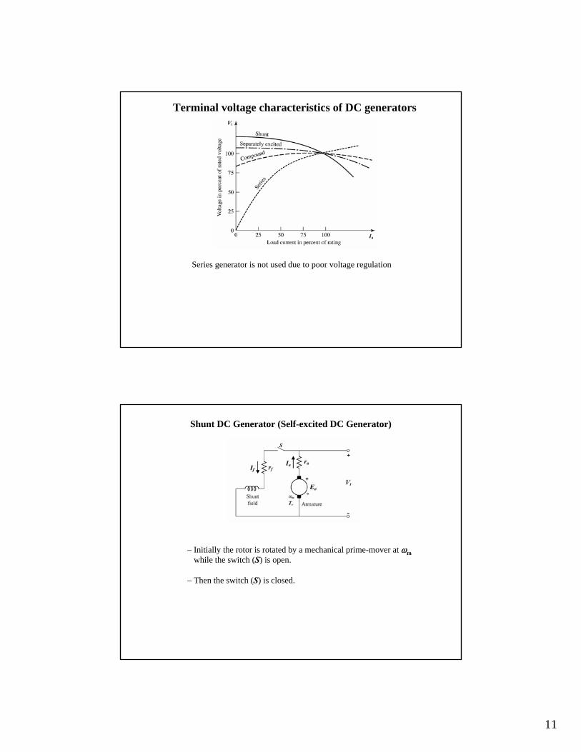
Not used in practical, due to poor voltage regulation
Compound DC Generators
ssaaat rIrIEV +−=mfga KE ωφ=where
LLt RIV =also sL II =and
(a) Short-shunt connected compound DC generator
sf IIIa +=and
15
(b) Long-shunt connected compound DC generator
( )saaat rrIEV +−= mfga KE ωφ=where
LLt RIV =also fIII aL +=and sIIa =and
Types of Compounding
(i) Cumulatively-compounded DC generator (additive compounding)
{ { {
mmf field
series
mmf field
shuntf
mmffield
sd FFF +=
for linear M.C. (or in the linear region of the magnetization curve, i.e. unsaturated magnetic circuits)
sd φφφ += f
(ii) Differentially-compounded DC generator (subtractive compounding)
sd FFF −= f
for linear M.C. (or in the linear region of the magnetization curve, i.e. unsaturated magnetic circuits)
sd φφφ −= f
Differentially-compounded generator is not used in practical, as it exhibits poor voltage regulation
16
Terminal V-I Characteristics of Compound Generators
Above curves are for cumulatively-compounded generators
Magnetization curves for a 250-V 1200-r/min dc machine. Also field-resistance lines for the discussion of self-excitation are shown
17
Examples1. A 240kW, 240V, 600 rpm separately excited DC generator has an armature
resistance, ra = 0.01Ω and a field resistance rf = 30Ω. The field winding is supplied from a DC source of Vf = 100V. A variable resistance R is connected in series with the field winding to adjust field current If. The magnetization curve of the generator at 600 rpm is given below:
310300285260250230200165Ea (V)
65432.521.51If (A)
If DC generator is delivering rated voltage and is driven at 600 rpm determine:a) Induced armature emf, Ea
b) The internal electromagnetic power produced (gross power)c) The internal electromagnetic torqued) The applied torque if rotational loss is Prot = 10kWe) Efficiency of generatorf) Voltage regulation
2. A shunt DC generator has a magnetization curve at nr = 1500 rpm as shown below. The armature resistance ra = 0.2 Ω, and field total resistance rf = 100 Ω.
a) Find the terminal voltage Vt and field current If of the generator when it delivers 50A to a resistive load
b) Find Vt and If when the load is disconnected (i.e. no-load)
18
Solution:
a) b)
NB. Neglected raIf voltage drops
3. The magnetization curve of a DC shunt generator at 1500 rpm is given below, where the armature resistance ra = 0.2 Ω, and field total resistance rf = 100 Ω, the total friction & windage loss at 1500 rpm is 400W.
a) Find no-load terminal voltage at 1500 rpmb) For the self-excitation to take place
(i) Find the highest value of the total shunt field resistance at 1500 rpm(ii) The minimum speed for rf = 100Ω.
c) Find terminal voltage Vt, efficiency η and mechanical torque applied to the shaft when Ia = 60A at 1500 rpm.
19
Solution:
a) b) (i)
b) (ii)
• Series DC motor• Separately-excited DC motor• Shunt DC motor• Compound DC motor
DC motors are adjustable speed motors. A wide range of torque-speed characteristics (Te-ωm) is obtainable depending on the motor types given below:
4. Analysis of DC Motors
20
(a) Series DC Motors
DC Motors Overview
(b) Separately-excited DC Motors
21
(c) Shunt DC Motors
(d) Compound DC Motors
22
(a) Series DC Motors
DC Motors
)( saaat rrIEV ++=
mfga KE ωφ=
sa II =
The back e.m.f:Electromagnetic torque: afge IKT φ=
Terminal voltage equation:
Assuming linear equation: sff IK=φ
)( saaat rrIEV ++=( )fg
saat
fg
am K
rrIVK
Eφφ
ω+−
==
sa II = K
afge IKT φ= sff IK=φ K
2ade IKT =
adfg IKK =φ
asfge IIKKT =
, mfga KE ωφ=K
( )a
saatm KI
rrIV +−=ω afg KIK =φ K
( )saatmada rrIVIKE +−== ω mfga KE ωφ= K
( )samd
ta rrK
VI++
=ω
( )[ ]2
2
samd
tde
rrKVK
T++
=ω
2 ade IKT =K
23
( )[ ]2
2
samd
tde rrK
VKT
++=
ω 21 m
eTω
∝thus
Note that: A series DC motor should never run no load!
∞=⇒→ m 0 ωeT overspeeding!
(b) Separately-excited DC Motors
aaat rIEV +=
mfga KE ωφ=The back e.m.f:Electromagnetic torque: afge IKT φ=
Terminal voltage equation:
Assuming linear equation: fff IK=φ
24
, mfga KE ωφ=K
aaat rIEV +=
fg
aemfgt K
rTKVφ
ωφ += afge IKT φ=
( )2fg
aem
fg
t
KrT
KV
φω
φ+=
( ) efg
a
fg
tm T
Kr
KV
2φφω −=
elm TK−= 0ωω
No load (i.e. Te = 0) speed: fg
t
KV
φω =0
Slope: ( )2fg
al
KrKφ
= very small!
Slightly dropping ωm with load
(c) Shunt DC Motors
aaat rIEV +=
mfga KE ωφ=The back e.m.f:Electromagnetic torque: afge IKT φ=
Terminal voltage equation:
Assuming linear equation: fff IK=φ
25
, mfga KE ωφ=K
aaat rIEV +=
fg
aemfgt K
rTKV
φωφ += afge IKT φ=
( )2fg
aem
fg
t
KrT
KV
φω
φ+=
( ) efg
a
fg
tm T
Kr
KV
2φφω −=
elm TK−= 0ωω
No load (i.e. Te = 0) speed: fg
t
KV
φω =0
Slope: ( )2fg
al
KrKφ
= very small!
Slightly dropping ωm with load
Same as separately excited motor
elm TK−= 0ωω
Note that: In the shunt DC motors, if suddenly the field terminals are disconnected from the power, supply while the motor was running,overspeeding problem will occur
∞→⇒→ m 0 ωφ f
mfga KE ωφ= Ea is momentarily constant, but φf will decrease rapidly.
so overspeeding!
26
Motor Speed Control Methods
Shaft speed can be controlled byi. Changing the terminal voltageii. Changing the field current (magnetic flux)
(a) Controlling separately-excited DC motors
afge IKT φ=
aaat rIEV +=
i. Changing the terminal voltage
elm TK−= 0ωωfg
t
KV
φω =0
↓↓⇒↓ et TV , 0ω
27
afge IKT φ=
ii. Changing the field curerent
elm TK−= 0ωωfg
t
KV
φω =0
↓↑↓⇒↓ eTI , , 0ff ωφ
(linear magnetic circuit)fff IK=φ
Ex1: A separately excited DC motor drives the load at nr = 1150 rpm.
a) Find the gross output power (electromechanical power output) produced by the dc motor.
b) If the speed control is to be achieved by armature voltage control and the new operating condition is given by:
nr = 1150 rpm and Te = 30 Nmfind the new terminal voltage V′t while φf is kept constant.
28
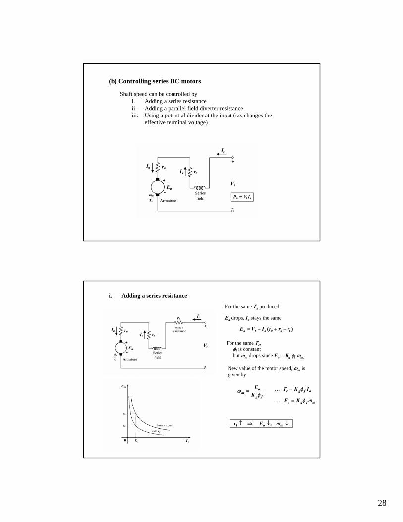
Shaft speed can be controlled byi. Adding a series resistanceii. Adding a parallel field diverter resistanceiii. Using a potential divider at the input (i.e. changes the
effective terminal voltage)
(b) Controlling series DC motors
i. Adding a series resistance
)( tsaata rrrIVE ++−=
fg
am K
Eφ
ω = afge IKT φ= K
Ea drops, Ia stays the same
For the same Te, φf is constant
but ωm drops since Ea = Kg φf ωm..
New value of the motor speed, ωm is given by
mfga KE ωφ= K
, r mt ↓↓⇒↑ ωaE
For the same Te produced
29
ii. Adding a parallel field diverter resistance
fg
am K
Eφ
ω =sff IK=φ K
Is drops i.e. Is < Ia.
Ea remains constant,
When series field flux drops, the motor speed ωm = Ea / Kg φf should rise, while driving the same load.
mfga KE ωφ= K
, , , r mfd ↑↓↑↓⇒↓ ωφas II
For the same Te produced, Ia increases
)||( dsa
ata rrr
EVI
+−
= sds rrr || <K
When we add the diverter resistance
iii. Using a potential divider
This system like the speed control by adding series resistance as explained in section (i) where rt ≡ RTh and Vt ≡ VTh.
tTh VRR
RV21
2
+=
Let us apply Thévenin theorem to the right of V′t
21 || RRRTh =
)( ThsaaTha RrrIVE ++−=
fg
am K
Eφ
ω = afge IKT φ= K
Ea drops rapidly, Ia stays the same
For the same Te, φf is constant
but ωm drops rapidly since Ea = Kg φf ωm..
mfga KE ωφ= K
, V mt ↓↓↓↓⇒↓′ ωaE
For the same Te produced
New value of the motor speed, ωm is given by
If the load increases, Te and Ia increases and Ea decreases, thus motor speed ωm drops down more.