APPLICATION OF THE METHODS OF QUANTUM FIELD THEORY 299

and hence

~ a~ evL = tX+ (eaLJav _ 1) evL. (A.28)

By comparing Eq. (A.28) with (A.26), we obtain the desired relation between L and a' ,

aa' (v) I a"V = eaLJov - 1. (A.29)

Equations (A.29) and (A.25) imply Eq. (A.15), and by Eq. (A.24) this proves Eq. (A.14).

1V. B. Berestetskii and A. D. Galanin, IIpooJieMhi

coBpeMeuuoii <f>n3HKH (Problems of Modern Phys­ics), No. 3 (1955), (introductory paper). - 2 Abrikosov, Landau, and Khalatnikov, Dokl. Akad. Akad. Nauk SSSR 95, 497, 773 and 1177; 96, 261 (1954).

3 v. M. Galitskii and A. B. Migdal, J. Exptl. Theoret. Phys. (U.S.S.R.) 34, 139 (1958); Soviet Phys. JETP 7, 96 (1958).

4 F. J. Dyson, Phys. Rev. 75,1736 (1949). 5 N. N. Bogoliubov, Izv. Akad. Nauk SSSR, ser.

fiz. 11, 77 (1947). 6 s. T. Beliaev, J. Exptl. Theoret. Phys. (U.S.S.R.)

34, 433 (1958); Soviet Phys. JETP 7, 289 .(1958) (this issue).

7 G. C. Wick, Phys. Rev. 80, 268 (1950). 8 R. P. Feynman, Phys. Rev. 76, 749 (1949). 9 S. Hori, Prog. Theoret. Phys. 7, 578 (1952).

Translated by F. J. Dyson 77

SOVIET PHYSICS JETP VOLUME 34 (7), NUMBER 2 AUGUST, 1958

ENERGY-SPECTRUM OF A NON-IDEAL BOSE GAS

S. T. BELIAEV

Academy of Sciences, U.S.S.R.

Submitted to JETP editor August 2, 1957

J. Exptl. Theoret. Phys. (U.S.S.R.) 34, 433-446 (February, 1958)

The one-particle Green's function is calculated in a low-density approximation for a system of interacting bosons. The energy spectrum of states near to the ground state (quasi-particle spectrum is derived.

1. INTRODUCTION

IN the preceding paper1 the method of Green's functions was developed for a system consisting of a large number of bosons. The one-particle Green's function was expressed in terms of the effective po­tentials l::ik of pair interactions and the chemical potential J.l of the system. Approximate methods must be used to determine l::ik and J.l. In the present paper we study a "gaseous" approximation, in which the density n, or the ratio between the volume occupied by particles and the total volume, is treated as a small parameter. The interaction between particles is assumed to be central and short-range, but not necessarily weak. The first two orders of approximation involve only the scat­tering amplitude f of a two-particle system. But in the. next order (proportional to ( -.fnfS )2 ) the effects of three-particle interaction amplitudes

appear, which means that practical calculations to this order are hardly possible.

From the Green's function which we calculate, we derive the energy spectrum of excitations or quasi-particles, the energy of the ground state, and also the momentum distribution of particles in the ground state.

2. ESTIMATE OF THE GRAPHS CONTRIBUTING TO THE EFFECTIVE POTENTIALS

The definition of the potentials .l::ik• and the rules for constructing Feynman graphs, were de­scribed in our earlier paper, 1 which we shall call I.

We shall estimate by perturbation theory the various graphs contributing to l::ik and J.l. For the Fourier transform of the potential U (p) =Up,

300 S. T. BELIAEV

we assume for simplicity* Up= U0 for p < 1/a, and Up= 0 for p > 1/a. Then a is of the order of magnitude of the particle radius.

For definiteness we examine ~20 • The graphs for ~02 , ~ 11 and J.1. are essentially similar. The first order of perturbation theory, as we saw in Sec. (1,7), gives ~~~)= noUp; J.1. =noVo.

In the estimate of any graph there may appear three parameters - U0 and a, characterizing the interaction, and no. characterizing the density of particles in the condensed phase. The three pa­rameters can be combined into two dimensionless ratios,

~ = V n0a3• (2.1)

The quantity ~ is the usual parameter which ap­pears in perturbation theory (in ordinary units ~ ~ m U ( r) a2/n 2 ), while {3 is a parameter of gas-density.

t~f t_----{ 'J~I=fz l _ _j a --- 4

a 11

FIG. 1 FIG. 2

The only noli-vanishing graph in second order is the one shown in Fig. 1a. This gives a contri­bution

Ma~n0 ~ 0° (q +fl.) 0° (-q +fl.) U0Up+qd4q

Substituting for G0 from

QO(p)=(pO-eO+iop, eO=p2 j2, p p 0---++0 (2.2)

and carrying out the q0 -integration, we find

In the last integral the main co11tribution comes from q ~ 1/a, where JJ./E0 ,.... n0U0a2 = ~{32 « 1. Therefore

(2.3)

We consider next the third-order graph (1b). This gives a contribution

*The letters p, q, • • . are used to denote the lengths of 3-vectors, or to denote 4-vectors. There can be no confusion, because they denote 4-vectors only when they appear as argu­ments in G(p), .:£(p), etc.

Mb ~ n~~ 0° (q +fl.) [0° (- q + (1.)]2 U0UqUp+qd4q

~ n~U~ ~dqf(fl.-s~ + io)2 •

The last integral, unlike the previous one, con­verges at the upper limit, and the main contribu­tion now comes from the range q ~ {ji = v'nou0 •

Therefore

M 2ua 1 ,;- ~<I>· •t,~ b ~ no o v fl. = "-'20 ~ t'· (2.4)

From Eqs. (2.3) and (2.4) we see that M0/Ma ~ ~ 112{3. This is a consequence of the fact that Ma contains an integral of a product of two factors G0,

formally diverging at the upper limit, while Mb contains an integral of a product of three factors G0 and converges without any cut-off. In the graphs this difference is indicated by the number of continuous lines in the closed circuit formed by the continuous and dotted lines. The same result holds when the circuits form part of a more com­plicated graph.

Thus every circuit containing more than two continuous lines introduces the small parameter {3, while circuits with two continuous lines do not in­volve {3. In the lowest order we need consider only graphs whose circuits are all of the two-line type. All such graphs are of the "ladder" construction shown in Fig. 2. We denote by - ir ( 12; 34) the total contribution from all such graphs. The first­order approximation in {3 then differs from the first-order approximation in perturbation theory by changing the potential U ( arising from a ladder with one rung) into r (arising from ladders of all lengths ) . Similar conclusions hold also for the higher approximations. A summation over a set of graphs, differing only by the insertion of ladder circuits into a fixed skeleton, produces a change of U into r. If we represent r by a rectangle, a.ll graphs can be constructed by means of rec­tangles and continuous lines only. In this way the potential U is eliminated from the problem. The effective potential is r.

3.* EQUATION FOR THE EFFECTIVE POTENTIAL r

We can write down an integral equation

r (12;34) = u (1-2) o (1-3) o (2-4)

+ i ~ u (1-2) G0 (1-5) G0 (2-6) r (56; 34) d4x5d4x6. (a.1)

for the sum of contributions from a.ll graphs of the ladder type (see Fig. 2). The notations are the

*The problems connected with [' were solved in collabora­

tion with V. M. Galitskii, who was working simultaneously on the analogous problems in Fermion systems.

ENERGY-SPECTRUM OF A NON-IDEAL BOSE GAS 301

same as in I. We next transform Eq. (3.1) into momentum representation. In order to relieve the equations of factors of 27!", we shall use the con­ventions

d4p = (21tf'dp1dp2dp3dp0 ;

a (p) = (21t)' a (pl) a (p2) a (ps) a (po),

and similarly we understand dp and 6 ( p) to carry factors of ( 27!" )3• We write

f (p1P2; PaP4) a (PI + P2- Pa- P4)

= ~ exp {- ip1x1 - ip2x2 + ipaXs (3.2)

+ ip4x4} r (12; 34)d4xld4x2d4xad4x4,

and introduce the relative and total momenta by

P1 + P2 = P'; Ps + P4 = P;

P1- P2 = 2p', Pa- P4 = 2p, (3.3)

Then, by Eq. (3.1), r(p'; p; P) = r(PtP2; PaP4) satisfies the equation

r (p'; p; P) = u (p'- p) + i ~ d4qU (p'- q) ao (P/2 + q)

X G0 (P/2- q) r(q; p; P). (3.4)

Since the interaction U is instantaneous, U ( 1 - 2 ) = U ( x 1 - x2 ) 6 ( t 1 - t2 ) , and therefore the points 1, 2 and 3, 4 in r ( 12; 34) must be simultaneous. In momentum representation this means that r ( p1 p2 ; p3 p4) depends on the fourth components only in the combination p~ + p~ = p~ + p~ = P0• Therefore r ( p'; p; ·p) is independent of the fourth components of its first two arguments (the relative momenta). The q0-integration in Eq. (3.4) can thus be carried out, giving

~ dqOGO (} p + q) GO ( + p- q) ( 1 )-1 = - i \ po- 4 p2- q2 + ia '

and then Eq. (3.4) takes the form

f (p'; p; P) = U (p'- p) + \ dq U (P~2- q): (q::; P) .\ 0-q +l

k2 _ po _ ..!_ p2 0- 4 •

(3.5)

(3.6)

Equation (3.6) cannot be solved explicitly, but its solution can be expressed in terms of the scat­tering amplitude of two particles in a vacuum. We write x(q)=(k~-q2 +.i6)- 1 r(q;p;P). Then Eq. (3 .6) becomes

(k~- p'2)x (p')- ~ U (p'- q) X (q) dq = U (p'- p). (3.7)

Let ..Yk ( p') be the normalized wave-function which satisfies the equation

w- p'2) 'Yk(p')- ~ u (p'- q) 'Yk (q) dq = 0, (3.8)

Then the solution of Eq. (3.7) may be written

, ('Yk (p') 'f'; (q) u ) d X(P)= .\ k;-k2+i3 (q-p q,

and so r ( p'; p; p) becomes

f{ '· ·P)=(k2 - ' 2)\ Tk(p')'f';(q) U(- )d (3.9) p 'p, 0 p .\ k~- k2 + i3 q p q.

We observe now that Eq. (3.8) is the Schrodinger equation in momentum representation. Thus ..Yk ( p) is the wave-function for a scattering problem with potential U. The scattering amplitude* f ( p' p) is related to the ..Y-function by

f (p'p) = ~ e-ipr U (r) Wp (r) dr = ~ U (p'- q) Wp (q) dq, (3.10)

or by

wp (p') =a (P- p') + f (p'p)/(P2 - p'2 + ia). (3.11)

In the first Eq. (3.10), ..Yp (r) is the wave-function in coordinate. space which behaves at infinity like a plane wave with momentum p and an outgoing spherical wave. The usual scattering amplitude is the value of f (p' p) at p' = p. We consider arbi­trary values of the arguments, so that f ( p' p ) is in general defined by Eq. (3.10).

Because ..Yp ( p') satisfies orthogonality condi­tions in both its arguments, f ( p' p ) satisfies the unitarity conditions

t (p'p) - r (p'p)

= ~dqf(p'q)f"(pq)[q•-:'2+i3- q2_;2-i3l

= ~ dqf" (qp') f (qp) [q2- ;,2 + i3 - q2- p;- i3 J. (3.12)

When p' = ±p, Eq. (3.12) gives the imaginary part of the forward and backward scattering amplitudes. Since f ( -p'- p) = f (p' p ), Eq. (3.12) implies

Im f (± pp) = ·- i1t ~ dqf (pq) f" (+ pq) a (q2 - p2). (3.13)

For the forward scattering amplitude, Eq. (3.13) gives just the well-known relation between the imaginary part of the amplitude and the total cross­section a, Im f ( p p ) = - ipa.

We substitute Eq. (3.11) into (3.9) and use Eq. (3.12). This gives two equivalent expressions for r (p'; p; P ),

r (p'; p; P) = t (p'p)

+ ~ dqf (p'q) r (pq) [ kg-q• ~ n~ + ,q2-p!-ia] (3.14)

= r (pp') + ~ dqf (p' q) r (pq) [ k~ _ ~. + ia + q2 _ ~~2 + i3] ·

*The quantity f(p' p) differs by a numerical factor from the usual amplitude a (p' p), in fact f = - 4 n a.

302 S. T. BELIAEV

expressing the effective potential r ( p'; p; P) in terms of the scattering amplitudes of a two-parti­cle system.

4. FIRST-ORDER GREEN'S FUNCTION

The effective potentials 1: ik are determined by special values which r takes when two out of the four particles involved in a process belong to the condensed phase. Thus two of the four particles must have p = 0, p0 = J.L. Each particle of the con­densed phase also carries a factor ~ . There­fore we find

E20 (p + fL) = n0r (p; 0; 2[L); E02 (p + fL) = n0r (0; p; 2[L),

E11 (p + f.l) = n0r (pj2; pj2; p + 2[L) (4.1)

+nor (- pj2; pj2; p + 2[L).

To obtain the chemical potential we must let all four particles in r belong to the condensed phase, and divide by one power of n0 [see Eq. (I, 3.20)]. We then have

(4.2)

Substituting into Eqs. (4.1) and (4.2) the value of r from Eq. (3.14), we find

[L = nof (00) + no ~ dq i f (Oq) 1,2 [ 21L _

1q• + i8 + ;. ] ' !:2o (p + fL) = nof (pO)

+ n0 ~ dqf (pq) f'(Oq) [ 2!'- _ 1qz + i8 + :. ] • E02 (p + fL) = nof" (pO)

+ no~ dq f (Oq) f* (pq) [2!'- _ ~. + i8 + :.l ~u (p + fL) = 2nofs(++)

+ 2no ~ dq If s ( ~ q) n pO + 2!'-- p~/4- q• + i8

(4.3)

In the last equation we have introduced the sym­metrized amplitude

f s (p'p) = If (p'p) + f (- p'p)]/2.

All the integrals in Eq. (4.3) converge at high momentum, even if the amplitudes are taken to be constant. For dimensional reasons these terms are of order nof2 ..fjj:. Compared with the first terms in Eq. (4.3), these terms contain an extra factor ..fDJf", which is just the gas-density param­eter (2.1) obtained by substituting the amplitude f for the particle radius. In first approximation we neglect the integral terms in Eq. (4.3) and obtain

f! = n0f (00); E20 (p + f.l) = E~z (p + [L) = nof (pO); (4.4)

The Green's function G is given by Eq. (I, 5.6),

G (p + !-') pO + €~ + LU: - fl.

(p"- (Li;:- LU:)/2]2- (o~ + (Li;: + Lti)/2- !LJ2 + L 20L 02 + i8

(4.5)

and after substituting from Eq. (4.4) this becomes

p0 + o0 + 2n0f s (_ll_ __p_ \- n0f (00) G ( + ) . 2 2 J (4.6) p f.l = 02 2 ' ·~ ,

p -E~ T to

with

Cp = Jlls~ + 2nofs( ++)-not (00) r- n~ If (pO) 12 • (4.7)

The point Po ( p ) , at which the Green's function G (p + J.L) has a pole, determines the energy Ep of elementary excitations or quasi-particles2 car­rying momentum p. To calculate Ep we must know three distinct amplitudes. fs (p/2 p/2) is the ordinary symmetrized amplitude for forward scattering, and f ( 0 0) is a special value of the same amplitude. However, f (p 0) does not have any obvious meaning in the two-particle problem, since it refers to a process which is forbidden for two particles in a vacuum.

At small momenta, we may neglect the momen­tum dependence of fs (p/2 p/2) and of f (p 0 ), setting fs (p/2 p/2) ·~ f (p 0) ~ f ( 0 0) = f0•

This approximation is allowed when the wavelength is long compared with the characteristic size of the interaction region, which has an order of mag­nitude given by the scattering ampfitude f0• There­fore when p < f01 we may consider all the ampli­tudes in Eq. (4.6) and (4.7) to be constant. For higher excitations with p ~ f01, the momentum dependence of the amplitude becomes important, and the problem cannot be treated in full generality. We shall examine the higher excitations (in Sec. 8) for the special example of a hard-sphere gas.

Confining ourselves to the case pf0 < 1, we de­duce from Eq. (4.6) and (4. 7)

G (p + !L) = (p0 + s~ + n0f0)/(p02 - s~ + i8), (4.8)

with

(4.9)

Equations (4.8) and (4.9) are formally identical with the results obtained from perturbation theory in Eq. (I, 7 .3) and (I, 7 .4). Only the scattering am­plitude f0 now appears instead of the Fourier transform Up of the potential.

Equation (4.9) shows that quasi-particles with p « .Jn0f0 have a sound-wave type of dispersion law E Rl p .Jn0f0 • When p » .Jnofo they go over into :ifmost free particles with Ep R~ E~ + n0f0•

ENERGY-SPECTRUM OF A

This sort of energy spectrum appears also when one considers particles moving in a continuous medium with a refractive index. The transition from phonon to free particle behavior occurs at p ~ -./n0f0 « 1/f0, so that the approximation of constant amplitudes is valid in both ranges.

The conditions -./n0f~ « 1 and pf0 « 1 are not independent. If we look at momenta p not greatly exceeding -./n0f0 , then the second condi­tion is a consequence of the first. If we are then neglecting quantities of order -./n0fij , we must also treat the amplitudes as constant.

In Sec. (I, 5) we introduced the quantity <1 ( p + JL), the analog of the Green's function G but constructed from graphs with two ingoing ends instead of one ingoing and one outgoing. The analo­gous quantity with two outgoing ends will be denoted by G ( p + JL ) . It is obtained from G ( p + JL ) when 1:02 is replaced by 1:20 • In the constant-amplitude approximation, Eq. (I, 5. 7) and (4.4) give

G (p +fl.) = G (p +fl.) =- n0f0f(p02 - s~ + i8). (4.10)

5. SECOND APPROXIMATION FOR THE GREEN'S FUNCTION

For the second approximation to ~ and JL, we must retain quantities of order v'n0fg . As we saw at the end of the preceding section, we must then also retain terms of order pf0 in the ampli­tudes. The real part of the amplitude involves only even powers of p, and the imaginary part only odd powers. Terms of order pf0 arise only from the lowest approximation to the imaginary part of the amplitudes. The imaginary part of fs (p/2 p/2) is given by Eq. (3.13), and from Eq. (3.10) we see that the amplitude f ( p 0 ) is real [and anyway in this approximation we need only the square of the modulus of f (p 0 )].

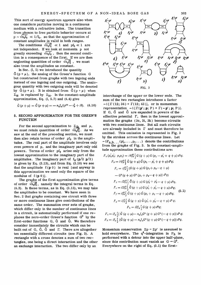
The graphs of the first approximation give terms of order -./n0f8, namely the integral terms in Eq. (4.3). In these terms, as in Eq. (3.13), we may take the amplitudes to be constant. We have seen in Sec. 2 that graphs containing one circuit with three or more continuous lines give contributions of the same order. The summation over sets of graphs, which differ only in the number of continuous lines in a circuit, is automatically performed if one re­places the zero-order Green's function G0 by the first-order functions G, G and G. We therefore consider immediately the circuits which can be built out of G, G, G and r. There are altogether ten essentially different circuits (see Fig. 3). A rectangle with a cross denotes a sum of two rec­tangles, one being a direct interaction and the other an exchange interaction. The two differ only by an

interchange of the upper or the lower ends. The sum of the two rectangles introduces a factor - i [ r ( 12; 34) + r( 12; 43 )], or in momentum representation - i [ r(p'; p; P) + r(-p'; p; P )] . If G, G and G are expanded in powers of the effective potential r' then in the lowest approxi­mation the graphs ( 3c, 3i, 3k) become circuits with two continuous lines. But all such circuits are already included in r and must therefore be omitted. This omission is represented in Fig. 3 by the strokes across the continuous lines. Let - iF a ,b ... (Pi, ... , P1 ... ) denote the contributions from the graphs of Fig. 3. In the constant-ampli­tude approximation these contributions are:

Fa (p~p~; PrP2) = i4f~ ~ G (q +fl.) G (Pr- p~ + q +fl.) d4q;

Fb = i4f~ ~ G (q +fl.) G (p1 - p~ + q + fl.}d4q;

Fe= in~ {G (q +fl.) G (Pr+ P2-q + !L)

- 0° (q +fl.) G0 (Pr + P2- q +fl.)} d4q;

Fd = i2n ~ G (q +fl.) G (p; + p;- q + !L)d4q,

F, = i2n ~a (q + !L) a (p~ + p~ _ q + !L) d4q;

Ff =if~~ G (q +fl.) G (Pr + P2- q +fl.) d4q;

F g =if~) G (q + p.) G (p~ + p~- q + !L) d4 q;

F h = i2f 0 ~ G (q +fl.) d4q;

(5.1)

F i =if 0 ~ { G (q + !L)- nof oG0 (q + !L) 0° (- q + p.)} d4 q;

Fk = ifo ~ {G (q +fl.)- n0{ 0G0 (q + !L) 0° (- q +fl.)} d4q.

Momentum conservation 1:p = 1:p' is assumed to hold everywhere. The q0-integration in Fh is performed with a detour into the upper half-plane, since this contribution must vanish as G - G0•

Everywhere on the right of Eq. (5 .1) the first-

304 So To BELIAEV

approximation value J.L( 1) = n0f0 should be substi­tuted for J.Lo

The ~ik involve special values of the F, to­gether with a factor ..fllo for each particle of the condensed phase:

E~o (p + p.) = n0F a (p- p; 00)

+n0Fb(p-p; 00) +n0Fe(p0-p; 0)

+ n0Fe (Op- p; 0) + n0Fe (-pOp; 0)

+ n0Fe (0- pp; 0) + n0F g (pO- pO;)

+ n0F g (pOO-p;)+ F; (p- p;);

E~2 (p + fL) = n0Fa (00; p- p)

+noFb(OO; p-p)+noFd(O; p-pO)

+ n0F d (0; pO - p)

+ n0F d (0; - ppO) + n0F d (0; -pOp)

+ n0FJ (; pO- pO)

+ n0FJ (; pOO-p)+ FR.(; p- p);

E~1 (p + fl.) = n0F a (pO; Op) + n0F b (pO; Op)

+ noFc (pO; pO) + n0Fc (pO; Op)

+ n0F d (p; OpO) + n0F d (p; OOp)

(5.2)

+ noF.(pOO; p)+n0F.(Op0; p) + Fh(p; p).

To enumerate the vacuum loops which contribute to J.L, we must first distinguish one incoming or outgoing particle of the condensed phase (see Sec­tion (1, 4)) 0 After this we must sum the loops, counting separately all possible geometric struc­tures and all possible positions of the distinguished particle 0 The vacuum loops include three types of rectangle, differing in the numbers of incoming and outgoing continuous lines, and corresponding to fac­tors ~H>, ~AP and ~W 0 The distinguished parti­cle of the condensed phase may come out from ~ H> or from ~ ~p 0 The sums of contributions from graphs of these two types are respectively -iFh(O; 0) and -iFi(O O;)o The term in J.L

arising from all these vacuum loops is thus

fL' = Fh(O; 0) + Fi(OO;)o (5.3)

To carry out the q0-integration in Eq. (5.1), it is convenient to represent G and G = G in the following form,

Aq G{q+p.) = qo-e +i8

q

= -C [ 1 _ 1 ] .q qo- E + i8 q0 + E - i8 ' q q 0

(5.4)

with

Aq = (sq + z~ + nofo) / 2sq;

Bq = (- sq + s~ + n0f 0) I 2sq

= nU~ I 2sq ( sq + s~ + n0 fo}; Cq = n0f 0 / 2sq (5.5)

depending only on jqjo The q0-integrations are now performed and the results substituted into Eq. (5.2) and (5.3). After some manipulations we ob­tain

E~2 <2o> (p +fl.) = 2non ~ dq [(Aq; Bk)

- (Aq + Bq; Ck) + 3CqCk]

f \ d fC + nofo l - 0 ~ q 1 q 2n0f0 - 2e~ + i8 { '

_ (Aq; Bk) + 2CqCk + BqBk- 2 (Bq; Ck)

pO + Eq + Ek- i8 (5 o6)

Here k = p - q, and the symbol (;) denotes a symmetrized product, (Aq; Bk) = AqBk + BqAko The integrands are all symmetrical in q and ko

Before we add to Eq. (5.6) the second-order terms from Eq. (4.2), we transform the expression (4o3) for ~ 11 0 Remembering'that

and introducing the new integration variable q' = q + p/2, we find that Eq. (4.3) gives to the required approximation

En (p + fl.) = 2n0f 0 + 2n0 Im f s ( f f) + 2nof~ \ dq [ 1

0 0 ~ po+2n0f0 -eq-ek+i8

(5.7)

The total of all second-order terms in now obtained from Eq. (5.6), (4.3), and (5.7), and after some pl­gebra becomes

ENERGY-SPECTRUM OF A NON-IDEAL BOSE GAS 305

fL< 2> = 2f 0 ~ dq Bq + { nof~ ~ dq ( e~ - :q) •

l:~~><o2> (p + f.l) = 2non ~ dq [(Aq; Bk)

- (Aq + Bq; Ck) + 3CqCk]

1 1 X (po- eq- ek + ill - p" + eq + ek- ill)

+ {-non ~ dq ( :~ - :q ) ;

Eii> (p + f.l)

(5 .8)

+ 2n0 Im f s ( f f) - 2n f2 ~ d [ 1 _j_ _1 __!_] o o q o o o + ·~ ' 4e + 4e ' ep- eq- ek !o q k

The value of Im fs (p/2 p/2) can be obtained from Eq. (3.13), and the integrals not involving p0 can be carried out exactly. In this way Eq. (5 .8) be­comes

(5.9)

(5 .10)

(5.11)

with

R (qk) = 2s~sg- 2sqsk + n~f~, Q" (qk) = 3s~eg- sqsk + n0f 0 (eg + e~) + + nM~+ [n0{ 0 (sq + sk)- sqs~- ekeg}. (5.12)

(

It is convenient to express the Green's function (4.5) in a form analogous to Eq. (5 .4). In this ap­proximation we find

A +rx G (p + f.l) = P P -

p"-eP-AP (5.13)

where O!p and A~ are the second-order correc­tions

+ e~ + - (2) Ap = z~ (En+ En- 2f.l) +

-p

nofo ("+ .,- 2 2., )(2) 1 ("+ "'-)(2) + ~ "-'n + "-'n- fL - "-'2o + 2 "-'n- "-'n · p

(5.14)

These O!p and A~ are combinations of the in­tegrals (5.9) and (5.10). In the limits of small and large momentum (compared with .../nofo ), explicit expressions can be obtained for the functions O!p = a (p0; p) and A~= A'F(p0; p). When these are ex­amined it is found that there are no new poles of the Green's function. We here exhibit the behavior of the Green's function near to the poles Po Rl ± Ep .

In this region we may write jp0 j = Ep in O!p, and we need retain only terms of first order in the dif­ference ( Ep 'F p0 ) in A~. For small momenta ( p « .../n0f0 ) we then find

V-f3( 2 nofo . 1 ep ) rxp= no o 32- + ~~-~ IT Ep IT no 0

For large momenta only the imaginary part of A~ is important,

(5 .16)

For small momenta, in virtue of Eq. (5.13) and (5.15), the Green's function near to the poles may be written in the form

(5 .17)

For large momenta, O!p and ::\p may be neg­lected in Eq. (5.17).

6. QUASI-PARTICLE SPECTRUM AND GROUND-STATE ENERGY

We have already mentioned that the energy of a quasi particle is determined by the value of p0 (p) at a. pole of G ( p + p,). Only those poles are to be considered for which the imaginary part of the en­ergy is negative, so that the damping is positive. In the range p « .../n0f0 , Eq. (5 .15) and (5 .17) give

s = p V nof o ( 1 + 6:2 V non)

. 3 v-3 p• v-- 16-40 nofo --,1 (p<Z; nofo),

IT (nof ol 2 (6.1)

306 S. T. BELIAEV

In the high-momentum range, according to Eq. (5.16), we have

+ nof (pp) (p c';s> v nof o)· (6.2)

Equation (6.1) shows that for small p the quasi particles are phonons. The second approximation gives a correction to the sound velocity, and a damping proportional to p5 which is connected with a process of decay of one phonon into two. In the high-momentum range, the second approxima­tion gives a damping which is related to the imagi­nary part of the forward scattering amplitude, and so to the total cross section.

In Sec. (I, 7) we found connections between the Green's function and various physical properties of the system. The mean number of particles Np with a given momentum p in the ground state of the system is related to the residue of the Green's function at its upper pole,

Np = i ~ G dp0 / 2<- = (Bp + cxp) (I- Ap)· (6.3)

When p « -./n0f0 , Eqs. (5.15) and (5.5) give

(6.4)

The imaginary parts of ap and A.p here cancel, as they should. To find the total number of parti­cles with p 'J'!. 0, we need to lmow Np for all mo­menta. We therefore use only the first approxima­tion formula for Np, namely Np = Bp. For the density of particles with p 'J'!. 0 we find

n-n0 = i ~ G (p + 11-)d4 p

(6.5)

Equation (6.5) gives the relation between the den­sity n0 of particles in the condensed phase, which appeared as a parameter in all our equations, and the total number of particles in the system.

We note here one important point. It can be seen from the way the calculations were done that the validity of the "gaseous" approximation re­quires that n0 be small. It is not directly required that the total density n be small, since n does not appear explicitly in the problem. But Eq. (6.5) shows that when n0 is small n is necessarily small, too. This means that it is not possible to decrease significantly the density of the condensed phase by increasing the interaction or the total density, so long as n0 « f03• This result confirms and strengthens the assertion made in I that the

condensed phase does not disappear when interac­tions are introduced.

We can calculate the ground-state energy from the chemical potential p,. By Eq. (4.4) and (5.11),

11- = nofo I+ 3rt2- V nofo , ( 5 -3) (6.6)

Expressing n0 in terms of n by means of Eq. (6.5), we have in the same approximation

· 4 v-a) iJ.= nfo(l+ 3rt2 nfo.

(6. 7)

By definition we have J.L = aan ( ~0 ). Therefore,

integrating Eq. (6.7) with respect to n, we obtain the ground -state energy

Eo _ ~ 2 ( J!!_ ,-3

v - ~ n f o \I + 15rr2 V nf o) ' (6 .8)

This coincides with the result of Lee and Yang3

for the hard-sphere gas, if we remember that in that case f0 = 47ra.

The condition for the system to be thermody­namically stable is BP/av = -B2E/av2 < o. This condition reduces to f0 > 0. Our results are only meaningful when this condition is satisfied.

7. POSSIBILITY OF HIGHER APPROXIMATIONS

In the first two approximations, all the results can be expressed in terms of the amplitudes f. Thus the problem of many interacting particles is reducible to the problem of two particles.

a b

FIG. 4

In the next approximation we must consider con­tributions to I:ik proportional to n0f~. Among other graphs, we must include the "triple ladders" illustrated in Fig. 4. The integrals arising from graphs of this type diverge at high momenta and become finite only when the momentum dependence of f is taken into account. For an estimate we may cut the integrals off at a momentum p ~ f01•

We see then that an increase in the number of "rungs" does not change the order of magnitude of the integral. In fact, each rung adds a factor f0G2 and an integration over one momentum 4-vector. For a rough estimate we take q0 ~ q2, G ~ q-2, and find

ENERGY-SPECTRUM OF A NON-IDEAL BOSE GAS 307

~ f o02d4q~ f 0 ~ dq ~ I'

Therefore we have to consider simultaneously all such graphs with any number of rungs. The total­ity of these triple ladders describes completely the interaction of three particles. Therefore the sum of contributions from such graphs can be expressed only by means of three-particle amplitudes.

In the third approximation (terms proportional

to n0f~) we thus require a solution of the three­particle problem (see also Ref. 4). Since the problem of three strongly interacting particles is in general insoluble, the higher approximations to the many-particle problem are physically mean­ingless.

8. HIGH EXCITATIONS (pf0 ,..., 1) IN A HARD­SPHERE GAS

For the high-energy excitations, the momentum dependence of the amplitudes becomes important. We therefore consider as an example the case of a gas of hard spheres of radius (a/2 ). We also consider only the first approximation in the den­sity expansion, i.e., we use Eq. (4.6). The ampli­tude f (p 0) can be computed exactly from Eq. (3.10). For fs (p/2 p/2) we consider only s­waves. The higher waves (the symmetrized am­plitude involves only even values of P.) add a numerically unimportant contribution. For exam­ple the d-waves at pa ~ 1 contribute about 10 per cent. We substitute into Eq. (4.7) the values of the amplitudes

f ( 0) _ 4_ sin pa • f ( p p) _ 8T: . pa -ipa 12 p - "-- , s I -.:;- -2 - - Sin -c; e · , p \- p ~

(8.1)

and obtain for the quasi-particle energy

[( p2 sin pa \ 2 2 9 sin 2 pa]"' s = T + 8r.:n 0 -P--- 4rrn0a) - !61t n0 ~ , (8.2)

At high momenta this becomes

(8.3)

The second term in Eq. (8.3) changes sign at pa ~ 1. 9. An oscillating component is superim­posed on the usual parabolic dependence. This oscillation will not be important since the magni­tude of the term is small; when pa "' 1 it is of relative order n0a 3 • However, if one formally allows the parameter n0a3 to become larger in Eqs. (8.3) or (8.2), the second term of Eq. (8.3) produces an increasing departure of the disper­sion law from the parabolic form, until at suffi­ciently high densities there appears first a point of inflection and finally a maximum and a mini-

mum in the curve. The spectrum then resembles qualitatively the spectrum postulated by L. D. Landau5 to explain the properties of liquid helium II. This extrapolation is certainly unwarranted. But it allows one to suppose that the difference between liquid helium and a non-ideal Bose gas is only a quantitative one, and that no qualitatively new phenomena arise in the transition from gas to liquid.

9. CONCLUSION

We summarize the main features of the approx­imation which we have studied.

(1) The interaction between particles is specified not by a potential but by an exact scattering ampli­tude. This allows us to deal with strong interac­tions. After the potential has been replaced by the amplitude, it is possible to make a perturbation ex­pansion in powers of the amplitude, or more pre­cisely in powers of v'n0f~ .

(2) We make a series expansion not of the quasi­particle energy (this appears as the denominator of the Green's function), but of the effective inter­action potentials ~ and the chemical potential J.L.

The formula giving the Green's function in terms of 1: ik and J.L is exact.

From Eq. (4.7) and (4.9) we see that Ep can be expanded in powers of f only for high-momentum excitations with p » v'nof0 • The low-lying excita­tions of the system are in principle impossible to obtain by perturbation theory. For this reason, the expression obtained by Huang and Yang4 for the energy of the low excitations of a Bose hard-sphere gas is incorrect. They used perturbation theory with a "pseudopotential ," and their result agrees with a formal expansion of Eq. (4.7) in powers of fo.

In conclusion I wish to thank A. B. Migdal and especially V. M. Galitskii for fruitful discussions, and also L. D. Landau for criticism of the results.

1s. T. Beliaev, J. Exptl. Theoret. Phys. (U.S.S.R.) 34, 417 (1958); Soviet Phys. JETP 7, 289 (1958) (this issue).

2 V. M. Galitskii and A. B . Migdal, J. Exptl. Theoret. Phys. (U.S.S.R.) 34, 139 (1958); Soviet Phys. JETP 7, 96 (1958).

3 T. D. Lee and C. N. Yang, Phys. Rev. 105, 1119 (1957).

4 K. Huang and C. N. Yang, Phys. Rev. 105, 767 (1957).

5 E. M. Lifshitz, Usp. Fiz. Nauk 34, 512 (1948).

Translated by F. J. Dyson 78