Validation of Gyratory Mix Design in Iowa Final Report July 2016 Sponsored by Iowa Highway Research Board (IHRB Project TR-667) Iowa Department of Transportation (InTrans Project 14-492) Federal Highway Administration
Transcript
Validation of Gyratory Mix Design in IowaFinal ReportJuly 2016
Sponsored byIowa Highway Research Board(IHRB Project TR-667)Iowa Department of Transportation(InTrans Project 14-492)Federal Highway Administration
About InTransThe mission of the Institute for Transportation (InTrans) at Iowa State University is to develop and implement innovative methods, materials, and technologies for improving transportation efficiency, safety, reliability, and sustainability while improving the learning environment of students, faculty, and staff in transportation-related fields.
About AMPPThe Asphalt Materials and Pavements Program (AMPP) at InTrans specializes in improving asphalt materials and pavements through research and technology transfer and in developing students’ technical skills in asphalt.
Disclaimer NoticeThe contents of this report reflect the views of the authors, who are responsible for the facts and the accuracy of the information presented herein. The opinions, findings and conclusions expressed in this publication are those of the authors and not necessarily those of the sponsors.
The sponsors assume no liability for the contents or use of the information contained in this document. This report does not constitute a standard, specification, or regulation.
The sponsors do not endorse products or manufacturers. Trademarks or manufacturers’ names appear in this report only because they are considered essential to the objective of the document.
ISU Non-Discrimination Statement Iowa State University does not discriminate on the basis of race, color, age, ethnicity, religion, national origin, pregnancy, sexual orientation, gender identity, genetic information, sex, marital status, disability, or status as a U.S. veteran. Inquiries regarding non-discrimination policies may be directed to Office of Equal Opportunity, Title IX/ADA Coordinator, and Affirmative Action Officer, 3350 Beardshear Hall, Ames, Iowa 50011, 515-294-7612, email [email protected].
Iowa DOT Statements Federal and state laws prohibit employment and/or public accommodation discrimination on the basis of age, color, creed, disability, gender identity, national origin, pregnancy, race, religion, sex, sexual orientation or veteran’s status. If you believe you have been discriminated against, please contact the Iowa Civil Rights Commission at 800-457-4416 or the Iowa Department of Transportation affirmative action officer. If you need accommodations because of a disability to access the Iowa Department of Transportation’s services, contact the agency’s affirmative action officer at 800-262-0003.
The preparation of this report was financed in part through funds provided by the Iowa Department of Transportation through its “Second Revised Agreement for the Management of Research Conducted by Iowa State University for the Iowa Department of Transportation” and its amendments.
The opinions, findings, and conclusions expressed in this publication are those of the authors and not necessarily those of the Iowa Department of Transportation or the U.S. Department of Transportation.
Form DOT F 1700.7 (8-72) Reproduction of completed page authorized
VALIDATION OF GYRATORY MIX DESIGN
IN IOWA
Final Report
July 2016
Principal Investigator
R. Christopher Williams, Director
Asphalt Materials and Pavements Program
Institute for Transportation, Iowa State University
Research Assistants
Grace Mercado, Iowa State University
Ashkan Bozorgzad, University of Iowa
Authors
R. Christopher Williams, Ashley Buss, Hosin “David” Lee, and Ashkan Bozorgzad
Sponsored by
Federal Highway Administration,
Iowa Highway Research Board, and the
Iowa Department of Transportation
(IHRB Project TR-667)
Preparation of this report was financed in part
through funds provided by the Iowa Department of Transportation
through its Research Management Agreement with the
Institute for Transportation
(InTrans Project 14-492)
A report from
Institute for Transportation
Iowa State University
2711 South Loop Drive, Suite 4700
Ames, IA 50010-8664
Phone: 515-294-8103 / Fax: 515-294-0467
www.intrans.iastate.edu
v
TABLE OF CONTENTS
ACKNOWLEDGMENTS ............................................................................................................. xi
EXECUTIVE SUMMARY ......................................................................................................... xiii
Problem Statement and Objectives .................................................................................. xiii
Experimental Plan ............................................................................................................ xiii Conclusions and Recommendations ................................................................................ xiv
Background ..........................................................................................................................1 Problem Statement ...............................................................................................................2
Methods and Approach ........................................................................................................2
Significance of Work ...........................................................................................................3 Organization .........................................................................................................................3
CHAPTER 2: LITERATURE REVIEW .........................................................................................4
History of Asphalt Mix Design ............................................................................................4
Comparison of the Mix Design Methods .............................................................................6 Superpave Ndesign ..................................................................................................................7
Validation of Ndesign .............................................................................................................9 Reduction of Ndesign in other States ....................................................................................12 Effects on Pavement Performance .....................................................................................14
CHAPTER 3: EXPERIMENTAL PLAN AND TESTING METHOD .........................................18
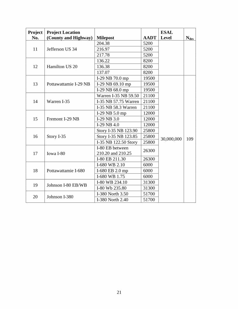
Introduction and Overview ................................................................................................18 Project Selection ................................................................................................................20 Evaluation of Existing Pavement Conditions ....................................................................23
Determination of Field Densities .......................................................................................26 Evaluation of the Gyratory Slope and PCCE .....................................................................28
Determination of Optimum Asphalt Content using Laboratory Compacted Mixes ..........29
CHAPTER 4: RESULTS AND ANALYSES ...............................................................................35
Pavement Performance Evaluation using PMIS and LTPP ...............................................35 Theoretical Maximum Specific Gravity QC/QA versus AASHTO T 209 ........................41 Change in Air Voids Post-Construction ............................................................................43 Air Voids at Construction and 4 Years Post-Construction ................................................46
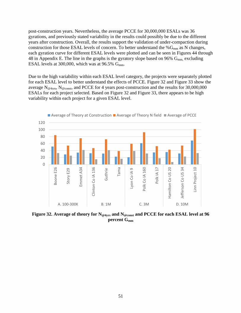
Air Voids at Construction and Post-Construction for 30,000,000 ESALs ........................47 Gyratory Compaction Slope and PCCE .............................................................................49 Optimum Binder Content Selection ...................................................................................54
Volumetric Characteristics of Mixtures .............................................................................55
CHAPTER 5: CONCLUSIONS AND RECOMMENDATIONS .................................................64
APPENDIX A: QC/QA FIELD VOIDS DATA (300,000–10,000,000 ESALS) ..........................69
vi
APPENDIX B: QC/QA LABORATORY VOIDS DATA (300,000–10,000,000 ESALS) ..........71
APPENDIX C: DATA AIR VOID ANALYSES (300,000–10,000,000 ESALS) ........................77
APPENDIX D: DENSITY INFORMATION (30,000,000 ESALS) .............................................79
APPENDIX E: GYRATION CURVES FOR EACH ESAL LEVEL ...........................................83
vii
LIST OF FIGURES
Figure 1. Gradation curves used in typical Superpave mixes ..........................................................5 Figure 2. HMA compaction device with California kneading compactor (left), Marshall
hammer (center), and Superpave Gyratory Compactor (right) .......................................7
Figure 3. AFG2 Superpave Gyratory Compactor ............................................................................7 Figure 4. Locations of NCHRP Project 9-9(1) field studies ............................................................9 Figure 5. Illinois 3-2-2 locking point .............................................................................................11 Figure 6. Concept of Ndesign ............................................................................................................11 Figure 7. Field-mix/laboratory-compacted (FMLC) versus field-mixed/field-compacted
(FMFC) air voids after 3 years ......................................................................................13 Figure 8. Severe rutting in flexible pavement ................................................................................14 Figure 9. Fatigue cracking (left) and pothole caused by fatigue cracking (right) ..........................15
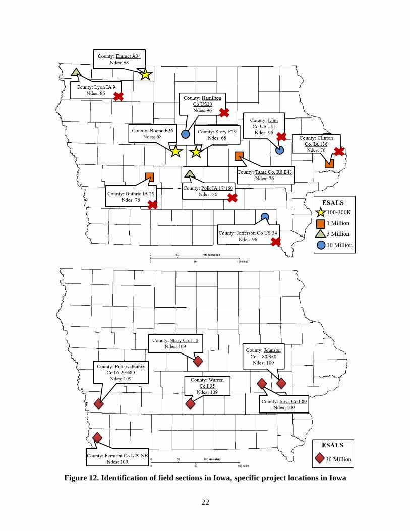
Figure 10. Block cracking, type of thermal cracking .....................................................................16 Figure 11. Flowchart of experimental plan for the study...............................................................19 Figure 12. Identification of field sections in Iowa, specific project locations in Iowa ..................22
Figure 13. Cumulative distribution of surface mixes.....................................................................23 Figure 14. Actual field core samples .............................................................................................26
Figure 15. Corelok method ............................................................................................................26 Figure 16. Water bath used in conventional method .....................................................................27 Figure 17. Metal bucket method (left) and flask method (right) ...................................................28
Figure 18. Conceptual representation of theoretical PCCE ...........................................................29 Figure 19. Aggregate gradation of different levels of traffic .........................................................32
Figure 20. At 1 million ESALs: (a) alligator or fatigue cracking, (b) transverse cracking,
(c) longitudinal cracking, and (d) rutting ......................................................................36
Figure 21. At 3 million ESALs: (a) alligator or fatigue cracking, (b) transverse cracking,
(c) longitudinal cracking, and (d) rutting ......................................................................37
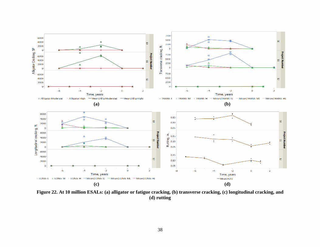
Figure 22. At 10 million ESALs: (a) alligator or fatigue cracking, (b) transverse cracking,
(c) longitudinal cracking, and (d) rutting ......................................................................38 Figure 23. IRI indication at each ESAL level ................................................................................39
Figure 24. Gmm estimated or QC/QA versus actual Gmm or Gmm tested in accordance with
AASHTO T 209 ............................................................................................................42
Figure 25. Calculated air voids with estimated Gmm from QC/QA data and air voids with
Gmm measured from the field core tested in accordance with AASHTO T 209 ...........42
Figure 26. Change in percent air voids per ESAL level at (a) 300,000, (b) 1,000,000, (c)
3,000,000, and (d) 10,000,000 ......................................................................................44 Figure 27. Change in percent air voids against ESALs (left) and distribution of the percent
change in air voids with varying ESAL levels (right)...................................................45
Figure 28. Average air voids at construction and 4 years post-construction .................................46 Figure 29. Percent air voids at construction versus air voids 4 years post-construction ...............47 Figure 30. Air void analysis for 30,000,000 ESALs......................................................................48
Figure 31. PCCE per ESAL level at 96 percent Gmm ....................................................................50 Figure 32. Average of theory for N@4yrs and N@const and PCCE for each ESAL level at 96
percent Gmm ...................................................................................................................51 Figure 33. Average of theory for N@4yrs and N@const and PCCE for 30,000,000 ESALs ...............52
viii
Figure 34. Distribution of percent of theoretical maximum density at construction with an
expected shifted distribution for air voids at 4 years post-construction........................53 Figure 35. Percent air void versus percent asphalt for all traffic levels .........................................55 Figure 36. Percent voids in asphalt mixture versus percent asphalt for all traffic levels ..............56
Figure 37. Percent voids filled with asphalt versus percent asphalt for all traffic levels ..............56 Figure 38. Percent of theoretical maximum density versus number of gyrations for high
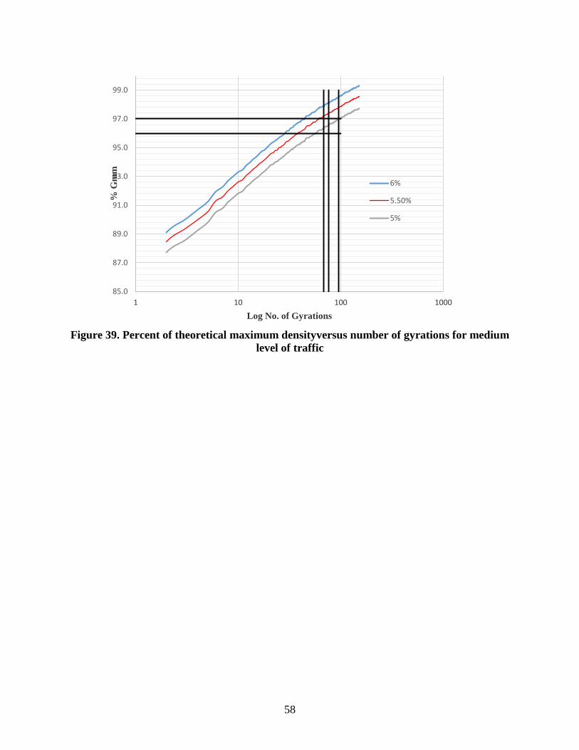
level of traffic ................................................................................................................57 Figure 39. Percent of theoretical maximum densityversus number of gyrations for medium
level of traffic ................................................................................................................58
Figure 40. Percent of theoretical maximum densityversus number of gyrations for low
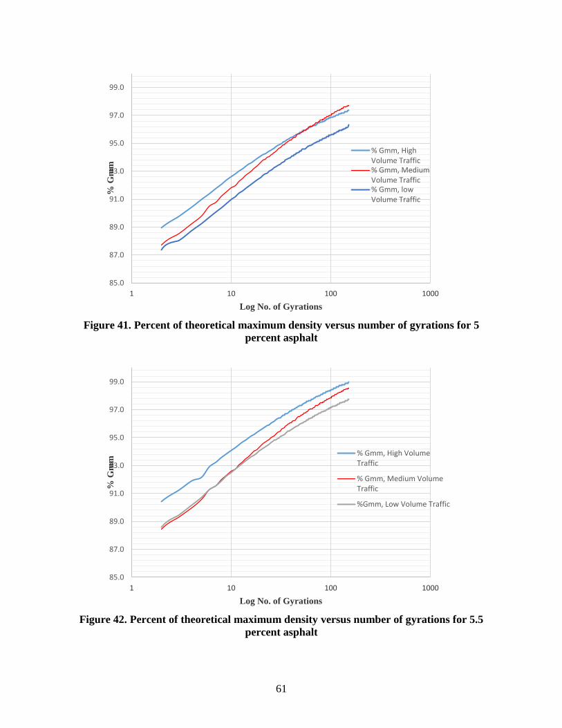
level of traffic ................................................................................................................59 Figure 41. Percent of theoretical maximum density versus number of gyrations for 5
Figure 44. Gyration curve for 300,000 ESALs ..............................................................................83 Figure 45. Gyratory curve for 1,000,000 ESALs...........................................................................84 Figure 46. Gyratory curve for 3,000,000 ESALs...........................................................................85
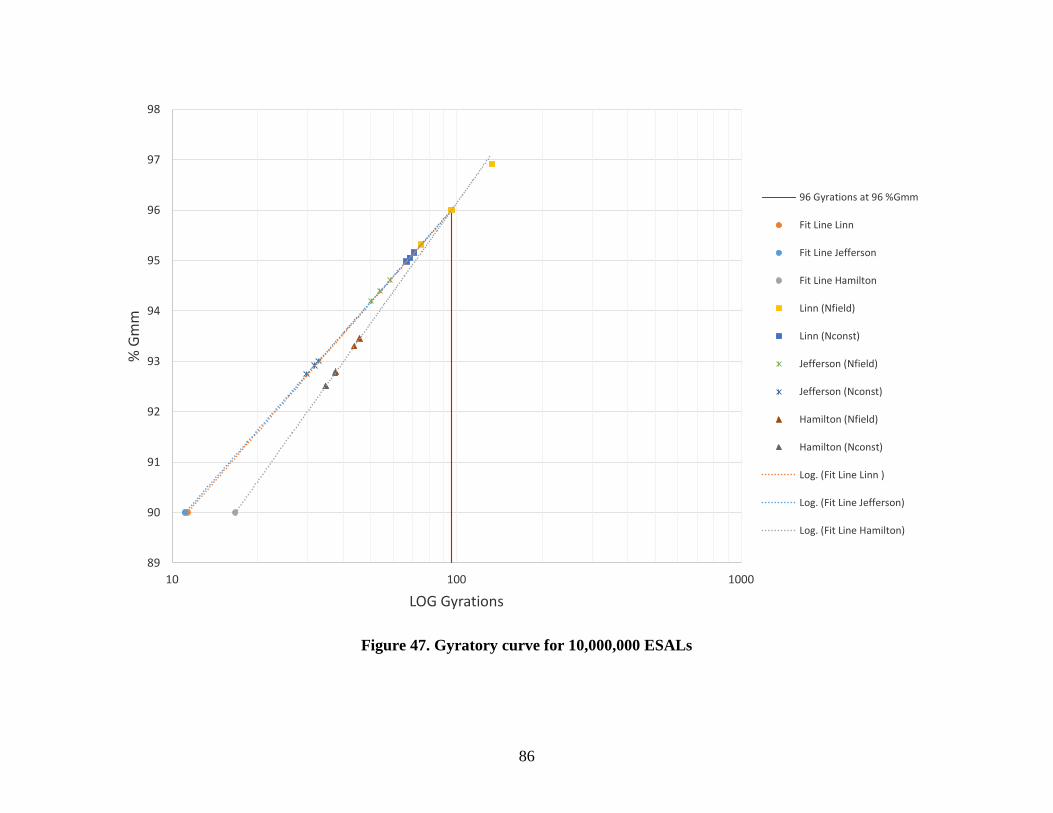
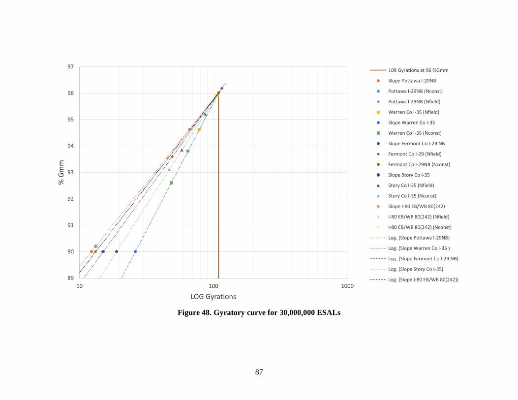
Figure 47. Gyratory curve for 10,000,000 ESALs.........................................................................86 Figure 48. Gyratory curve for 30,000,000 ESALs.........................................................................87
ix
LIST OF TABLES
Table 1. NCHRP compaction parameters ........................................................................................6 Table 2. NCHRP recommended Ndesign levels for a SGC DIA of 1.16° ± 2 ..................................12 Table 3. Project details ...................................................................................................................20
Table 4. Level of severity corresponding to type of distress .........................................................24 Table 5. Projects selected to evaluate pavement condition ............................................................25 Table 6. Aggregate gradation of low level of traffic .....................................................................30 Table 7. Aggregate gradation of medium level of traffic ..............................................................30 Table 8. Aggregate gradation of high level of traffic ....................................................................31
Table 9. Mix design properties of low-traffic level mix ................................................................33 Table 10. Mix design properties of medium-traffic level mix .......................................................33 Table 11. Mix design properties of high-traffic level mix .............................................................34
Table 12. Tabulation of average air voids for 30,000,000 ESALs ................................................49 Table 13. Compaction slope, theoretical N@field, and N@const .........................................................49 Table 14. Mixing and compaction temperatures............................................................................54
Table 15. Number of gyration for different levels of traffic ..........................................................54 Table 16. Summary of optimum asphalt content for all levels of traffic .......................................57
Table 17. Optimum asphalt contents for three types of mixtures under three different
design gyration numbers ...............................................................................................59 Table 18. Optimum asphalt contents for three types of mixtures under three different
design gyration numbers (4 percent air void for low level of traffic) ...........................60 Table 19. Percent air void for different levels of traffic, asphalt content, and number of
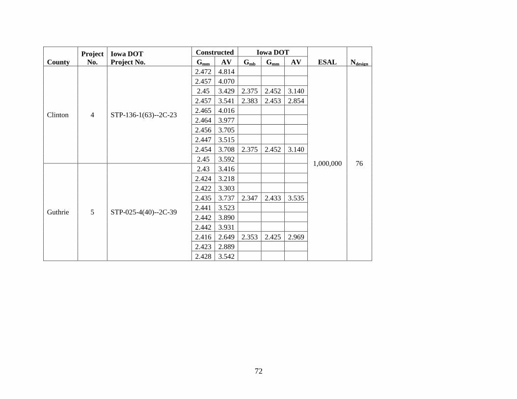
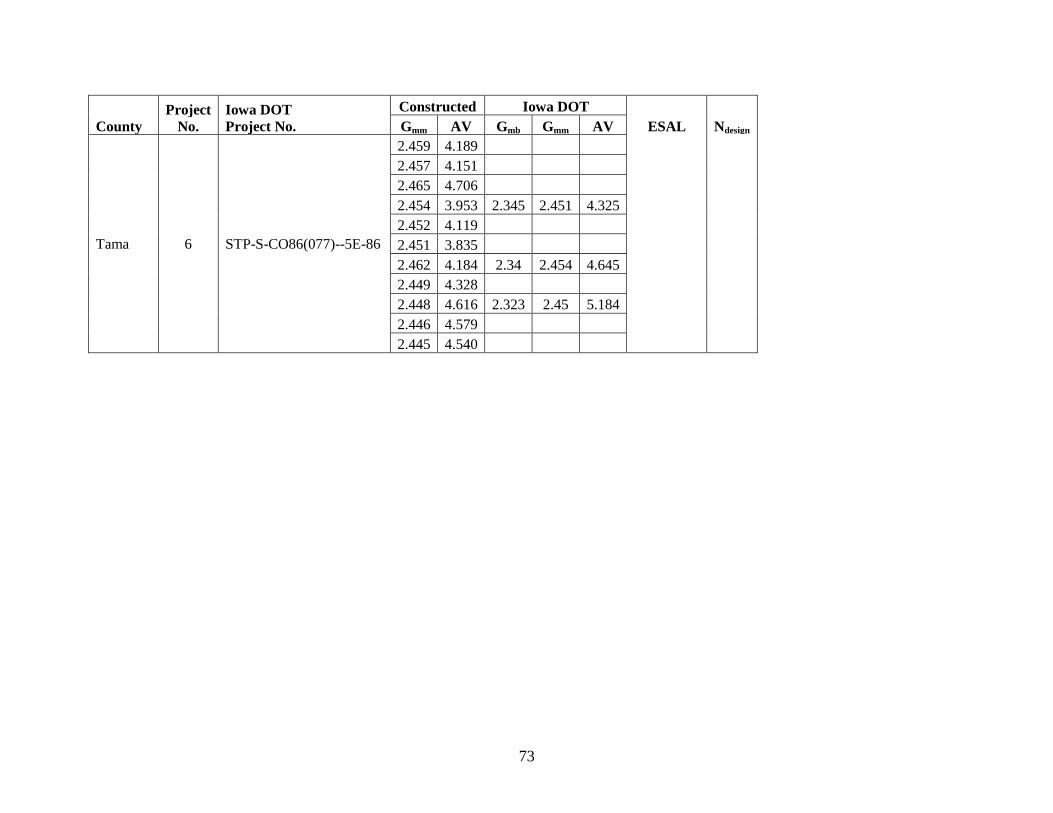
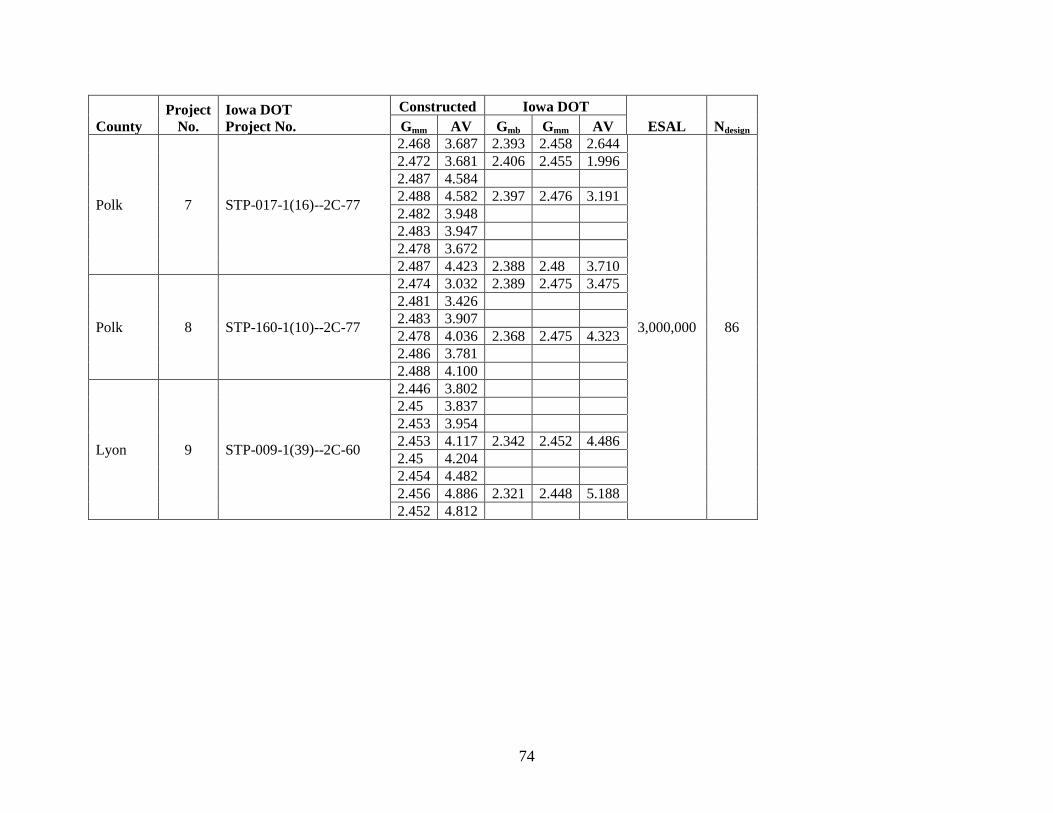
gyrations ........................................................................................................................63 Table 20. QC/QA field voids data for selected projects ................................................................69
Table 21. QC/QA laboratory voids data for selected projects .......................................................71 Table 22. Data for air void analyses ..............................................................................................77
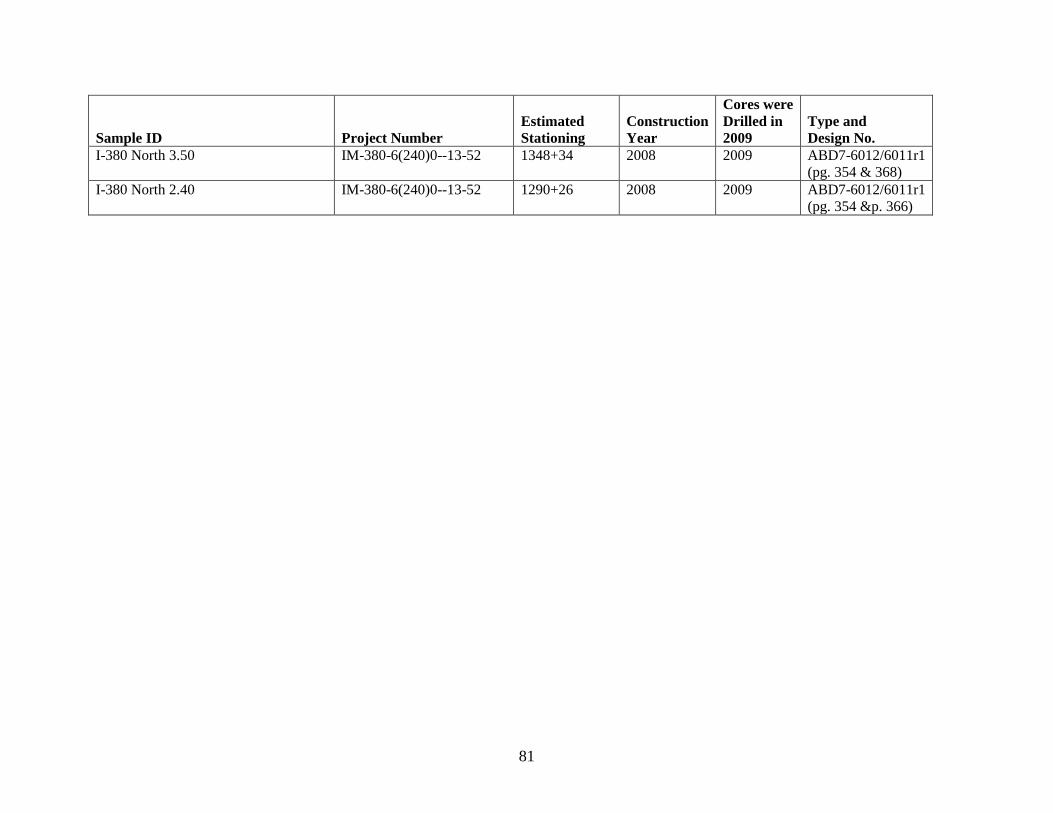
Table 23. Density information for 30,000,000 ESALs ..................................................................79 Table 24. Project information for 30,000,000 ESALs ...................................................................80
xi
ACKNOWLEDGMENTS
The authors would like to thank the Iowa Department of Transportation (DOT) and the Iowa
Highway Research Board (IHRB) for sponsoring this project and the Federal Highway
Administration (FHWA) for state planning and research funds that were used. We would also
like to thank Scott Schram with the Iowa DOT for his assistance during the duration of the
project. Special thanks go to the asphalt contractors for providing additional project information,
the asphalt materials research team/staff with the Iowa DOT, and district personnel for assisting
in field work, such as extracting cores required for this project.
xiii
EXECUTIVE SUMMARY
The design number of gyrations (Ndesign) introduced by the Strategic Highway Research Program
(SHRP) and used in the Superior Performing Asphalt Pavement (Superpave) mix design method
has been commonly used in flexible pavement design throughout the US since 1996. Ndesign, also
known as the compaction effort, is used to simulate field compaction during construction and has
been reported to produce air voids that are unable to reach ultimate pavement density within the
initial 2 to 3 years post-construction, potentially having an adverse impact on long-term
performance.
Other state transportation agencies have conducted similar validating the Ndesign for their specific
regions, which resulted in modifications of the gyration effort for the various traffic levels. This
study focused on the validation of Ndesign in Iowa.
Problem Statement and Objectives
The compaction effort is critical in asphalt mix design. Over-compaction during laboratory
design may lead to under-compaction in the field, reduced asphalt content, and can affect overall
durability. The objective of this study is to determine if the current mix design gyratory levels
are creating mixes that will attain target densification under traffic. The quality control and
quality assurance (QC/QA) information at construction were matched with field densities to
determine if traffic loading is adequately compacting the surface mix. Detailed objectives for the
project are outlined as follows:
1. Evaluate the ultimate in-place densities by performing volumetric testing for 300,000 to
30,000,000 equivalent single-axle loads (ESALs) for surface mixes in Iowa.
2. Determine the compatibility of mixes under the existing mix design procedures by
recalculating the gyratory slope from the QC/QA data.
3. Estimate and compare the post-construction compaction effort (PCCE) for each selected
project and determine the theoretical Ndesign at construction and post-construction.
4. Evaluate the optimum asphalt contents and aggregate structures due to different Ndesign values
adopted for the mixtures under three different traffic levels.
Experimental Plan
A total of 20 projects were selected within the six different Iowa Department of Transportation
(DOT) districts to evaluate the post-construction compaction effort and determine if 4% target
air voids were being achieved. Pavement sections constructed in 2011 for 300,000, 1,000,000,
3,000,000 and 10,000,000 ESALs, in addition to sections with varying construction and post-
construction years for 30,000,000 ESALs, were selected for the study.
xiv
All testing was done in accordance with the American Association of State Highway and
Transportation Officials (AASHTO) and ASTM International standards. Three sections per
ESAL level were selected, and pavement cores were removed by the Iowa DOT at three different
mileposts per project (excluding the 30,000,000 ESAL sections).
Pavement conditions were also evaluated based on available data using the Iowa DOT’s
Pavement Management Information System (PMIS) survey information and the Distress
Identification Manual for the Long-Term Pavement Performance Program (Miller and Bellinger
2003) to determine if the selected pavement sections displayed any anomalies during post-
construction.
The field densities, bulk specific gravity (Gmb), and theoretical maximum density (Gmm) of the
mixes were compared to the QC/QA data to determine the density during post-construction. The
field densities, in addition to the mix data, were also used to recalculate the gyratory compaction
slope.
With the determination of the compaction slope, the PCCE and the theoretical Ndesign at
construction and post-construction were determined for each mix. The theoretical Ndesign at
construction is the theoretical number of gyrations during construction, and, similarly, the
theoretical Ndesign post-construction is the theoretical amount of compaction induced by traffic
volume. Additionally, this study identifies the Ndesign values adopted for laboratory-
produced/laboratory-compacted mixes for low-, medium-, and high-traffic levels.
Conclusions and Recommendations
Based on the findings of the study, the following conclusions were found:
The current Ndesign compaction levels are higher than the targeted optimal value, creating
mixes that do not reach 4% air voids after traffic densification at 4 years post-construction.
These findings are consistent with other research studies conducted for other state
transportation agencies.
The majority of the mixes did not achieve 96% Gmm (or 4% air voids) at 1, 2, 4, and 12 years
post-construction (Note: Only ESAL levels below 30,000,000 were analyzed at 4 years post-
construction).
The overall pavement conditions displayed no signs of premature distresses on the pavements
studied. Pavement distresses showed that the overlay construction placed in 2011 provided
significant improvements in pavement performance.
The Gmm from the QC/QA data can be used to determine the density of the pavement since
the values of Gmm tested in the laboratory using field cores were close to the hotbox Gmm
values from the QC/QA data.
xv
Air void analysis showed that traffic volumes at the 300,000 and 3,000,000 ESAL levels
compacted better post-construction; whereas the 1,000,000, 10,000,000, and 30,000,000
ESAL levels were unable to densify to the target 4% in-situ air voids. The majority of the
sections at the two highest traffic volumes were unable to reach ultimate pavement density
with the current design gyrations.
Distribution of the %Gmm in years 2011, 2012, and 2013 indicate that at 4 years post-
construction there is a high probability that approximately 25% of the hot-mix asphalt
(HMA) mixtures will not attain ultimate pavement density.
In laboratory-produced/laboratory-compacted mixes for low-, medium-, and high-traffic
levels, the optimum asphalt content of the mixtures for a high-traffic level was lowest (at
4.8% for 4% air voids), followed by the medium-traffic level (at 5.68% for 4% air voids),
and the low-traffic level (at 5.8% for 3% air voids).
As Ndesign standards are reconsidered for the Iowa DOT, close attention to the design target
air voids, voids in the mineral aggregate (VMAs), and aggregate sources/types will need to
be addressed.
1
CHAPTER 1: INTRODUCTION
Background
The use of asphalt pavements, which cover about 94% of paved roads, has gradually increased
since the late 19th century(Brown et al. 2009). The mix design of asphalt pavements has
undergone continual evolution since initial development, relying heavily on empirical
knowledge. Past challenges with pavement distresses in asphalt concrete have shaped design
considerations in mix design and analysis. In the US, Superior Performing Asphalt Pavement
(Superpave) mix design is used in a majority of states.
One of the most important factors in design is the compaction effort of the asphalt mixture. The
compaction effort in the laboratory is known as the number of gyrations (N) and is denoted as
the initial number of gyrations (Ninitial), design number of gyrations (Ndesign), and maximum
number of gyrations (Nmax) in the Superpave mix design system. Ndesign is one of the most
significant design considerations/parameters in the laboratory and is selected based on the
corresponding equivalent single-axle load (ESAL) levels for the proposed pavement structure.
The initial Superpave values were selected based on studies that matched in-place densities to a
number of gyrations conducted by the Strategic Highway Research Program (SHRP) (Prowell
and Brown 2007).
Over time, many agencies and researchers have performed additional studies to validate gyratory
design levels (Harmelink and Aschenbrener 2002). Previous studies concluded that the Ndesign in
the Superpave mix design method is considerably higher than necessary, and, as a result, the
compaction effort conducted in the laboratory may not be reasonably attained in the field due to
differences in the compaction equipment, compaction procedure, and the difficultly of
compacting in the field.
During construction, the pavement is compacted in multiple lifts using rollers. Post-construction
compaction is expected to occur over time from traffic loading to achieve an ultimate pavement
density of 4% air voids within 2 to 3 years. However, studies have shown that if the Ndesign is too
high, the ultimate pavement density cannot be achieved within that timeframe. The primary
reason is the difficulty of compacting in the field, which consequently results in under-
compaction that can cause durability issues in the pavement. In addition, the aging of the asphalt
mixture is considerably affected by the initial air voids and temperature during production
(Brown et al. 2009).
Examination and modification, if needed, of the existing Ndesign table in Superpave mix design
would allow agencies to tailor the laboratory mix design process so 4% air voids can be achieved
from ultimate density.
While freight transportation begins to transition into more efficient and lower costs of moving
goods, the ability to store additional goods is more desired. As the evolution to modern highway
technology continues to grow rapidly, the industry will need to continuously improve and modify
2
standards/regulations to accommodate the changes in traffic volumes, environment, and the
automotive industry. Validation of the existing Ndesign table in the Superpave mix design will
allow agencies/researchers to better evaluate the field and laboratory pavement responses more
accurately. Ensuring adequate pavement density will reduce pavement distresses and improve
overall durability in the pavement.
Problem Statement
Ndesign has been used in the laboratory to compact specimens to a design ESAL level. The
existing Ndesign table in the Superpave mix design method has been reported to result in under-
compaction and thus lower asphalt content in the field. This may lead to difficulties in further
densifying the pavement, in addition to durability issues. Validating the asphalt mixes in Iowa
will provide better correlation between the target air voids and field air voids.
Objectives
The objective of this research was to validate current Ndesign levels for 300,000 to 30,000,000
ESAL level surface mix designs. Sections in Iowa from 2011 for ESAL levels below 30,000,000
were randomly selected at each ESAL level to evaluate 4 years post-construction. The
30,000,000 ESAL level sections were selected with varying post-construction years. Collection
of field cores and subsequent testing provided measurements of in-place densities 1, 2, 4, and 12
years post-construction.
The second objective was to determine the compactability of mixes under the current mix design
procedures by using the gyratory slope from quality control and quality assurance (QC/QA) data.
The post-construction compaction effort (PCCE) was evaluated as well as the optimum asphalt
content and aggregate structures with different Ndesign levels for laboratory-produced/laboratory-
compacted mixes for low, medium, and high traffic, and adjustments as needed were
recommended.
The third objective was to provide Ndesign recommendations for the laboratory designs used in
gyratory mix designs to the Iowa Department of Transportation (DOT), based on the findings of
this study.
Methods and Approach
The overall study focused primarily on the laboratory compaction effort or Ndesign. Testing was
done in accordance with the American Association of State Highway and Transportation
Officials (AASHTO) and ASTM International methods and procedures. The field cores used for
the study were provided by the Iowa DOT. The selected sections for the study were randomly
chosen throughout Iowa in the six Iowa DOT districts and varied in traffic volume. Pavement
condition surveys were also evaluated based on available data using the Pavement Management
Information System (PMIS) and the Long Term Pavement Performance Program (LTPP) manual
surveys.
3
Determination of air voids, both pre- and post-construction, were compared to QC/QA data and
analyzed accordingly. In addition, the gyratory slope and PCCE were evaluated for each project.
The research focused primarily on validating the effectiveness of the existing laboratory
compaction effort in Iowa; the theory or assumption of over-compaction in the laboratory
leading to under-compaction in the field has be examined in this study. Additionally, evaluation
of the optimum asphalt content from laboratory-produced/laboratory-compacted mixes for low,
medium, and high traffic were identified. The experimental plan is described in detail in
Chapter 3.
Significance of Work
The study has provided a better understanding of the overall effect of the existing Ndesign used in
Iowa. The outcome of the project will determine whether or not the Ndesign for Iowa should be
changed. The data collected will be used to provide a new Ndesign recommendation that will
influence asphalt mix designs and will be proposed for implementation upon laboratory
performance testing validation.
Organization
The following report is divided into five chapters. Chapter 1 provides the background to the
importance of the compaction effort in hot-mix asphalt (HMA), a problem statement, objectives,
methods and approach, and significance of work. Chapter 2 is the literature review, which
presents the previous studies conducted on the importance of lab and field compaction focused
on validating Ndesign. Chapter 3 provides details on the experimental plan and testing methods
used in this study. Chapter 4 presents the overall results and analyses. Chapter 5 summarizes the
conclusions and recommendations and provides ideas for future research in regards to identifying
an optimum Ndesign for Iowa and validating the performance of recommendations.
4
CHAPTER 2: LITERATURE REVIEW
History of Asphalt Mix Design
Early asphalt mixtures were primarily based on empirical design analysis (i.e., selecting
optimum asphalt content). Industries and agencies relied heavily on precedent experience to
evaluate and determine the appropriate mix type for selected sections at different locations with
varying temperatures. A good or bad mix would be differentiated based on the pavement
performance of the existing pavement structure, and the mechanics of the asphalt material was
not taken into consideration.
The use of HMA concrete significantly increased throughout the years, and the need for
standardized testing was essential to the design process (Christensen and Bonaquist 2005). Over
time, the use of empirical design was insufficient due to factors/variables varying significantly
with time. In the 1920s, the most popular early asphalt mix design method was the Hubbard-
Field mix design (Brown et al. 2009). The Hubbard-Field method later influenced the Marshall
and Hveem methods from the 1940s through the 1960s. In 1987, the Strategic Highway Research
Program (SHRP) began developing the Superpave mix design system, and, by 2008, most states,
including Iowa, adopted this mix design method (Prowell and Brown 2007).
The importance of simulating field compaction in the laboratory became one of the primary
concerns for the industry during the early implementation of mix design methods. Hveem
developed the Hveem mix design method in the mid-1920s for the California DOT (Caltrans, as
it’s known today), and the method was primarily used by western states (Brown et al. 2009). The
method was developed to improve pavement performance with the use of “oil mix” (a
combination of asphalt oil and aggregate) for low-traffic volume highways in California (Brown
et al. 2009). Hveem concluded that fine mixes required higher optimum asphalt content due to
their larger surface area as well as the appropriate amount of asphalt content from the particle
size distribution or gradation (Prowell and Brown 2007). The gradation in HMA is one of the
most effective means in determining the effectiveness of the performance of aggregate materials
as a pavement structure. Gradation is determined by passing aggregate materials through a series
of stacked sieves, which is known as sieve analysis (Brown et al. 2009). Figure 1 shows an
example of gradation curves used in HMA design.
5
Figure 1. Gradation curves used in typical Superpave mixes
Previous studies show that using more asphalt content on the aggregate particle thickens the film
and improves pavement durability (Hmoud 2011). The strength (or stability) of the mix was
tested using the Hveem stabilometer, and the kneading compaction was used to simulate field
compaction in the laboratory.
Because other states were unable to use the Hveem mix design method, in the late 1930s, the
Marshall method, introduced by Bruce Marshall, was implemented. The Marshall method
focused widely on the compaction effort of HMA and emphasized greatly on air voids.
In the early 1990s, with the limitations of the early mix design methods, SHRP developed the
Superpave mix design method (Brown et al. 2009). The Superpave mix design method primarily
focused on limiting/controlling detrimental pavement distresses. In order to do so, the mix design
takes into account the changes in environmental conditions, traffic load, and axle configurations.
Additionally, Superpave evaluates the asphalt binder, aggregate properties/characteristics,
mixture analysis, and the material and volumetric properties (of compacted samples) in the
HMA. These volumetrics were primarily used to determine the optimum asphalt content in the
mixture. The compaction device used to compact laboratory specimens is known as the
Superpave gyratory compactor (SGC), a compaction device similar to the original Texas
gyratory. The gyrations were heavily dependent on the traffic levels and were generally
expressed as 18,000 lbs ESAL. SHRP initially compacted samples at an angle of 1.0° but later
changed the internal angle of gyration to 1.16° (external angle 1.25°), with a constant vertical
6
pressure of 600 kilopascal (kPa) (Prowell and Brown 2007). Based on the National Cooperative
Highway Research Program (NCHRP) Project 9-9(1), Refinement of the Superpave Gyratory
Compaction Procedure, different levels of compaction effort were recommended for Superpave
and were denoted as Ninitial, Ndesign, and Nmax, as shown in Table 1 (Prowell and Brown 2007).
Table 1. NCHRP compaction parameters
Design ESALs
(millions)
Compaction Parameter
Ninitial Ndesign Nmaximum
< 0.3 6 50 75
0.3 to < 3 7 75 115
3 to < 30 8 100 160
> 30 9 125 205
Source: FHWA 2001
Because Superpave was designed only to test for asphalt binder and volumetric properties of a
mixture, agencies were hesitant to rely only on this, and as a result many researchers began using
supplemental tests such as the Hamburg Wheel-Tracking Device and the Asphalt Pavement
Analyzer (Brown et al. 2009). Inconsistent results were also observed between the density of
samples compacted at Ndesign and the density backcalculated from the Nmax. As a result, the
original Ndesign table was consolidated by creating an experimental matrix with 4 aggregate
sources, 2 gradations, and 6 Ndesign levels (40, 68, 93, 113, 139, and 172). As Ndesign was
increased, the optimum asphalt content, voids in the mineral aggregate (VMA), and voids filled
with asphalt (VFA) decreased with coarse-graded mixes being more sensitive than fine-graded
mixes.
Comparison of the Mix Design Methods
While the Hveem method is excellent in simulating field densities, this method is only developed
primarily for the western part of the US and is generally not recommended for use outside of that
region. In addition, the kneading compaction device is expensive and not portable and thus not
widely implemented. Alternatively, the Marshall mix design method uses an inexpensive and
simple compaction device. Both methods focused on the voids, strength, and durability of the
mix (NAPA 2015). Today, the Superpave mix design method is the most widely used method in
hot-mix asphalt design and analysis. In terms of compaction methods, the primary difference
between Superpave and the Marshall and Hveem methods is the ability of the SGC device to
monitor the change in height during the compaction process. The use of the gyratory compactor
lowered the VMA and optimum asphalt contents compared to the Marshall system. See Figure 2
and Figure 3for compaction devices.
7
FHWA (left and center) and ISU (right)
Figure 2. HMA compaction device with California kneading compactor (left), Marshall
hammer (center), and Superpave Gyratory Compactor (right)