171

!"#$"%&'!()*%+*,%*#-. !"*-$/(&(/("012333333 4!(-'5(/"*)(%))(//6"*(". 777777777777777786"*("9//*$-%"(:;%)+ /!("<*/#".=>("-%+/!("<*/#"8/:.?@(/*/*+(.A"(*/8=A?:.B( C#"/. D%$(/.7777777E(-)+#/"(.7777%<%-$("077777733 F%(' (%" ;"#-!%$(G#"&%/("@(/*/;%)+ #G)*(-)(%-?()@-#+#$ F()*/*#-&%(H @(F(%-4)#H("I2@122J
KLLMNOPQRQSNTOUOVWXYZP[TQZT\M]MQZ_QSNTOUOVW abcZP_QK\[TdeZffQgZU[\Z_[OTOLNQZ__PZTMLQPSOQLL[S[QT_Mhi[TVUQj[jQMk[_N\[LLQPQT_M]PLZSQ_PQZ_fQT_MZT\NQZ_Q\\QSlQUQfQT_mnoOUZPpO\Qqk[T_QP[rZ_[OTqsPS_[SqsT_ZPS_[SqjOUZPkZ_QPMqNQZ_UOMMqNQZ__PZTMLQPqNQZ__PZTMLQPSOQLL[S[QT_qSOTeQS_[eQNQZ__PZTMLQPqNQZ__PZTMLQPSOPPQUZ_[OTM `amtuvnavwnaKeQRO[ZMx]\fQM_Z\K\\cyPTzyUUZT\qxYpYZP[_[fQsi

M.Sc. ThesisMaster of Science in Engineering
Validation of heat transfer coefficientsSingle pipes with different surface treatments and heateddeck element
Bjarte Odin Kvamme
University of Stavanger2016

Department of Mechanical and Structural Engineering and Materials ScienceFaculty of Science and TechnologyUniversity of Stavanger
P.O. Box 8600 ForusN-4036 Stavanger, NorwayPhone +47 5183 [email protected]

SummaryThis master thesis has been written at the suggestion of GMC Maritime AS in agreement with theUniversity of Stavanger.
The interest in the polar regions is increasing, and further research is required to evaluate theadequacy of the equipment and appliances used on vessels traversing in polar waters. The decrease inice extent in the Arctic has renewed the interest in the Northern Sea Route. Oil and gas explorationhas moved further north during the past decades, and tourism in the polar regions is becoming morepopular. The introduction of the Polar Code by the International Maritime Organization attempts tomitigate some of the risks the vessels in Polar waters are exposed to.
This thesis investigates the adequacy of different theoretical methods of calculating the heat lossfrom cylinders and deck elements when exposed to a cross-wind scenario. Experiments were performedat GMC Maritime AS’s climate laboratory on Buøy, Stavanger. The experiments were performed on25 mm and 50 mm pipes with different surfaces, and on a deck element provided by GMC MaritimeAS. Theoretical calculations are performed and compared with heat transfer coefficients calculated fromexperimental data. Measurements in real-life conditions were recorded aboard the KV Svalbard duringa research project, SARex conducted off North Spitzbergen, April 2016. Statistics from this exerciseare presented. Findings are compared with requirements in the Polar Code and industry recommendedpractices from DNV GL.
Correlations for convective heat transfer over cylinders are evaluated and compared. Based on thefindings, the best correlation for use by the industry is selected and discussed. The arguments forselection were: Ease of use, Range of validity and Accuracy.
The correlation that was found to be best suited for single pipe configurations is the Churchill-Bernstein correlation. The deviation from the theoretical calculations to the experimental data for thiscorrelation was found to be in the range of 0.40 % to 1.61 % for a 50 mm insulated pipe and -3.86 %to -2.79 % for a 25 mm insulated pipe, depending on wind speed.
For deck elements only one correlation for the average heat transfer coefficient for a flat plate isfound in literature. This correlation is presented and used for theoretical calculations. The deviationsfrom theoretical to experimental values was significant, and more work is required to verify the accuracyof the correlation for flat plates.
The estimated time to freeze for water in a pipe is calculated for a range of diameters with varyingthicknesses of insulation at different wind speeds. Code for calculating the time to freeze is provided forfurther use by the reader. It is noted that to ensure the operation of pipe nozzles for fire extinguishingsystems, these must also have heat tracing, but this topic is not discussed further in this thesis.
Key elements for an optimal design of deck elements are suggested. Experiences from testing in thelaboratory and in the field are presented and discussed.
Keywords: Polar Code, winterization, Arctic, Antarctic, polar waters, heat loss, heat transfer, heattransfer coefficient, convective heat transfer, heat transfer correlations

ii

PrefaceThis thesis is dedicated to my unborn son. You haven’t arrived in this world yet, but your presence isalready noticeable and you have been the best inspiration and motivation one could imagine.
This master thesis was prepared at the Department of Mechanical and Structural Engineering andMaterials Science at the University of Stavanger in fulfilment of the requirements for acquiring a mastersdegree in Offshore Technology - Marine and Subsea technology.
The two years I have spent studying for my masters degree have been extremely fulfilling andinteresting. The courses I have taken have given me great insight into the challenges faced by theindustry, and methods that can be used to solve them.
During my studies, my interest in Arctic challenges has increased tremendously. I have takencourses at The University Centre of Svalbard in Arctic Offshore Engineering, and Arctic Operationsand Project Management at the University of Stavanger. These courses have given me invaluable insightin the working conditions and challenges revolving around operations in the Arctic. This interest wassparked and kept alive by Professor Ove Tobias Gudmestad, whom I am very grateful to have joinedacquaintance with. His interest and guidance has allowed me to write a conference paper which willbe presented at OMAE 2016 about weather windows offshore Norway. He also made it possible forme to participate in the SARex research project off North Spitzbergen. SARex was yet another veryinteresting and rewarding experience. It provided me with great insight on the challenges faced by theindustry with regards to the winterization design of equipment used in polar conditions.
Hopefully I will be able to continue my research into challenges in the Arctic, particularly relatedto the new requirements in the Polar Code. I have definitely got the taste of researching and hope tocontinue this work to a PhD level in the years to come.
All things considered, my six years at the University of Stavanger have been a great experience. Imet my partner, Oda Græsdal here and I have formed many acquaintances and friendships that willlast for the remainder of the foreseeable future.
That being said, graduates this year are facing difficult market conditions due to low oil prices.Very few positions related to marine engineering are posted, and even fewer are awarded to graduatestudents due to the abundance of experienced professionals available in the job market. I hope that myclassmates and myself are able to find work in the months to come, and that our paths will cross againin the future!
University of Stavanger, June 15, 2016
Bjarte Odin Kvamme

iv

AcknowledgementsThere have been numerous people involved in this thesis, especially for arranging all the practicalmatters surrounding the experimental tests. Jino Peechanatt has been my partner for the experimentalpart of this thesis, and our collaboration on this has gone without any problems, much thanks to hisexperience and knowledge.
My thanks go to GMC Maritime AS, both for allowing me to write this thesis for them, and for givingus access to their climate laboratory. Without their climate laboratory and support to SARex, thisthesis wouldn’t have been possible. I would like to thank Oddbjørn Hølland and Øystein Aasheim, whoworked for GMC Maritime AS during the majority of the work on this thesis, and Knut Espen Solbergwho is performing a PhD for GMC Maritime AS in conjunction with the University of Stavanger. All ofthem have proven invaluable for determining the scope of work, designing and procuring the equipmentneeded, and not least assisting when we were performing the testing in their facilities.
From the University of Stavanger, I would like to thank my supervisor, Professor Ove Tobias Gudmes-tad for his assistance in all aspects of writing this thesis. His assistance has been far more than whatcould have been expected. I would also like to thank Yaaseen Amith for his assistance with designingand constructing the testing jig. He also provided access to the 3D printing laboratory at the University,which allowed us to get perfect end caps for supporting the heating elements in the pipes. RomualdBernacki from the Department of Electrical Engineering and Computer Science has been of huge helpwhen designing the electrical circuits, teaching us how to solder, and provide wires, cables and other con-sumables. A huge thanks goes out to Tor Gulliksen and Jan Magne Nygård at the university workshopwho has provided assistance, consumables and directions in how to use the heavy machinery needed toprepare the components for the testing jig.
I would also like to give my thanks to Patrik Seldal Bakke, who has been a great resource in my questto learn how to program the Arduino, especially in debugging the problems I had with the real-timemonitoring of the data logger.
Least, but not least, I would like to express my utmost gratitude to my partner, Oda Græsdal, whothrough her excellent support for me, has allowed me to put in all the hours required to write thisthesis, not to mention all the time spent at the climate laboratory and during the field experiments.

vi

NomenclatureSymbol DescriptionA = Area, m2
d/D = Diameter, mg = Gravitational acceleration, m/s2
GMC = GMC Maritime ASh = Convective heat transfer coefficient, W/m2 · KI = Electrical current, Ak = Thermal conductivity, W/m · KK = Degrees Kelvin, unit of measurementm = Mass, kgNuD = Nusselt number, dimensionlessp = Pressure, N/m2
Pr = Prandtl number, dimensionlessq = Heat transfer rate, Wq′ = Heat transfer rate per unit length, W/mq′′ = Heat transfer rate per unit area, W/m2
r/R = Radius, mri = Inner radius, mro = Outer radius, mRair = Specific gas constant of air, 0.287kJ/kg · KRe = Electrical resistance, ΩRt = Thermal resistance, W/KReD = Reynolds number, dimensionlessRex,c = Critical Reynolds number, 5 × 10⁵
Tf = Film temperature, KTi = Internal temperature, KT∞ = Ambient / free-stream temperature, KTs = Surface temperature, Kt = Time, su∞ = Free-stream velocity, m/sU = Overall heat transfer coefficient, W/m2 · KV = Electrical potential / voltage, Vα = Thermal diffusivity, m2/sδ = Hydrodynamic boundary layer thickness, mδt = Thermal boundary layer thickness, mε = Emissivity, dimensionlessµ = Dynamic viscosity, N · s/m2
ν = Momentum diffusivity / kinematic viscosity, m2/sσ = Stefan-Boltzman’s constant, 5.6704 × 10⁻⁸ W/m2K4

ContentsSummary i
Preface iii
Acknowledgements v
Nomenclature vii
Contents viii
List of Figures xi
List of Tables xiii
1 Introduction 11.1 Scope of work . . . . . . . . . . . . . . . . . . . . . . . . . . . . . . . . . . . . . . . . . . 11.2 Thesis structure . . . . . . . . . . . . . . . . . . . . . . . . . . . . . . . . . . . . . . . . . 11.3 Schedule . . . . . . . . . . . . . . . . . . . . . . . . . . . . . . . . . . . . . . . . . . . . . 21.4 Background . . . . . . . . . . . . . . . . . . . . . . . . . . . . . . . . . . . . . . . . . . . 3
2 Theory 112.1 Fundamental concepts . . . . . . . . . . . . . . . . . . . . . . . . . . . . . . . . . . . . . 112.2 Heat transfer correlations . . . . . . . . . . . . . . . . . . . . . . . . . . . . . . . . . . . 182.3 Time to freeze . . . . . . . . . . . . . . . . . . . . . . . . . . . . . . . . . . . . . . . . . . 21
3 Calculations 273.1 Forced flow over a flat plate . . . . . . . . . . . . . . . . . . . . . . . . . . . . . . . . . . 273.2 Forced flow over an insulated pipe . . . . . . . . . . . . . . . . . . . . . . . . . . . . . . 313.3 Time to freeze . . . . . . . . . . . . . . . . . . . . . . . . . . . . . . . . . . . . . . . . . . 383.4 Calculating heat transfer coefficient from experimental data . . . . . . . . . . . . . . . . 42
4 Experiments 474.1 Equipment configuration . . . . . . . . . . . . . . . . . . . . . . . . . . . . . . . . . . . . 474.2 Laboratory experiments . . . . . . . . . . . . . . . . . . . . . . . . . . . . . . . . . . . . 524.3 Testing methodology . . . . . . . . . . . . . . . . . . . . . . . . . . . . . . . . . . . . . . 574.4 Field experiments . . . . . . . . . . . . . . . . . . . . . . . . . . . . . . . . . . . . . . . . 60
5 Results 635.1 Experiment 1 . . . . . . . . . . . . . . . . . . . . . . . . . . . . . . . . . . . . . . . . . . 645.2 Experiment 4 . . . . . . . . . . . . . . . . . . . . . . . . . . . . . . . . . . . . . . . . . . 665.3 Experiment 5 . . . . . . . . . . . . . . . . . . . . . . . . . . . . . . . . . . . . . . . . . . 685.4 Experiment 6 . . . . . . . . . . . . . . . . . . . . . . . . . . . . . . . . . . . . . . . . . . 705.5 Experiment 8 . . . . . . . . . . . . . . . . . . . . . . . . . . . . . . . . . . . . . . . . . . 725.6 Experiment 11 . . . . . . . . . . . . . . . . . . . . . . . . . . . . . . . . . . . . . . . . . 745.7 Deck element . . . . . . . . . . . . . . . . . . . . . . . . . . . . . . . . . . . . . . . . . . 76
Contents ix
5.8 Theoretical calculations . . . . . . . . . . . . . . . . . . . . . . . . . . . . . . . . . . . . 795.9 Comparison of theoretical calculations and laboratory experiments . . . . . . . . . . . . 885.10 Comparison of experiments . . . . . . . . . . . . . . . . . . . . . . . . . . . . . . . . . . 925.11 Statistics from field testing . . . . . . . . . . . . . . . . . . . . . . . . . . . . . . . . . . 955.12 Estimated time to freeze . . . . . . . . . . . . . . . . . . . . . . . . . . . . . . . . . . . . 98
6 Discussion 1016.1 Pipes . . . . . . . . . . . . . . . . . . . . . . . . . . . . . . . . . . . . . . . . . . . . . . . 1016.2 Deck element . . . . . . . . . . . . . . . . . . . . . . . . . . . . . . . . . . . . . . . . . . 105
7 Conclusions 1137.1 Future work . . . . . . . . . . . . . . . . . . . . . . . . . . . . . . . . . . . . . . . . . . . 114
Bibliography 115
A Arduino code used for temperature logger 117
B Code used for calculations 125
C Experiment logs 139
D Time to freeze tables 147
E Full experiment data logs 151

x

List of Figures1.1 10-year averages between 1979 and 2008 and yearly averages for 2007, 2012, and 2015 of the
daily (a) ice extent and (b) ice area in the Northern Hemisphere and a listing of the extentand area of the current, historical mean, minimum, and maximum values in km2 (Comiso,Parkinson, Markus, Cavalieri, & Gersten, 2015) . . . . . . . . . . . . . . . . . . . . . . . . . 4
1.2 Picture of the Goliat platform ©Eni Norge . . . . . . . . . . . . . . . . . . . . . . . . . . . . 51.3 Estimate of annual visitation for Arctic areas (Fay, Karlsdöttir, & Bitsch, 2010) . . . . . . . 61.4 Definition of boundaries in the Arctic (Ahlenius, 2007) . . . . . . . . . . . . . . . . . . . . . 91.5 Maximum extent of the Arctic waters (IMO, 2016) . . . . . . . . . . . . . . . . . . . . . . . 101.6 Maximum extent of the Antarctic waters (IMO, 2016) . . . . . . . . . . . . . . . . . . . . . 10
2.1 Conduction, convection and thermal radiation heat transfer (Incropera, DeWitt, Bergman, &Lavine, 2006) . . . . . . . . . . . . . . . . . . . . . . . . . . . . . . . . . . . . . . . . . . . . 11
2.2 Heat transfer through a composite material (Serth, 2007) . . . . . . . . . . . . . . . . . . . 142.3 Temperature distribution through a cylinder with composite walls (Incropera, DeWitt, Bergman,
& Lavine, 2006) . . . . . . . . . . . . . . . . . . . . . . . . . . . . . . . . . . . . . . . . . . . 152.4 Velocity boundary layer development over a flat plate (Incropera, DeWitt, Bergman, & Lavine,
2006) . . . . . . . . . . . . . . . . . . . . . . . . . . . . . . . . . . . . . . . . . . . . . . . . 18
4.1 Picture of the testing rig mounted on a pallet ©Bjarte Odin Kvamme . . . . . . . . . . . . . 474.2 Sketch of insulated pipe as tested . . . . . . . . . . . . . . . . . . . . . . . . . . . . . . . . . 484.3 Deck element positioned for testing . . . . . . . . . . . . . . . . . . . . . . . . . . . . . . . . 494.4 Breakout board used for connecting sensors ©Bjarte Odin Kvamme . . . . . . . . . . . . . . 504.5 Arduino based data logger, configured for testing ©Bjarte Odin Kvamme . . . . . . . . . . . 514.6 Screenshot of the climate laboratory control system . . . . . . . . . . . . . . . . . . . . . . 534.7 Picture of the test rig as installed in GMC’s climate laboratory ©Bjarte Odin Kvamme . . . 544.8 Overhead view of the test rig, with key components marked ©Bjarte Odin Kvamme . . . . . 544.9 Plot of wind speed / voltage from Tab. 4.6 . . . . . . . . . . . . . . . . . . . . . . . . . . . 554.10 Diagram of the wind nozzle with dimensions and measurement location . . . . . . . . . . . 564.11 Time series plot of Experiment 4 . . . . . . . . . . . . . . . . . . . . . . . . . . . . . . . . . 59
5.1 Sketch of the different zones used for calculating the overall heat transfer coefficient . . . . 635.2 Experiment 1: Overall heat transfer coefficient at different wind speeds . . . . . . . . . . . 645.3 Experiment 1: Overall heat transfer coefficient at different wind speeds, by section . . . . . 645.4 Experiment 4: Overall heat transfer coefficient at different wind speeds . . . . . . . . . . . 665.5 Experiment 4: Overall heat transfer coefficient at different wind speeds, by section . . . . . 665.6 Experiment 5: Overall heat transfer coefficient at different wind speeds . . . . . . . . . . . 685.7 Experiment 5: Overall heat transfer coefficient at different wind speeds, by section . . . . . 685.8 Experiment 6: Overall heat transfer coefficient at different wind speeds . . . . . . . . . . . 705.9 Experiment 6: Overall heat transfer coefficient at different wind speeds, by section . . . . . 705.10 Experiment 8: Overall heat transfer coefficient at different wind speeds . . . . . . . . . . . 725.11 Experiment 8: Overall heat transfer coefficient at different wind speeds, by section . . . . . 725.12 Experiment 11: Overall heat transfer coefficient at different wind speeds . . . . . . . . . . . 745.13 Experiment 11: Overall heat transfer coefficient at different wind speeds, by section . . . . 74

xii List of Figures
5.14 Plot of overall heat transfer coefficient versus wind speed for the deck element . . . . . . . . 765.15 Plot of power consumption versus wind speed for the deck element . . . . . . . . . . . . . . 765.16 Experiment 1: Theoretical overall heat transfer coefficients at different wind speeds . . . . . 795.17 Experiment 1: Theoretical overall heat transfer coefficients at different wind speeds at Section 2 805.18 Experiment 8: Theoretical overall heat transfer coefficients at different wind speeds . . . . . 825.19 Experiment 8: Theoretical overall heat transfer coefficients at different wind speeds, by section 825.20 Experiment 11: Theoretical overall heat transfer coefficients at different wind speeds . . . . 845.21 Experiment 11: Theoretical overall heat transfer coefficients at different wind speeds, by section 845.22 Experiment 1, Section 2: Overall heat transfer coefficients, theoretical versus experimental
data . . . . . . . . . . . . . . . . . . . . . . . . . . . . . . . . . . . . . . . . . . . . . . . . . 885.23 Experiment 8, Section 2: Overall heat transfer coefficients, theoretical versus experimental
data . . . . . . . . . . . . . . . . . . . . . . . . . . . . . . . . . . . . . . . . . . . . . . . . . 895.24 Experiment 11, Section 2: Overall heat transfer coefficients, theoretical versus experimental
data . . . . . . . . . . . . . . . . . . . . . . . . . . . . . . . . . . . . . . . . . . . . . . . . . 895.25 Deck element testing: Overall heat transfer coefficients, theoretical versus experimental data 915.26 Deck element testing: Total power consumption, theoretical versus experimental data . . . 925.27 Comparison of Experiment 1, 4, 5, 6 and 11 . . . . . . . . . . . . . . . . . . . . . . . . . . . 935.28 Comparison of Experiment 1, 4, 5 and 6 . . . . . . . . . . . . . . . . . . . . . . . . . . . . . 935.29 Time series plot of overall heat transfer coefficient versus wind speed for the uninsulated pipe 955.30 Time series plot of overall heat transfer coefficient versus wind speed for the insulated pipe 955.31 Time series plot of temperatures versus wind speed for the uninsulated pipe . . . . . . . . . 965.32 Time series plot of temperatures versus wind speed for the for the insulated pipe . . . . . . 96
6.1 Pipe with ice glazing as tested ©Bjarte Odin Kvamme . . . . . . . . . . . . . . . . . . . . . 1026.2 Insulated pipe with glued quartz particles versus a normal, insulated pipe ©Bjarte Odin
Kvamme . . . . . . . . . . . . . . . . . . . . . . . . . . . . . . . . . . . . . . . . . . . . . . . 1036.3 Deck element inside pallet boxes to remove any wind from the evaporators. ©Bjarte Odin
Kvamme . . . . . . . . . . . . . . . . . . . . . . . . . . . . . . . . . . . . . . . . . . . . . . . 1086.4 Ice accumulation on fire extinguishing nozzle on KV Svalbard. Picture taken in April 2016,
west of Ny Ålesund. Ambient temperature was -12 C and no wind apart from the air flowcaused by the transit at 13 knots. ©Trond Spande . . . . . . . . . . . . . . . . . . . . . . . 109
6.5 Snow and ice accumulation on the helicopter deck on KV Svalbard. Picture taken in April2016, west of Ny Ålesund. Ambient temperature was -12 C and no wind apart from the airflow caused by the transit at 13 knots. ©Trond Spande . . . . . . . . . . . . . . . . . . . . . 110
6.6 Thermal image of the starboard side of the helicopter deck. Heat tracing is visible as theyellow lines in a grid. ©Trond Spande . . . . . . . . . . . . . . . . . . . . . . . . . . . . . . 111

List of Tables1.1 Tasks and time spent . . . . . . . . . . . . . . . . . . . . . . . . . . . . . . . . . . . . . . . . 2
2.1 Constants for use with Sutherland’s law (2.28) . . . . . . . . . . . . . . . . . . . . . . . . . 172.2 Constants originally proposed by Hilpert (1933) . . . . . . . . . . . . . . . . . . . . . . . . . 192.3 Updated constants for use with the Hilpert correlation (Çengel, 2006; Incropera, DeWitt,
Bergman, & Lavine, 2006; Moran, Shapiro, Munson, & DeWitt, 2003) . . . . . . . . . . . . 192.4 Reviewed values of C and m (Fand & Keswani, 1973) . . . . . . . . . . . . . . . . . . . . . 202.5 Reviewed values of C and m (Morgan, 1975) . . . . . . . . . . . . . . . . . . . . . . . . . . 202.6 Values of n for different Prandtl numbers (Žukauskas, 1972) . . . . . . . . . . . . . . . . . . 202.7 Suggested values of C and m (Žukauskas, 1972) . . . . . . . . . . . . . . . . . . . . . . . . . 20
3.1 Constants used in calculations for flat plate . . . . . . . . . . . . . . . . . . . . . . . . . . . 283.2 Constants used in calculations for insulated pipe . . . . . . . . . . . . . . . . . . . . . . . . 313.3 Comparison of example theoretical calculations . . . . . . . . . . . . . . . . . . . . . . . . . 383.4 Constants used in the calculation of required time to freeze . . . . . . . . . . . . . . . . . . 393.5 Constants used in the calculation of the heat transfer coefficient of a flat plate from experi-
mental data . . . . . . . . . . . . . . . . . . . . . . . . . . . . . . . . . . . . . . . . . . . . . 433.6 Constants used in the calculation of the heat transfer coefficient of a uninsulated pipe from
experimental data . . . . . . . . . . . . . . . . . . . . . . . . . . . . . . . . . . . . . . . . . 433.7 Constants used in the calculation of the heat transfer coefficient of a insulated pipe from
experimental data . . . . . . . . . . . . . . . . . . . . . . . . . . . . . . . . . . . . . . . . . 44
4.1 Resistances of heating elements . . . . . . . . . . . . . . . . . . . . . . . . . . . . . . . . . . 484.2 Key components of tested deck element as shown in Fig. 4.3 . . . . . . . . . . . . . . . . . 494.3 Description of key components on breakout board as shown in Fig. 4.4 . . . . . . . . . . . 504.4 Calibrated offset of temperature and humidity sensors . . . . . . . . . . . . . . . . . . . . . 524.5 Key components of testing rig . . . . . . . . . . . . . . . . . . . . . . . . . . . . . . . . . . . 524.6 Measured output voltages at different wind speeds . . . . . . . . . . . . . . . . . . . . . . . 534.7 Corrected wind speed measurements . . . . . . . . . . . . . . . . . . . . . . . . . . . . . . . 554.8 Experiments performed . . . . . . . . . . . . . . . . . . . . . . . . . . . . . . . . . . . . . . 57
5.1 Description of headers used in results . . . . . . . . . . . . . . . . . . . . . . . . . . . . . . 635.2 Temperatures and overall heat transfer coefficients, Experiment 1 . . . . . . . . . . . . . . . 655.3 Temperatures and overall heat transfer coefficients, Experiment 4 . . . . . . . . . . . . . . . 675.4 Temperatures and overall heat transfer coefficients, Experiment 5 . . . . . . . . . . . . . . . 695.5 Temperatures and overall heat transfer coefficients, Experiment 6 . . . . . . . . . . . . . . . 715.6 Temperatures and overall heat transfer coefficients, Experiment 8 . . . . . . . . . . . . . . . 735.7 Temperatures and overall heat transfer coefficients, Experiment 11 . . . . . . . . . . . . . . 755.8 Measurements from deck element at -15 C and -20 C . . . . . . . . . . . . . . . . . . . . . 775.9 Measurements from deck element at -30 C and -35 C . . . . . . . . . . . . . . . . . . . . . 785.10 Nusselt number, average and overall heat transfer coefficients, theoretical, based on Experi-
ment 1 . . . . . . . . . . . . . . . . . . . . . . . . . . . . . . . . . . . . . . . . . . . . . . . . 81

xiv List of Tables
5.11 Nusselt number, average and overall heat transfer coefficients, theoretical, based on Experi-ment 8 . . . . . . . . . . . . . . . . . . . . . . . . . . . . . . . . . . . . . . . . . . . . . . . . 83
5.12 Nusselt number, average and overall heat transfer coefficients, theoretical, based on Experi-ment 11 . . . . . . . . . . . . . . . . . . . . . . . . . . . . . . . . . . . . . . . . . . . . . . . 85
5.13 Description of headers used in deck element heat transfer calculations . . . . . . . . . . . . 865.14 Theoretical heat transfer calculations of deck element . . . . . . . . . . . . . . . . . . . . . 875.15 Summary of deviations between experimental and theoretical values for Experiment 1, 8 and
11 . . . . . . . . . . . . . . . . . . . . . . . . . . . . . . . . . . . . . . . . . . . . . . . . . . 885.16 Comparison of theoretical and experimental values for Experiment 1 and 8 at Section 2 of
the pipes . . . . . . . . . . . . . . . . . . . . . . . . . . . . . . . . . . . . . . . . . . . . . . 905.17 Comparison of theoretical and experimental values for Experiment 11 at Section 2 of the pipes 915.18 Comparison of theoretical and experimental values for deck element testing . . . . . . . . . 925.19 Comparison of Experiment 1, 4, 5, 6 . . . . . . . . . . . . . . . . . . . . . . . . . . . . . . . 945.20 Statistics from field testing, overall heat transfer coefficients and temperatures . . . . . . . 975.21 Time required to freeze 25 mm and 50 mm pipe . . . . . . . . . . . . . . . . . . . . . . . . . 985.22 Time required to freeze 25 mm and 50 mm pipe . . . . . . . . . . . . . . . . . . . . . . . . . 99
C.1 Experiment 1 - 1 x 50 mm pipe (O x x) . . . . . . . . . . . . . . . . . . . . . . . . . . . . . 139C.2 Experiment 2 - 2 x 50 mm pipe (O x O) . . . . . . . . . . . . . . . . . . . . . . . . . . . . . 139C.3 Experiment 3 - 3 x 50 mm pipe (O O O) . . . . . . . . . . . . . . . . . . . . . . . . . . . . 140C.4 Experiment 4 - 50 mm pipe with ice glazing . . . . . . . . . . . . . . . . . . . . . . . . . . . 140C.5 Experiment 5 - 50 mm pipe with ice coating . . . . . . . . . . . . . . . . . . . . . . . . . . . 141C.6 Experiment 6 - 50 mm pipe with roughened surface (0.7 - 1.2 mm particle size) . . . . . . . 141C.7 Experiment 7 - 1 x 25 mm + 1 x 50 mm (o x O) . . . . . . . . . . . . . . . . . . . . . . . . 142C.8 Experiment 8 - 1 x 25 mm pipe (o x x) . . . . . . . . . . . . . . . . . . . . . . . . . . . . . 142C.9 Experiment 9 - 2 x 25 mm pipe (o x o) . . . . . . . . . . . . . . . . . . . . . . . . . . . . . . 143C.10 Experiment 10 - 1 x 50 mm, 1 x 25 mm (O x o) . . . . . . . . . . . . . . . . . . . . . . . . . 143C.11 Experiment 11 - 1 x 50 mm pipe, no insulation (O x x) . . . . . . . . . . . . . . . . . . . . 144C.12 Experiment 12 - Deck element . . . . . . . . . . . . . . . . . . . . . . . . . . . . . . . . . . 145
D.1 Hours required to freeze 25, 50, 100, 500 and 1000 mm pipes with insulation thickness of 0,5, 10, 50 mm under 0.05 m/s wind speed . . . . . . . . . . . . . . . . . . . . . . . . . . . . 147
D.2 Hours required to freeze 25, 50, 100, 500 and 1000 mm pipes with insulation thickness of 0,5, 10, 50 mm under 5 m/s wind speed . . . . . . . . . . . . . . . . . . . . . . . . . . . . . . 148
D.3 Hours required to freeze 25, 50, 100, 500 and 1000 mm pipes with insulation thickness of 0,5, 10, 50 mm under 10 m/s wind speed . . . . . . . . . . . . . . . . . . . . . . . . . . . . . 149
D.4 Hours required to freeze 25, 50, 100, 500 and 1000 mm pipes with insulation thickness of 0,5, 10, 50 mm under 15 m/s wind speed . . . . . . . . . . . . . . . . . . . . . . . . . . . . . 150

CHAPTER 1Introduction
1.1 Scope of workThe following scope of work was agreed upon between GMC Maritime AS and the University of Sta-vanger.
1. Assess the relevant theoretical methods and industry standards used for describing the heat trans-fer from heated deck elements and for pipes exposed to a cross-flow wind arrangement. For pipes,insulation and heat transfer bridges (e.g. pipe supports) must be included in the methodology.
2. Based on the findings in Task 1, suggest the best method for use by the industry for describingthe heat transfer from pipes and decks, and document the argumentation behind. The argumentsbelow must be taking into consideration.
a) Ease of useb) Range of validityc) Accuracy
3. Develop a test methodology for testing the heat transfer from the pipes and heated deck elements,conforming to industrial usage scenarios (including ice cover), and perform experiments to validatethe findings in Task 1. Heated deck elements for testing shall be obtained from GMC. The testingrig for the heat transfer from pipes needs to be designed, procured and assembled.
4. Define the deviation between the theoretical and experimental approaches for each case.
5. Develop tables describing the required time to freeze for different diameters and different degreesof insulation based on the theoretical approach, with correctional factors (if required) from theexperimentation.
6. Based on findings from the theoretical and experimental approaches:
a) Define key elements to be considered for an optimal design of the deck elements.b) Recommend a design that fulfils industry requirements.
1.2 Thesis structureChapter 2 presents the relevant theory and the heat transfer correlations that will be addressed. Thiscovers Task 1 of the scope of work.
In Chapter 3 examples of the calculation for each correlation are presented, compared and discussed.This covers Task 2 of the scope of work.
Testing methodology was developed and equipment used for testing was designed and procured.The setup is presented in Chapter 4. Experimental testing was performed in GMC Maritime’s climatelaboratory. The results are presented in Chapter 5.1 to 5.7. Field testing was performed on the coastguard vessel KV Svalbard as part of the SARex research project on Svalbard. Statistics from the fieldexperiments are presented in Chapter 5.11. This covers Task 3 of the scope of work.
2 1 Introduction
Theoretical calculations at the same conditions were performed and are presented in Chapter 5.8.A comparison between the experimental values and the theoretical values are presented in Chapter 5.9.This covers Task 4 of the scope of work.
Tables with estimated the required time for water to freeze for different pipe diameters and insulationthicknesses in different conditions is presented in Chapter 5.12. Both the uncorrected values and thevalues with the deviation found in Chapter 5.9 are presented. This covers Task 5 of the scope of work.
Key elements for optimal deck element design and a recommended design are presented in Chapter6.2.1. This covers Task 6 of the scope of work.
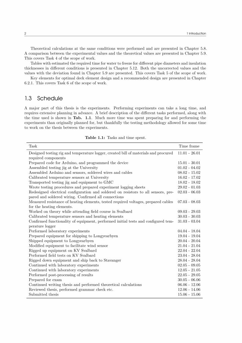
1.3 ScheduleA major part of this thesis is the experiments. Performing experiments can take a long time, andrequires extensive planning in advance. A brief description of the different tasks performed, along withthe time used is shown in Tab. 1.1. Much more time was spent preparing for and performing theexperiments than originally planned for, but thankfully the testing methodology allowed for some timeto work on the thesis between the experiments.
Table 1.1: Tasks and time spent.
Task Time frameDesigned testing rig and temperature logger, created bill of materials and procuredrequired components
11.01 - 26.01
Prepared code for Arduino, and programmed the device 15.01 - 30.01Assembled testing jig at the University 01.02 - 04.02Assembled Arduino and sensors, soldered wires and cables 08.02 - 15.02Calibrated temperature sensors at University 16.02 - 17.02Transported testing jig and equipment to GMC 18.02 - 18.02Wrote testing procedures and prepared experiment logging sheets 29.02 - 01.03Redesigned electrical configuration and soldered on resistors to all sensors, pre-pared and soldered wiring. Confirmed all connections
02.03 - 06.03
Measured resistance of heating elements, tested required voltages, prepared cablesfor the heating elements.
07.03 - 08.03
Worked on theory while attending field course in Svalbard 09.03 - 29.03Calibrated temperature sensors and heating elements 30.03 - 30.03Confirmed functionality of equipment, performed initial tests and configured tem-perature logger
31.03 - 03.04
Performed laboratory experiments 04.04 - 18.04Prepared equipment for shipping to Longyearbyen 19.04 - 19.04Shipped equipment to Longyearbyen 20.04 - 20.04Modified equipment to facilitate wind sensor 21.04 - 21.04Rigged up equipment on KV Svalbard 22.04 - 22.04Performed field tests on KV Svalbard 23.04 - 28.04Rigged down equipment and ship back to Stavanger 28.04 - 28.04Continued with laboratory experiments 02.05 - 09.05Continued with laboratory experiments 12.05 - 21.05Performed post-processing of results 22.05 - 29.05Prepared for exam 30.05 - 06.06Continued writing thesis and performed theoretical calculations 06.06 - 12.06Reviewed thesis, performed grammar check etc. 12.06 - 14.06Submitted thesis 15.06 - 15.06

1.4 Background 3
1.4 BackgroundThe activity level in the Polar regions is increasing and is expected to continue to increase over the nextyears. Oil and gas production, shipping, fishing and military activity are all areas that are expectedto increase over the coming years. The Arctic has multiple commonly used definitions, depending onwhich aspects you are interested in. These definitions are presented on a map in Fig. 1.4.
1.4.1 ShippingThe ice extent in the Arctic has decreased in the last decades, as shown in Fig. 1.1, particularlyduring the summer season. The decrease in the ice extent makes the Northern Sea Route (NSR) a moreviable option for shipping. The Northern Sea Route is a shipping lane between the Atlantic Oceanand the Pacific Ocean, which goes along the coastline of Siberia and the Far East. A route suggestedby Dubey (2012) is: Barents Sea - Kara Sea - Laptev Sea - East Siberian Sea - Chukchi Sea. Dubey(2012) estimates a saving of 17.5 days and 493 million tons of fuel when going through the NorthernSea Route, and emission savings of 50 tons of NOx, 1557 tons of CO2 and 35 tons of SOx. Costs foradditional insurance and ice breaker assistance needs to be taken into consideration, but these costswill likely decrease over time if the Northern Sea Route becomes a more common option.
1.4.2 Oil and gasWhile current oil prices do not easily allow for a significant development of the oil and gas resourcesin the Arctic, demand for oil and gas in 2035 is expected to increase by 18 % and 44 % respectively(Zolotukhin, 2014). 60 % of the planned oil and gas production in 2035 is estimated to come from fieldsthat have not yet been discovered (Zolotukhin, 2014). In 2000, The United States Geological Survey(USGS) estimated that a total of 25 % of the undiscovered oil and gas reserves are located in the Arctic.Considering that the Arctic only composes 6 % of the world’s area, this is a significant amount. In May2008, the USGS completed an assessment of the conventional, undiscovered oil and gas resources northof the Arctic Circle. This assessment was performed using a geology-based probabilistic methodology.In the assessment, it is estimated that a total of 90 billion barrels of oil, 1669 trillion cubic feet ofnatural gas, and 44 billion barrels of natural gas liquids could be present in Arctic regions, of which 84% is expected to be located in offshore areas (Bird et al., 2008).
Despite the increased cost of oil and gas exploration in remote, Arctic areas, it is expected that therise in demand will cause the exploration and production for oil and gas in the Arctic to increase. Thiswill result in more seismic survey vessels and exploration drilling vessels in the Arctic, and eventuallyoil and gas producing vessels.
Exploration and production vessels and platforms are highly dependent on the piping facilities, andthe ability to maintain flow assurance is crucial. If the winterization of pipes is not done properly, thiscould lead to massive costs due to production shut-down or even worse, accidents. A temperature dropbetween the different areas of the production facilities will change the thermodynamic properties of thefluids, and can in a best case scenario cause the processing of the crude oil to become inefficient. EniNorge has just finished installation and commissioning of the Goliat platform in the Barents Sea. TheGoliat platform is a cylindrical FPSO, where the production facilitates are partially enclosed to protectequipment and crew from the wind and weather in the Barents Sea. A picture of the Goliat platformis found in Fig. 1.2. Production facilities cannot be fully enclosed, as ventilation is still required incase of an unexpected release of gases. The use of fans to provide ventilation is likely to be sufficientunder normal conditions, but cannot be relied upon for emergency scenarios as loss of power might takeoccur. The compact design of the cylindrical FPSO allows for relatively easy wind protection. Otherhull designs such as ship-shaped FPSOs could be more difficult to protect from wind in a cost-effectivemanner.

4 1 Introduction
Figure 1.1: 10-year averages between 1979 and 2008 and yearly averages for 2007, 2012, and 2015 ofthe daily (a) ice extent and (b) ice area in the Northern Hemisphere and a listing of theextent and area of the current, historical mean, minimum, and maximum values in km2
(Comiso, Parkinson, Markus, Cavalieri, & Gersten, 2015).
1.4.3 TourismTourism and travel to polar regions is getting more popular, and the number of shipborne tourists inAntarctica increased from around 10 000 in 1992, to over 30 000 in 2007 (Ahlenius, 2007). Fig. 1.3shows that the number of tourists in Arctic areas is even higher, and is expected to continue to increaseover the coming years.
Accidents in polar waters are not unheard of. The vessel Maxim Gorkiy struck an iceberg in theGreenland Sea outside of Svalbard in 1989 (Lohr, 1989), leading to the evacuation of almost 1000passengers. The passengers were rescued by the Norwegian Coast Guard vessel KV Senja, whicharrived around four hours after the first distress call was made by the Maxim Gorkiy. Other major

1.4 Background 5
Figure 1.2: Picture of the Goliat platform ©Eni Norge.
accidents include the vessel MV Explorer with 154 persons aboard, which sank outside of Antarcticain 2007. The MV Explorer was the first tourist ship ever to sink off Antarctica (Bowermaster, 2007).The vessel MS National Geographic Endeavour arrived just four hours after the distress call was made,and observed that some passengers were already starting to show signs of minor hypothermia after fourhours in the lifeboats (Bowermaster, 2007). Common for both accidents are that under slightly differentcircumstances, they could have ended very badly for the passengers and crew members aboard. Majoraccidents in the Arctic and Antarctica are thankfully not frequent, mostly due to the limited numberof vessels travelling in these waters. Considering the increase in both the number of vessels, and thesize of the vessels, it becomes apparent that stricter regulations should be implemented to reduce therisks associated with the travel.
1.4.4 Polar CodeThe International Maritime Organization (IMO) has adopted the International Code for Ships Oper-ating in Polar Waters (Polar Code) and related amendments, and has made it mandatory under theInternational Convention of the Safety of Life at Sea (SOLAS). The Polar Code was adopted in Novem-ber 2014, and is expected to enter into force on 01.01.2017. It applies to ships operating in Arctic andAntarctic waters. IMO provides illustrative maps for the extent of the waters where the code is to beapplied, shown in Fig. 1.5 & 1.6. The Polar Code aims to provide safe ship operations and protectthe polar environment by addressing risks present in polar waters, which are not adequately mitigatedby other instruments in IMO (IMO, 2016).
The Polar Code covers a wide range of potential problems and issues, only some of which areapplicable for this thesis. The relevant sections of the Polar Code will be presented in the followingsection.

6 1 Introduction
Figure 1.3: Estimate of annual visitation for Arctic areas (Fay, Karlsdöttir, & Bitsch, 2010).
1.4.4.1 Relevant sections in the Polar Code
Definitions used:
Mean Daily Low Temperature (MDLT): The mean value of the daily low temperaturefor each day of the year over a minimum 10 year period. A data set acceptable to theAdministration may be used if 10 years of data is not available.Polar Service Temperature (PST): A temperature specified for a ship which is intendedto operate in low air temperature, which shall be set at least 10 C below the lowest MDLTfor the intended area and season of operation in polar waters.
Section 1.4 discusses the performance standards utilized in the Polar Code. Paragraph 1.4.2 statesthe following:
For ships operating in low air temperature, a polar service temperature (PST) shall bespecified and shall be at least 10 C below the lowest MDLT for the intended area andseason of operation in polar waters. Systems and equipment required by this Code shall befully functional at the polar service temperature.
Chapter 6 discusses machinery installations, and have a goal that machinery installations shall becapable of delivering the required functionality for the safe operation of the ship. Section 6.2 discussesthe functional requirements for machinery installations. Paragraph 6.2.2 states the following:
Machinery installations shall provide functionality under the anticipated environmental con-ditions, taking into account:
1. ice accretion and/or snow accumulation;2. ice ingestion from seawater;3. freezing and increased viscosity of liquids;

1.4 Background 7
4. seawater intake temperature; and5. snow ingestion.
Of these conditions, point 1 and 3 are of greatest interest for this thesis.Paragraph 6.2.2 lists the following, additional functional requirements for ships operating in low air
temperature:
1. machinery installations shall provide functionality under the anticipated environmentalconditions, also taking into account:a) cold and dense inlet air; andb) loss of performance of battery or other stored energy device; and
2. materials used shall be suitable for operation at the ships polar service temperature.
Paragraph 6.3.1 presents the following regulations for machinery installations:
1. machinery installations and associated equipment shall be protected against the effectof ice accretion and/or snow accumulation, ice ingestion from sea water, freezing andincreased viscosity of liquids, seawater intake temperature and snow ingestion;
2. working liquids shall be maintained in a viscosity range that ensures operation of themachinery; and
3. seawater supplies for machinery systems shall be designed to prevent ingestion of ice,or otherwise arranged to ensure functionality.
Chapter 7 discusses fire safety systems and appliances. The goal is that the fire safety systems andappliances are effective and operable, and that the means of escape remain available under the expectedenvironmental conditions. Section 7.2 discusses the functional requirements for fire safety systems andappliances. Paragraph 7.2.1 lists the following functional requirements:
1. all components of fire safety systems and appliances if installed in exposed positionsshall be protected from ice accretion and snow accumulation;
2. local equipment and machinery controls shall be arranged so as to avoid freezing, snowaccumulation and ice accretion and their location to remain accessible at all time;
3. the design of fire safety systems and appliances shall take into consideration the needfor persons to wear bulky and cumbersome cold weather gear, where appropriate;
4. means shall be provided to remove or prevent ice and snow accretion from accesses;and
5. extinguishing media shall be suitable for intended operation.
Paragraph 7.2.2 lists the following, additional functional requirements for ships operating in low airtemperature:
1. all components of fire safety systems and appliances shall be designed to ensure avail-ability and effectiveness under the polar service temperature; and
2. materials used in exposed fire safety systems shall be suitable for operation at the polarservice temperature.
Chapter 8 discusses life saving appliances and arrangements. The goal is to provide for safe escape,evacuation and survival. Paragraph 8.3.1 lists the following regulations for escape:

8 1 Introduction
1. for ships exposed to ice accretion, means shall be provided to remove or prevent iceand snow accretion from escape routes, muster stations, embarkation areas, survivalcraft, its launching appliances and access to survival craft;
2. in addition, for ships constructed on or after 1 January 2017, exposed escape routesshall be arranged so as not to hinder passage by persons wearing suitable polar clothing;and
3. in addition, for ships intended to operate in low air temperatures, adequacy of em-barkation arrangements shall be assessed, having full regard to any effect of personswearing additional polar clothing.
1.4.5 SummaryAll things considered, the interest for the Polar regions has increased and is expected to continue toincrease in the years to come. An increased knowledge about the challenges the Polar regions can poseis required. This thesis will investigate two very common pieces of infrastructure, namely pipes andheated deck elements.
Most pipes on vessels and buildings will be well protected, inside the superstructure where windis not a major concern. Some external piping is however not possible to avoid. Fire safety systemsand equipment located on deck are amongst the systems not possible to protect in all circumstances.Equipment using hydraulic lines might need some heat tracing to ensure that the viscosity of thehydraulic fluid is maintained within the requirements of the equipment. Deck elements will by designbe located in areas where they will be exposed to weather, and will require some form of winterizationto prevent the formation and accumulation of ice and snow. Improper winterization of deck elementscan also cause hazardous situations. If the heat tracing is not capable of removing all of the snow andice, a layer of water will form under the snow and ice, and cause the deck to be very slippery, causinga hazardous work environment.
Areas in need of special protection are escape ways, which according to IMO (2016), DNV GL (2015)shall remain accessible and safe, and take into consideration potential icing and snow accumulation.

1.4 Background 9
Figure 1.4: Definition of boundaries in the Arctic (Ahlenius, 2007).

10 1 Introduction
Figure 1.5: Maximum extent of the Arctic waters (IMO, 2016).
Figure 1.6: Maximum extent of the Antarctic waters (IMO, 2016).
CHAPTER 2Theory
Some concepts and ratios are fundamental to the heat transfer calculations which will later be performed,and a brief introduction is presented here.
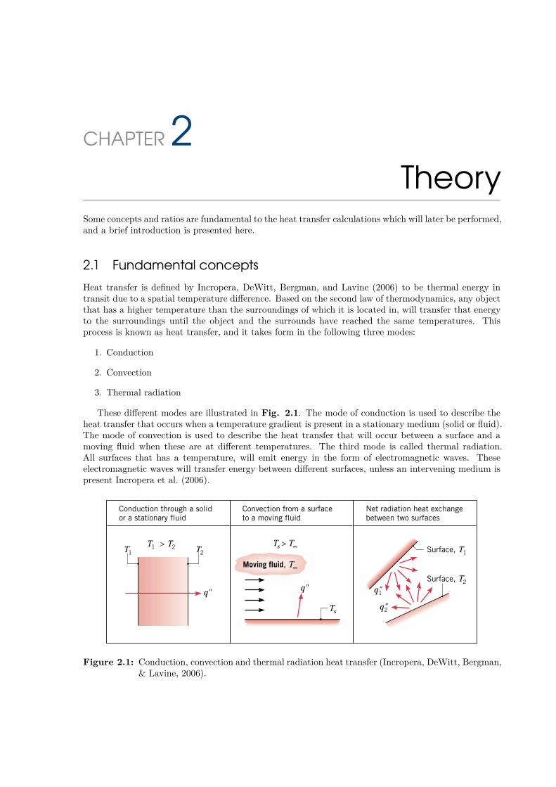
2.1 Fundamental conceptsHeat transfer is defined by Incropera, DeWitt, Bergman, and Lavine (2006) to be thermal energy intransit due to a spatial temperature difference. Based on the second law of thermodynamics, any objectthat has a higher temperature than the surroundings of which it is located in, will transfer that energyto the surroundings until the object and the surrounds have reached the same temperatures. Thisprocess is known as heat transfer, and it takes form in the following three modes:
1. Conduction
2. Convection
3. Thermal radiation
These different modes are illustrated in Fig. 2.1. The mode of conduction is used to describe theheat transfer that occurs when a temperature gradient is present in a stationary medium (solid or fluid).The mode of convection is used to describe the heat transfer that will occur between a surface and amoving fluid when these are at different temperatures. The third mode is called thermal radiation.All surfaces that has a temperature, will emit energy in the form of electromagnetic waves. Theseelectromagnetic waves will transfer energy between different surfaces, unless an intervening medium ispresent Incropera et al. (2006).
!"#$%"&'"!"!($"!)"!* )#!"$#! "+##!#!(,-#!"$#!"$"''+."!",/+&%!"#$"'+#!" 0$#!(+#$"!#!"$#!$$"!0&#!#! "#!$!$!#!(!" #!"$#!#""+#$#$$,-)1$#& #2#2!!"#$"!"'#( 34567 ""!* "!(&'0! '"#!$"'$'"""! 89:67;<!#$"0+'" !"#! $ "#"'"#!2,=)"##!(&"'>#!,?@9:A7@69::89B7C68DE4FA7@69::89B7C68865D?@GA7A:A3H48:9B:DI!)1$#&#&'0"!"00$#"#! !"!"'$!$0"!0#!$#0'"!'#""! 0$,J$!)1$#&##''""!!#!+#$".!+'( ""! ")+#K'"+ !"#$LM4B768N9:A4B4C6B68OGP'&0)''&"!$!'("!$#,QRQSTUU VWX J#0'%(!"'%K!##!0&# K$#!0!>#!Y="#""! Z=!&2#"0"# !$#!"#)+!#"%""! $$,J+!#![#(\,\%+ # !0 ""! 0$"34567;=!"0"("#!2##!""#!"#%+#$")"'#"]#%+M4B5M:A4B ""! "+#''$$"$#,<!$!"%M4BN6M:A4B ""!* "+#''$$)+!" "$"!"&#!(]#+!""# !E69::89B7C68_48@69:A7:@6839a6B68OGAB:89B7A:56:497H9:A9a:63H689:865ACC686BM6;bcbdbd bce fg fghijklmnoijnpqilrpstiuokiqstnsnoijsqvwulok hijxymnoijwqizstlqwsmyniszixojrwulok ynqskosnoijpysny|mpsjryyn~yyjn~itlqwsmytlqwsmybdlqwsmybcb7b b7 fgdfgcb ¡ ¢£ ¤¢¥Figure 2.1: Conduction, convection and thermal radiation heat transfer (Incropera, DeWitt, Bergman,
& Lavine, 2006).
12 2 Theory
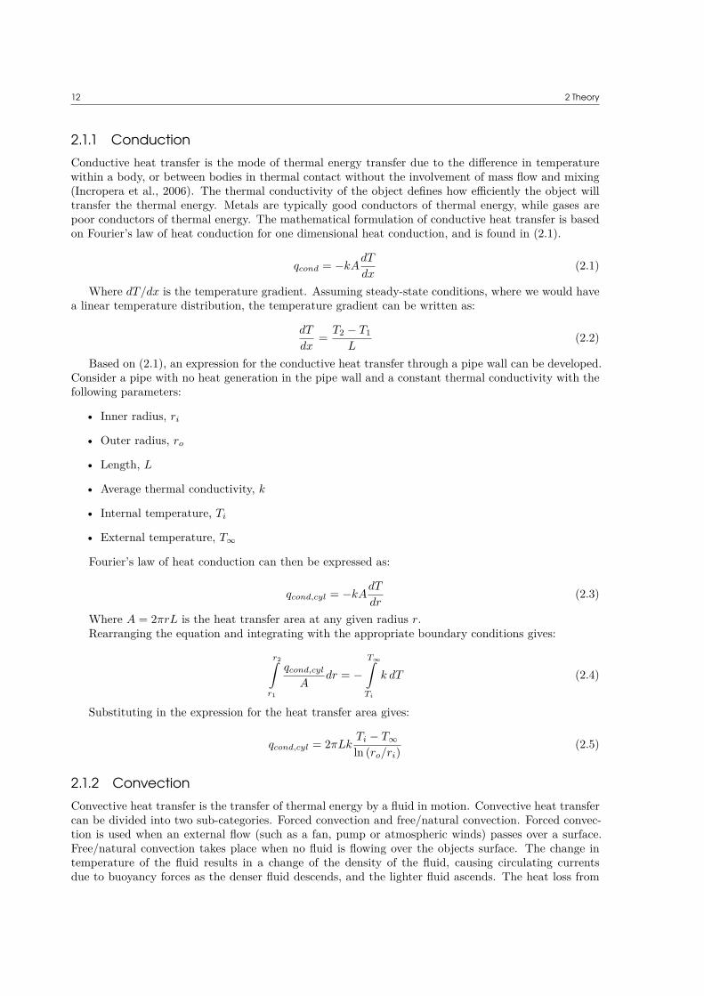
2.1.1 ConductionConductive heat transfer is the mode of thermal energy transfer due to the difference in temperaturewithin a body, or between bodies in thermal contact without the involvement of mass flow and mixing(Incropera et al., 2006). The thermal conductivity of the object defines how efficiently the object willtransfer the thermal energy. Metals are typically good conductors of thermal energy, while gases arepoor conductors of thermal energy. The mathematical formulation of conductive heat transfer is basedon Fourier’s law of heat conduction for one dimensional heat conduction, and is found in (2.1).
qcond = −kAdT
dx(2.1)
Where dT/dx is the temperature gradient. Assuming steady-state conditions, where we would havea linear temperature distribution, the temperature gradient can be written as:
dT
dx= T2 − T1
L(2.2)
Based on (2.1), an expression for the conductive heat transfer through a pipe wall can be developed.Consider a pipe with no heat generation in the pipe wall and a constant thermal conductivity with thefollowing parameters:
• Inner radius, ri
• Outer radius, ro
• Length, L
• Average thermal conductivity, k
• Internal temperature, Ti
• External temperature, T∞
Fourier’s law of heat conduction can then be expressed as:
qcond,cyl = −kAdT
dr(2.3)
Where A = 2πrL is the heat transfer area at any given radius r.Rearranging the equation and integrating with the appropriate boundary conditions gives:
r2∫r1
qcond,cyl
Adr = −
T∞∫Ti
k dT (2.4)
Substituting in the expression for the heat transfer area gives:
qcond,cyl = 2πLkTi − T∞
ln (ro/ri)(2.5)
2.1.2 ConvectionConvective heat transfer is the transfer of thermal energy by a fluid in motion. Convective heat transfercan be divided into two sub-categories. Forced convection and free/natural convection. Forced convec-tion is used when an external flow (such as a fan, pump or atmospheric winds) passes over a surface.Free/natural convection takes place when no fluid is flowing over the objects surface. The change intemperature of the fluid results in a change of the density of the fluid, causing circulating currentsdue to buoyancy forces as the denser fluid descends, and the lighter fluid ascends. The heat loss from

2.1 Fundamental concepts 13
free/natural convection can be observed in the experimental data, but will not be subject to calculationin this thesis. The mathematical formulation for convective heat transfer rate is found in (2.6).
qconv = hA (Ti − T∞) = Ts − T∞
1hA
(2.6)
Where:
• Convective heat transfer coefficient, h
• Surface area, A
• Surface temperature, Ts
• External / free-stream temperature, T∞
From (2.6), the relationship to the average heat transfer coefficient is established. The differencebetween h and h is that the latter takes the average surface conditions, whilst the first takes the localsurface conditions.
The average heat transfer coefficient can be written as:
h = qconv
A(Ts − T∞)(2.7)
2.1.3 Thermal radiationThermal radiation is energy emitted by any object that is at a non-zero temperature (Incropera et al.,2006). The mathematical formulation for net radiation heat transfer rate is found in (2.8).
qrad = εσA(Ti
4 − T∞4) (2.8)
Where:
• Factor, dependant on geometry and surface properties, ε
• Stefan-Boltzmann constant, σ
• Surface area, A
• Internal temperature, Ti
• External temperature, T∞
2.1.4 Thermal resistanceMany physical phenomena can be described by the general rate equation showed in (2.9) (Serth, 2007).
Flow rate = Driving forceResistance (2.9)
This general rate equation is used in Ohm’s Law of Electricity, shown in (2.10).
I = V
Re(2.10)
The same principle can be applied for heat transfer. For heat transfer, the flow rate is heat, orthermal energy. The driving force is the temperature difference between the object and the surroundings,and the resistance will be the thermal resistance, denoted by Rth. Based on this we get (2.11), whichwill be the foundation for the heat transfer calculations introduced later.

14 2 Theory
q = dT
Rth(2.11)
The concept of thermal resistance can help to greatly simplify otherwise complex heat transferproblems. As it is based on the same principles as Ohm’s Law, the thermal resistances can be combinedin the same way as electrical resistances.
Thus, for resistances in series, the total resistance is given by (2.12). For resistances in parallel, thetotal resistance is given by (2.13).
Rtot =∑
i
Ri (2.12)
Rtot =
(∑i
(1
Ri
))−1
(2.13)
An example of how this can be utilized is found in Fig. 2.2. Here, the cross-section of a compositematerial is shown. A total of four different materials are used, each with different thermal resistances.
Figure 2.2: Heat transfer through a composite material (Serth, 2007).
The total thermal resistance is given by:
Rth,tot = RA + RBC + RD
Where RBC is given by:
RBC =(
1RB
+ 1RC
)−1
= RBRC
RB + RC
When considering the concept of thermal resistance, the equations previously listed can be rewrittento facilitate their usage in radial coordinates. For conduction, (2.5) can be written as:
qcond,cyl = T1 − T2
Rcond,cyl(2.14)
Where Rcond,cyl is the thermal resistance of the cylindrical layer, given as:
Rcond,cyl = ln (r2/r1)2πLk
(2.15)
Similarly, for convection, we can rewrite (2.6) as:
qconv,cyl = T1 − T2
Rcond,cyl(2.16)
It follows that Rconv,cyl is given as:
Rconv,cyl = 12πrLh
(2.17)
2.1 Fundamental concepts 15
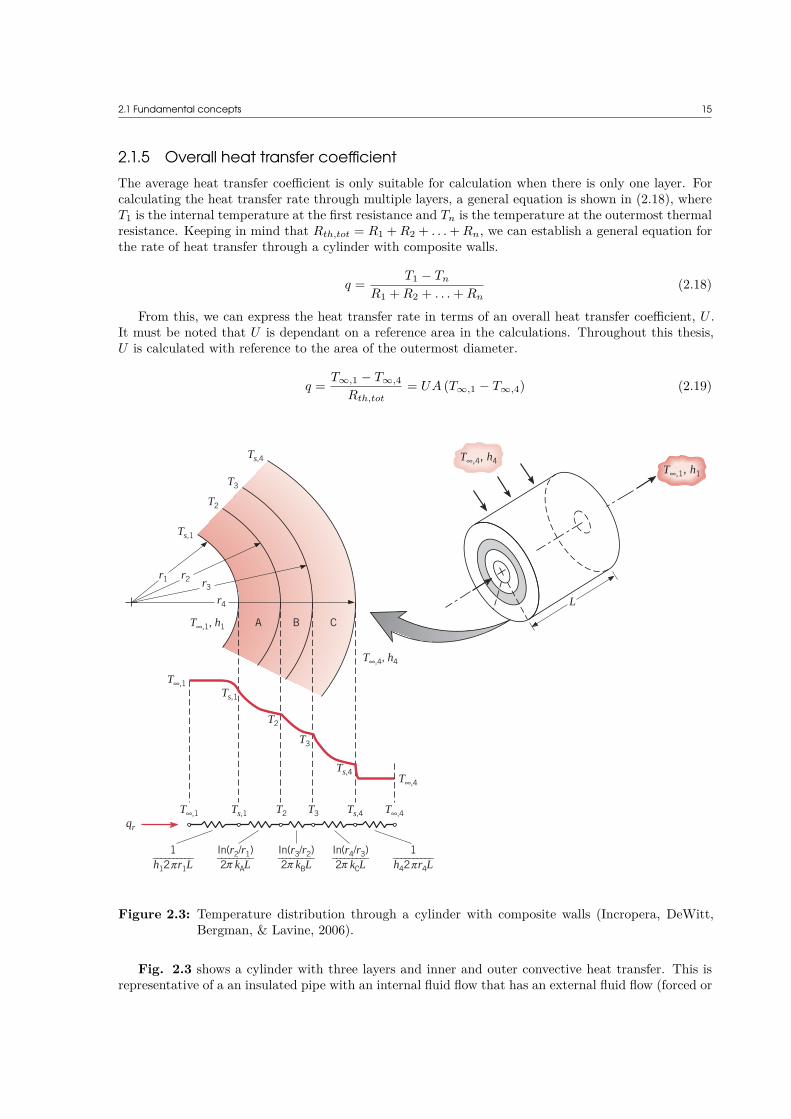
2.1.5 Overall heat transfer coefficientThe average heat transfer coefficient is only suitable for calculation when there is only one layer. Forcalculating the heat transfer rate through multiple layers, a general equation is shown in (2.18), whereT1 is the internal temperature at the first resistance and Tn is the temperature at the outermost thermalresistance. Keeping in mind that Rth,tot = R1 + R2 + . . . + Rn, we can establish a general equation forthe rate of heat transfer through a cylinder with composite walls.
q = T1 − Tn
R1 + R2 + . . . + Rn(2.18)
From this, we can express the heat transfer rate in terms of an overall heat transfer coefficient, U .It must be noted that U is dependant on a reference area in the calculations. Throughout this thesis,U is calculated with reference to the area of the outermost diameter.
q = T∞,1 − T∞,4
Rth,tot= UA (T∞,1 − T∞,4) (2.19)118 Chapter 3 One-Dimensional, Steady-State Conduction
Consider now the composite system of Figure 3.7. Recalling how we treatedthe composite plane wall and neglecting the interfacial contact resistances, the heattransfer rate may be expressed as
(3.29)
The foregoing result may also be expressed in terms of an overall heat transfer coef-ficient. That is,
(3.30)
If U is defined in terms of the inside area, A1 2r1L, Equations 3.29 and 3.30 maybe equated to yield
(3.31)
This definition is arbitrary, and the overall coefficient may also be defined in termsof A4 or any of the intermediate areas. Note that
(3.32)U1A1 U2A2 U3A3 U4A4 (Rt)1
U1 1
1h1
r1
kAln
r2r1
r1
kBln
r3r2
r1
kCln
r4r3
r1r4
1h4
qr T,1 T,4
Rtot UA(T,1 T,4)
qr T,1 T,4
12r1Lh1
ln (r2/r1)2kAL
ln (r3/r2)2kBL
ln (r4/r3)2kCL
1
2r4Lh4
qr
T∞,4
Ts,4
T3
T2
Ts,1
T∞,1
T∞,1 T∞,4Ts,1 T2 T3 Ts,4
1__________h12 r1L
In(r2/r1)_________2 kALπ π
In(r3/r2)_________2 kBLπ
In(r4/r3)_________2 kCLπ
1__________h42 r4Lπ
A B C
r1 r2 r3
r4
T∞,1, h1
T∞,4, h4
Ts,1
T2
T3
Ts,4 T∞,4, h4T∞,1, h1
L
FIGURE 3.7 Temperature distribution for a composite cylindrical wall.Figure 2.3: Temperature distribution through a cylinder with composite walls (Incropera, DeWitt,
Bergman, & Lavine, 2006).
Fig. 2.3 shows a cylinder with three layers and inner and outer convective heat transfer. This isrepresentative of a an insulated pipe with an internal fluid flow that has an external fluid flow (forced or

16 2 Theory
free convection). Layer A is the pipe wall, layer B is the layer of insulation and layer C is a protectivetube around the insulation.
The equation for the heat transfer rate for this configuration is shown in (2.20).
q =T∞,1 − T∞,4
1h12πr1L
+ln (r2/r1)
2πkAL+
ln (r3/r2)2πkBL
+ln (r4/r3)2πkCL
+1
h42πr4L
(2.20)
As the heat transfer rate is constant throughout the cylinder, we can also express q as shown in(2.21).
q =T∞,1 − Ts,1
1h12πr1L
=Ts,1 − T2
ln (r2/r1)2πkAL
=T2 − T3
ln (r3/r2)2πkBL
=T3 − Ts,4
ln (r4/r3)2πkCL
=Ts,4 − T∞,4
1h42πr4L
(2.21)
The relationship in (2.21) will be used later to calculate the surface temperature of the insulationin order to evaluate the fluid properties.
2.1.6 Nusselt numberThe Nusselt number is a dimensionless temperature gradient at the surface, and provides a measure ofthe convection coefficient, or the ratio of convection to pure conduction heat transfer (Incropera et al.,2006). The Nusselt number is defined in (2.22), where D is the characteristic length (diameter) of thesurface of interest.
NuD = hD
k(2.22)
2.1.7 Prandtl numberThe Prandtl number is the ratio of momentum diffusivity and thermal diffusivity. It provides a measureof the relative effectiveness of momentum and energy transport by diffusion in the velocity and thermalboundary layers (Incropera et al., 2006). The definition of the Prandtl number is found in (2.23).
Pr = cpµ
k= ν
α(2.23)
2.1.8 Reynolds numberThe Reynolds number is the ratio of inertia to viscous forces, and can be used to characterize flowsat the boundary layer (Moran, Shapiro, Munson, & DeWitt, 2003). The definition of the Reynoldsnumber is found in (2.24), where D is the characteristic length (diameter) of the surface of interest.
ReD ≡ ρu∞D
µ= u∞D
ν(2.24)
When calculating the behaviour of the boundary layer, the transition between laminar and turbulentflow takes place at an arbitrary location xc, as shown in Fig. 2.4. This location is determined by thecritical Reynolds number, Rex,c and varies from 105 to 3 × 10⁶, depending on surface roughness andturbulence level of the free-stream (Incropera et al., 2006). A representative value of 5×10⁵ is frequentlyused, and will be used in this thesis. For reference, the definition of the critical Reynolds number isfound in (2.25).
Rex,c ≡ ρu∞xc
µ(2.25)
(2.25) can be rewritten to give the distance xc, where the transition takes place:

2.1 Fundamental concepts 17
xc = ν
u∞Rexc (2.26)
2.1.9 Film temperatureTo account for the variations of the thermodynamic properties with temperature, the term film temper-ature has been developed (Çengel, 2006). The film temperature is defined as the arithmetic mean ofthe surface and free-stream (ambient) temperatures, and can be found in (2.27). When using the filmtemperature, the fluid properties are assumed to be constant during the entire flow.
Tf = Ts + T∞
2(2.27)
2.1.10 Dynamic viscositySutherland (1893) presented a relationship between the dynamic viscosity and the absolute temperatureof an ideal gas. This has later been adopted and updated, and from Sutherland’s law (2008) we havethe equation shown in (2.28) for calculating the dynamic viscosity of air at different temperatures.
µ = µref
(T
Tref
)3/2(Tref + S
T + S
)(2.28)
Where Tref is the reference temperature, µref is the dynamic viscosity at Tref and S is Sutherland’sconstant for the gas of interest. For air, the following constants are known:
Table 2.1: Constants for use with Sutherland’s law (2.28).
Variable ValueS = 110.4K
Tref = 273.15Kµref = 17.16 × 10⁻⁶N · s/m2
2.1.11 Kinematic viscosityThe kinematic viscosity is the ratio of the dynamic viscosity, µ to the density of the fluid, ρ. Thedynamic viscosity can be assumed to remain constant, while the density of a gas will very dependingon temperature and pressure. The density of air at a certain temperature is given in (2.29). This canthen be used to establish the kinematic viscosity of the gas using (2.30).
ρ = p
Rair ∗ T(2.29)
ν = µ
ρ(2.30)
2.1.12 Thermal diffusivityThe thermal diffusivity of a material characterizes the ratio of the thermal conductivity to the heatcapacity. A large value of α indicates that the material will respond quickly to temperature changes,while a low value of α indicates that the material will respond more sluggishly, and will take longer toreach equilibrium (Incropera et al., 2006).
α = k
ρcp(2.31)

18 2 Theory
2.2 Heat transfer correlations
2.2.1 Forced flow over a flat plateWhen considering the heat transfer for a flat plate subjected to forced flow, it is important to understandhow the wind develops over the surface. The different states of the flow is presented in Fig. 2.4. Initially,a laminar flow is dominating. This flow changes to a transitional flow, until it reaches a final, turbulentflow. From Incropera et al. (2006) we have two different equations to calculate the Nusselt number atthe different states. For laminar flow, (2.32) is used. For transitional and turbulent flows (2.33) is used.
NuD = hDD
k= 0.664Re1/2
D Pr1/3 (2.32)[Pr ≥ 0.6
]
NuD =(
0.037Re4/5D − A
)Pr1/3 (2.33)[
0.6 ≤ Pr ≤ 60Rex,c ≤ ReD ≤ 108
]Where A is a constant determined by the critical Reynolds number Rex,c. The calculation for A is
found in (2.34). For Rex,c = 5 × 10⁵, A = 867.
A = 0.037Re4/5x,c − 0.664Re1/2
x,c (2.34)
! "#$%"!"#& " '()*+),-./.),012"3 #4#"5 "6!4#735#5%#7"#63"6#(89.,8:#/;:<;(=,/1># " #"!#" ##"4#&36% ?1@ ABCDEBFBEGHIFJIKLEMNLKOPDMQROIEGBFQABQLFST"#63"6#-=U=()V9=,/" 3"43"33#"WX15"6"$3"5"#"#73 3%7#$%3"5"#4#˛W##$ 35"#"#Y76!3Z654[Z"\Z#1W35"%"6 #5# ""763%& 3"#%"33"7"#63"6#&#%[Z#1WX%"#"#"#4 #7%3"5"#"#73 3%$"#7 33%&4"#"&#"413"5"#7"#63"6#$ 3 3%&36##"473 6#"53"3&% 34"#35!1W#5>X1]1]%%"7"#63"6#&#%""!36&#""\_`#"#"5%a#"&[b#1W#5cd"X1e$%"3"3# ""##f0"3#"%#"&[1g&36##7"!#3"/:8,0./.),Y#"$"#%"!# #53"5"##73#1h%#"Y"&%5$% 3%55?7&3"5"#7"!#"5Z5?7&"#"# #73 3%1W3% 336#737"#63"6#$&#"3$&36##&3"#""#"#Y76#"5$#Z5"35 #3"!363"#&4"#3 31i?&%7"#63"6#"##&Z4 3%"#3# ""#" #3%#Z5!& 3 "## ##"51i
jklm lno
pqrstujkj vwxyz|~yxwwwxyw|yx|x|w ;; ;[;\ ; [+ [ Figure 2.4: Velocity boundary layer development over a flat plate (Incropera, DeWitt, Bergman, &
Lavine, 2006).
2.2.2 Forced flow over a cylinder in cross-windTo calculate the convective heat transfer coefficient for a cylinder in cross-flow, a correlation must beused. There are numerous correlations that can be used, with different ranges of validity and accuracy.

2.2 Heat transfer correlations 19
Moran et al. (2003) states that the expected accuracy is no more than ±25 − 30%. Incropera et al.(2006) is more optimistic, and suggests an expected accuracy of ±20%.
Numerous comparisons of the different correlations have been performed. Morgan (1975) did acomprehensive review of the existing literature on convective heat transfer. Manohar and Ramroop(2010) performed a comparison of five different correlations using experimental data on pipes at differentwind speeds and inclinations of a pipe, although their findings might not be accurate as mistakes werefound in the constants used for some of the correlations. Whitaker (1972) performed a comprehensivereview as well, and presents comparative plots of the different correlations.
2.2.2.1 Hilpert correlation
The Hilpert correlation was suggested in Hilpert (1933), and has proven to be quite good estimate forthe average Nusselts number over a pipe in a cross-flow arrangement. The Hilpert correlation is anempirical correlation, and has the form found in (2.35) (Çengel, 2006; Incropera et al., 2006; Moranet al., 2003). The constants initially proposed by Hilpert are found in Tab. 2.2, but have since beenrevised and recalculated, as new and more accurate thermodynamic data has emerged. The constantspresented in Tab. 2.3 are recommended for use by Çengel (2006), Incropera et al. (2006), Moran et al.(2003). All properties in Tab. 2.3 are evaluated at the film temperature.
NuD = C RemD Pr1/3 (2.35)[
Pr ≥ 0.7]
Table 2.2: Constants originally proposed by Hilpert (1933).
ReD C m1 - 4 0.891 0.3304 - 40 0.821 0.385
40 - 4 000 0.615 0.4664 000 - 40 000 0.174 0.618
40 000 - 400 000 0.0239 0.805
Table 2.3: Updated constants for use with the Hilpert correlation (Çengel, 2006; Incropera, DeWitt,Bergman, & Lavine, 2006; Moran, Shapiro, Munson, & DeWitt, 2003).
ReD C m0.4 - 4 0.989 0.3304 - 40 0.911 0.385
40 - 4 000 0.683 0.4664 000 - 40 000 0.193 0.618
40 000 - 400 000 0.027 0.805
Based on Hilpert’s work, Fand and Keswani (1973) recalculated the constants used in Hilpert’scorrelation based on more accurate values for the thermodynamic properties of air than what wasavailable in 1933. All temperatures are evaluated at film temperature. The constants proposed by Fandand Keswani (1973) are presented in Tab. 2.4.
Morgan (1975) recalculated the constants used in the Hilpert correlation based on an extensivereview of existing literature on convective heat transfer. The recalculated values are found in Tab.2.5.

20 2 Theory
Table 2.4: Reviewed values of C and m (Fand & Keswani, 1973).
ReD C m1 - 4 0.875 0.3134 - 40 0.785 0.388
40 - 4 000 0.590 0.4674 000 - 40 000 0.154 0.627
40 000 - 400 000 0.0247 0.898
Table 2.5: Reviewed values of C and m (Morgan, 1975).
ReD C m0.0001 - 0.004 0.437 0.08950.004 - 0.09 0.565 0.136
0.09 - 1 0.800 0.2801 - 35 0.795 0.384
35 - 5 000 0.583 0.4715 000 - 50 000 0.148 0.633
50 000 - 200 000 0.0208 0.814
2.2.2.2 Žukauskas correlation
Žukauskas (1972) presents the correlation found in (2.36). In this, all properties are evaluated at thefree-stream (ambient) temperature, except for Prs, which is evaluated at the surface temperature.
NuD = CReDmPrn
(PrPrs
)1/4
(2.36)[0.7 ≤ Pr ≤ 5001 ≤ ReD ≤ 106
]The constants used are presented in Tab. 2.6 & 2.7.
Table 2.6: Values of n for different Prandtl numbers (Žukauskas, 1972).
Pr n
< 10 0.37≥ 10 0.36
Table 2.7: Suggested values of C and m (Žukauskas, 1972).
ReD C m1 - 40 0.75 0.4
40 - 1 000 0.51 0.51 000 - 200 000 0.26 0.6
200 000 - 1 000 000 0.076 0.7
2.2.2.3 Whitaker correlation
Whitaker (1972) presents the correlation found in (2.37).

2.3 Time to freeze 21
NuD =(
0.5Re1/2D + 0.06Re
2/3D
)Pr0.4
(µb
µs
)1/4
(2.37)[1.00 ≤ Re ≤ 1 × 10⁵
0.67 ≤ Pr ≤ 300
]Where:
• µb is the fluid viscosity at bulk temperature (same as free-stream temperature for open systems).
• µs is the fluid viscosity at surface temperature.
Whitaker (1972) notes that this correlation is generally within ±25% of other correlations, except atlow Reynolds numbers, where the Hilpert correlation gives considerably higher values.
2.2.2.4 Churchill-Bernstein correlation
Churchill and Bernstein (1977) presents the correlation found in (2.38) and had as a goal to provide asingle, comprehensive equation for the heat transfer coefficient of a cylinder subjected to a cross-flowwind, for all ranges of Reynolds numbers, and a wide range of Prandtl numbers. All fluid propertiesare evaluated at film temperature.
NuD = 0.3 + 0.62Re1/2Pr1/3[1 + (0.4/Pr)2/3
]1/4 ×
[1 +
(Re
282000
)5/8]4/5
(2.38)
[ReDPr ≥ 0.2
]2.2.2.5 Discussion
The Žukauskas and the Churchill-Bernstein correlation are recommended by Incropera et al. (2006)as they are valid for a wide range of conditions and are the most recent ones. Moran et al. (2003)recommends the use of the Churchill-Bernstein correlation unless the simplicity of the Hilpert is advan-tageous. Theodore (2011) recommends the Hilpert correlation, while Çengel (2006) recommends theChurchill-Bernstein correlation.
As the wind speeds experienced for winterization purposes can be expected to be lower than 20m/s in most applications, the critical dimension will be the diameter. For wind speeds lower than 20m/s, pipes with an outer diameter of less than 1.0 m, the Reynolds number will not exceed 400 000.This means that all correlations apart from the Hilpert correlation with Morgan’s constants and theWhittaker correlation are valid. Morgan’s constants have a limit at Re ≤ 200000, and the Whittakercorrelation have a limit at Re ≤ 100000. These correlation will therefore not be one of the correlationswhich will be considered for recommendation, but will still be compared in the theoretical calculations.
In general, all of the correlations have different ranges of applicability and some are likely to bemore accurate at certain ranges. None of the correlations are particularly difficult to implement inMATLAB, Python or Microsoft Excel, so the choice of correlation will depend on the accuracy foundin the expected range of operation. It is however noted that the empirical correlation based on Hilpert(1933) is easier to use for hand-calculations due to the simplicity of the equation, but the availabilityof computers and powerful hand-held devices has reduced the importance of this.
2.3 Time to freezeThe time to freeze calculations are quite different from the other calculations, and will be presented here.The calculations made in Kvamme (2014) assumed a constant heat flux throughout the freezing process,

22 2 Theory
and was not suitable for more detailed calculations. ASHRAE (2010, ch: 19-20) presents methods usedfor calculating the freezing time of foods and beverages. One of these methods is adopted for pipesin this thesis, and were found to give reasonable values. The following methodology is suggested byASHRAE (2010):
1. Determine thermal properties
2. Determine surface heat transfer coefficient
3. Determine characteristic dimensions and ratios
4. Calculate Biot, Plank and Stefan numbers
5. Calculate the freezing time for an infinite slab
6. Calculate the equivalent heat transfer dimensionality
7. Calculate the freezing time
It is noted that ASHRAE (2010) presents several different methods and correction factors for calcu-lating the required time to freeze. Some of the methods might be more applicable and accurate for thetime to freeze depending on the scenario, and it is recommended to consult ASHRAE (2010) if similarcalculations will be performed.
2.3.1 Biot numberThe Biot number is the ratio of the external heat transfer resistance to the internal heat transferresistance, as shown in (2.39) (ASHRAE, 2010).
Bi = hextL
k(2.39)
Where:
• hext is the convective heat transfer coefficient
• L is the characteristic dimension of object
• k is the thermal conductivity of the object
2.3.2 Plank numberThe Plank number is defined as the ratio between the volumetric specific heat of the unfrozen phaseand the volumetric enthalpy change. The equation for the Plank number is given in (2.40) (ASHRAE,2010).
Pk = Cl (Ti − Tf )∆H
(2.40)
2.3.3 Stefan numberThe Stefan number is similar to the Plank number, but gives the ratio between the volumetric specificheat of the frozen phase and the volumetric enthalpy change. The equation for the Stefan number isfound in (2.41) (ASHRAE, 2010).
Ste = Cs (Tf − T∞)∆H
(2.41)

2.3 Time to freeze 23
2.3.4 Volumetric specific heatThe volumetric specific heat is measure of the specific heat of the object per unit volume, and is givenas the density of the object multiplied by the heat capacity of the object, as shown in (2.42) (ASHRAE,2010).
C = ρc (2.42)
2.3.5 Volumetric enthalpyThe volumetric enthalpy is the difference between the object at the initial temperature in unfrozen stateand the final temperature in solid state. From ASHRAE (2010) we have the equation in (2.43).
∆H = ρlHl − ρsHs (2.43)
Where:
• ρl is the density of the object in a liquid state
• Hl is the enthalpy of the object at initial temperature in liquid state
• ρs is the density of the object in a solid state
• Hs is the enthalpy of the object at the final temperature in solid state
In the calculations, it is assumed that the enthalpy of water in liquid state is given by:
ρl = Hf + (cwaterTi) (2.44)
Similarly, for the solid state:
ρs = ciceTf (2.45)
Where:
• Hf is the enthalpy of fusion for water
• cwater is the heat capacity of water
• Ti is the initial temperature of water
• cice is the heat capacity of ice
• Tf is the final temperature of ice
2.3.6 Characteristic dimensionsThe characteristic dimension used is twice the shortest distance from the thermal center of the objectto the surface. For a cylinder, this is equal to the diameter of the cylinder.
Lcyl = D (2.46)
Depending on the shape of the object, the dimensional ratios β1 and β2 will vary.The general definitions are:

24 2 Theory
β1 = Second shortest dimension of objectShortest dimension of object (2.47)
β2 = Longest dimension of objectShortest dimension of object (2.48)
For a finite cylinder, these dimensional ratios are the same, and is calculated using (2.49).
β1cyl = β2cyl = L
D(2.49)
2.3.7 Freezing time of infinite slabTo calculate the freezing time of an infinite slab, the method presented by Hung and Thompson (1983)is used.
The weighted average temperature difference is found in (2.50).
∆T = (Tf − T∞) +(Ti − Tf )2
(Cl
2
)− (Tf − Tc)2
(Cs
2
)∆H
(2.50)
Geometric properties of the shape and the infinite slab for use in the equations are found in (2.51).
U = ∆T
Tf − T∞(2.51)
P = 0.7306 − (1.083Pk) + Ste
((15.4U) − 15.43 +
(0.01329
(SteBi
)))(2.52)
R = 0.2079 − 0.2656USte (2.53)
The time to freeze an infinite slab is found in (2.54).
θslab = ∆H × 103
∆T
[PD
hext+ RD2
ks
](2.54)
2.3.8 Equivalent heat transfer dimensionalityThe time to freeze for a specific shape is found by dividing the time to freeze the infinite slab by theequivalent heat transfer dimensionality, E as shown in (2.55).
θcyl = θslab
E(2.55)
E is given in (2.56).E = G1 + G2E1 + G3E2 (2.56)
Where G1, G2 and G3 are geometric constants which vary depending on the specific shape. For afinite cylinder with L > D, G1 = 2, G2 = 0 and G3 = 1.
E2 is found in (2.57), where X and Φ is given in (2.58) and (2.59) respectively
E2 = X (Φ)β2
+ [1 − X (Φ)] 0.5β2
3.69 (2.57)
X (Φ) = ΦBi1.34 + Φ
(2.58)

2.3 Time to freeze 25
Φ = 2.32β2
1.77 (2.59)

26

CHAPTER 3Calculations
In this chapter, an example of the theoretical calculations will be performed. These calculations arethe same as the calculations that is used for tables and comparisons in Chapter 5. The time to freezeis calculated using the Python program, the code for which is found in Appendix B.
3.1 Forced flow over a flat plateFor this example, a calculation of the required amount of heating to keep a 1.1 m x 1.1 m plate at asteady surface temperature of +5 C, when subjected to a 10 m/s wind from one direction. Ambienttemperature is −20 C. These conditions are representative of Experiment 12. The constants used arelisted in Tab. 3.1.
The following assumptions are made:
1. Steady-state conditions.
2. The heat transfer coefficient is uniform across the plate.
3. Material properties are constant.
4. One-dimensional heat transfer.
5. 90 % of the consumed electrical power is converted to heat.
6. Critical Reynolds number, Rex,c = 5 × 10⁵.
7. Pallet used is 120 cm x 80 cm x 15 cm (L x W x H).
8. 80 % of the pallet area is in contact with the deck element.
9. Temperature of pallet is equal to ambient temperature.
10. Air flow over bottom surface of deck element is in laminar regime.
11. Negligable differences in thermodynamic properties of air at temperature range.
12. The surface temperature of the plate is uniform and constant.
13. The deck element has a uniform height across the surface.
3.1.1 Conductive heat transferConductive heat transfer takes place from the underside of the deck element to the pallet. This heattransfer can be calculated using (2.1):
qcond = −kAdT
dx(3.1)

28 3 Calculations
Table 3.1: Constants used in calculations for flat plate.
Variable Description Value UnitL Length 1.1 mW Width 1.1 mh Height of deck element 3.0 cm
Apc Area of pallet in contact with deck element 0.768 mtw Thickness of wood planks on pallet 3.0 cmT∞ Ambient temperature −20 CTs Surface temperature +5 Cu∞ Wind speed 10 m/s
patm Atmospheric pressure 101.3 kPaε Emissivity of plate at 300 K 0.93 N/A
kair Thermal conductivity of air at 250 K 2.23 × 10⁻² W/m · Kkwood Thermal conductivity of wood at 250 K 0.15 W/m · Kαair Thermal diffusivity of air at 250 K 1.59 × 10⁻⁵ m2/sµair Dynamic viscosity of air at 250 K 1.596 × 10⁻⁵ N · s/m2
ρair Density of air at 250 K 1.395 kg/m3
qpallet = kwood × Apc ×(
Ts − T∞
tw
)= 0.15 × 0.768 ×
(278.15 − 253.15
0.03
)= 96.0W
(3.2)
3.1.2 Convective heat transferFrom (2.6), the relationship for the convective heat transfer:
q = hA (Ts − T∞) (3.3)
The kinematic viscosity of air is found from (2.30):
νair,∞ = µair,∞
ρair,∞
= 1.596 × 10⁻⁵
1.395= 1.14 × 10⁻⁵m2/s
(3.4)
Prandtl number, from (2.23):
Prair,∞ = νair,∞
αair,∞
= 1.14 × 10⁻⁵
1.596 × 10−5
= 0.717
(3.5)

3.1 Forced flow over a flat plate 29
Reynolds number, from (2.24):
Reair,∞ = u∞D
νair,∞
= 10 × 1.11.14 × 10−5
= 961259.4
(3.6)
This is higher than the critical Reynolds number, so a combination of laminar and turbulent flow isassumed.
Calculate the distance, xc from the edge to where the transition from laminar to turbulent flowoccurs:
xc = ν
u∞Rexc
= 1.14 × 10⁻⁵
15× 5 × 105
= 0.572m
(3.7)
Calculate the Nusselt number for laminar flow from (2.32) and turbulent flow (2.33), respectively.
Nulam = 0.664Re1/2D Pr1/3
= 0.664 × 961259.41/2 × 0.7171/3
= 582.68(3.8)
Nuturb = (0.037Re4/5D − A)Pr1/3
= 0.037 ×(
961259.44/5 − 867)
× 0.7171/3
= 1248.49
Find h using the relationship in (2.32):
NuD = hDD
k
hD = NuDk
D
(3.9)
Inserting the values calculated for the Nusselt number:
hlam = 582.68 × 2.23 × 10−2
1.1= 11.81W/m2 · K
(3.10)
hturb = 1248.49 × 2.23 × 10−2
1.1= 25.31W/m2 · K
Calculate the heat transfer rate for the laminar and turbulent regimes of the plate with (3.3).

30 3 Calculations
qtop,lam = hlamA (Ts − T∞)= 11.81 × (0.572 × 1.1) × (278.15 − 253.15)= 185.86W
qtop,turb = hturbA (Ts − T∞)= 25.31 × (0.528 × 1.1) × (278.15 − 253.15)= 367.39W
(3.11)
Similarly, the heat transfer rate can be found for the sides of the deck element:
qsides,lam = hlamA (Ts − T∞)= 11.81 × (4 × 0.03 × 1.1) × (278.15 − 253.15)= 38.98W
(3.12)
And for the underside of the deck element, as the deck element was subjected to wind on both sidesduring testing:
qbottom,lam = hlamA (Ts − T∞)= 11.81 × ((1.1 × 1.1) − 0.768) × (278.15 − 253.15)= 130.52W
(3.13)
3.1.3 Thermal radiationWe can also include the heat loss due to thermal radiation. The area used includes the top and bottomsurfaces. From (2.8) we have:
qrad = εσA(Ti
4 − T∞4) (3.14)
Inserting values, we get:
qrad = 0.93 × 5.6704 × 10−8 × ((2 × 1.1 × 1.1) − 0.768 + (4 × 0.03 × 1.1)) ×((278.15)4 − (253.15)4)
= 176.75W
(3.15)
3.1.4 Total power consumptionThe total heating requirement will thus be:
qtot = qpallet + qtop,lam + qtop,turb + qsides + qbottom + qrad
= 96.0 + 185.86 + 367.39 + 38.98 + 130.52 + 176.75= 995.2W
(3.16)
Assuming a 90% efficiency of the heating element, the total electrical power will be:
η = qtot
qelec
qelec = qtot
η
= 995.2W
0.9= 1106.11W
(3.17)

3.2 Forced flow over an insulated pipe 31
3.1.4.1 Comments
The power consumption calculations performed here are based largely on assumptions, and should beused with care.
3.2 Forced flow over an insulated pipeIn this scenario we will consider an pipe with an outer diameter of 50 mm, with 10 mm Armaflexinsulation. The pipe is exposed to 15 m/s cross-wind at −20 C air temperature. Constants used in thecalculations are listed in Tab. 3.2. The overall heat transfer coefficient is calculated with respect tothe outer area of the pipe.
Assumptions:
1. Steady-state conditions.
2. The heat transfer coefficient is uniform across the pipe.
3. Material properties are constant.
4. One-dimensional heat transfer in radial direction.
5. 90 % of the consumed electrical power is converted to heat.
6. The surface temperature of the pipe is uniform and constant.
7. The heat loss through the end caps is negligible.
8. Heat loss due to radiation is negligible.
Table 3.2: Constants used in calculations for insulated pipe.
Variable Description Value UnitL Length 1.04 mD Diameter 50 mm
tins Insulation thickness 10 mmT∞ Ambient temperature −20 C
Tpipe Pipe temperature 45 CTins Insulation temperature −15 Cu∞ Wind speed 15 m/sp Atmospheric pressure 101.3 kPa
αair Thermal diffusivity of air (at 250K) 1.59 × 10⁻⁵ m2/skair Thermal conductivity of air (at 250K) 2.23 × 10⁻² W/m · Kkins Thermal conductivity of insulation 3.30 × 10⁻² W/m · K
Thermodynamic properties of air at film temperature
The film temperature is calculated from (2.27):
Tf = Tins + T∞
2= 258.15 + 253.15
2= 255.65K
(3.18)

32 3 Calculations
Dynamic viscosity of air, from (2.28):
µair,f = 17.16 × 10⁻⁶N · s/m2(
T
273.15K
)3/2(273.15K + 110.4K
T + 110.4K
)= 17.16 × 10⁻⁶
(255.65273.15
)3/2(273.15 + 110.4255.65 + 110.4
)= 1.628 × 10⁻⁵N · s/m2
(3.19)
Density of air, from (2.29):
ρair,f = patm
Rair × T
= 101.30.287 × 255.65
= 1.381kg/m3
(3.20)
Kinematic viscosity of air, from (2.30):
νair,f = µ
ρ
= 1.628 × 10⁻⁵
1.381= 1.179 × 10⁻⁵m2/s
(3.21)
Prandtl number, from (2.23):
Prair,f = νair
αair
= 1.179 × 10⁻⁵
15.9 × 10−6
= 0.742
(3.22)
Reynolds number, from (2.24):
Reair,f = u∞D
νair,f
= 15 × (0.05 + 2 × 0.01)1.179 × 10−5
= 89044.13
(3.23)
Thermodynamic properties of air at surface temperature
Using the same method as for film temperature, the thermodynamic properties of air is found at thesurface temperature.
Dynamic viscosity of air:µair,s = 1.641 × 10⁻⁵N · s/m2 (3.24)
Density of air:ρair,s = 1.367kg/m3 (3.25)
Kinematic viscosity of air:νair,s = 1.200 × 10⁻⁵m2/s (3.26)
Prandtl number:Prair,s = 0.755 (3.27)
Reynolds number:Reair,s = 87497.47 (3.28)

3.2 Forced flow over an insulated pipe 33
Thermodynamic properties of air at free-stream temperature
Using the same method as for film temperature, the thermodynamic properties of air is found at thefree-stream temperature.
Dynamic viscosity of air:µair,∞ = 1.615 × 10⁻⁵N · s/m2 (3.29)
Density of air:ρair,∞ = 1.394kg/m3 (3.30)
Kinematic viscosity of air:νair,∞ = 1.158 × 10⁻⁵m2/s (3.31)
Prandtl number:Prair,∞ = 0.729 (3.32)
Reynolds number:Reair,∞ = 90635.58 (3.33)
The Nusselt number calculations will now be performed for all the correlations presented in section2.2.2.
3.2.1 Hilpert correlationFrom (2.35) we have:
NuD = CRemDPr1/3
air,f (3.34)[Pr ≥ 0.7
]3.2.1.1 Original Hilpert constants
From Tab. 2.2 we find C = 0.0239 and m = 0.805 for the Reynolds number calculated in (3.23).
NuD = 0.0239 × 89044.130.805 × 0.7421/3
= 208.72(3.35)
Find h using the relationship in (2.22):
hD = NuDkair
D
= NuDkair
D + 2 × tins
= 208.72 × 2.23 × 10−2
0.050 + 2 × 0.01= 66.49W/m2 · K
(3.36)
We can now find the overall heat transfer coefficient from (2.20):

34 3 Calculations
U1 = 1
Dins × ln
(Dins
Do
)2 × kins
+1he
= 1
0.070 × ln
(0.0700.050
)2 × (3.30 × 10−2)
+1
66.49= 2.69W/m2 · K
(3.37)
3.2.1.2 Updated Hilpert constants
From Tab. 2.3 we find C = 0.027 and m = 0.805 for the Reynolds number calculated in (3.23).
NuD = 0.027 × 89044.130.805 × 0.7421/3
= 235.79(3.38)
Find h using the relationship in (2.22):
hD = NuDkair
D
= NuDkair
D + 2 × tins
= 235.79 × 2.23 × 10−2
0.050 + 2 × 0.01= 75.12W/m2 · K
(3.39)
We can now find the overall heat transfer coefficient from (2.20):
U1 = 1
Dins × ln
(Dins
Do
)2 × kins
+1he
= 1
0.070 × ln
(0.0700.050
)2 × (3.30 × 10−2)
+1
75.12= 2.70W/m2 · K
(3.40)
3.2.1.3 Fand & Keswani constants
From Tab. 2.4 we find C = 0.0247 and m = 0.898 for the Reynolds number calculated in (3.23).
NuD = 0.0247 × 89044.130.898 × 0.7421/3
= 622.55(3.41)

3.2 Forced flow over an insulated pipe 35
Find h using the relationship in (2.22):
hD = NuDkair
D
= NuDkair
D + 2 × tins
= 622.55 × 2.23 × 10−2
0.050 + 2 × 0.01= 198.33W/m2 · K
(3.42)
We can now find the overall heat transfer coefficient from (2.20):
U1 = 1
Dins × ln
(Dins
Do
)2 × kins
+1he
= 1
0.070 × ln
(0.0700.050
)2 × (3.30 × 10−2)
+1
198.33= 2.76W/m2 · K
(3.43)
3.2.1.4 Morgan constants
From Tab. 2.5 we find C = 0.0208 and m = 0.814 for the Reynolds number calculated in (3.23).
NuD = 0.0208 × 89044.130.814 × 0.7421/3
= 201.27(3.44)
hD = NuDkair
D
= NuDkair
D + 2 × tins
= 201.27 × 2.23 × 10−2
0.050 + 2 × 0.01= 64.12W/m2 · K
(3.45)
We can now find the overall heat transfer coefficient from (2.20):
U1 = 1
Dins × ln
(Dins
Do
)2 × kins
+1he
= 1
0.070 × ln
(0.0700.050
)2 × (3.30 × 10−2)
+1
64.12= 2.68W/m2 · K
(3.46)

36 3 Calculations
3.2.2 Žukauskas correlationFrom (2.36) we have:
NuD = CRemair,∞Prair,∞
n
(Prair,∞
Prair,s
)1/4
(3.47)[0.7 ≤ Pr ≤ 5001 ≤ ReD ≤ 106
]From Tab. 2.7 we find C = 0.26 and m = 0.6 for the Reynolds number calculated in (3.33). From
Tab. 2.6 we find n = 0.37 for the Prandtl number.
NuD = 0.260 × 90635.580.6 × 0.7290.37 ×(
0.7290.755
)1/4
= 216.10(3.48)
Find h using the relationship in (2.22):
hD = NuDkair
D
= NuDkair
D + 2 × tins
= 216.10 × 2.23 × 10−2
0.050 + 2 × 0.01= 68.84W/m2 · K
(3.49)
We can now find the overall heat transfer coefficient from (2.20):
U1 = 1
Dins × ln
(Dins
Do
)2 × kins
+1he
= 1
0.070 × ln
(0.0700.050
)2 × (3.30 × 10−2)
+1
68.84= 2.69W/m2 · K
(3.50)
3.2.3 Whittaker correlationFrom (2.37) we have:
NuD = (0.5Re1/2air,∞ + 0.06Re2/3
air,∞)Pr0.4(
µair,∞
µair,s
)1/4
(3.51)[1.00 ≤ Re ≤ 1 × 10⁵
0.67 ≤ Pr ≤ 300
]

3.2 Forced flow over an insulated pipe 37
Inserting the Prandtl and Reynolds numbers for free-stream temperatures from, and the dynamicviscosities for free-stream and surface temperatures gives:
NuD = (0.5 × 90635.581/2 + 0.06 × 90635.582/3) × 0.7290.4 ×(
1.615 × 10⁻⁵
1.641 × 10⁻⁵
)1/4
= 238.35(3.52)
Find h using the relationship in (2.22):
hD = NuDkair
D
= NuDkair
D + 2 × tins
= 238.35 × 2.23 × 10−2
0.050 + 2 × 0.01= 75.93W/m2 · K
(3.53)
We can now find the overall heat transfer coefficient from (2.20):
U1 = 1
Dins × ln
(Dins
Do
)2 × kins
+1he
= 1
0.070 × ln
(0.0700.050
)2 × (3.30 × 10−2)
+1
75.93= 2.70W/m2 · K
(3.54)
3.2.4 Churchill-Bernstein correlationFrom (2.38) we have:
NuD = 0.3 + 0.62Re1/2Pr1/3[1 + (0.4/Pr)2/3
]1/4 ×
[1 +
(Re
282000
)5/8]4/5
(3.55)
[ReDPr ≥ 0.2
]Inserting the Prandtl and Reynolds number from the film temperature calculations:
NuD = 0.3 + 0.62 × 89044.131/2 × 0.7421/3[1 + (0.4/0.742)2/3
]1/4 ×[
1 +(
89044.13282000
)5/8]4/5
= 202.82
(3.56)
Find h using the relationship in (2.22):

38 3 Calculations
hD = NuDkair
D
= NuDkair
D + 2 × tins
= 202.82 × 2.23 × 10−2
0.050 + 2 × 0.01= 64.61W/m2 · K
(3.57)
We can now find the overall heat transfer coefficient from (2.20):
U1 = 1
Dins × ln
(Dins
Do
)2 × kins
+1he
= 1
0.070 × ln
(0.0700.050
)2 × (3.30 × 10−2)
+1
64.61= 2.69W/m2 · K
(3.58)
3.2.5 SummaryThe Nusselt number, heat transfer coefficient and overall heat transfer coefficient for the differentcorrelations are presented in Tab. 3.3. It is observed that most of the correlations are in agreementon the Nusselt number, apart from Fand & Keswani. Regardless, the overall heat transfer coefficient isthe same for all correlations. This is primarily due to the layer of insulation, which effectively preventsalmost all loss of heat.
Table 3.3: Comparison of example theoretical calculations.
Correlation Nu h U
Hilpert, original 208.72 66.49 2.69Hilpert, updated 235.79 75.12 2.70Fand & Keswani 622.55 198.33 2.76
Morgan 201.27 64.12 2.68Žukauskas 216.10 68.84 2.69Whitaker 238.35 75.93 2.70
Churchill-Bernstein 202.82 64.61 2.69
3.3 Time to freezeThe following calculations are based on the methodology presented in ASHRAE (2010, pp. 20.13-20.14).
Assumptions:
1. Steady-state conditions.
2. The heat transfer coefficient is uniform across the pipe.

3.3 Time to freeze 39
3. Material properties are constant.
4. One-dimensional heat transfer in radial direction.
5. The initial temperatures are uniform across the pipe.
6. Heat loss through the end caps is negligible.
7. Heat loss due to radiation is negligible.
8. The pipe contains fresh water without contaminants.
9. The methodology for freezing beverages is comparable to that of water.
10. Constant wind speed of 5 m/s, resulting in h = 33.37W/m2 · K.
Table 3.4: Constants used in the calculation of required time to freeze.
Variable Description Value UnitD Diameter 50 mmL Length 1.0 mTi Initial temperature of water +5 CT∞ Ambient temperature −20 CTf Freezing temperature of fresh water 0 CTc Final temperature of ice −1 C
hext External heat transfer coefficient at 5 m/s wind 33.37 W/m2 · Kcw Heat capacity of water 4.211 kJ/kg · Kci Heat capacity of ice 2.04 kJ/kg · Kρw Density of fresh water 1000 kg/m3
ρi Density of ice 920 kg/m3
hsf Enthalpy of fusion for water 333.7 kJ/kgki Thermal conductivity of ice 1.88 W/m · K
First, calculate the enthalpy of water at the initial and final temperature. First, the enthalpy ofwater at +5 C is calculated:
Hl = Hf + (cw (Ti − Tf ))= 333.7 + (4.211 × (278.15 − 273.15))= 354.75kJ/kg
(3.59)
Similarly, the enthalpy for ice at -1 C is found:
Hs = ci (Tf − Tc)= 2.04 × (273.15 − 272.15)= 2.04kJ/kg
(3.60)
Inserting this into (2.43), we get the volumetric change in enthalpy:
∆H = ρlHl − ρsHs
= 1000 × 354.75 − 920 × 2.04= 352878.2kJ/m3
(3.61)

40 3 Calculations
Using (2.42) the specific volumetric heat of both states are found:
Cl = ρwcw
= 1000 × 4.211= 4211kJ/
(m3 · K
) (3.62)
Cs = ρscs
= 920 × 2.04= 1876.8kJ/
(m3 · K
) (3.63)
From (2.46), the characteristic dimension for a cylinder is equal to the diameter of the cylinder:
Lcyl = D
= 0.05m(3.64)
(2.49) gives the dimensional ratios β1 and β2:
β1cyl = β2cyl = L
D
β1,2 = 1.00.05
= 20
(3.65)
The Biot number is found from (2.39):
Bi = hextD
ks
= 33.37 × 0.051.88
= 0.8875
(3.66)
Next, the Plank number is found from (2.40):
Pk = Cl (Ti − Tf )∆H
= 4211 × (278.15 − 273.15)352878.2
= 0.0596
(3.67)
The Stefan number is found from (2.41):
Ste = Cs (Tf − Tamb)∆H
= 1876.8 × (273.15 − 253.15)352878.2
= 0.1064
(3.68)
Now, the weighted average temperature difference can be calculated using (2.50):

3.3 Time to freeze 41
∆T = (Tf − T∞) +(Ti − Tf )2 Cl
2− (Tf − Tc)2 Cs
2∆H
= (273.15 − 253.15) +(278.15 − 273.15)2 4211
2− (273.15 − 272.15)2 1876.8
2352878.2
= 20.14K
(3.69)
The ratio between the weighted average temperature difference and the difference in temperature isfound from (2.51).
U = ∆T
Tf − T∞
= 20.14273.15 − 253.15
= 1.0075
(3.70)
The geometric properties P and R is found from (2.51):
P = 0.7306 − (1.083Pk) + Ste
((15.4U) − 15.43 +
(0.01329
(SteBi
)))
= 0.7306 − (1.083 × 0.0596) + 0.1064
((15.4 × 1.0075) − 15.43 +
(0.01329
(0.10640.8875
)))= 0.6749
(3.71)
R = 0.2079 − 0.2656USte= 0.2079 − 0.2656 (1.0075 × 0.1064)= 0.1794
(3.72)
The time to freeze an infinite slab can now be calculated using (2.54):
θslab = ∆H × 103
∆T
[PD
hext+ RD2
ks
]= 352878.2 × 103
20.14
[0.6749 × 0.050
33.37+ 0.1794 × (0.050)2
1.88
]= 21893.53s
(3.73)
To calculate the time to freeze for the pipe, the relationship in (2.55) is used.
θcyl = θslab
E(3.74)
The expression for E is found from (2.56). For a finite cylinder with L > D, G1 = 2, G2 = 0 andG3 = 1.
E = G1 + G2E1 + G3E2
= 2 + E2(3.75)

42 3 Calculations
E2 is found from (2.57):
E2 = X (Φ)β2
+ [1 − X (Φ)] 0.5β2
3.69 (3.76)
Φ and X (Φ) is found from (2.59) and (2.58):
Φ = 2.32β2
1.77
= 2.32201.77
= 0.0115
(3.77)
X (Φ) = ΦBi1.34 + Φ
= 0.0115201.34 + 0.0115
= 0.0134
(3.78)
Inserting values into (2.57) and (2.55) gives:
E2 = X (Φ)β2
+ [1 − X (Φ)] 0.5β2
3.69
= 0.013420
+ [1 − 0.0134] 0.5203.69
= 0.000677
(3.79)
θcyl = θslab
E
θcyl = 21893.532.000677
θcyl = 10943.07s
θcyl = 3.03hrs
(3.80)
Thus, the required time to freeze for an uninsulated pipe subjected to 5 m/s wind speed is found tobe 3.03 hours.
3.4 Calculating heat transfer coefficient from experimental data
3.4.1 Flat plateThis section will demonstrate how the average heat transfer coefficient can be calculated using experi-mental data. Constants are shown in Tab. 3.5.
From (2.7), we have:
h = q
A(Ts − T∞)(3.81)
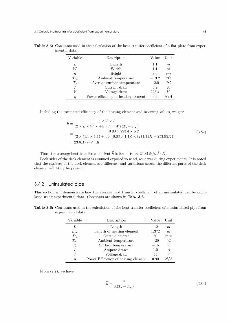
3.4 Calculating heat transfer coefficient from experimental data 43
Table 3.5: Constants used in the calculation of the heat transfer coefficient of a flat plate from exper-imental data.
Variable Description Value UnitL Length 1.1 mW Width 1.1 mh Height 3.0 cm
T∞ Ambient temperature −19.2 CTs Average surface temperature −2.0 CI Current draw 5.2 AV Voltage draw 223.4 Vη Power efficiency of heating element 0.90 N/A
Including the estimated efficiency of the heating element and inserting values, we get:
h = η × V × I
(2 × L × W × +4 × h × W ) (Ts − T∞)
= 0.90 × 223.4 × 5.2(2 × (1.1 × 1.1) + 4 × (0.03 × 1.1)) × (271.15K − 253.95K)
= 23.81W/m2 · K
(3.82)
Thus, the average heat transfer coefficient h is found to be 23.81W/m2 · K.Both sides of the deck element is assumed exposed to wind, as it was during experiments. It is noted
that the surfaces of the deck element are different, and variations across the different parts of the deckelement will likely be present.
3.4.2 Uninsulated pipeThis section will demonstrate how the average heat transfer coefficient of an uninsulated can be calcu-lated using experimental data. Constants are shown in Tab. 3.6.
Table 3.6: Constants used in the calculation of the heat transfer coefficient of a uninsulated pipe fromexperimental data.
Variable Description Value UnitL Length 1.2 m
Lhe Length of heating element 1.372 mDo Outer diameter 50 mmT∞ Ambient temperature −20 CTs Surface temperature −15 CI Ampere drawn 1.0 AV Voltage draw 55 Vη Power Efficiency of heating element 0.90 N/A
From (2.7), we have:
h = q
A(Ts − T∞)(3.83)

44 3 Calculations
As the heating element is 1.372 m long, the heat transfer rate per meter needs to be calculated:
q′ = q
L
= ηV I
Lhe
= 0.9 × 55 × 1.01.372
= 36.07W/m
(3.84)
Including the estimated efficiency of the heating element and inserting values, we get:
h = q′ × L
(L × (2πro)) × (Ts − T∞)
= 36.07 × 1.2(1.2 × (2π × 0.025)) × (258.15 − 253.15)
= 45.92W/m2 · K
(3.85)
Thus, the average heat transfer coefficient h is found to be 45.92W/m2 · K.
3.4.3 Insulated pipeThis section will demonstrate how the average heat transfer coefficient of an insulated pipe can becalculated using experimental data. Constants are shown in Tab. 3.6.
Table 3.7: Constants used in the calculation of the heat transfer coefficient of a insulated pipe fromexperimental data.
Variable Description Value UnitL Length 1.04 mD Diameter 50 mm
Lhe Length of heating element 1.372 mkins Thermal conductivity of insulation 3.30 × 10⁻² W/m · Ktins Thickness of insulation 10 mmT∞,2 Ambient temperature −20 CTs, 1 Surface temperature of pipe 45.35 C
I Ampere drawn 1.0 AV Voltage draw 56.2 Vη Power Efficiency of heating element 0.90 N/A
Equation (2.7) can be adopted to represent the overall heat transfer coefficient, U :
U = q
A(Ts − T∞)(3.86)
As the heating element is 1.372 m long, the heat transfer rate per meter needs to be calculated:
q′ = q
L
= ηV I
Lhe
= 0.9 × 56.2 × 1.01.372
= 36.86W/m
(3.87)

3.4 Calculating heat transfer coefficient from experimental data 45
Including the estimated efficiency of the heating element and inserting values, we get:
U = q′ × L
(L × (2πro)) × (Ts − T∞)
= 36.86 × 1.04(×(1.04 × (2π × 0.035)) × (318.5 − 253.15)
= 2.56W/m2 · K
(3.88)
Thus, the average overall heat transfer coefficient U is found to be 2.56W/m2 · K.

46

CHAPTER 4Experiments
The experiments were designed, planned and performed as a joint project with Jino Peechanatt.
4.1 Equipment configuration
4.1.1 PipesThe configuration used for measuring the average heat transfer coefficient is inspired by the work ofManohar and Ramroop (2010). However, the final configuration used is different, as the effect ofstaggered flow with multiple pipes of different diameters is also of interest and the testing jig neededto be portable in order to perform field experiments. The testing rig was constructed using perforatedangle iron, and bolted into shape. Triangular corner pieces were used to create additional stability, andthe entire jig was bolted into place on a pallet to enable easy transportation. A picture of the testingrig is found in Fig. 4.1.
Figure 4.1: Picture of the testing rig mounted on a pallet ©Bjarte Odin Kvamme.
The dimensions of the rig are: 111 cm x 66 cm x 92 cm (L x W x H). The height of the pipes isadjustable to allow for an optimal position both in the climate laboratory and aboard KV Svalbard.Pipe clamps with rubber padding were used to hold the steel pipes in place. These mounts are heightadjustable, to be able to test for different types and combinations of staggered flow. The method usedfor mounting the pipes are identical to what would be used in the industry, and will work as a heattransfer bridge. The steel pipes were cut to a length of 120 cm, and had a wall thickness of 2 mm.

48 4 Experiments
36 86 10 80 1040 80 10 86 36
All dimensions in mm
1200
1372
300 300 300 300
Sensor 1, 2 Sensor 3, 4 Sensor 5, 6
Figure 4.2: Sketch of insulated pipe as tested.
The steel quality used was DIN 2394. The pipes were insulated with Armaflex® AF-1, 10 mm thickinsulation to better simulate real-life industry use, and to provide a smooth surface, avoiding localturbulence over the areas where the sensors were mounted. Details about the insulation can be foundin Armacell Norway (2016). The insulation has a rated thermal conductivity of 0.033W/m · K. Adrawing of the 50 mm insulated pipe with dimensions is found in Fig. 4.2. For the 25 mm pipe, allmeasurements are the same, apart from the diameter. It should be noted that the uninsulated sectionshad a significant impact on the heat loss, and for future experiments, the entire pipe should either beinsulated or uninsulated. This is discussed further in Chapter 6.1. The end caps for the pipes weredesigned in OpenSCAD and printed in extruded ABS plastic using the 3D printing laboratory at theUniversity of Stavanger.
Heating elements are used to create a constant heat flux from the pipes. The heating elements weresecured to the end caps using fire retardant silicone sealant. The heating elements were obtained fromRS Components, and have a nominal output of 1000 W at 240 V AC. As this heat flux is much higherthan expected real-life applications, the output of the heating elements was controlled using a variac.A variac is a variable transformer which regulates the output voltage. As the resistance of each heatingelement is constant, the power output from the heating elements is proportional to the voltage applied.The resistances for each element were measured, and are presented in Tab. 4.1.
Table 4.1: Resistances of heating elements.
Diameter Pipe # Resistance (Ω)25 mm 1 57.125 mm 2 58.925 mm 3 57.650 mm 4 58.250 mm 5 57.650 mm 6 58.6
Based on the measured resistances, the total resistance can be calculated for any combination of theelements above using Ohm’s Law of resistance for parallel loads (2.13).
4.1.2 Deck elementThe deck element used was provided by GMC Maritime AS, and has a rated maximum effect of 1400W/m2 at 230 V AC. The deck element is created by using a mixture of epoxy with aluminium fragmentswith quartz sand of different sizes in the top layer to generate the required friction. The aluminiumfragments are used to distribute the heat quicker throughout the deck element. In Fig. 4.3 a picture

4.1 Equipment configuration 49
of the deck element is shown. The black tape marks out two squares, the outermost is 1.0 m x 1.0 mand the innermost is 0.7 m x 0.7 m. The silver tape was used to keep the tape in place when subjectedto wind. A description of key components is found in Tab. 4.2.
Figure 4.3: Deck element positioned for testing.
Table 4.2: Key components of tested deck element as shown in Fig. 4.3.
Number Description1 GMC’s temperature and humidity sensor2 Air temperature thermocouple3 Wind sensor4 Deck element with installed heat tracing
4.1.3 Data loggerThe data logger used in the experiment is an Arduino Uno R3. The code used in the data logging isfound in Appendix A.
The temperature sensors used for measuring the temperature of the pipe are Maxim IntegratedDS18B20. This temperature sensor has a rated accuracy of ±0.5 C for temperatures between −10 C

50 4 Experiments
and +85 C, and an overall range from −55 C and +125 C. The resolution is configured to be 0.0625 C.Further information about the DS18B20 can be found in Maxim Integrated (2010).
Ideally, sensors with higher accuracy should have been used, preferably thermocouples or thermis-tors. A total of 18 sensors was required to perform temperature measurements at all three pipessimultaneously. The cost procuring 18 thermocouple amplifiers (or datalogger(s) capable of this num-ber of thermocouples) would have increased the cost to a point way above the budget of this thesis, andwas thus discarded.
For measuring the ambient temperature and humidity, a DHT22 digital temperature and humiditysensor was used. Further information about the DHT22 sensor can found in Aosong Electronics Co.(2010).
A picture of the Arduino during testing is found in Fig. 4.5. A picture of the breakout board usedfor connecting sensors is found in Fig. 4.4. Key components are marked, with descriptions presentedin Tab. 4.3.
Figure 4.4: Breakout board used for connecting sensors ©Bjarte Odin Kvamme.
Table 4.3: Description of key components on breakout board as shown in Fig. 4.4.
Number Description1 Connectors for temperature sensor cables2 Connector for DHT22 temperature and humidity sensor3 Connector for wind sensor4 Voltage divider from 10 V to 4 V5 Connectors going to data logger
The temperature sensors and the humidity sensor were calibrated to GMC Maritime’s temperatureand humidity sensor. The room temperature was set to -20 C and was left to stabilize for four hours.

4.1 Equipment configuration 51
Figure 4.5: Arduino based data logger, configured for testing ©Bjarte Odin Kvamme.
The measured temperatures were averaged out, and the offset to the GMC Maritime’s temperaturesensor was found. A table of the offsets applied to the measurements are found in Tab. 4.4.

52 4 Experiments
Table 4.4: Calibrated offset of temperature and humidity sensors.
Name Serial number Measured OffsetAmbientT DHT22 Temperature -18.98 -1.02AmbientH DHT22 Humidity 52.52 3.48
Sensor 1 28FFACC2641503AE -20.34 0.34Sensor 2 28FF5FEA64150196 -19.95 -0.05Sensor 3 28FF8FE8641501CF -20.31 0.31Sensor 4 28FF1CC564150367 -20.44 0.44Sensor 5 28FF1EAF64150231 -20.23 0.23Sensor 6 28FFECA864150292 -20.32 0.32Sensor 7 28FFC5AD64150346 -20.09 0.09Sensor 8 28FFB8AE64150211 -20.17 0.17Sensor 9 28FFD74863150255 -20.25 0.25
Sensor 10 28FFB2CB641502BD -20.37 0.37Sensor 11 28FFDBCA641502D0 -20.09 0.09Sensor 12 28FFB8AE64150211 -20.17 0.17Sensor 13 28818A22050000F7 -19.30 -0.70Sensor 14 28FFD5A164150328 -20.20 0.20Sensor 15 28FFD3E764150203 -20.12 0.12Sensor 16 28FFE0C3641503E9 -20.26 0.26Sensor 17 28FF42BE6415036C -20.23 0.23Sensor 18 28FFECAA641503CB -20.28 0.28
4.2 Laboratory experiments
The laboratory experiments were performed at GMC Maritime’s climate laboratory at Buøy. Theclimate laboratory offers great control and remote access functionality, which made it significantlyeasier for us to perform our experiments. A screenshot of the control panel for the control system isfound in Fig. 4.6. A total of 387 hours and 30 minutes of experiments have been performed, consumingapproximately 14 000 kWh of electricity.
Fig. 4.7 shows the test rig as installed in the climate laboratory, rigged up for Experiment 1. Fig.4.8 shows an overhead view of the rig. A description of the key components is found in Tab. 4.5.
Table 4.5: Key components of testing rig.
Number Description1 GMC’s temperature and humidity sensor2 DHT22 temperature and ambient sensor3 Breakout board for sensor connections4 Heating element protrusion and power connection5 Approximate location of sensor 5 & 66 Wind speed sensor7 Cable connection to the variac8 Approximate location of sensor 3 & 49 Approximate location of sensor 1 & 2
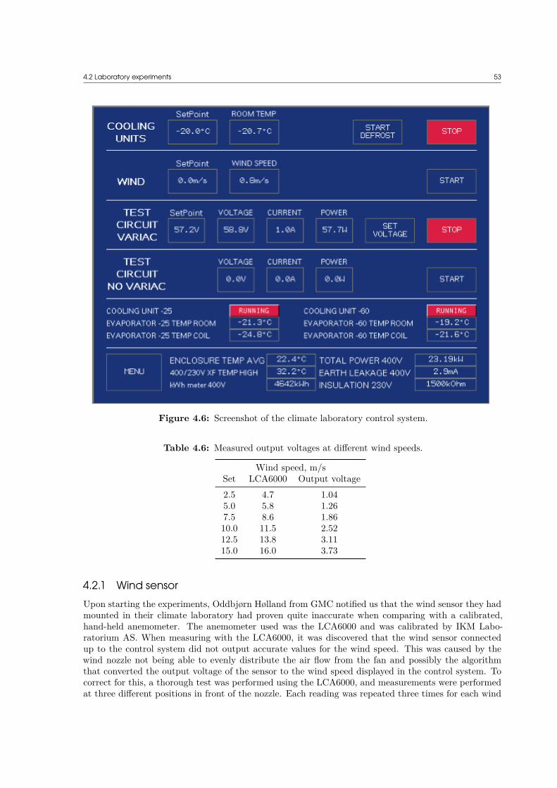
4.2 Laboratory experiments 53
Figure 4.6: Screenshot of the climate laboratory control system.
Table 4.6: Measured output voltages at different wind speeds.
Wind speed, m/sSet LCA6000 Output voltage2.5 4.7 1.045.0 5.8 1.267.5 8.6 1.8610.0 11.5 2.5212.5 13.8 3.1115.0 16.0 3.73
4.2.1 Wind sensorUpon starting the experiments, Oddbjørn Hølland from GMC notified us that the wind sensor they hadmounted in their climate laboratory had proven quite inaccurate when comparing with a calibrated,hand-held anemometer. The anemometer used was the LCA6000 and was calibrated by IKM Labo-ratorium AS. When measuring with the LCA6000, it was discovered that the wind sensor connectedup to the control system did not output accurate values for the wind speed. This was caused by thewind nozzle not being able to evenly distribute the air flow from the fan and possibly the algorithmthat converted the output voltage of the sensor to the wind speed displayed in the control system. Tocorrect for this, a thorough test was performed using the LCA6000, and measurements were performedat three different positions in front of the nozzle. Each reading was repeated three times for each wind

54 4 Experiments
Figure 4.7: Picture of the test rig as installed in GMC’s climate laboratory ©Bjarte Odin Kvamme.
Figure 4.8: Overhead view of the test rig, with key components marked ©Bjarte Odin Kvamme.
speed, and written down. The findings are presented in Tab. 4.7. A diagram of the wind nozzle withthe dimensions and the measurement locations are presented in Fig. 4.10. Before connecting the windsensor to the Arduino for use in the field experiments, we also performed testing of the output voltageto be able to establish the curve. The measured output voltages at various wind speeds are presentedin Tab. 4.6 and a plot of the curve is presented in Fig. 4.9, where the curve was fitted in MicrosoftExcel. The gradient of the trend line was used in the Arduino code to calculate the wind speed given avoltage. This approximation proved accurate for the wind speed range for these experiments, but couldbe further improved by acquiring more data.

4.2 Laboratory experiments 55
y = 4.2806x + 0.4572
0
2
4
6
8
10
12
14
16
18
0.5 1.0 1.5 2.0 2.5 3.0 3.5 4.0
Win
d s
pe
ed
, m
/s
Sensor output voltage, V
Wind speed / voltage
Wind speed Linear (Wind speed)
Figure 4.9: Plot of wind speed / voltage from Tab. 4.6.
Table 4.7: Corrected wind speed measurements.
Wind speed, m/sGMC LCA6000
Set Reported Pos. 1 Pos. 2 Pos. 3 Avg.2.5 3.5 4.6 5.3 4.9 4.905.0 5.0 6.1 7.1 6.7 6.637.5 7.5 9.0 10.3 9.6 9.6310.0 10.1 11.4 13.6 13.0 12.6712.5 12.5 13.6 16.0 14.5 14.7015.0 15.0 17.9 18.6 16.4 17.63

56 4 Experiments
Figure 4.10: Diagram of the wind nozzle with dimensions and measurement location.

4.3 Testing methodology 57
4.3 Testing methodology
4.3.1 PipesThe testing was performed using different configurations of the pipes and deck elements. The variousconfigurations are shown in Tab. 4.8. Throughout the testing of the pipes, the temperature was keptat −20 C. Each experiment was performed at four different wind speeds: 0, 5, 10 and 15 m/s, andrepeated three times to confirm the findings.
Additional experiments were initially planned, but the insulation applied on the pipes significantlyincreased the time required for the pipes to stabilize, and fewer experiments had to be performed inorder to fit the time-frame allocated. Before the insulation was applied, it took ∼ 30 minutes to stabilize,compared to ∼ 120 minutes after.
Table 4.8: Experiments performed.
Experiment # Pipe 1, 2, 3 Description1 O x x 1 x 50 mm pipe2 O x O 2 x 50 mm pipes with gap3 O O O 3 x 50 mm pipes4 O x x 1 x 50 mm pipe, with ice glazing5 O x x 1 x 50 mm pipe, with ice coating6 O x x 1 x 50 mm pipe, with rough surface7 o x O 1 x 25 mm pipe and 1x 50 mm pipe8 o x x 1 x 25 mm pipe9 o x o 2 x 25 mm pipes with gap10 O x o 1 x 50 mm pipes and 1x 25 mm pipe11 O x x 1 x 50 mm pipe without insulation12 Plate Deck element, rough surface
o = 25 mm, O = 50 mm, x = empty
The temperature readings from the temperature sensors were monitored in real-time using theserial output on the Arduino to a CSV file on a computer. This CSV file was connected to MicrosoftExcel, where the data was automatically refreshed every minute to show key numbers and plots of thetemperature readings. This spreadsheet was used to identify when all sensors had stabilized, that is,showed a temperature difference of less than 0.5 C over a period of 10 minutes between the maximumand minimum value obtained in this period. After the sensors had stabilized, the test was concluded,and we proceeded to the next test.
The following testing procedure was utilized when rigging up for the experiments:
1. Position the testing rig in the cooling room, directly in front of the wind tunnel. Adjust the heightso that the pipes are in the middle of the air flow.
2. Connect up the wind speed sensor to the grey junction box on the testing jig.
3. Position the ambient temperature sensor and connect it up to the grey junction box.
4. Select pipes according to schedule.
5. Position the temperature sensors along the lines of the black markings on the pipe. One temper-ature sensor at the top, and another at the bottom of the pipe. Secure the temperature sensor tothe pipe with aluminium tape.
6. Connect the temperature sensors to the grey junction box.
7. Connect the power cables to the heating elements.

58 4 Experiments
8. Connect a multimeter in series with one of the leads connecting to the variac, and set it to measurethe current.
9. Connect a multimeter in parallel with the two leads connecting to the variac, and set it to measurethe voltage.
10. Connect the data cable from the grey junction box to the Arduino.
11. Connect power to the Arduino.
12. Verify that the logging has started. The LEDs work like a heartbeat sensor and will rapidly flashgreen when logging has started.
13. Close the doors to the cooling room, and allow the temperature to settle down to -20 C.
14. Adjust the output voltage of the variac until the measured current is equal to 1 A per pipeconnected. This equals ∼50W with a resistance of 58.5 Ω.
Between each run, the following procedure was followed:
1. Confirm that the temperature logger is working, and logging the data
2. Cool the room down to -20 C, set the wind to 7.5 m/s to cool down the pipes faster
3. Once the pipes have stabilized at -20 C, write down the time of start, activate the heating elementinside, and wait for the pipe to stabilize at the higher temperature.
4. Once the pipe has stabilized at higher temperature, write down the time in the experiment log,turn on the fan, and set it to 5 m/s wind speed
5. Wait for the temperature to settle again, write down the time in the experiment log and increasethe wind speed to 10 m/s
6. Wait for the temperature to settle again, write down the time in the experiment log and increasethe wind speed to 15 m/s.
7. After the temperature has stabilized again, write down the time in the experiment log, turn offthe heating element, and set the wind to 7.5 m/s to cool down the pipe to -20 C for the next run.
A time series plot of Experiment 4 is plotted in Fig. 4.11. The different wind speeds are clearlyvisible as drops in temperature. The added heat from the fan is also visible in the ambient temperature,and the ambient temperature increases slightly when the fan speed was set to 10 m/s and 15 m/s. Thedrop in ambient temperature is caused by stopping the fan, thus removing the added heat from theelectric motor in the fan.

4.3Testing
methodology
59
-30
-20
-10
0
10
20
30
40
50
60
11/0
4/2
016
10
:11
11/0
4/2
016
11
:00
11/0
4/2
016
11
:48
11/0
4/2
016
12
:36
11/0
4/2
016
13
:24
11/0
4/2
016
14
:12
11/0
4/2
016
15
:01
11/0
4/2
016
15
:49
11/0
4/2
016
16
:37
11/0
4/2
016
17
:25
11/0
4/2
016
18
:14
11/0
4/2
016
19
:02
11/0
4/2
016
19
:50
11/0
4/2
016
20
:38
11/0
4/2
016
21
:26
11/0
4/2
016
22
:15
11/0
4/2
016
23
:03
11/0
4/2
016
23
:51
12/0
4/2
016
00
:39
12/0
4/2
016
01
:28
12/0
4/2
016
02
:16
12/0
4/2
016
03
:04
12/0
4/2
016
03
:52
12/0
4/2
016
04
:40
12/0
4/2
016
05
:29
12/0
4/2
016
06
:17
12/0
4/2
016
07
:05
12/0
4/2
016
07
:53
12/0
4/2
016
08
:41
12/0
4/2
016
09
:30
12/0
4/2
016
10
:18
12/0
4/2
016
11
:06
12/0
4/2
016
11
:54
12/0
4/2
016
12
:43
12/0
4/2
016
13
:31
12/0
4/2
016
14
:19
12/0
4/2
016
15
:07
12/0
4/2
016
15
:55
12/0
4/2
016
16
:44
12/0
4/2
016
17
:32
12/0
4/2
016
18
:20
12/0
4/2
016
19
:08
12/0
4/2
016
19
:56
12/0
4/2
016
20
:45
12/0
4/2
016
21
:33
12/0
4/2
016
22
:21
12/0
4/2
016
23
:09
12/0
4/2
016
23
:58
13/0
4/2
016
00
:46
13/0
4/2
016
01
:34
13/0
4/2
016
02
:22
13/0
4/2
016
03
:10
13/0
4/2
016
03
:59
13/0
4/2
016
04
:47
13/0
4/2
016
05
:35
Time series plot of Experiment 4
AmbientT Sec. 1 - Top Sec. 1 - Bottom Sec. 2 - Top Sec. 2 - Bottom Sec. 3 - Top Sec. 3 - Bottom
Figure 4.11: Time series plot of Experiment 4.

60 4 Experiments
4.3.2 Deck elementOur data logger could not be used for testing the deck element. This was due to the temperaturesensors used in the deck element were thermocouples, and required amplifiers before data could be readfrom them. The deck element was brand new, and the thermocouples installed did not have terminalsattached so they couldn’t be connected to GMC’s system. One thermocouple was mounted at the outletof wind nozzle to get an accurate reading of the temperature of the air flowing over the deck element.For measuring the surface temperatures, a FLIR A315 thermal imaging camera was used to measurethe maximum, minimum and average surface temperatures across the 0.7 m x 0.7 m section of the deckelement. Further information about the FLIR A315 can be found in FLIR Systems, Inc. (2016). Thedeck element was tested under different temperature and wind conditions to test the required practicein both the Polar Code (IMO, 2016) and DNV GLs Operational Standard for Winterization in coldclimate operations (DNV GL, 2015). The tests were performed at −15 C, −20 C, −30 C and −35 C.At each temperature, the deck element was subjected to wind speeds of 0, 5, 10 and 15 m/s, andrepeated three times to confirm the findings.
As the deck element was self-regulating, the current draw, voltage and calculated power was recordedfrom GMC’s control system at the end of each test to be able to calculate the heat transfer coefficient.
Initially, each test was run for one hour, but we found that the temperature of the deck element wasnot able to stabilize properly. We increased the duration of each test to counteract this, but the powerusage of the deck element was significantly higher than expected even when no wind was flowing overthe deck element.
4.4 Field experimentsThe field experiments performed in the thesis were performed as a part of SARex. SARex is a researchproject arranged by GMC Maritime AS and the University of Stavanger in cooperation with the Nor-wegian Coast Guard. The fieldwork was performed on the Norwegian Coast Guard vessel KV Svalbardin Woodfjorden, North Spitzbergen. The following entities participated in the field work:
• University of Stavanger (UiS)
• GMC Maritime AS
• The Norwegian Coast Guard
• UiT The Arctic University of Norway
• St. Olav’s Hospital in Trondheim
• Norwegian Armed Forces
• Eni Norge AS
• American Bureau of Shipping (ABS)
• Norwegian University of Science and Technology (NTNU) in Trondheim
• North University in Bodø
• Norwegian Maritime Authority (NMA)
• Petroleum Safety Authority Norway (PSA)
• Viking life-saving equipment
• Norsafe
The fieldwork took place 22 - 29 April 2016, and had the following objectives:

4.4 Field experiments 61
1. Investigate the adequacy of the rescue program required by the Polar code (IMO, 2016)
2. Study the effectiveness of launching, accessing and rescuing people from life boats and life raftswhen in cold and ice infested waters
3. Study the adequacy of standard lifeboats and life rafts for use in ice infested waters
4. Study the adequacy of standard survival equipment for use in ice infested waters
5. Study winterization means to improve the suitability of equipment to be used for rescue operationsin cold regions and ice infested waters
6. Train Norwegian Coast Guard personnel on emergency procedures in ice infested waters withparticular reference to evacuation and rescue from cruise ships
The field work undertaken as part of this thesis, falls under Objective 5. The purpose of the fieldexperiments is to get real-life conditions and scenarios in which the pipes are likely to be used. Inthe laboratory experiments, the pipe was subjected to a constant flow of air from a constant angle ofincident. This represents a worst case scenario, and does not represent realistic usage. The testing rigwas positioned on the aft deck of KV Svalbard with a wind sensor mounted, and the conditions weremonitored and logged with the temperature logger. An omnidirectional wind speed sensor was used,but the angle of incident of the wind was not recorded.
The following scenarios were tested:
• Uninsulated 50 mm pipe
• Insulated 50 mm pipe
More scenarios were planned, but were not performed due to technical difficulties. Both pipes weretested simultaneously. During the experiment, difficulties were encountered with the data logger. Thelogger stopped working after approximately one-two hours and had to be manually restarted. This isbelieved to be caused by the Arduino not functioning properly in cold temperatures. After the problemwas found, the data logger was moved inside a workshop and no problems were encountered since.
The experiments were performed from 25.04 2016 16:43 to 28.04 2016 13:51, ranging from latitudesof 7930N to 8030N, and longitudes of 940E to 1030E.

62

CHAPTER 5Results
The experiments were performed as a joint project with Jino Peechanatt. The results have been dividedup between us for further analysis. In this thesis, emphasis will be on different surface coatings ofsingle pipe configurations. Peechanatt (2016) looks into the effects of multiple pipes in a staggeredconfiguration, which was performed in Experiment 2, 3, 7, 9 and 10.
Instructions for obtaining the full experimental data files is found in Appendix E.In Tab. 5.1 a list of the different symbols and subscripts used in the tables are presented. Fig.
5.1 shows a sketch of the different zones used for calculating the heat transfer coefficient.
Table 5.1: Description of headers used in results.
SymbolsT Temperature, CU Overall heat transfer coefficient, W/m2 · K
Subscriptsavg Averaged over the entire pipetop Average of the three sensors on the top of the pipe
btm Average of the three sensors on the bottom of the pipesec, 1 Average of the two sensors in position 1 of the pipesec, 2 Average of the two sensors in position 2 of the pipesec, 3 Average of the two sensors in position 3 of the pipe
sec,1 sec,2 sec,3 top
bottom
Figure 5.1: Sketch of the different zones used for calculating the overall heat transfer coefficient.

64 5 Results
5.1 Experiment 1The configuration tested in this experiment was a single, insulated 50 mm pipe. The temperatures andthe overall heat transfer coefficient at different locations on the pipe is presented in Tab. 5.2. Plots ofthe overall heat transfer coefficient at different locations are presented in Fig. 5.2 & 5.3.
2.20
2.40
2.60
2.80
3.00
3.20
0 m/s 5 m/s 10 m/s 15 m/s
U (
W/m
² K
)
Experiment 1 - Overall heat transfer co-efficient
Top
Average
Bottom
Figure 5.2: Experiment 1: Overall heat transfer coefficient at different wind speeds.
2.20
2.40
2.60
2.80
3.00
3.20
3.40
Section 1 Section 2 Section 3
U (
W/m
² K
)
Experiment 1 - Overall heat transfer co-efficient, by section
0 m/s
5 m/s
10 m/s
15 m/s
Figure 5.3: Experiment 1: Overall heat transfer coefficient at different wind speeds, by section.
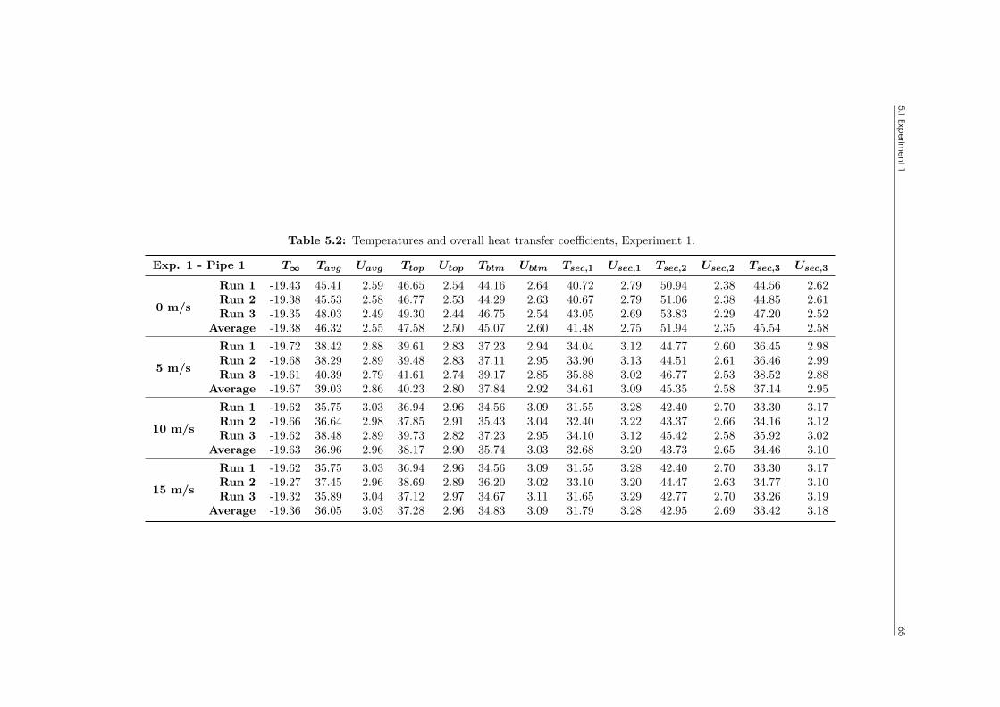
5.1Experim
ent165
Table 5.2: Temperatures and overall heat transfer coefficients, Experiment 1.
Exp. 1 - Pipe 1 T∞ Tavg Uavg Ttop Utop Tbtm Ubtm Tsec,1 Usec,1 Tsec,2 Usec,2 Tsec,3 Usec,3
0 m/s
Run 1 -19.43 45.41 2.59 46.65 2.54 44.16 2.64 40.72 2.79 50.94 2.38 44.56 2.62Run 2 -19.38 45.53 2.58 46.77 2.53 44.29 2.63 40.67 2.79 51.06 2.38 44.85 2.61Run 3 -19.35 48.03 2.49 49.30 2.44 46.75 2.54 43.05 2.69 53.83 2.29 47.20 2.52
Average -19.38 46.32 2.55 47.58 2.50 45.07 2.60 41.48 2.75 51.94 2.35 45.54 2.58
5 m/s
Run 1 -19.72 38.42 2.88 39.61 2.83 37.23 2.94 34.04 3.12 44.77 2.60 36.45 2.98Run 2 -19.68 38.29 2.89 39.48 2.83 37.11 2.95 33.90 3.13 44.51 2.61 36.46 2.99Run 3 -19.61 40.39 2.79 41.61 2.74 39.17 2.85 35.88 3.02 46.77 2.53 38.52 2.88
Average -19.67 39.03 2.86 40.23 2.80 37.84 2.92 34.61 3.09 45.35 2.58 37.14 2.95
10 m/s
Run 1 -19.62 35.75 3.03 36.94 2.96 34.56 3.09 31.55 3.28 42.40 2.70 33.30 3.17Run 2 -19.66 36.64 2.98 37.85 2.91 35.43 3.04 32.40 3.22 43.37 2.66 34.16 3.12Run 3 -19.62 38.48 2.89 39.73 2.82 37.23 2.95 34.10 3.12 45.42 2.58 35.92 3.02
Average -19.63 36.96 2.96 38.17 2.90 35.74 3.03 32.68 3.20 43.73 2.65 34.46 3.10
15 m/s
Run 1 -19.62 35.75 3.03 36.94 2.96 34.56 3.09 31.55 3.28 42.40 2.70 33.30 3.17Run 2 -19.27 37.45 2.96 38.69 2.89 36.20 3.02 33.10 3.20 44.47 2.63 34.77 3.10Run 3 -19.32 35.89 3.04 37.12 2.97 34.67 3.11 31.65 3.29 42.77 2.70 33.26 3.19
Average -19.36 36.05 3.03 37.28 2.96 34.83 3.09 31.79 3.28 42.95 2.69 33.42 3.18

66 5 Results
5.2 Experiment 4The configuration tested in this experiment was a single, insulated 50 mm pipe with ice glazing. Thetemperatures and the overall heat transfer coefficient at different locations on the pipe is presented inTab. 5.3. Plots of the overall heat transfer coefficient at different locations are presented in Fig. 5.4& 5.5.
2.20
2.40
2.60
2.80
3.00
3.20
0 m/s 5 m/s 10 m/s 15 m/s
U (
W/m
² K
)
Experiment 4 - Overall heat transfer co-efficient
Top
Average
Bottom
Figure 5.4: Experiment 4: Overall heat transfer coefficient at different wind speeds.
2.20
2.40
2.60
2.80
3.00
3.20
3.40
Section 1 Section 2 Section 3
U (
W/m
² K
)
Experiment 4 - Overall heat transfer co-efficient, by section
0 m/s
5 m/s
10 m/s
15 m/s
Figure 5.5: Experiment 4: Overall heat transfer coefficient at different wind speeds, by section.

5.2Experim
ent467
Table 5.3: Temperatures and overall heat transfer coefficients, Experiment 4.
Exp. 4 - Pipe 1 T∞ Tavg Uavg Ttop Utop Tbtm Ubtm Tsec,1 Usec,1 Tsec,2 Usec,2 Tsec,3 Usec,3
0 m/s
Run 1 -19.42 46.45 2.58 47.67 2.53 45.24 2.63 41.80 2.77 51.86 2.38 45.70 2.61Run 2 -19.42 47.33 2.54 48.59 2.50 46.08 2.59 42.52 2.74 52.90 2.35 46.58 2.57Run 3 -19.50 47.40 2.54 48.64 2.49 46.17 2.58 42.75 2.73 53.01 2.34 46.46 2.57
Average -19.45 47.06 2.55 48.30 2.51 45.83 2.60 42.36 2.75 52.59 2.36 46.25 2.58
5 m/s
Run 1 -19.78 39.47 2.86 40.69 2.81 38.24 2.93 35.20 3.09 45.77 2.59 37.43 2.97Run 2 -19.66 38.43 2.92 39.64 2.86 37.22 2.98 34.26 3.15 44.62 2.64 36.40 3.03Run 3 -19.62 39.65 2.86 40.88 2.81 38.43 2.92 35.41 3.08 46.00 2.59 37.55 2.97
Average -19.69 39.18 2.88 40.40 2.82 37.96 2.94 34.96 3.11 45.46 2.61 37.13 2.99
10 m/s
Run 1 -19.62 37.23 2.99 38.45 2.92 36.02 3.05 32.96 3.23 44.02 2.67 34.73 3.12Run 2 -19.61 36.53 3.02 37.73 2.96 35.33 3.09 32.29 3.27 43.24 2.70 34.06 3.16Run 3 -19.64 38.00 2.94 39.23 2.88 36.77 3.01 33.64 3.19 44.89 2.63 35.47 3.08
Average -19.62 37.25 2.98 38.47 2.92 36.04 3.05 32.96 3.23 44.05 2.67 34.76 3.12
15 m/s
Run 1 -18.67 37.55 3.02 38.78 2.95 36.33 3.09 33.25 3.27 44.50 2.69 34.91 3.17Run 2 -19.11 36.78 3.04 38.00 2.97 35.57 3.10 32.52 3.29 43.70 2.70 34.13 3.19Run 3 -19.25 37.73 2.98 38.96 2.92 36.49 3.05 33.36 3.23 44.79 2.65 35.02 3.13
Average -19.01 37.35 3.01 38.58 2.95 36.13 3.08 33.04 3.26 44.33 2.68 34.69 3.16

68 5 Results
5.3 Experiment 5The configuration tested in this experiment was a single, insulated 50 mm pipe with an ice coating. Thetemperatures and the overall heat transfer coefficient at different locations on the pipe is presented inTab. 5.4. Plots of the overall heat transfer coefficient at different locations are presented in Fig. 5.6& 5.7.
2.20
2.40
2.60
2.80
3.00
3.20
0 m/s 5 m/s 10 m/s 15 m/s
U (
W/m
² K
)
Experiment 5 - Overall heat transfer co-efficient
Top
Average
Bottom
Figure 5.6: Experiment 5: Overall heat transfer coefficient at different wind speeds.
2.20
2.40
2.60
2.80
3.00
3.20
3.40
Section 1 Section 2 Section 3
U (
W/m
² K
)
Experiment 5 - Overall heat transfer co-efficient, by section
0 m/s
5 m/s
10 m/s
15 m/s
Figure 5.7: Experiment 5: Overall heat transfer coefficient at different wind speeds, by section.

5.3Experim
ent569
Table 5.4: Temperatures and overall heat transfer coefficients, Experiment 5.
Exp. 5 - Pipe 1 T∞ Tavg Uavg Ttop Utop Tbtm Ubtm Tsec,1 Usec,1 Tsec,2 Usec,2 Tsec,3 Usec,3
0 m/s
Run 1 -20.32 45.68 2.58 46.86 2.53 44.49 2.62 40.91 2.78 51.09 2.38 45.03 2.60Run 2 N/A N/A N/A N/A N/A N/A N/A N/A N/A N/A N/A N/A N/ARun 3 N/A N/A N/A N/A N/A N/A N/A N/A N/A N/A N/A N/A N/A
Average -20.32 45.68 2.58 46.86 2.53 44.49 2.62 40.91 2.78 51.09 2.38 45.03 2.60
5 m/s
Run 1 -19.54 39.51 2.88 40.71 2.82 38.31 2.94 35.35 3.10 45.90 2.60 37.28 2.99Run 2 N/A N/A N/A N/A N/A N/A N/A N/A N/A N/A N/A N/A N/ARun 3 N/A N/A N/A N/A N/A N/A N/A N/A N/A N/A N/A N/A N/A
Average -19.54 39.51 2.88 40.71 2.82 38.31 2.94 35.35 3.10 45.90 2.60 37.28 2.99
10 m/s
Run 1 -19.54 36.51 3.03 37.69 2.97 35.33 3.10 32.23 3.28 43.26 2.71 34.04 3.17Run 2 N/A N/A N/A N/A N/A N/A N/A N/A N/A N/A N/A N/A N/ARun 3 N/A N/A N/A N/A N/A N/A N/A N/A N/A N/A N/A N/A N/A
Average -19.54 36.51 3.03 37.69 2.97 35.33 3.10 32.23 3.28 43.26 2.71 34.04 3.17
15 m/s
Run 1 -19.23 37.31 3.01 38.53 2.94 36.10 3.07 32.92 3.26 44.35 2.67 34.67 3.15Run 2 N/A N/A N/A N/A N/A N/A N/A N/A N/A N/A N/A N/A N/ARun 3 N/A N/A N/A N/A N/A N/A N/A N/A N/A N/A N/A N/A N/A
Average -19.23 37.31 3.01 38.53 2.94 36.10 3.07 32.92 3.26 44.35 2.67 34.67 3.15

70 5 Results
5.4 Experiment 6The configuration tested in this experiment was a single, insulated 50 mm pipe, with a roughenedsurface. The surface of the insulation was coated in a mixture of glue and quartz grains with a sizeof 0.7-1.2 mm. The temperatures and the overall heat transfer coefficient at different locations on thepipe is presented in Tab. 5.5. Plots of the overall heat transfer coefficient at different locations arepresented in Fig. 5.8 & 5.9.
2.20
2.40
2.60
2.80
3.00
3.20
0 m/s 5 m/s 10 m/s 15 m/s
U (
W/m
² K
)
Experiment 6 - Overall heat transfer co-efficient
Top
Average
Bottom
Figure 5.8: Experiment 6: Overall heat transfer coefficient at different wind speeds.
2.00
2.20
2.40
2.60
2.80
3.00
3.20
Section 1 Section 2 Section 3
U (
W/m
² K
)
Experiment 6 - Overall heat transfer co-efficient, by section
0 m/s
5 m/s
10 m/s
15 m/s
Figure 5.9: Experiment 6: Overall heat transfer coefficient at different wind speeds, by section.

5.4Experim
ent671
Table 5.5: Temperatures and overall heat transfer coefficients, Experiment 6.
Exp. 6 - Pipe 2 T∞ Tavg Uavg Ttop Utop Tbtm Ubtm Tsec,1 Usec,1 Tsec,2 Usec,2 Tsec,3 Usec,3
0 m/s
Run 1 -19.27 52.96 2.31 53.75 2.29 52.18 2.34 50.41 2.40 59.31 2.13 49.17 2.44Run 2 -19.42 50.68 2.38 51.42 2.36 49.93 2.41 47.99 2.48 56.96 2.19 47.07 2.51Run 3 -19.46 51.84 2.34 52.61 2.32 51.06 2.37 49.03 2.44 58.12 2.15 48.36 2.46
Average -19.38 51.83 2.35 52.60 2.32 51.06 2.37 49.14 2.44 58.13 2.15 48.20 2.47
5 m/s
Run 1 -19.51 43.97 2.63 44.78 2.60 43.15 2.67 40.08 2.80 51.11 2.37 40.71 2.77Run 2 -19.52 42.23 2.71 43.02 2.67 41.44 2.74 38.25 2.89 49.10 2.43 39.34 2.84Run 3 -19.61 43.94 2.63 44.74 2.60 43.14 2.66 39.91 2.81 51.13 2.36 40.78 2.77
Average -19.55 43.38 2.65 44.18 2.62 42.58 2.69 39.41 2.83 50.45 2.39 40.28 2.79
10 m/s
Run 1 -19.35 43.32 2.67 44.13 2.63 42.50 2.70 39.46 2.84 50.91 2.38 39.59 2.83Run 2 -18.65 42.05 2.75 42.84 2.72 41.27 2.79 38.16 2.94 49.32 2.46 38.69 2.91Run 3 -18.92 43.13 2.69 43.93 2.66 42.33 2.73 39.21 2.87 50.62 2.40 39.56 2.86
Average -18.97 42.83 2.70 43.63 2.67 42.03 2.74 38.94 2.88 50.28 2.41 39.28 2.87
15 m/s
Run 1 -18.18 43.41 2.71 44.23 2.68 42.59 2.75 39.53 2.89 50.97 2.42 39.73 2.88Run 2 -17.42 42.97 2.77 43.76 2.73 42.18 2.80 39.08 2.96 50.30 2.47 39.52 2.93Run 3 -18.67 42.55 2.73 43.35 2.69 41.75 2.76 38.54 2.92 50.10 2.43 39.02 2.90
Average -18.09 42.98 2.74 43.78 2.70 42.17 2.77 39.05 2.92 50.46 2.44 39.43 2.90

72 5 Results
5.5 Experiment 8The configuration tested in this experiment was a single, insulated 25 mm pipe. The temperatures andthe overall heat transfer coefficient at different locations on the pipe is presented in Tab. 5.6. Plots ofthe overall heat transfer coefficient at different locations are presented in Fig. 5.10 & 5.11.
2.20
2.30
2.40
2.50
2.60
2.70
2.80
2.90
0 m/s 5 m/s 10 m/s 15 m/s
U (
W/m
² K
)
Experiment 8 - Overall heat transfer co-efficient
Top
Average
Bottom
Figure 5.10: Experiment 8: Overall heat transfer coefficient at different wind speeds.
2.00
2.20
2.40
2.60
2.80
3.00
3.20
Section 1 Section 2 Section 3
U (
W/m
² K
)
Experiment 8 - Overall heat transfer co-efficient, by section
0 m/s
5 m/s
10 m/s
15 m/s
Figure 5.11: Experiment 8: Overall heat transfer coefficient at different wind speeds, by section.

5.5Experim
ent873
Table 5.6: Temperatures and overall heat transfer coefficients, Experiment 8.
Exp. 8 - Pipe 1 T∞ Tavg Uavg Ttop Utop Tbtm Ubtm Tsec,1 Usec,1 Tsec,2 Usec,2 Tsec,3 Usec,3
0 m/s
Run 1 -19.62 91.05 2.39 90.10 2.41 92.00 2.37 83.43 2.56 99.72 2.21 90.00 2.41Run 2 -19.70 92.65 2.35 91.72 2.37 93.58 2.33 84.42 2.54 101.50 2.18 92.04 2.36Run 3 -19.42 92.05 2.37 91.10 2.39 92.99 2.35 83.65 2.56 100.82 2.20 91.66 2.38
Average -19.58 91.92 2.37 90.98 2.39 92.86 2.35 83.83 2.55 100.68 2.20 91.24 2.38
5 m/s
Run 1 -19.52 78.26 2.70 77.37 2.73 79.16 2.68 69.96 2.95 87.13 2.48 77.70 2.72Run 2 -19.57 78.92 2.68 78.03 2.71 79.80 2.66 70.46 2.93 87.52 2.47 78.77 2.68Run 3 -19.54 79.01 2.68 78.10 2.70 79.92 2.65 70.35 2.94 87.73 2.46 78.93 2.68
Average -19.54 78.73 2.69 77.83 2.71 79.63 2.66 70.26 2.94 87.46 2.47 78.47 2.69
10 m/s
Run 1 -18.50 78.38 2.73 77.48 2.75 79.27 2.70 69.95 2.99 87.58 2.49 77.60 2.75Run 2 -18.99 77.22 2.74 76.30 2.77 78.14 2.72 68.40 3.02 86.51 2.50 76.73 2.76Run 3 -19.01 79.31 2.69 78.35 2.71 80.27 2.66 70.31 2.96 88.62 2.45 78.99 2.69
Average -18.83 78.30 2.72 77.38 2.74 79.22 2.69 69.56 2.99 87.57 2.48 77.77 2.73
15 m/s
Run 1 -18.57 78.39 2.72 77.49 2.75 79.30 2.70 69.40 3.00 87.95 2.48 77.83 2.74Run 2 -17.66 78.90 2.73 77.98 2.76 79.81 2.71 69.95 3.01 88.29 2.49 78.46 2.75Run 3 -17.84 77.63 2.77 76.71 2.79 78.55 2.74 68.67 3.05 87.09 2.52 77.14 2.78
Average -18.02 78.31 2.74 77.39 2.77 79.22 2.72 69.34 3.02 87.77 2.50 77.81 2.76

74 5 Results
5.6 Experiment 11The configuration tested in this experiment was a single, uninsulated 50 mm pipe. The temperaturesand the overall heat transfer coefficient at different locations on the pipe is presented in Tab. 5.7.Plots of the overall heat transfer coefficient at different locations are presented in Fig. 5.12 & 5.13.
0.00
50.00
100.00
150.00
200.00
0 m/s 5 m/s 10 m/s 15 m/s
U (
W/m
² K
)
Experiment 11 - Overall heat transfer co-efficient
Top
Average
Bottom
Figure 5.12: Experiment 11: Overall heat transfer coefficient at different wind speeds.
0.00
20.00
40.00
60.00
80.00
100.00
120.00
140.00
160.00
180.00
Section 1 Section 2 Section 3
U (
W/m
² K
)
Experiment 11 - Overall heat transfer co-efficient, by section
0 m/s
5 m/s
10 m/s
15 m/s
Figure 5.13: Experiment 11: Overall heat transfer coefficient at different wind speeds, by section.

5.6Experim
ent1175
Table 5.7: Temperatures and overall heat transfer coefficients, Experiment 11.
Exp. 11 - Pipe 2 T∞ Tavg Uavg Ttop Utop Tbtm Ubtm Tsec Usec,1 Tsec,2 Usec,2 Tsec,3 Usec,3
0 m/s
Run 1 -19.70 -6.00 17.13 -5.31 16.31 -6.69 18.03 -7.03 18.52 -5.50 16.53 -5.46 16.48Run 2 -19.36 -4.78 16.11 -4.10 15.39 -5.46 16.90 -5.88 17.41 -4.05 15.33 -4.42 15.72Run 3 -19.44 -4.87 16.11 -4.23 15.43 -5.52 16.86 -5.69 17.07 -4.18 15.38 -4.76 15.99
Average -19.50 -5.22 16.43 -4.55 15.70 -5.89 17.25 -6.20 17.64 -4.58 15.73 -4.88 16.06
5 m/s
Run 1 -19.52 -16.45 76.49 -16.25 71.89 -16.64 81.72 -16.01 66.97 -16.79 86.02 -16.54 78.97Run 2 -19.42 -16.79 89.28 -16.56 82.10 -17.02 97.83 -16.35 76.69 -17.10 101.42 -16.90 93.43Run 3 -19.31 -16.65 88.07 -16.42 81.14 -16.87 96.29 -16.20 75.45 -16.97 100.37 -16.77 92.20
Average -19.41 -16.63 84.20 -16.41 78.10 -16.84 91.34 -16.19 72.77 -16.95 95.39 -16.74 87.69
10 m/s
Run 1 -18.80 -17.24 150.58 -17.06 134.98 -17.42 170.27 -17.05 134.11 -17.34 160.53 -17.34 160.34Run 2 -18.91 -17.33 148.53 -17.14 132.76 -17.52 168.53 -17.11 130.35 -17.45 160.26 -17.44 159.05Run 3 -18.73 -17.08 142.79 -16.90 128.31 -17.27 160.95 -16.87 126.59 -17.20 153.13 -17.18 151.97
Average -18.81 -17.22 147.22 -17.04 131.96 -17.40 166.49 -17.01 130.28 -17.33 157.90 -17.32 157.03
15 m/s
Run 1 -17.33 -15.84 157.24 -15.69 143.11 -15.99 174.46 -15.77 149.84 -15.87 160.24 -15.88 162.21Run 2 -17.99 -16.58 167.21 -16.43 150.62 -16.74 187.92 -16.50 158.24 -16.61 170.87 -16.63 173.33Run 3 -18.04 -16.65 169.17 -16.49 151.90 -16.81 190.87 -16.58 160.41 -16.68 172.15 -16.70 175.73
Average -17.79 -16.36 164.37 -16.20 148.44 -16.51 184.13 -16.28 156.03 -16.38 167.58 -16.41 170.21

76 5 Results
5.7 Deck elementTables with measured temperatures and power consumption during testing of the deck element ispresented in Tab. 5.8 & 5.8. The three runs for each temperature were averaged out, and the overallheat transfer coefficient is plotted in Fig. 5.14, and the power consumption versus wind speed isplotted in Fig. 5.15. The overall heat transfer coefficient was calculated using (2.7). The inputs usedwere the ambient temperature, Tamb, the average surface temperature, Ts,avg and the total surface areaof the deck element.
0
20
40
60
80
100
120
0 m/s 5 m/s 10 m/s 15 m/s
U (
W/m
² K
)
Wind speed
Deck element
Overall heat transfer coefficent vs wind speed
-15 °C
-20 °C
-30 °C
-35 °C
Figure 5.14: Plot of overall heat transfer coefficient versus wind speed for the deck element.
800
900
1000
1100
1200
1300
1400
1500
0 m/s 5 m/s 10 m/s 15 m/s
Po
we
r c
on
sum
ptio
n (
W)
Wind speed
Deck element
Power consumption vs wind speed
-15 °C
-20 °C
-30 °C
-35 °C
Figure 5.15: Plot of power consumption versus wind speed for the deck element.

5.7D
eckelem
ent77
Table 5.8: Measurements from deck element at -15 C and -20 C.
T∞,set u∞ Duration(h:mm)
T∞ Tair Ts,min Ts,max Ts,avg A V W U ∆WR
un#
1 -15 0 1:07 -14.0 -11.2 11.5 17.2 15.1 4.5 221.2 997.0 12.10 0.0-15 5 1:15 -13.6 -12.6 -0.8 7.3 3.7 4.8 222.3 1077.0 21.99 80.0-15 10 0:30 -13.1 -11.9 -4.4 3.0 -0.6 5.0 221.7 1104.0 31.25 107.0-15 15 0:30 -12.5 -11.5 -6.1 0.7 -2.6 5.1 222.1 1135.0 40.35 138.0
Run
#2 -15 0 2:45 -13.8 -11.2 18.0 26.4 23.9 3.8 225.7 876.0 8.19 0.0
-15 5 1:21 -14.0 -12.7 -9.5 7.6 3.5 4.7 224.8 1073.0 21.57 197.0-15 10 1:05 -13.7 -12.7 -11.7 1.8 -1.6 5.0 223.9 1131.0 32.86 255.0-15 15 1:14 -13.7 -12.3 -7.7 -0.9 -4.1 5.1 224.5 1165.0 42.93 289.0
Run
#3 -15 0 1:46 -13.7 -11.5 16.5 23.0 20.9 4.1 225.7 935.0 9.54 0.0
-15 5 1:11 -14.0 -13.1 -0.5 8.0 3.9 4.8 224.7 1078.0 21.27 143.0-15 10 1:02 -13.6 -12.3 -5.7 1.9 -1.5 5.0 224.3 1135.0 32.97 200.0-15 15 1:00 -12.8 -11.5 -7.2 0.3 -2.8 5.1 224.9 1155.0 40.57 220.0
Run
#1 -20 0 2:52 -18.7 -16.8 16.5 24.3 21.9 4.1 224.9 937.0 8.14 0.0
-20 5 4:19 -19.2 -17.7 -6.8 1.7 -2.1 5.2 222.5 1174.0 24.27 237.0-20 10 2:28 -19.3 -17.6 -11.7 -4.2 -7.8 5.5 224.2 1231.0 37.88 294.0-20 15 2:24 -18.8 -17.5 -12.9 -6.3 -9.5 5.6 225.6 1264.0 48.19 327.0
Run
#2 -20 0 2:01 -18.9 -17.6 14.8 21.8 19.5 4.3 226.2 972.0 8.93 0.0
-20 5 3:22 -19.0 -17.8 -7.0 1.8 -2.0 5.2 223.1 1180.0 24.45 208.0-20 10 6:03 -18.9 -18.2 -11.1 -3.7 -7.0 5.5 223.6 1236.0 36.60 264.0-20 15 3:16 -19.0 -18.3 -13.3 -6.8 -9.9 5.6 226.3 1272.0 49.24 300.0
Run
#3 -20 0 3:16 -19.1 -17.2 17.2 25.0 22.4 4.1 225.8 933.0 7.93 0.0
-20 5 1:52 -19.4 -18.6 -7.2 2.1 -2.0 5.2 224.6 1172.0 23.80 239.0-20 10 1:06 -18.8 -18.3 -10.7 -3.5 -6.8 5.4 226.9 1230.0 36.24 297.0-20 15 2:14 -18.8 -17.1 -13.0 -6.6 -9.6 5.6 223.8 1255.0 48.06 322.0

785
Results
Table 5.9: Measurements from deck element at -30 C and -35 C.
T∞,set u∞ Duration(h:mm)
T∞ Tair Ts,min Ts,max Ts,avg A V W U ∆W
Run
#1 -30 0 2:02 -30.9 -29.6 4.5 12.9 9.7 4.7 225.1 1075.0 9.35 0.0
-30 5 2:50 -28.8 -27.1 -20.5 -10.3 -14.9 5.7 226.5 1292.0 32.90 217.0-30 10 1:03 -25.4 -24.1 -22.3 -13.8 -17.7 5.8 226.3 1325.0 60.45 250.0-30 15 1:03 -31.6 -29.8 -28.0 -19.7 -23.4 5.9 225.6 1361.0 58.89 286.0
Run
#2 -30 0 2:27 -31.0 -29.5 5.7 13.3 10.1 4.7 228.3 1079.0 9.26 0.0
-30 5 1:03 -27.2 -26.9 -18.5 -7.8 -12.3 5.0 227.6 1158.0 27.43 79.0-30 10 1:00 -29.8 -28.4 -24.0 -15.4 -19.2 5.8 227.2 1320.0 43.79 241.0-30 15 1:00 -26.0 -23.1 -23.4 -16.4 -19.6 6.0 227.3 1359.0 75.36 280.0
Run
#3 -30 0 1:01 -25.9 -21.9 1.2 12.5 8.7 4.6 227.6 1060.0 10.81 0.0
-30 5 0:58 -27.5 -25.7 -17.3 -7.4 -11.5 5.5 225.2 1244.0 27.39 184.0-30 10 1:05 -28.3 -27.4 -23.2 -14.1 -18.3 5.8 224.5 1317.0 46.40 257.0-30 15 1:00 -31.4 -28.7 -28.2 -20.2 -24.1 6.0 224.8 1366.0 66.17 306.0
Run
#1 -35 0 5:16 -32.8 -31.1 -4.5 8.2 3.7 4.8 227.3 1111.0 10.73 0.0
-35 5 2:01 -25.2 -22.6 -17.7 -8.1 -12.3 5.7 225.3 1296.0 35.51 185.0-35 10 1:45 -31.4 -28.9 -29.0 -20.6 -24.6 6.2 225.7 1398.0 72.50 287.0-35 15 1:18 -28.2 -25.8 -26.9 -20.2 -23.1 6.2 226.0 1418.0 98.25 307.0
Run
#2 -35 0 2:17 -27.1 -23.9 -3.1 7.8 3.5 5.0 226.4 1138.0 13.10 0.0
-35 5 1:15 -29.5 -28.9 -18.6 -8.6 -12.9 5.7 226.0 1287.0 27.36 149.0-35 10 1:45 -29.7 -27.8 -26.9 -18.8 -22.5 6.1 226.0 1400.0 68.57 262.0-35 15 2:25 -25.6 -22.0 -25.2 -17.2 -21.6 6.2 225.6 1400.0 123.43 262.0
Run
#3 -35 0 2:57 -23.4 -19.7 -0.6 10.3 6.2 4.9 227.2 1122.0 13.39 0.0
-35 5 N/A N/A N/A N/A N/A N/A N/A N/A N/A N/A N/A-35 10 N/A N/A N/A N/A N/A N/A N/A N/A N/A N/A N/A-35 15 N/A N/A N/A N/A N/A N/A N/A N/A N/A N/A N/A

5.8 Theoretical calculations 79
5.8 Theoretical calculationsTo perform the theoretical calculations, the temperatures, power usage and pipe dimensions from Ex-periment 1 and 8 was used. Temperatures and wind speeds from Section 2 are selected for comparison,as the other gave insulation temperatures below the ambient temperatures, making the film tempera-ture inaccurate. Average heat transfer coefficients were calculated using the heat transfer correlationspresented in Chapter 2.2.2.
5.8.1 Experiment 1Theoretical results is presented in Tab. 5.10. A plot of the average overall heat transfer coefficientsacross the pipe is presented in Fig. 5.16. A plot of the overall heat transfer coefficient at Section 2 ispresented in Fig. 5.17.
2.50
2.55
2.60
2.65
2.70
2.75
2.80
6.63 m/s 12.67 m/s 17.63 m/s
U (
W/m
² K
)
Average overall heat transfer coefficient
Theoretical calculations, Experiment 1
Hilpert Original
Hilpert Updated
Fand & Keswani
Morgan
Whitaker
Churchill-Bernstein
Figure 5.16: Experiment 1: Theoretical overall heat transfer coefficients at different wind speeds.

80 5 Results
2.50
2.55
2.60
2.65
2.70
2.75
2.80
7.1 m/s 13.6 m/s 18.6 m/s
U (
W/m
² K
)
Average overall heat transfer coefficient
Theoretical calculations, Experiment 1, Section 2
Hilpert Original
Hilpert Updated
Fand & Keswani
Morgan
Whitaker
Churchill-Bernstein
Figure 5.17: Experiment 1: Theoretical overall heat transfer coefficients at different wind speeds atSection 2.

5.8Theoreticalcalculations
81
Table 5.10: Nusselt number, average and overall heat transfer coefficients, theoretical, based on Experiment 1.
Overall Section 1 Section 2 Section 3Correlation Nu hD U Nu hD U Nu hD U Nu hD U
6.63 m/s
Hilpert Original 109.17 34.78 2.59 104.00 33.13 2.58 115.35 36.75 2.60 110.09 35.07 2.59Hilpert Updated 123.33 39.29 2.62 115.36 36.75 2.60 130.32 41.51 2.63 124.37 39.62 2.62Fand & Keswani 302.35 96.32 2.72 101.18 32.23 2.58 321.53 102.43 2.73 305.21 97.23 2.72
Morgan 109.18 34.78 2.59 103.58 33.00 2.58 114.02 36.32 2.60 109.91 35.02 2.59Žukauskas 133.78 42.62 2.63 127.25 40.54 2.62 139.39 44.41 2.64 134.62 42.89 2.63Whitaker 150.12 47.82 2.65 143.69 45.77 2.64 155.31 49.48 2.65 151.25 48.18 2.65
Churchill-Bernstein 121.15 38.60 2.61 115.15 36.68 2.60 126.36 40.26 2.62 121.94 38.85 2.61
12.67 m/s
Hilpert Original 183.87 58.57 2.67 168.88 53.80 2.66 194.66 62.01 2.68 187.71 59.80 2.68Hilpert Updated 207.72 66.17 2.69 190.78 60.78 2.68 219.90 70.06 2.69 212.06 67.56 2.69Fand & Keswani 540.85 172.30 2.76 491.91 156.71 2.75 576.37 183.62 2.76 553.49 176.33 2.76
Morgan 177.06 56.41 2.67 162.48 51.76 2.66 187.57 59.76 2.68 180.81 57.60 2.67Žukauskas 197.30 62.86 2.68 185.19 59.00 2.68 205.87 65.58 2.69 200.37 63.83 2.68Whitaker 217.28 69.22 2.69 205.25 65.39 2.69 225.16 71.73 2.70 220.83 70.35 2.69
Churchill-Bernstein 182.42 58.11 2.67 170.33 54.26 2.66 191.08 60.87 2.68 185.51 59.10 2.68
17.63 m/s
Hilpert Original 239.88 76.42 2.70 242.84 77.36 2.70 250.45 79.79 2.71 226.32 72.10 2.70Hilpert Updated 271.00 86.33 2.71 274.34 87.40 2.72 282.94 90.14 2.72 255.67 81.45 2.71Fand & Keswani 727.65 231.81 2.77 737.65 234.99 2.77 763.50 243.23 2.77 681.89 217.23 2.77
Morgan 231.70 73.81 2.70 234.58 74.73 2.70 242.02 77.10 2.70 218.45 69.59 2.69Žukauskas 240.56 76.64 2.70 242.76 77.34 2.70 248.42 79.14 2.71 230.34 73.38 2.70Whitaker 262.66 83.68 2.71 265.92 84.71 2.71 269.55 85.87 2.71 252.34 80.39 2.71
Churchill-Bernstein 227.15 72.36 2.70 229.49 73.11 2.70 235.54 75.04 2.70 216.36 68.93 2.69

82 5 Results
5.8.2 Experiment 8Theoretical results is presented in Tab. 5.11. A plot of the average overall heat transfer coefficientsacross the pipe is presented in Fig. 5.18. A plot of the overall heat transfer coefficient at Section 2 ispresented in Fig. 5.19.
2.25
2.30
2.35
2.40
2.45
2.50
6.63 m/s 12.67 m/s 17.63 m/s
U (
W/m
² K
)
Average overall heat transfer coefficient
Theoretical calculations, Experiment 8
Hilpert Original
Hilpert Updated
Fand & Keswani
Morgan
Whitaker
Churchill-Bernstein
Figure 5.18: Experiment 8: Theoretical overall heat transfer coefficients at different wind speeds.
2.25
2.30
2.35
2.40
2.45
2.50
7.1 m/s 13.6 m/s 18.6 m/s
U (
W/m
² K
)
Average overall heat transfer coefficient
Theoretical calculations, Experiment 8, Section 2
Hilpert Original
Hilpert Updated
Fand & Keswani
Morgan
Whitaker
Churchill-Bernstein
Figure 5.19: Experiment 8: Theoretical overall heat transfer coefficients at different wind speeds, bysection.

5.8Theoreticalcalculations
83
Table 5.11: Nusselt number, average and overall heat transfer coefficients, theoretical, based on Experiment 8.
Overall Section 1 Section 2 Section 3Correlation Nu hD U Nu hD U Nu hD U Nu hD U
6.63 m/s
Hilpert Original 83.86 41.56 2.35 79.65 39.47 2.35 87.48 43.35 2.36 84.40 41.83 2.35Hilpert Updated 93.02 46.09 2.37 88.35 43.78 2.36 97.04 48.09 2.37 93.62 46.39 2.37Fand & Keswani 81.34 40.31 2.35 77.20 38.26 2.34 84.91 42.08 2.36 81.88 40.58 2.35
Morgan 83.10 41.18 2.35 78.83 39.06 2.35 86.78 43.00 2.36 83.65 41.45 2.35Žukauskas 103.80 51.44 2.38 98.74 48.93 2.37 108.15 53.60 2.38 104.45 51.76 2.38Whitaker 117.45 58.20 2.39 112.84 55.92 2.39 121.23 60.08 2.40 118.17 58.56 2.39
Churchill-Bernstein 93.30 46.24 2.37 88.83 44.02 2.36 97.16 48.15 2.37 93.88 46.52 2.37
12.67 m/s
Hilpert Original 130.19 64.52 2.40 119.58 59.26 2.39 137.83 68.30 2.41 132.91 65.86 2.40Hilpert Updated 147.07 72.88 2.41 135.09 66.94 2.41 155.70 77.16 2.42 150.15 74.41 2.41Fand & Keswani 368.29 182.51 2.46 334.97 165.99 2.46 392.48 194.50 2.46 376.90 186.77 2.46
Morgan 124.90 61.89 2.40 117.11 58.03 2.39 132.31 65.57 2.40 127.54 63.20 2.40Žukauskas 153.09 75.86 2.42 143.69 71.21 2.41 159.74 79.16 2.42 155.47 77.04 2.42Whitaker 169.66 84.08 2.42 160.89 79.73 2.42 175.42 86.93 2.43 172.20 85.34 2.42
Churchill-Bernstein 138.29 68.53 2.41 129.48 64.17 2.40 144.58 71.65 2.41 140.53 69.64 2.41
17.63 m/s
Hilpert Original 169.85 84.17 2.42 171.94 85.21 2.42 177.33 87.88 2.43 160.25 79.41 2.42Hilpert Updated 191.88 95.09 2.43 194.24 96.26 2.43 200.34 99.28 2.43 181.03 89.71 2.43Fand & Keswani 495.49 245.54 2.47 502.30 248.92 2.47 519.91 257.64 2.47 464.33 230.10 2.47
Morgan 163.44 80.99 2.42 165.47 82.00 2.42 170.72 84.60 2.42 154.09 76.36 2.42Žukauskas 186.65 92.50 2.43 188.36 93.34 2.43 192.75 95.52 2.43 178.73 88.57 2.43Whitaker 204.90 101.54 2.44 208.16 103.16 2.44 209.80 103.97 2.44 196.63 97.44 2.43
Churchill-Bernstein 170.62 84.55 2.42 172.30 85.39 2.42 176.65 87.54 2.43 162.85 80.70 2.42

84 5 Results
5.8.3 Experiment 11Theoretical results is presented in Tab. 5.12. A plot of the average overall heat transfer coefficientsacross the pipe is presented in Fig. 5.20. A plot of the overall heat transfer coefficient at Section 2 ispresented in Fig. 5.21.
0.00
50.00
100.00
150.00
200.00
250.00
6.63 m/s 12.67 m/s 17.63 m/s
U (
W/m
² K
)
Average overall heat transfer coefficient
Theoretical calculations, Experiment 11
Hilpert Original
Hilpert Updated
Fand & Keswani
Morgan
Whitaker
Churchill-Bernstein
Figure 5.20: Experiment 11: Theoretical overall heat transfer coefficients at different wind speeds.
0.00
50.00
100.00
150.00
200.00
250.00
300.00
7.1 m/s 13.6 m/s 18.6 m/s
U (
W/m
² K
)
Average overall heat transfer coefficient
Theoretical calculations, Experiment 11, Section 2
Hilpert Original
Hilpert Updated
Fand & Keswani
Morgan
Whitaker
Churchill-Bernstein
Figure 5.21: Experiment 11: Theoretical overall heat transfer coefficients at different wind speeds, bysection.

5.8Theoreticalcalculations
85
Table 5.12: Nusselt number, average and overall heat transfer coefficients, theoretical, based on Experiment 11.
Overall Section 1 Section 2 Section 3Correlation Nu hD U Nu hD U Nu hD U Nu hD U
6.63 m/s
Hilpert Original 88.54 39.49 39.49 84.10 37.51 37.51 92.37 41.20 41.20 89.12 39.75 39.75Hilpert Updated 98.21 43.80 43.80 93.28 41.60 41.60 102.46 45.70 45.70 98.85 44.09 44.09Fand & Keswani 85.94 38.33 38.33 81.56 36.38 36.38 89.71 40.01 40.01 86.50 38.58 38.58
Morgan 87.83 39.17 39.17 83.31 37.16 37.16 91.72 40.91 40.91 88.41 39.43 39.43Žukauskas 108.52 48.40 48.40 103.22 46.04 46.04 113.07 50.43 50.43 109.20 48.70 48.70Whitaker 123.62 55.13 55.13 117.88 52.58 52.58 128.55 57.33 57.33 124.37 55.47 55.47
Churchill-Bernstein 98.59 43.97 43.97 93.84 41.85 41.85 102.69 45.80 45.80 99.20 44.24 44.24
12.67 m/s
Hilpert Original 139.21 62.09 62.09 127.86 57.03 57.03 147.37 65.73 65.73 142.12 63.38 63.38Hilpert Updated 157.26 70.14 70.14 144.44 64.42 64.42 166.49 74.25 74.25 160.55 71.61 71.61Fand & Keswani 396.29 176.74 176.74 360.43 160.75 160.75 422.32 188.35 188.35 405.55 180.87 180.87
Morgan 133.63 59.60 59.60 123.77 55.20 55.20 141.56 63.14 63.14 136.46 60.86 60.86Žukauskas 160.05 71.38 71.38 150.22 67.00 67.00 167.00 74.48 74.48 162.54 72.49 72.49Whitaker 178.66 79.68 79.68 168.15 75.00 75.00 186.08 82.99 82.99 181.32 80.87 80.87
Churchill-Bernstein 146.47 65.33 65.33 137.09 61.14 61.14 153.18 68.32 68.32 148.87 66.39 66.39
17.63 m/s
Hilpert Original 181.62 81.00 81.00 183.85 82.00 82.00 189.62 84.57 84.57 171.35 76.42 76.42Hilpert Updated 205.17 91.51 91.51 207.70 92.63 92.63 214.21 95.54 95.54 193.57 86.33 86.33Fand & Keswani 533.15 237.79 237.79 540.48 241.05 241.05 559.42 249.50 249.50 499.63 222.84 222.84
Morgan 174.86 77.99 77.99 177.04 78.96 78.96 182.66 81.46 81.46 164.87 73.53 73.53Žukauskas 195.14 87.03 87.03 196.92 87.83 87.83 201.51 89.87 89.87 186.85 83.33 83.33Whitaker 215.82 96.25 96.25 217.63 97.06 97.06 222.60 99.28 99.28 207.08 92.36 92.36
Churchill-Bernstein 180.98 80.72 80.72 182.78 81.52 81.52 187.42 83.59 83.59 172.68 77.02 77.02

86 5 Results
5.8.4 Deck elementTheoretical heat transfer calculations are performed based on the measurements recorded during testing.The results are presented in Tab. 5.14. A table describing the table headers is found in Tab. 5.13
Table 5.13: Description of headers used in deck element heat transfer calculations.
Header Description UnitT∞,set Set temperature C
u∞ Corrected wind speed m/sT∞ Measured ambient temperature C
Ts,avg Measured average surface temperature CTfilm Film temperature C
Re Reynolds number N/Axc Critical length of for turbulent flow m
Nulam Average Nusselt number for laminar flow N/ANuturb Average Nusselt number for turbulent flow N/A
hlam Average convective heat transfer coefficient for laminar flow W/m2 · K
hturb Average convective heat transfer coefficient for turbulent flow W/m2 · Kqlam Convective heat transfer rate, laminar flow regime Wqturb Convective heat transfer rate, turbulent flow regime Wqrad Radiation heat transfer rate W
qpallet Conductive heat transfer rate through pallet Wqbtm Convective heat transfer rate, bottom of plate Wqtot Total heat transfer rate W

5.8Theoreticalcalculations
87
Table 5.14: Theoretical heat transfer calculations of deck element.
T∞,set u∞ T∞ Ts,avg Tfilm Re xc Nulam Nuturb hlam hturb qlam qturb qrad qpallet qbtm qtot
-150.1 -13.8 20.0 3.1 4060 0.00 40.1 0.0 0.8 0.0 36.8 0.0 252.2 120.1 11.2 420.36.6 -13.9 3.7 -5.1 567946 0.97 465.4 574.5 9.4 11.6 195.7 32.8 120.4 63.4 68.8 481.2
12.7 -13.5 -1.2 -7.4 1102073 0.50 645.0 1532.7 13.1 31.1 97.5 279.0 78.8 42.5 64.0 561.717.6 -13.0 -3.2 -8.1 1541109 0.36 761.5 2247.4 15.4 45.6 66.2 406.6 60.7 33.0 58.7 625.2
-200.1 -18.9 21.3 1.2 4110 0.00 40.1 0.0 0.8 0.0 43.9 0.0 303.1 147.7 13.8 508.56.6 -19.2 -2.0 -10.6 589578 0.93 468.3 608.8 9.5 12.3 185.3 43.2 109.8 61.4 67.1 466.8
12.7 -19.0 -7.2 -13.1 1146085 0.48 649.3 1586.1 13.2 32.2 90.8 286.6 72.1 41.6 63.0 554.117.6 -18.9 -9.7 -14.3 1607754 0.34 766.9 2319.4 15.5 47.0 59.6 399.6 52.4 30.6 54.7 596.9
-300.1 -29.2 9.5 -9.9 4424 0.00 40.6 0.0 0.8 0.0 42.8 0.0 255.1 140.2 13.3 451.46.6 -27.8 -12.9 -20.4 631147 0.87 473.7 672.1 9.6 13.6 152.3 56.7 83.8 52.5 58.0 403.3
12.7 -27.9 -18.4 -23.1 1230343 0.45 657.0 1684.7 13.3 34.2 68.7 257.3 48.8 31.6 48.5 454.917.6 -29.6 -22.4 -26.0 1748095 0.31 777.7 2465.0 15.8 50.0 44.0 347.8 27.9 18.6 33.7 471.8
-350.1 -27.8 4.5 -11.7 4478 0.00 40.7 0.0 0.8 0.0 35.7 0.0 201.5 112.8 10.7 360.76.6 -27.3 -12.6 -20.0 629372 0.87 473.5 669.5 9.6 13.6 150.7 55.1 81.1 50.5 55.8 393.3
12.7 -30.6 -23.6 -27.1 1266018 0.43 660.1 1725.0 13.4 35.0 49.6 198.8 27.3 18.4 28.4 322.517.6 -26.9 -22.4 -24.6 1730636 0.32 776.4 2447.3 15.7 49.6 27.7 215.2 9.1 6.0 10.8 268.8

88 5 Results
5.9 Comparison of theoretical calculations and laboratoryexperiments
Theoretical results are compared to experimental values and is presented in Tab. 5.16 & 5.17. Asummary of the deviations between the theoretical and experimental values are found in Tab. 5.15. Aplot of the calculated overall heat transfer coefficients versus the values from Experiment 1, 8 and 11at Section 2 is presented in Fig. 5.22, Fig. 5.23 and Fig. 5.24 respectively.
For deck elements, the overall heat transfer coefficients and the heat transfer coefficients are com-pared in Fig. 5.25. Experimental and theoretical power consumptions are presented in Fig. 5.26.Numbers for these plots are found in Tab. 5.18.
Table 5.15: Summary of deviations between experimental and theoretical values for Experiment 1, 8and 11.
Deviation from experimental values∆ ∆, %
Experiment 1Min 0.0107 0.40%Max 0.1492 5.79%
Average 0.0456 1.74%
Experiment 8Min -0.1119 -4.54%Max -0.0178 -0.72%
Average -0.0722 -2.91%
Experiment 11Min -94.759 -60.01%Max 81.923 48.89%
Average -58.269 -43.07%
2.57
2.62
2.67
2.72
2.77
7.1 m/s 13.6 m/s 18.6 m/s
U (
W/m
² K
)
Overall heat transfer coefficients
Theoretical vs experimental data, Experiment 1, Section 2
Hilpert Original
Hilpert Updated
Fand & Keswani
Morgan
Whitaker
Churchill-Bernstein
Experimental
Figure 5.22: Experiment 1, Section 2: Overall heat transfer coefficients, theoretical versus experimen-tal data.

5.9 Comparison of theoretical calculations and laboratory experiments 89
2.35
2.37
2.39
2.41
2.43
2.45
2.47
2.49
7.1 m/s 13.6 m/s 18.6 m/s
U (
W/m
² K
)
Overall heat transfer coefficients
Theoretical vs experimental data, Experiment 8, Section 2
Hilpert Original
Hilpert Updated
Fand & Keswani
Morgan
Whitaker
Churchill-Bernstein
Experimental
Figure 5.23: Experiment 8, Section 2: Overall heat transfer coefficients, theoretical versus experimen-tal data.
0.00
50.00
100.00
150.00
200.00
250.00
300.00
7.1 m/s 13.6 m/s 18.6 m/s
U (
W/m
² K
)
Overall heat transfer coefficients
Theoretical vs experimental data, Experiment 11, Section 2
Hilpert Original
Hilpert Updated
Fand & Keswani
Morgan
Whitaker
Churchill-Bernstein
Experimental
Figure 5.24: Experiment 11, Section 2: Overall heat transfer coefficients, theoretical versus experi-mental data.

905
Results
Table 5.16: Comparison of theoretical and experimental values for Experiment 1 and 8 at Section 2 of the pipes.
Experiment 1 Experiment 8Correlation Uexp Utheory ∆ ∆, % Uexp Utheory ∆ ∆, %
7.1 m/s
Hilpert Original
2.5784
2.6036 0.0253 0.98%
2.4675
2.3594 -0.1080 -4.38%Hilpert Updated 2.6250 0.0466 1.81% 2.3721 -0.0953 -3.86%Fand & Keswani 2.7276 0.1492 5.79% 2.3556 -0.1119 -4.54%
Morgan 2.6015 0.0231 0.90% 2.3584 -0.1091 -4.42%Žukauskas 2.6358 0.0575 2.23% 2.3842 -0.0832 -3.37%Whitaker 2.6520 0.0736 2.86% 2.3957 -0.0717 -2.91%
Churchill-Bernstein 2.6198 0.0415 1.61% 2.3723 -0.0952 -3.86%
13.6 m/s
Hilpert Original
2.6457
2.6810 0.0353 1.33%
2.4814
2.4073 -0.0741 -2.99%Hilpert Updated 2.6944 0.0487 1.84% 2.4171 -0.0643 -2.59%Fand & Keswani 2.7601 0.1143 4.32% 2.4636 -0.0178 -0.72%
Morgan 2.6767 0.0309 1.17% 2.4038 -0.0776 -3.13%Žukauskas 2.6874 0.0416 1.57% 2.4190 -0.0624 -2.52%Whitaker 2.6968 0.0511 1.93% 2.4256 -0.0558 -2.25%
Churchill-Bernstein 2.6789 0.0331 1.25% 2.4113 -0.0701 -2.83%
18.6 m/s
Hilpert Original
2.6906
2.7071 0.0165 0.61%
2.4956
2.4263 -0.0693 -2.78%Hilpert Updated 2.7177 0.0271 1.01% 2.4341 -0.0615 -2.47%Fand & Keswani 2.7703 0.0797 2.96% 2.4713 -0.0243 -0.97%
Morgan 2.7039 0.0133 0.49% 2.4237 -0.0719 -2.88%Žukauskas 2.7064 0.0157 0.59% 2.4317 -0.0639 -2.56%Whitaker 2.7136 0.0230 0.86% 2.4368 -0.0588 -2.36%
Churchill-Bernstein 2.7013 0.0107 0.40% 2.4261 -0.0695 -2.79%
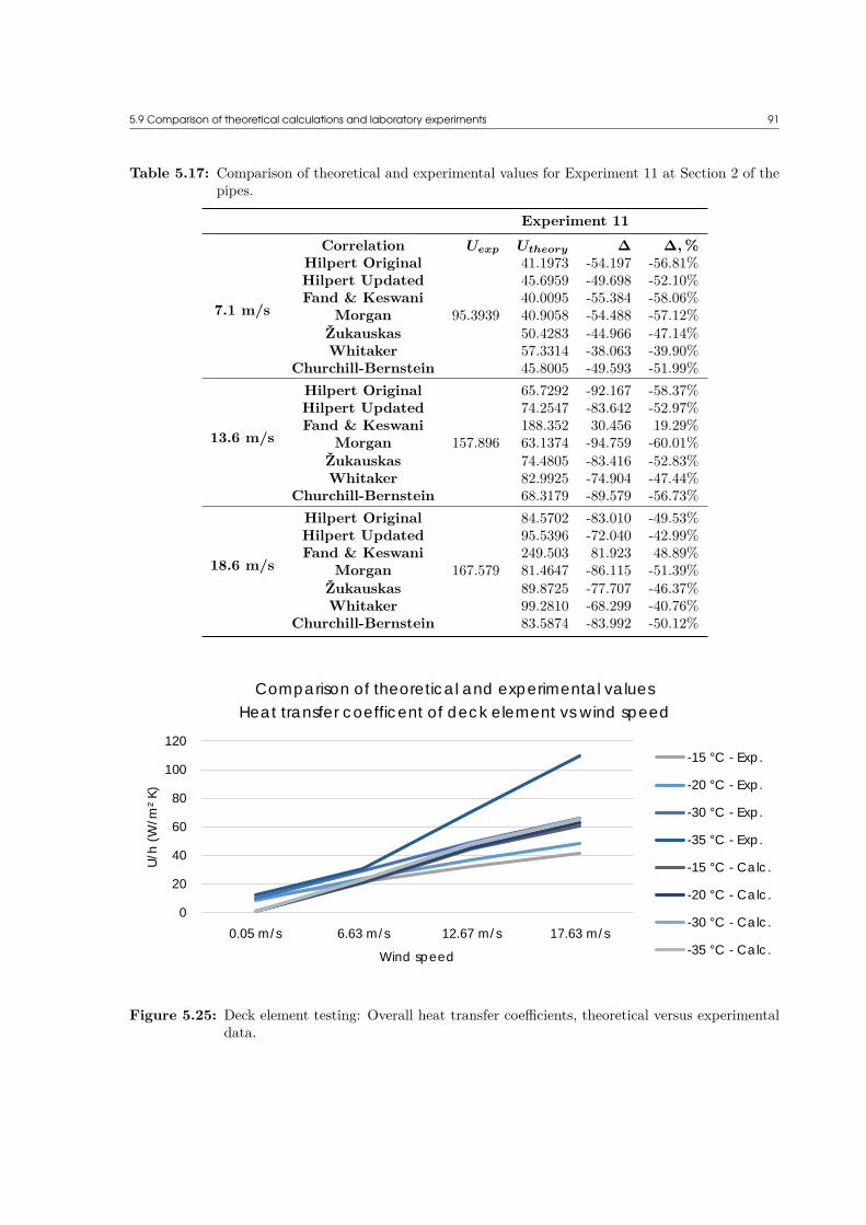
5.9 Comparison of theoretical calculations and laboratory experiments 91
Table 5.17: Comparison of theoretical and experimental values for Experiment 11 at Section 2 of thepipes.
Experiment 11Correlation Uexp Utheory ∆ ∆, %
7.1 m/s
Hilpert Original
95.3939
41.1973 -54.197 -56.81%Hilpert Updated 45.6959 -49.698 -52.10%Fand & Keswani 40.0095 -55.384 -58.06%
Morgan 40.9058 -54.488 -57.12%Žukauskas 50.4283 -44.966 -47.14%Whitaker 57.3314 -38.063 -39.90%
Churchill-Bernstein 45.8005 -49.593 -51.99%
13.6 m/s
Hilpert Original
157.896
65.7292 -92.167 -58.37%Hilpert Updated 74.2547 -83.642 -52.97%Fand & Keswani 188.352 30.456 19.29%
Morgan 63.1374 -94.759 -60.01%Žukauskas 74.4805 -83.416 -52.83%Whitaker 82.9925 -74.904 -47.44%
Churchill-Bernstein 68.3179 -89.579 -56.73%
18.6 m/s
Hilpert Original
167.579
84.5702 -83.010 -49.53%Hilpert Updated 95.5396 -72.040 -42.99%Fand & Keswani 249.503 81.923 48.89%
Morgan 81.4647 -86.115 -51.39%Žukauskas 89.8725 -77.707 -46.37%Whitaker 99.2810 -68.299 -40.76%
Churchill-Bernstein 83.5874 -83.992 -50.12%
0
20
40
60
80
100
120
0.05 m/s 6.63 m/s 12.67 m/s 17.63 m/s
U/h
(W
/m²
K)
Wind speed
Comparison of theoretical and experimental values
Heat transfer coefficent of deck element vs wind speed
-15 °C - Exp.
-20 °C - Exp.
-30 °C - Exp.
-35 °C - Exp.
-15 °C - Calc.
-20 °C - Calc.
-30 °C - Calc.
-35 °C - Calc.
Figure 5.25: Deck element testing: Overall heat transfer coefficients, theoretical versus experimentaldata.

92 5 Results
0
200
400
600
800
1000
1200
1400
1600
0.05 m/s 6.63 m/s 12.67 m/s 17.63 m/s
Po
we
r c
on
sum
ptio
n (
W)
Wind speed
Comparison of theoretical and experimental values
Deck element power consumption vs wind speed
-15 °C - Exp.
-20 °C - Exp.
-30 °C - Exp.
-35 °C - Exp.
-15 °C - Calc.
-20 °C - Calc.
-30 °C - Calc.
-35 °C - Calc.
Figure 5.26: Deck element testing: Total power consumption, theoretical versus experimental data.
Table 5.18: Comparison of theoretical and experimental values for deck element testing.
Common Experimental CalculatedT∞,set u∞ T∞ Ts,avg Uexp W ∆W hcalc qtot qconv
-15
0.05 -13.8 20.0 9.8 936.0 0.0 0.8 422.3 36.86.63 -13.9 3.7 21.6 1076.0 140.0 21.1 508.2 228.6
12.67 -13.5 -1.2 32.3 1123.3 187.3 44.1 587.3 376.517.63 -13.0 -3.2 41.3 1151.7 215.7 61.0 648.9 472.7
-20
0.05 -18.9 21.3 8.3 947.3 0.0 0.8 510.2 43.96.63 -19.2 -2.0 24.2 1175.3 228.0 21.8 492.5 228.5
12.67 -19.0 -7.2 36.9 1232.3 285.0 45.3 578.8 377.317.63 -18.9 -9.7 48.5 1263.7 316.3 62.6 618.7 459.2
-30
0.05 -29.2 9.5 9.8 1071.3 0.0 0.8 449.6 42.86.63 -27.8 -12.9 29.1 1231.3 160.0 23.2 424.3 209.0
12.67 -27.9 -18.4 49.3 1320.7 249.3 47.5 473.3 326.017.63 -29.6 -22.4 66.1 1362.0 290.7 65.7 484.8 391.7
-35
0.05 -27.8 4.5 12.3 1123.7 0.0 0.8 358.9 35.76.63 -27.3 -12.6 30.9 1291.5 167.8 23.2 413.6 205.9
12.67 -30.6 -23.6 70.5 1399.0 275.3 48.4 333.2 248.417.63 -26.9 -22.4 109.3 1409.0 285.3 65.4 272.9 242.9
5.10 Comparison of experimentsFig. 5.27 shows a comparison of the average overall heat transfer coefficient across the pipe forExperiment 1, 4, 5, 6 and 11. The Experiment 11 is significantly higher than the other experiments, soFig. 5.28 shows a comparison of Experiment 1, 4, 5 and 6. Tab. 5.19 presents a comparison of thedifference between Experiment 1 and Experiment 4, 5 and 6.

5.10 Comparison of experiments 93
0.00
20.00
40.00
60.00
80.00
100.00
120.00
140.00
160.00
180.00
200.00
0 m/s 5 m/s 10 m/s 15 m/s
U (
W/m
² K
)
Average overall heat transfer coefficients at Section 2
Experiment 1
Experiment 4
Experiment 5
Experiment 6
Experiment 11
Figure 5.27: Comparison of Experiment 1, 4, 5, 6 and 11.
2.10
2.20
2.30
2.40
2.50
2.60
2.70
2.80
0 m/s 5 m/s 10 m/s 15 m/s
U (
W/m
² K
)
Average overall heat transfer coefficients at Section 2
Experiment 1
Experiment 4
Experiment 5
Experiment 6
Figure 5.28: Comparison of Experiment 1, 4, 5 and 6.

945
Results
Table 5.19: Comparison of Experiment 1, 4, 5, 6.
Exp. 1 Experiment 4 Experiment 5 Experiment 6Uexp Uexp ∆ ∆, % Uexp ∆ ∆, % Uexp ∆ ∆, %
0 m/sRun 1 2.586 2.577 0.009 0.34% 2.576 0.009 0.35% 2.313 0.273 11.80%Run 2 2.583 2.543 0.040 1.59% N/A N/A N/A 2.383 0.200 8.39%Run 3 2.488 2.537 -0.048 -1.91% N/A N/A N/A 2.343 0.145 6.20%
Average 2.551 2.552 0.000 -0.02% 2.576 -0.025 -0.97% 2.346 0.206 8.76%
5 m/sRun 1 2.884 2.865 0.019 0.66% 2.879 0.004 0.14% 2.632 0.252 9.57%Run 2 2.892 2.922 -0.030 -1.02% N/A N/A N/A 2.705 0.187 6.91%Run 3 2.794 2.864 -0.070 -2.43% N/A N/A N/A 2.628 0.166 6.30%
Average 2.856 2.883 -0.027 -0.95% 2.879 -0.024 -0.82% 2.655 0.201 7.58%
10 m/sRun 1 3.028 2.986 0.042 1.41% 3.033 -0.006 -0.20% 2.665 0.362 13.58%Run 2 2.978 3.024 -0.046 -1.52% N/A N/A N/A 2.752 0.226 8.21%Run 3 2.886 2.945 -0.059 -2.00% N/A N/A N/A 2.692 0.193 7.18%
Average 2.962 2.984 -0.022 -0.73% 3.033 -0.071 -2.34% 2.703 0.260 9.61%
15 m/sRun 1 3.087 3.019 0.068 2.26% 3.007 0.080 2.67% 2.712 0.375 13.83%Run 2 2.956 3.037 -0.081 -2.67% N/A N/A N/A 2.766 0.189 6.85%Run 3 3.037 2.979 0.058 1.94% N/A N/A N/A 2.729 0.308 11.29%
Average 3.026 3.011 0.014 0.47% 3.007 0.019 0.62% 2.735 0.290 10.60%

5.11 Statistics from field testing 95
5.11 Statistics from field testingStatistics from the field testing is presented in Tab. 5.20. A time series plot of the overall heattransfer coefficient versus wind speed is presented for the uninsulated 50 mm pipe in Fig. 5.29 andthe insulated 50 mm pipe in Fig. 5.30. Similarly, for temperatures a time series plot is presented forthe uninsulated 50 mm pipe in Fig. 5.31 and for the insulated 50 mm pipe in Fig. 5.32
0.0
0.5
1.0
1.5
2.0
2.5
3.0
3.5
4.0
4.5
5.0
0.00
2.00
4.00
6.00
8.00
10.00
12.00
14.00
Win
d s
pe
ed
m/s
U (
W/m
² K
)
Time
Overall heat transfer coefficent versus wind speed, uninsulated pipe
Uninsulated pipe Wind speed
Figure 5.29: Time series plot of overall heat transfer coefficient versus wind speed for the uninsulatedpipe.
0.0
0.5
1.0
1.5
2.0
2.5
3.0
3.5
4.0
4.5
5.0
0.00
0.20
0.40
0.60
0.80
1.00
1.20
1.40
1.60
1.80
2.00
Win
d s
pe
ed
m/s
U (
W/m
² K
)
Time
Overall heat transfer coefficent versus wind speed, insulated pipe
Insulated pipe Wind speed
Figure 5.30: Time series plot of overall heat transfer coefficient versus wind speed for the insulatedpipe.

96 5 Results
0.0
1.0
2.0
3.0
4.0
5.0
6.0
7.0
8.0-20
-10
0
10
20
30
40
m/s
°C
Time
Temperature versus wind speed, insulated pipe
Sensor 13
Sensor 14
Sensor 15
Sensor 16
Sensor 17
Sensor 18
AmbientT
Wind speed
Note:
Sensor 13-18 and
AmbientT follow
left Y-axis
Figure 5.31: Time series plot of temperatures versus wind speed for the uninsulated pipe.
0.0
1.0
2.0
3.0
4.0
5.0
6.0
7.0
8.0-20
0
20
40
60
80
100
120
m/s
°C
Time
Temperature versus wind speed, insulated pipe
Sensor 1
Sensor 2
Sensor 3
Sensor 4
Sensor 5
Sensor 6
AmbientT
Wind speed
Note:
Sensor 1-6 and
AmbientT follow
left Y-axis
Figure 5.32: Time series plot of temperatures versus wind speed for the for the insulated pipe.

5.11 Statistics from field testing 97
Table 5.20: Statistics from field testing, overall heat transfer coefficients and temperatures.
U (W/m2 · K) T ( C)Min Max Avg St. Dev Min Max Avg St. Dev
Uninsulated
Entire pipe 4.57 13.18 7.43 1.59 -3.24 22.81 7.81 4.46Top 4.30 13.05 6.93 1.49 -0.89 22.81 8.93 4.55
Bottom 4.83 20.34 8.04 1.83 -3.24 18.14 6.69 4.08Section 1 4.33 15.45 7.78 1.72 -2.86 20.74 7.15 4.16Section 2 4.51 13.10 7.27 1.55 -3.24 22.81 8.14 4.63Section 3 4.57 13.78 7.28 1.58 -2.22 21.04 8.14 4.52
Insulated
Entire pipe 1.40 1.74 1.58 0.06 50.26 78.93 62.41 6.11Top 1.38 1.70 1.55 0.06 52.13 78.93 62.45 5.85
Bottom 1.42 1.78 1.61 0.07 50.26 76.50 61.12 6.10Section 1 1.47 1.86 1.66 0.07 50.26 69.96 58.82 4.29Section 2 1.30 1.58 1.45 0.05 61.00 78.93 68.61 4.16Section 3 1.45 1.80 1.64 0.07 52.13 70.10 59.78 4.24

98 5 Results
5.12 Estimated time to freezeThe estimated time to freeze the pipes used in the experiments are calculated, and is presented in Tab.5.21 & 5.22. Additional calculations for different diameters and insulation thicknesses can be foundin Appendix D.
Table 5.21: Time required to freeze 25 mm and 50 mm pipe.
Common Hilpert Hilpert Upd. Fand & Keswani MorganDo u∞ tins U ttf, h U ttf, h U ttf, h U ttf, h
25 0.05 0 4.38 7.99 4.86 7.20 4.22 8.29 4.25 8.2310 1.40 24.88 1.47 23.79 1.38 25.28 1.39 25.18
25 6.63 0 51.72 0.77 57.35 0.71 49.90 0.80 50.79 0.7810 2.35 14.81 2.37 14.73 2.35 14.84 2.35 14.82
25 12.63 0 76.93 0.55 85.29 0.51 74.66 0.57 76.28 0.5610 2.40 14.52 2.41 14.45 2.46 14.16 2.40 14.54
25 17.67 0 94.58 0.47 104.85 0.44 92.07 0.48 94.26 0.4710 2.42 14.39 2.43 14.34 2.47 14.11 2.42 14.40
50 0.05 0 3.03 25.37 3.36 22.90 2.92 26.28 2.95 26.0310 1.33 56.97 1.40 54.01 1.30 58.05 1.31 57.71
50 6.63 0 39.72 2.41 44.04 2.23 38.56 2.47 39.41 2.4310 2.59 29.48 2.62 29.24 2.72 28.11 2.59 29.49
50 12.63 0 62.52 1.72 70.60 1.58 177.37 0.94 60.04 1.7710 2.67 28.61 2.69 28.47 2.76 27.77 2.67 28.66
50 17.67 0 81.85 1.43 92.42 1.33 239.07 0.83 78.84 1.4710 2.70 28.31 2.71 28.20 2.77 27.66 2.70 28.35

5.12 Estimated time to freeze 99
Table 5.22: Time required to freeze 25 mm and 50 mm pipe.
Common Morgan Žukauskas Whitaker Churchill-BernsteinDo u∞ tins U ttf, h U ttf, h U ttf, h U ttf, h
25 0.05 0 4.25 8.23 4.23 8.27 4.97 7.05 4.85 7.2310 1.39 25.18 1.39 25.05 1.50 23.18 1.47 23.74
25 6.63 0 50.79 0.78 64.51 0.64 72.01 0.59 58.99 0.6910 2.35 14.82 2.38 14.65 2.39 14.59 2.37 14.73
25 12.63 0 76.28 0.56 94.82 0.47 103.42 0.44 85.52 0.5110 2.40 14.54 2.42 14.43 2.42 14.40 2.41 14.48
25 17.67 0 94.26 0.47 115.86 0.40 124.99 0.38 104.55 0.4410 2.42 14.40 2.43 14.35 2.43 14.33 2.42 14.38
50 0.05 0 2.95 26.03 2.99 25.65 3.61 21.37 3.38 22.7510 1.31 57.71 1.33 56.97 1.47 51.58 1.41 53.64
50 6.63 0 39.41 2.43 48.94 2.05 53.30 1.93 44.11 2.2210 2.59 29.49 2.63 29.09 2.64 28.96 2.61 29.28
50 12.63 0 60.04 1.77 71.96 1.56 76.80 1.49 65.40 1.6710 2.67 28.66 2.68 28.53 2.69 28.46 2.67 28.63
50 17.67 0 78.84 1.47 87.95 1.37 93.00 1.32 81.07 1.4410 2.70 28.35 2.70 28.31 N/A N/A 2.70 28.37

100

CHAPTER 6Discussion
6.1 Pipes
6.1.1 Experiment 1Experiment 1 was used as the baseline case for 50 mm insulated pipes, and is used for comparing thedifferent surface coatings. In Fig. 5.2 the difference in the overall heat transfer coefficient from thetop to the bottom of the pipe is shown. The heating element was positioned in the center of the pipe,and from Tab. 5.2 it is found that the temperature difference from the bottom of the pipe and thetop is around 2 C. This temperature difference is already mitigated in industrial applications, wherethe common practice is to install the heating element at the bottom of the pipe. In Fig. 5.1 a sketchof the different sections is shown. Fig. 5.3 shows the temperature difference between Section 1, 2 and3, and it shows the difference in the overall heat transfer coefficient from the center to the sides. Whencomparing temperatures at Section 1 and 3 with temperatures at Section 2, a difference of 5-10 C wasobserved. This affected the theoretical calculations during the analysis of the data, as the calculatedsurface temperature of the insulation was found to be well below the ambient temperature. Fig. 5.2also shows that the increase from 0 m/s to 5 m/s wind speed is the most significant, and the increasefrom 5 m/s to 10 m/s and 15 m/s has a lower gradient.
6.1.2 Experiment 2Experiment 2 tested two insulated 50 mm pipes that were positioned in line. The purpose of thisexperiment was to validate the effect of staggered flow. It is assumed that the pipe that was positioneddirectly in front of the wind nozzle will have the same heat loss as a single pipe, but the effect on thesecond pipe is unknown. This experiment is discussed in detail in Peechanatt (2016).
6.1.3 Experiment 3Experiment 3 tested three insulated 50 mm pipes that were positioned in line. The purpose of thisexperiment was to validate the effect of staggered flow across pipes that were located in very closeproximity. It is assumed that the pipe that was positioned directly in front of the wind nozzle willhave the same heat loss as a single pipe, but the effect on the second and third pipe is unknown. Thisexperiment is discussed in detail in Peechanatt (2016).
6.1.4 Experiment 4Experiment 4 tested the effect of ice glazing on the exterior of the insulation. The goal was to seewhether the increased roughness of the surface affected the overall heat transfer coefficient. The icewas applied using a spray bottle filled with fresh water. The water was applied in multiple steps, withfive minutes between each spray. The resulting ice was very uneven and would simulate a pipe exposedto sea spray. A picture of the pipe at the start of the testing is shown in Fig. 6.1. The experimentwas considered to be a partial success, and it should be noted that when the pipes where removed afterthe experiment the ice glazing was no longer present. The reason for this is uncertain as no visualobservations were made of the pipe after the first run, but from the temperatures in Tab. 5.3 there

102 6 Discussion
does not appear to be a major difference in temperatures. It could be that surface temperature ofthe insulation reached a temperature above zero at 0 m/s wind speed, and this caused the ice to meltclose to the insulation and fall off the insulation. Another reason could be that the ice was removedmechanically at higher wind speeds.
Figure 6.1: Pipe with ice glazing as tested ©Bjarte Odin Kvamme.
From Fig. 5.4 & 5.5 we see that the overall heat transfer coefficients have the same profile as inExperiment 1. Looking at the comparison plot in Fig. 5.28 confirms this.
6.1.5 Experiment 5Experiment 5 tested the effect of an even layer of ice, or an ice coating on the exterior of the insulation.The goal was to see if a layer of ice would affect the overall heat transfer coefficient of the pipe. As the icelayer was even and smooth, it is assumed that this would primarily have an insulating effect. Experiment5 was performed after Experiment 4, and only one run was performed, as the ice in Experiment 4 haddisappeared during the experiment. After this run, the ice layer was still present on the pipe, but theremaining runs were not performed.
The plots in Fig. 5.6 & 5.7 show that Experiment 5 follows the same trend as Experiment 1 and4, but the overall heat transfer coefficent at 15 m/s wind speed is lower than that of 10 m/s wind speed.This could be a one-time deviation which would have averaged out if more runs had been performed.When looking at the comparison plot in Fig. 5.28 we see that the overall heat transfer coefficient at10 m/s is higher than that of Experiment 1 and 4, while the other wind speeds show similar values.
6.1.6 Experiment 6As Experiment 4 was not a complete success, it was decided to try another configuration where thesurface roughness would not melt. For Experiment 6, quartz particles ranging from 0.8 to 1.2 mm insize was adhered to the insulation of the pipe to simulate a pipe that had been exposed for a long periodof time with no maintenance. A picture of the pipe is shown in Fig. 6.2. In hindsight, the methodused to apply the quartz was far from ideal, and the glue and quartz appears to have added a layer
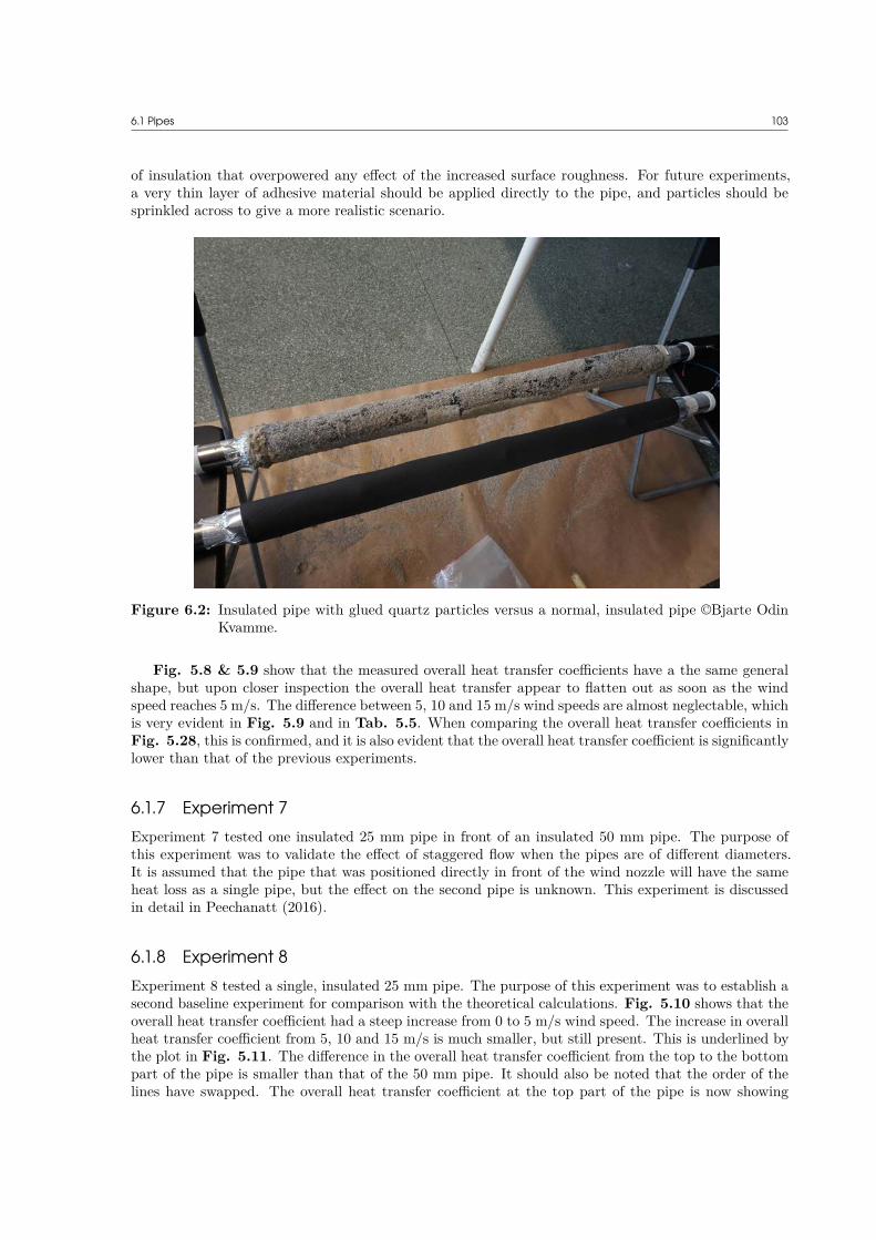
6.1 Pipes 103
of insulation that overpowered any effect of the increased surface roughness. For future experiments,a very thin layer of adhesive material should be applied directly to the pipe, and particles should besprinkled across to give a more realistic scenario.
Figure 6.2: Insulated pipe with glued quartz particles versus a normal, insulated pipe ©Bjarte OdinKvamme.
Fig. 5.8 & 5.9 show that the measured overall heat transfer coefficients have a the same generalshape, but upon closer inspection the overall heat transfer appear to flatten out as soon as the windspeed reaches 5 m/s. The difference between 5, 10 and 15 m/s wind speeds are almost neglectable, whichis very evident in Fig. 5.9 and in Tab. 5.5. When comparing the overall heat transfer coefficients inFig. 5.28, this is confirmed, and it is also evident that the overall heat transfer coefficient is significantlylower than that of the previous experiments.
6.1.7 Experiment 7Experiment 7 tested one insulated 25 mm pipe in front of an insulated 50 mm pipe. The purpose ofthis experiment was to validate the effect of staggered flow when the pipes are of different diameters.It is assumed that the pipe that was positioned directly in front of the wind nozzle will have the sameheat loss as a single pipe, but the effect on the second pipe is unknown. This experiment is discussedin detail in Peechanatt (2016).
6.1.8 Experiment 8Experiment 8 tested a single, insulated 25 mm pipe. The purpose of this experiment was to establish asecond baseline experiment for comparison with the theoretical calculations. Fig. 5.10 shows that theoverall heat transfer coefficient had a steep increase from 0 to 5 m/s wind speed. The increase in overallheat transfer coefficient from 5, 10 and 15 m/s is much smaller, but still present. This is underlined bythe plot in Fig. 5.11. The difference in the overall heat transfer coefficient from the top to the bottompart of the pipe is smaller than that of the 50 mm pipe. It should also be noted that the order of thelines have swapped. The overall heat transfer coefficient at the top part of the pipe is now showing

104 6 Discussion
a higher heat loss than the bottom part, which is the opposite from the results found for the 50 mmpipes.
6.1.9 Experiment 9Experiment 9 tested two insulated 25 mm pipes positioned in line. The purpose of this experiment wasto validate the effect of staggered flow, and see whether the effect on 25 mm pipes are different thanthe 50 mm pipes tested in Experiment 2. This experiment is discussed in detail in Peechanatt (2016).
6.1.10 Experiment 10Experiment 7 tested one insulated 50 mm pipe in front of an insulated 25 mm pipe. The purpose ofthis experiment was to validate the effect of staggered flow when the pipes are of different diameters.The 50 mm pipe is positioned in front of the 25 mm pipe, and should disturb the flow of air. Thisexperiment is discussed in detail in Peechanatt (2016).
6.1.11 Experiment 11Experiment 11 tested a single, uninsulated 50 mm pipe. The goal of this experiment was to establishhow big a difference insulation makes to the heat loss of a pipe. Fig. 5.12 shows that the overall heattransfer coefficient increases almost linearly with the wind speed. Fig. 5.13 shows that the differencebetween each section is smaller than that of the insulated pipe, but some variation is still observed,especially at 5 and 10 m/s wind speeds. One important aspect to note is that the temperature sensorsmight have been cooled down directly, and thus not accurately representing the pipe temperature. Asthe temperature sensors where mounted on the exterior of the pipe, they were directly exposed tothe wind. The overall heat transfer coefficient obtained from the experimental data are therefore notassumed to be accurate, as the temperature of the pipe is likely to be higher than measured.
In Tab. 5.7 it is found that the temperatures at 5, 10 and 15 m/s wind speeds do not changesignificantly. The sharp increase in the overall heat transfer coefficient is caused by the way the overallheat transfer coefficient is calculated. As the temperature difference approaches zero, the overall heattransfer coefficient will approach infinity. Thus, a very small difference in temperature will have asignificant impact on the overall heat transfer coefficient.
6.1.12 Comparison with theoretical valuesTheoretical calculations were performed for the scenarios tested in Experiment 1, 8 and 11. Completedatasets with the theoretical values are found in Chapter 5.8. For the insulated, 50 mm pipe, thetheoretical and experimental values are very close, and the deviation between the theoretical and ex-perimental values is between 0.40 % to 5.79 % with an average of 1.74 % depending on the correlationused. It can also be observed in Tab. 5.16 that the deviation between experimental and theoreticalvalues decreases at higher wind speeds, but the Nusselt numbers calculated using Fand & Keswani showvalues that are significantly higher than the other correlations. This is also visible in Fig. 5.17.
For the uninsulated 50 mm pipe, the deviations are considerably higher, as illustrated in Fig. 5.24.The Fand & Keswani correlation has a very large deviation for this experiment. As the correlationshows fair numbers at 7.1 m/s wind speed, the reason for this deviation is believed to be that theReynolds number exceeds 40 000 for wind speeds of 13.6 and 18.6 m/s, and this results in a new setof constants in the formulas. In Tab. 5.15 the experimental values are found to be 43 % higher onaverage compared to the theoretical values. It is believed that this difference is caused by incorrecttemperature measurements in the experiments, and not inaccuracy in the theoretical calculations.
For the insulated 25 mm pipe, the deviations are higher throughout, and the correlations consistentlygive a lower overall heat transfer coefficient. From Tab. 5.15, the deviation is found to range from -4.54% and -0.72 %, with an average deviation of -2.91 %. It is noted that the Fand & Keswani correlation

6.2 Deck element 105
gives values that are closer to the experimental values. However, the increase from 7.1 to 13.6 m/s windspeed is very significant and is also caused by the Reynolds number exceeding 40 000.
6.1.13 Field testingField experiments were performed aboard KV Svalbard as part of SARex. The purpose was to measurereal-life conditions for a pipe, and estimate the heat loss. In Fig. 5.29 a plot of the overall heattransfer coefficient versus the measured wind speed is presented. The wind speed sensor used was notvery accurate, and requires a minimum of 0.8 m/s wind speed before voltage is outputted to the datalogger. When combined with a sample resolution of 30 seconds, this becomes very evident in Fig.5.29 & 5.30, as the measured wind speed frequently drops to 0 m/s. Comparing the insulated pipeand uninsulated pipe does however reveal a very distinct difference between the overall heat transfercoefficient between the two. The overall heat transfer coefficient of the uninsulated pipe range from4.57 to 13.18 W/(m2 · K), while the insulated pipe range from 1.40 to 1.74 W/(m2 · K). Fig. 5.30shows that the insulated pipe is not significantly affected by the wind, while the uninsulated pipe asshown in Fig. 5.29 has very large changes.
Fig. 5.31 shows that the pipe temperature dropped below 0 C on several occasions, while theinsulated pipe temperatures as shown in Fig. 5.32 never drop below 50 C.
6.1.14 Estimated time to freezeBased on the overall heat transfer coefficients, the required time to freeze was calculated and is presentedin Tab. 5.21 & 5.22. All seven correlations have very similar values for the estimated time to freeze.The time to freeze calculations take into consideration the time required for the center of the pipe tofreeze and reach -1 C. In Kvamme (2014) it was found that the formation of ice would differ basedon the ambient temperature and wind conditions. If the heat transfer from the outer pipe wall to theenvironment is sufficiently high, ice will form from the inner pipe wall and form inwards. If the heattransfer is more gradual, the cooled water could circulate inside the pipe via means of convection andthe ice might form as a floating layer on top of the water. In either case, the formation of ice is undesiredas this can cause hazards to personnel and equipment damage. The difference in heat loss between anuninsulated and insulated pipe is very evident, and clearly demonstrates the benefit of insulating pipes.Even a very modest insulation thickness of 5 mm increases the required time to freeze for a 25 mm pipein 5 m/s wind speed from less than one hour to approximately seven hours. If the insulation thicknessis increased to 10 mm, the required time to freeze increases to approximately 15 hours. If the pipefreezes, it could rupture due to the volume expansion as water transforms into solid state. Even if thepipe does not rupture, a significant amount of energy is required to de-thaw the pipe, and can be verydifficult to achieve, depending on the ease of access to the pipe. This can be a big concern, especiallyfor complex piping arrangements as typically found in oil and gas production facilities.
6.2 Deck elementTemperature measurements in Tab. 5.8 & 5.9 show that the deck element was able to maintainpositive temperatures at 0 m/s wind speed down to the maximum tested temperature of -35 C. At 5m/s wind speed, the deck element was able to maintain a positive temperature at -15 C. At -20 C someareas of the deck element maintained a positive temperature, but the average surface temperature wasbelow 0 C. At higher wind speeds or lower temperatures, the deck element was not able to maintaina positive surface temperature.
The deck elements showed a steady increase in power consumption as the wind speed was increased.The increased power consumption correlated well with the calculated convective heat transfer. For theexperiments performed at -15 C, -30 C and -35 C insufficient time was allocated to each experiment,and the deck element was not able to stabilize properly before the change in wind speed was made. This

106 6 Discussion
resulted in some rather fluctuating measurements at all wind speeds. Prior to the experiment at -20 Cthe data analysis had started, and it was discovered that the values were far from uniform. The timeallocated for each experiment was increased, and the values obtained for this experiment were muchmore consistent between each run, but still not perfect.
In hindsight, four to six hours should have been allocated at each wind speed to allow the tempera-tures time to distribute properly in the deck element. The thermal capacity of the deck element resultedin more time than expected to reach steady-state conditions. The temperature sensors inside the deckelement should also have been utilized, as well as a monitoring system that made it possible to monitorthe temperature development over a longer period of time. This was done for the pipe experiments,and made it possible to identify when the pipe temperatures had stabilized properly.
As a result of these shortcomings, the overall heat transfer coefficient found from the experimentaldata does not correlate well with the theoretical data. The theoretical calculations assume steady-state conditions where the temperatures have reached an equilibrium with the environment. The largedeviations between each run prove that this was not the case. The self-regulating design of the deckelement could also be a source of error, and the critical Reynolds number Rex,c is also likely to be lowerthan the assumed value of 5 × 10⁵ due to the roughness of the deck element. The heat tracing willuse as much power as possible until the temperature of the heat tracing reaches 60 C. Once 60 C isreached, the heat tracing will increase the resistance and reduce the power consumption.
The power consumption at no wind conditions was found to be significantly higher than expected,and despite intense calculations and assumptions, the source(s) of the heat loss remains unidentified.No measurements were performed to establish the internal temperature of the deck element, but it isassumed that this temperature would be higher than the temperature measured at the surface of thedeck element using the infra-red camera. The deck element was mounted on a wooden pallet to reducethe conductive heat transfer to the floor in the climate laboratory, but the deck element was larger thanthe pallet, so some convective heat transfer took place on the underside of the deck element.
Conversation with Trond Spande, formerly of GMC Maritime AS revealed that the power consump-tions and surface temperatures measured at 5 m/s were corresponding with his experience. He alsonoted that if a comparison with theoretical values should be performed, heat tracing with a constantresistance should be used to allow for more controlled testing. It was also recommended to position thedeck element behind a wall or a box to prevent wind. Even the wind generated by the evaporators hada noticeable impact on the heat loss.
6.2.1 Key elements for optimal deck element designBased on our findings, the following key elements should be considered:
• Heat loss to the bottom of the deck element.
• Use of insulating materials at the bottom of the deck element.
• Use of heat conducting materials to distribute heat.
• Anti-slip surface coating.
• Drainage paths for melted water.
• Ease of installation.
• Intelligent control systems to increase power efficiency.
Based on the comparison of theoretical calculations and experimental values, only 1/3 of the mea-sured power consumption should be lost through convective heat transfer from the surface. This willof course depend on the wind speed used, but even at a wind speed of 15 m/s and an ambient temper-ature of -20 C, the estimated convective heat transfer found to be 350 W for a 1 m2 plate. The ratedmaximum power of GMC’s deck element was 1400 W, and should have plenty of power if this was the

6.2 Deck element 107
only source of heat loss. The sources for the heat loss should be investigated thoroughly, as this willhave a huge impact on operational cost and environmental discharges. Preventing the formation of iceand snow on the deck surface is vital to maintain a safe working environment for the crew, but thisshould be done as efficiently as possible.
It is assumed that a large portion of the heat is lost through the bottom of the deck element, viaconductive heat transfer to the installation surface. In the tested element, a steel plate was used as thefoundation for the moulded epoxy, as this represents normal installation on a vessel. This heat transferwill be used to heat up the hull or superstructure of the vessel, which should not be the goal of the heattracing in the deck elements.
Internally in the deck element, conductive materials should be used to evenly distribute the heatgenerated by the heat tracing. This is present in the deck element provided by GMC, and the thermalimages showed a very even temperature distribution on the surface. This was not done on the helicopterdeck of KV Svalbard, and the gridded structure of the heat tracing is clearly visible on the thermalimage of the helicopter deck as shown in Fig. 6.6.
Anti-slip surface coating should be used to provide a safe working environment. This is alreadyindustry practice, and should be continued.
The deck element tested did not have any method of draining melted water incorporated. Thisshould be considered for future designs. If the melted water is not removed from the deck surface, theheat from the deck element will be used for heating and evaporating of the water. This energy wouldbe far better used for melting snow and ice, and not heating up water. Different methods of doing thisis possible, depending on the requirements of the deck. One method would be to have channels in thedeck element that guides the water away from the deck elements and to a drainage pipe or back intosea. Another option would be to mount the deck elements on a small incline so that water will naturallydrain away.
For vessels operating primarily in polar regions, permanently installed heat tracing is not a majorconcern for new constructions as a deck surface is needed in any case. For modifying and winterizationof existing vessels, standalone heated deck elements as shown in Fig. 6.3 can be utilized with greatease. These deck elements are bolted into place, and can be removed if damaged or worn down.
Intelligent control systems should be designed and used to minimize the waste of energy. Thiswill have a higher installation and procurement cost, but should if properly implemented reduce theoperational costs significantly, and the added cost of installation and procurement will be recoveredquickly.
6.2.2 Experiences from laboratory experimentsThe Polar Code does not require heat traced deck elements for escape routes specifically, only that”... means shall be provided to remove or prevent ice and snow accumulation from accesses.” (IMO,2016). The Polar Service Temperature (PST) requirements in the Polar Code, state that the designtemperature shall be at least -10 C lower than the expected Mean Daily Low Temperature (MDLT).DNV GL (2015) requires that the heating capacity should be established with a heat balance calculation.If uninsulated and exposed to wind, the heat balance should also include the wind cooling effect basedon a nominal wind speed of 20 m/s. The use of a nominal wind speed as the requirement allows forsome flexibility in the requirements by DNV GL in how the heat tracing is implemented. It is also seenin the results that the increase from 0 m/s wind speed to 5 m/s wind speed is higher than from 5 m/sto 10 m/s or 15 m/s. Fig. 6.3 shows that a deck element under testing for certification for the PolarCode had to be positioned inside pallet boxes to protect it from the wind caused by the evaporators. Ifleft unprotected from the wind, the deck element would not satisfy the requirements in the Polar Code.
It was interesting to observe that the deck element has to be completely protected from wind to beable to satisfy the requirements in the Polar Code. The experiments performed on the deck elementrevealed that the deck element was able to maintain a positive surface temperature in 0 m/s windspeeds all the way down to -35 C, but only at -15 C if the wind speed was 5 m/s or higher.

108 6 Discussion
Figure 6.3: Deck element inside pallet boxes to remove any wind from the evaporators. ©Bjarte OdinKvamme.
6.2.3 Experiences from KV SvalbardOn board the vessel KV Svalbard, examples of underpowered heat tracing was observed. The aft andhelicopter deck had heat tracing installed, supposedly rated at 400W/m2. This was the requirement fromDet Norske Veritas (now: DNV GL), who classed the vessel at the time of commissioning, 15.12.2001(NoCGV Svalbard, 2016). The heat tracing was not able to keep the deck surface ice and snow freewhile the vessel was in transit, or if the vessel was subjected to wind. Fig. 6.5 shows snow and iceaccumulating on the helicopter deck during the transit to Woodfjorden. Fig. 6.6 shows a thermalimage of the starboard side of the helicopter deck. The ambient temperature was -12 C, and the vesselwas moving at 13 knots. Once we arrived at our destination, the heat tracing was able to de-ice allsections of the deck.
Conversations with officers on board revealed that in rough conditions they have to cover the heli-copter deck with tarpaulin to remove the effect of the wind. This was done when they were expectinga helicopter, and would be difficult to achieve in case of an unexpected landing.

6.2 Deck element 109
Further conversations revealed that the power consumption of the heat tracing during bad weathercaused the transit speed to be reduced. The heat tracing used a considerable amount of power, whichreduced the available power to the azipod propulsion system. The officers noted that this could bemitigated by starting additional diesel engines to drive the generators, but this would again increasefuel consumption. When taking into consideration that the heat tracing was not even able to keep thesurfaces ice free, it is evident that this is not an optimal scenario.
Ice was also found to be forming on nozzles used in the vessels fire extinguishing system. The pipesused were insulated, but the diameter of the pipe used and the thickness of the insulation is not known.Fig. 6.4 shows a picture of a nozzle and some piping on the starboard side of KV Svalbard during thetransit to Woodfjorden. The fire extinguishing system was not tested, but conversion with the chiefengineer on board revealed that water was constantly circulated through the pipes to avoid freezing.
Figure 6.4: Ice accumulation on fire extinguishing nozzle on KV Svalbard. Picture taken in April2016, west of Ny Ålesund. Ambient temperature was -12 C and no wind apart from theair flow caused by the transit at 13 knots. ©Trond Spande.

110 6 Discussion
Figure 6.5: Snow and ice accumulation on the helicopter deck on KV Svalbard. Picture taken in April2016, west of Ny Ålesund. Ambient temperature was -12 C and no wind apart from theair flow caused by the transit at 13 knots. ©Trond Spande.
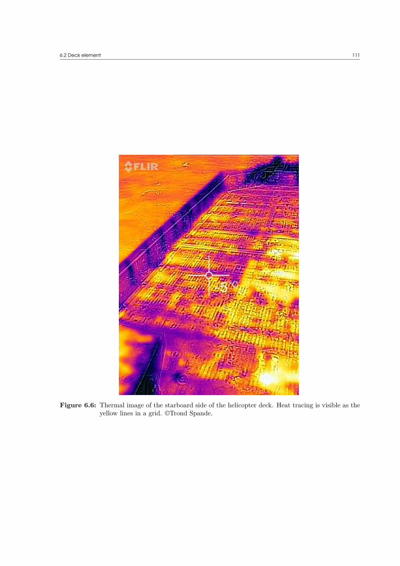
6.2 Deck element 111
Figure 6.6: Thermal image of the starboard side of the helicopter deck. Heat tracing is visible as theyellow lines in a grid. ©Trond Spande.

112

CHAPTER 7Conclusions
Based on the experimental data, all of the tested heat transfer correlations used for cylinders are foundto give accurate values for the overall transfer coefficient. For a 50 mm insulated pipe, the theoreticalvalues are found to be in the range of 0.40 % to 5.79 % off the experimental values. For a 25 mm insulatedpipe the theoretical values are found to be in the range of -4.54 % to -2.91 % off the experimental values.For the uninsulated pipe, the experimental values are significantly higher than the theoretical values.This is likely due to the way the temperature sensors were installed.
The overall heat transfer coefficient of an uninsulated pipe is found to increase significantly withincreasing wind speeds. For an insulated pipe, the overall heat transfer coefficient also increases, butonly by decimal points. Even at a very low wind speed of 0.05 m/s, the overall heat transfer coefficientof an uninsulated pipe is three times higher than that of an insulated pipe. The field experiments onKV Svalbard confirm this, and showed that the overall heat transfer coefficient for uninsulated pipeswere up to ten times higher than that of the insulated pipe. The field experiments were performedunder ideal conditions, and the difference would be much higher if the weather had been worse.
Based on this, it is recommended that all pipes used in superstructures in cold climates are insulated.If the pipes are exposed to wind this should be a requirement, as the heat transfer of an uninsulated pipeincreases dramatically even with low wind speeds. The effect of a rapidly changing heat transfer canhave a detrimental effect on complex systems where the fluid properties are important. De-thawing ofpipes takes a long time and can be difficult to perform under ideal conditions, and can pose a significantchallenge in complex piping arrangements.
The limited range of applicability of the Whittaker and Morgan correlations exclude them for recom-mended use. The Fand & Keswani correlation shows erratic behaviour at Reynolds numbers exceeding40 000, and is therefore excluded as well. The correlations based on Hilpert’s correlation are simple touse for hand-calculations, but the availability of computers and sufficiently powerful hand-held deviceshas reduced the importance of the ease of use in hand-calculations. All correlations apart from Fand& Keswani were found to be accurate for the tested configurations, and can easily be implemented inprogramming and spreadsheets. The recommended convective heat transfer correlation for cylinders ina cross-flow wind arrangement is therefore chosen to be the Churchill-Bernstein correlation, found inEquation (2.38). The Churchill-Bernstein correlation has the widest range of applicability, and is theeasiest to incorporate in spreadsheets and programs. This because it does not require the use of tablesfor looking up values or the calculation of fluid properties at different temperatures.
For flat plates, only one set of equations were found for the surface averaged Nusselt number duringthe literature review, and a comparison between different correlations has therefore not been performed.The comparison between the experimental values and the theoretical values showed that the theoreticalconvective heat loss was comparable to the increased power consumption of the deck element in wind, butthat a significant amount of heat loss is still unaccounted for under 0 m/s wind conditions. Observationson the KV Svalbard revealed that even air flows caused by the vessel in transit has a big impact on theheat loss of the deck. The heat tracing used in the deck elements were not able to provide sufficientde-icing, and tarpaulins were used to stop the effect from the wind if the helicopter deck was needed.
The fact that the Polar Code (IMO, 2016) does not take into account wind in the requirements forequipment operation is concerning. In all the experiments performed the effect of wind is significant,even at low velocities. When testing the deck elements, it was observed that the surface temperature ispositive at 0 m/s wind speed down to -35 C. When at 5 m/s or greater, a positive surface temperaturewas not observed. Thus, satisfying the requirements in the Polar Code might not ensure the desired

114 7 Conclusions
operational environment. DNV GL (2015) requires the use of a heat balance equation at a nominal windspeed of 20 m/s and should function much better in realistic conditions, depending on how nominal isdetermined.
7.1 Future workFor piping on oil and gas processing facilities, a flow assurance analysis should be performed. A com-parison should be performed between two facilities, one with insulated pipes and one with uninsulatedpipes.
A life cycle cost analysis should be performed to evaluate the costs associated with the use ofinsulated pipes versus uninsulated pipes. Insulated pipes will have a higher installation cost, butbased on the findings in this thesis, the savings in power consumption should make this a worthwhileinvestment.
A further analysis should be performed on the deck element under more controlled conditions andwith more measuring equipment. The theoretical convective heat transfer of a deck element is signifi-cantly lower than the measured power consumption, and despite the high surface roughness of the deckelement, all sources of heat loss can not be accounted for in a satisfying matter. The heat tracing in thisdeck element should not be self-regulating, and sufficient time should be allocated for the deck elementto reach equilibrium.
An case study of deck elements that are insulated from the vessel should also be performed. Thedesign tested is moulded directly on the vessel, which will result in large amounts of electricity usedonly to heat up the hull of the vessel. Insulating the deck element from the installation surface shouldhelp reduce the power consumption and result in a more economical design of the deck elements.
A study should be performed on how cold climate affects the nozzles used in fire extinguishingsystems. This thesis only considers piping, and none of the subsystems which are also required tomaintain a working fire extinguishing system. Nozzles aboard KV Svalbard showed icing, but thefunctionality of the system was not tested.

BibliographyAdafruit. (2015). Adafruit data logger shield. Retrieved March 27, 2016, from https://learn.adafruit.
com/adafruit-data-logger-shieldAhlenius, H. (2007). Trends in antarctic tourism. Figure. Retrieved May 12, 2015, from http://www.
grida.no/graphicslib/detail/trends-in-antarctic-tourism_1619Aosong Electronics Co. (2010). Digital-output relative humidity and temperature sensor/module DHT22.
Datasheet. Retrieved May 26, 2016, from https : / / www . sparkfun . com / datasheets / Sensors /Temperature/DHT22.pdf
Armacell Norway. (2016). Tekniske data - AF/Armaflex N. Datasheet. Retrieved May 29, 2016, fromhttp : / / local . armacell . com / fileadmin / cms / norway / products / product - catalogs - no / AF _Armaflex_N_Produktkatalog_2016_NW.pdf
ASHRAE. (2010). 2010 ASHRAE Handbook - Refrigeration - SI Edition. American Society of Heating,Refrigerating and Air-Conditioning Engineers, Inc.
Bird, K. J., Charpentier, R. R., Gautier, D. L., Houseknecht, D. W., Klett, T. R., Pitman, J. K.,… Wandrey, C. J. (2008). Circum-arctic resource appraisal: estimates of undiscovered oil and gasnorth of the arctic circle. Retrieved May 26, 2016, from http://pubs.usgs.gov/fs/2008/3049/fs2008-3049.pdf
Bowermaster, J. (2007). Special report: the sinking of the explorer. Retrieved May 7, 2016, from http://www.nationalgeographic.com/adventure/news/explorer-sinks-antarctica.html
Burton, M. (2016). Dallas temperature control library. Retrieved March 27, 2016, from http://milesburton.com/Main_Page?title=Dallas_Temperature_Control_Library
Çengel, Y. A. (2006). Heat and mass transfer: a practical approach. Boston: McGraw-Hill.Churchill, S. W. & Bernstein, M. (1977). A correlating equation for forced convection from gases and
liquids to a circular cylinder in crossflow. Journal of Heat Transfer, 99(2), 300–306. doi:10.1115/1.3450685
Comiso, J. C., Parkinson, C. L., Markus, T., Cavalieri, D. J., & Gersten, R. (2015). Current state ofthe sea ice cover. Figure. Retrieved May 12, 2015, from http://neptune.gsfc.nasa.gov/csb/index.php?section=234
DNV GL. (2015). Winterization for cold climate operations. DNV GL. Retrieved March 27, 2016, fromhttps://rules.dnvgl.com/docs/pdf/dnvgl/OS/2015-07/DNVGL-OS-A201.pdf
Dubey, B. (June 21, 2012). The rise of northern sea route. Presentation. Skuld.Fand, R. M. & Keswani, K. K. (1973). Recalculation of hilpert’s constants. Journal of Heat Transfer,
95(2), 224. doi:10.1115/1.3450030Fay, G., Karlsdöttir, A., & Bitsch, S. (2010). Observing trends and assessing data for arctic tourism.
Poster. University of Alaska Anchorage. Retrieved May 12, 2015, from http://www.iser .uaa.alaska.edu/Projects/SEARCH-HD/images/AON-SIP.tourism.poster.pdf
FLIR Systems, Inc. (2016). FLIR A315. Datasheet. Retrieved May 26, 2016, from http://support.flir.com/DsDownload/Assets/48001-1101-en-US_A4.pdf
Hilpert, R. (1933). Wärmeabgabe von geheizten drähten und rohren im luftstrom. Forsch. GebeiteIngenieurwes, 4, 215–224.
Hung, Y. C. & Thompson, D. R. (1983). Freezing time prediction for slab shape foodstuffs by animproved analytical method. Journal of Food Science, 48(2), 555–560. doi:10.1111/j.1365-2621.1983.tb10789.x

116 Bibliography
IMO. (2016). International code for ships operating in polar waters (Polar Code). International MaritimeOrganisation. Retrieved March 27, 2016, from http://www.imo.org/en/MediaCentre/HotTopics/polar/Documents/POLAR%20CODE%20TEXT%20AS%20ADOPTED.pdf
Incropera, F. P., DeWitt, D. P., Bergman, T. L., & Lavine, A. S. (2006). Fundamentals of heat andmass transfer (6th edition). Dekker Mechanical Engineering. John Wiley & Sons.
Kvamme, B. O. (2014). Control system to keep water flowing in fluid storage tank (Bachelor thesis,University of Stavanger).
Lohr, S. (1989). All safe in soviet ship drama. Retrieved May 6, 2016, from http://www.nytimes.com/1989/06/21/world/all-safe-in-soviet-ship-drama.html
Manohar, K. & Ramroop, K. (2010). A comparison of correlations for heat transfer from inclined pipes.International Journal of Engineering, 4(4), 268–278.
Maxim Integrated. (2010). DS18B20 Programmable Resolution 1-Wire Digital Thermometer. Datasheet.Retrieved May 26, 2016, from http://datasheets.maximintegrated.com/en/ds/DS18B20.pdf
Moran, M. J., Shapiro, H. N., Munson, B. R., & DeWitt, D. P. (2003). Introduction to thermal sys-tems engineering: thermodynamics, fluid mechanics, and heat transfer. (1st edition, Chapter 17,Pages 405–467). Wiley.
Morgan, V. T. (1975). The overall convective heat transfer from smooth circular cylinders. In T. F. Irvine& J. P. Hartnett (Editors), Advances in heat transfer (Volume 11, Pages 199–264). Academic Press.doi:10.1016/S0065-2717(08)70075-3
NoCGV Svalbard. (2016). NoCGV Svalbard. Retrieved May 6, 2016, from https://en.wikipedia.org/wiki/NoCGV_Svalbard
Peechanatt, J. (2016). Validation of heat transfer coefficients in pipes and deck element without iceglazing (Master thesis, University of Stavanger).
Serth, R. W. (2007). Process heat transfer: principles and applications. Amsterdam; London: ElsevierScience & Technology Books.
Sutherland, W. (1893). The viscosity of gases and molecular force. Philosophical Magazine, 36, 507–531.Sutherland’s law. (2008). Sutherland’s law. Retrieved May 9, 2016, from http://www.cfd-online.com/
Wiki/Sutherland’s_lawTheodore, L. (2011). Heat transfer applications for the practicing engineer (4th edition). Heat Transfer
Applications for the Practicing Engineer. Hoboken: Wiley. Retrieved from http://site.ebrary.com/lib/hisbib/detail.action?docID=10503000
Whitaker, S. (1972). Forced convection heat transfer correlations for flow in pipes, past flat plates, singlecylinders, single spheres, and for flow in packed beds and tube bundles. AIChE JOURNAL, 18(2),361–371. doi:10.1002/aic.690180219
Zolotukhin, A. (October 5, 2014). Oil and gas resources and reserves with emphasis on the arctic.Presentation. UNIS.
Žukauskas, A. (1972). Convective heat transfer in cross flow. In J. P. Hartnett & T. F. J. Irvine(Editors), Advances in heat transfer (Volume 8, Pages 93–160). New York; London: AcademicPress. doi:10.1016/S0065-2717(08)70038-8

APPENDIX AArduino code used for
temperature loggerThis code is based on the sample code and tutorials from (Adafruit, 2015) and (Burton, 2016).
1 // Code for temperature, humidity and wind speed logging2 // Written by Bjarte Odin Kvamme3
4 #include "DHT.h" // Load library for the DHT22 Temperature/Humidity sensor5 #include <OneWire.h> // Load library for the OneWire protocol6 #include <DallasTemperature.h> // Load library for the Maxim/Dallas D18B20 digital
temperature sensor7 #include <SPI.h> // Load library for the SPI bus, used for accessing the SD card8 #include <SD.h> // Load library for interaction with the SD Card9 #include <Wire.h> // Load library for interfacing with the RTC sensor
10 #include "RTClib.h" // Load library for the RTC module11
12 // Define constants for use with the RTC module13 RTC_DS1307 RTC;14
15 #define LOG_I 30000 // Define how many milliseconds between grabbing the data and logging it16 #define SYNC_I 30000 // Define how often the data should be written to the SD card. Set as
the same as LOG_I to write data as soon as it is logged17 uint32_t syncTime = 0; // time of last sync()18 #define E2S 0 //Toggle whether data should be echoed to the serial port for real time
monitoring on a computer19 #define L2S 120 #define W2S 0 //Choose whether the Arduino should wait for input in the serial console before
starting the logger21
22 // PIN CONFIGURATION23 #define LED1 4 //Pin the green LED is connected to24 #define LED2 5 // Pin the red LED is connected to25 #define DHT_P 2 //Pin the ambient temperature/humidity sensor is connected to26 #define OW_P 3 //Pin the D18B20 digital temperature sensors is connected to27 int W_P = 0; // Analog pin the Wind Speed sensor is connected to28
29 // Define constants for use with the Dallas temperature sensor30 #define TEMP_PRE 12 // Define resolution used for the temperature logging31 // Setup a oneWire instance to communicate with any OneWire devices (not just Maxim/Dallas
temperature ICs)32 OneWire oneWire(OW_P);33 // Pass our oneWire reference to Dallas Temperature.34 DallasTemperature sensors(&oneWire);35 int DevCnt; // Number of temperature devices found36 DeviceAddress tmpDevAdd; // Temporary variable for store a device address37
38 // Define constants for the DHT22 digital temperature/humidity sensor39 #define DHTTYPE DHT22 // Sensor model40 DHT dht(DHT_P, DHTTYPE);41
42 // Define constants for the wind speed measurements43 int WVAL = 0;
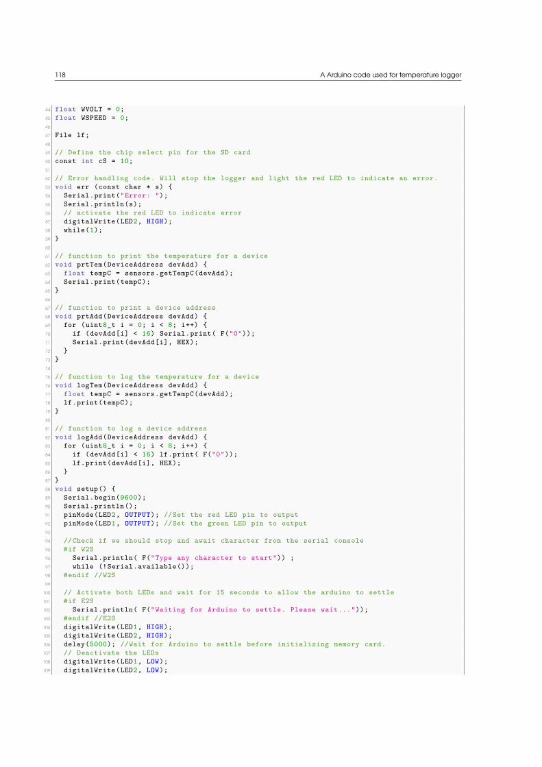
118 A Arduino code used for temperature logger
44 float WVOLT = 0;45 float WSPEED = 0;46
47 File lf;48
49 // Define the chip select pin for the SD card50 const int cS = 10;51
52 // Error handling code. Will stop the logger and light the red LED to indicate an error.53 void err (const char * s) 54 Serial.print("Error: ");55 Serial.println(s);56 // activate the red LED to indicate error57 digitalWrite(LED2, HIGH);58 while(1);59 60
61 // function to print the temperature for a device62 void prtTem(DeviceAddress devAdd) 63 float tempC = sensors.getTempC(devAdd);64 Serial.print(tempC);65 66
67 // function to print a device address68 void prtAdd(DeviceAddress devAdd) 69 for (uint8_t i = 0; i < 8; i++) 70 if (devAdd[i] < 16) Serial.print( F("0"));71 Serial.print(devAdd[i], HEX);72 73 74
75 // function to log the temperature for a device76 void logTem(DeviceAddress devAdd) 77 float tempC = sensors.getTempC(devAdd);78 lf.print(tempC);79 80
81 // function to log a device address82 void logAdd(DeviceAddress devAdd) 83 for (uint8_t i = 0; i < 8; i++) 84 if (devAdd[i] < 16) lf.print( F("0"));85 lf.print(devAdd[i], HEX);86 87 88 void setup() 89 Serial.begin(9600);90 Serial.println();91 pinMode(LED2, OUTPUT); //Set the red LED pin to output92 pinMode(LED1, OUTPUT); //Set the green LED pin to output93
94 //Check if we should stop and await character from the serial console95 #if W2S96 Serial.println( F("Type any character to start")) ;97 while (!Serial.available());98 #endif //W2S99
100 // Activate both LEDs and wait for 15 seconds to allow the arduino to settle101 #if E2S102 Serial.println( F("Waiting for Arduino to settle. Please wait..."));103 #endif //E2S104 digitalWrite(LED1, HIGH);105 digitalWrite(LED2, HIGH);106 delay(5000); //Wait for Arduino to settle before initializing memory card.107 // Deactivate the LEDs108 digitalWrite(LED1, LOW);109 digitalWrite(LED2, LOW);

A Arduino code used for temperature logger 119
110 Serial.println();111 //check if the SD card is present and can be initialized112 #if E2S113 Serial.print( F("Initializing SD card... "));114 #endif //E2S115 pinMode(cS, OUTPUT); // Set the pin used for the SD card to output116 if (!SD.begin(cS)) 117 err("Card failed or is not present!");118 119 #if E2S120 Serial.println( F("SD card initialized."));121 #endif //E2S122
123 //Create a new file to use for logging data124 char fn[] = "LOGGER00.CSV";125 for (uint8_t i = 0; i < 100; i++) 126 fn[6] = i/10 + '0';127 fn[7] = i%10 + '0';128 if (!SD.exists(fn)) 129 //Only open a new file if it does not already exist130 lf = SD.open(fn, FILE_WRITE);131 break; // Leave the loop132 133 134
135 if (! lf) 136 err( "Could not create file on SD card.");137 138
139 //Connect to the RTC module140 Wire.begin();141 if (! RTC.isrunning()) 142 Serial.println( F("RTC is NOT running!"));143 144 if (!RTC.begin()) 145 lf.println( F("RTC failed!"));146 err("RTC failed!");147 #if E2S148 Serial.println( F("RTC failed!"));149 #endif //E2S150 151 // to re-adjust the RTC clock, uncomment the line below.152 // RTC.adjust(DateTime(__DATE__, __TIME__));153
154
155 // Log information in lf156 lf.println( F("millis,stamp,Date-Time,AmbientT,AmbientH,WindSensorVolt,WindSensorSpeed,
Sensor1,Sensor2,Sensor3,Sensor4,Sensor5,Sensor6,Sensor7,Sensor8,Sensor9,Sensor10,Sensor11,Sensor12,Sensor13,Sensor14,Sensor15,Sensor16,Sensor17,Sensor18"));
157
158 //Start DHT sensor159 dht.begin();160 #if E2S161 Serial.print( F("Logging data to: "));162 Serial.println(fn);163 Serial.println( F("millis,stamp"));164 #endif //E2S165 #if L2S166 Serial.print( F("Date-Time,AmbientT,AmbientH,WindSensorVolt,WindSensorSpeed,Sensor1,
Sensor2,Sensor3,Sensor4,Sensor5,Sensor6,Sensor7,Sensor8,Sensor9,Sensor10,Sensor11,Sensor12,Sensor13,Sensor14,Sensor15,Sensor16,Sensor17,Sensor18"));
167 Serial.println();168 #endif //E2S169 float ambh = dht.readHumidity();170 float ambt = dht.readTemperature();171 if (isnan(ambh) || isnan(ambt))

120 A Arduino code used for temperature logger
172 err("Failed to read from DHT sensor!");173 return;174 175
176 //Setup D18B20 temperature sensors177 sensors.begin();178 DevCnt = sensors.getDeviceCount();179 #if E2S180 Serial.print( F("Locating D18B20 devices on bus... "));181 #endif //E2S182 if (DevCnt > 0) 183 #if E2S184 Serial.print( F("Found "));185 Serial.print(DevCnt, DEC);186 Serial.print( F(" devices."));187 Serial.println();188 #endif //E2S189
190 // Log serial numbers of the temperature sensors to the CSV file for future reference.191 lf.print( F("SERIAL ,NUMBERS ,FOR ,SENSORS ,FOLLOWS ,"));192 #if L2S193 Serial.print( F("SERIAL NUMBERS ,FOR SENSORS ,FOLLOWS ,"));194 #endif //L2S195 for (int i=0;i<DevCnt; i++) 196 if (sensors.getAddress(tmpDevAdd, i)) 197 logAdd(tmpDevAdd);198 lf.print(F(","));199 sensors.setResolution(tmpDevAdd, TEMP_PRE);200 #if L2S201 prtAdd(tmpDevAdd);202 Serial.print( F(","));203 #endif //L2S204 #if E2S205 Serial.print( F("Found device "));206 Serial.print(i, DEC);207 Serial.print( F(" with address: "));208 prtAdd(tmpDevAdd);209 Serial.println();210 Serial.print( F("Setting resolution to "));211 Serial.println(TEMP_PRE, DEC);212 Serial.print( F("Confirmed sensor resolution: "));213 Serial.print(sensors.getResolution(tmpDevAdd), DEC);214 Serial.println();215 #endif //E2S216 217 else 218 Serial.print( F("Found ghost device at "));219 Serial.print(i, DEC);220 Serial.print( F(" but could not detect address. Check power and wires"));221 222 223 lf.println();224 #if L2S225 Serial.println();226 #endif //L2S227 228 else 229 err("Did not find any temperature sensors, check the connections.");230 231
232
233 234
235 // Start logging loop236 void loop() 237 int cd = 0;

A Arduino code used for temperature logger 121
238 while (LOG_I-767 > cd) 239 digitalWrite(LED1, HIGH);240 delay(250);241 digitalWrite(LED1, LOW);242 delay(250);243 cd = cd + 500;244 245 //Delay for the logging interval246 //delay((LOG_I -1) - (millis() % LOG_I));247 DateTime now = RTC.now();248 digitalWrite(LED1, HIGH); //activate the green LED to indicate that logging is active249 // log milliseconds seens starting250 uint32_t m = millis();251 lf.print(m);252 lf.print(F(","));253 #if E2S254 Serial.print(m); // milliseconds since start255 Serial.print(F(","));256 #endif E2S257
258 //Fetch the time259 now = RTC.now();260 // log time261 lf.print(now.unixtime()); // seconds since 1/1/1970262 lf.print(F(","));263 lf.print('"');264 lf.print(now.year(), DEC);265 lf.print(F("/"));266 lf.print(now.month(), DEC);267 lf.print(F("/"));268 lf.print(now.day(), DEC);269 lf.print(F(" "));270 lf.print(now.hour(), DEC);271 lf.print(F(":"));272 lf.print(now.minute(), DEC);273 lf.print(F(":"));274 lf.print(now.second(), DEC);275 lf.print('"');276 #if E2S277 Serial.print(now.unixtime()); // seconds since 1/1/1970278 Serial.print(F(","));279 #endif //E2S280 #if L2S281 Serial.print('"');282 Serial.print(now.year(), DEC);283 Serial.print(F("/"));284 Serial.print(now.month(), DEC);285 Serial.print(F("/"));286 Serial.print(now.day(), DEC);287 Serial.print(F(" "));288 Serial.print(now.hour(), DEC);289 Serial.print(F(":"));290 Serial.print(now.minute(), DEC);291 Serial.print(F(":"));292 Serial.print(now.second(), DEC);293 Serial.print('"');294 #endif //L2S295 // Read ambient temperature and humidity from the DHT22296 // Reading temperature or humidity takes about 250 milliseconds!297 // Sensor readings may also be up to 2 seconds 'old' (its a very slow sensor)298 float ambh = dht.readHumidity();299 // Read temperature as Celsius (the default)300 float ambt = dht.readTemperature();301 // Check if any reads failed and exit early (to try again).302 if (isnan(ambh) || isnan(ambt)) 303 // err("Failed to read from DHT sensor!");

122 A Arduino code used for temperature logger
304 return;305 306 lf.print(F(","));307 lf.print(ambt);308 lf.print(F(","));309 lf.print(ambh);310 #if L2S311 Serial.print(F(","));312 Serial.print(ambt);313 Serial.print(F(","));314 Serial.print(ambh);315 #endif //L2S316
317 // Record wind speed318 WVAL = analogRead(W_P);319 if (WVAL > 0) 320 WVOLT = 0.005 + (WVAL * 2.5 * 0.004873046875);321 322 else 323 WVOLT = (WVAL * 2.5 * 0.004873046875);324 325
326 if (WVAL > 0) 327 WSPEED = 0.9 + (WVOLT * 4.2806);328 329 else 330 WSPEED = 0;331 332 lf.print(",");333 lf.print(WVOLT);334 lf.print(",");335 lf.print(WSPEED);336 #if L2S337 Serial.print(",");338 Serial.print(WVOLT);339 Serial.print(",");340 Serial.print(WSPEED);341 #endif //L2S342
343 // Read data from the D18B20 temperature sensors344 //Serial.print( F("Requesting temperatures from D18B20 devices... "));345 sensors.requestTemperatures(); // Send command to get temperatures346 //Serial.println( F("DONE"));347 // Loop through each device, print out temperature data348 for(int i=0;i<DevCnt; i++) 349 // Search the wire for address350 if(sensors.getAddress(tmpDevAdd, i)) 351 // Output the device ID352 lf.print(F(","));353 logTem(tmpDevAdd);354 #if L2S355 Serial.print(F(","));356 prtTem(tmpDevAdd);357 #endif L2S358 359 //else ghost device! Check your power requirements and cabling360 361 lf.println();362 #if L2S363 Serial.println();364 #endif //L2S365
366 digitalWrite(LED1, LOW);367
368 // Write data to SD card369 if ((millis() - syncTime) < SYNC_I) return;

A Arduino code used for temperature logger 123
370 syncTime = millis();371 //flash LED to show that the data is written to the SD card372 digitalWrite(LED2, HIGH);373 lf.flush();374 digitalWrite(LED2, LOW);375
.

124

APPENDIX BCode used for calculations
The following code is based on the work performed by (Kvamme, 2014). The code provided by (Kvamme,2014) only contained calculations for uninsulated and insulated pipes, and only the Churchill-Bernsteincorrelation. The revised code is rewritten in Python to enable open-source and free use contains allheat transfer correlations presented in section 2.2.2 for forced flow over a cylinder. To use this code,the free Python distribution Anaconda can be used.
1 ## Code for calculating heat loss from cylinders2 ## Written by Bjarte Odin Kvamme3 ## Licensed as beerware. If you in some parallell universe was to meet me, buy me a beer.
Otherwise, use freely, but give credit as needed.4
5 ## Import required packages6 import numpy as np7 import scipy as sp8 import matplotlib as mpl9 import matplotlib.pyplot as plt
10
11 ##12
13 from numpy import *14 from math import pi15 import scipy.linalg16 from datetime import datetime17 import xlsxwriter18
19 ## Define variables20 V_infty = [0.05, 5, 10, 15] # Wind Speed values in m/s, comma delimited21 TiC = [10] # Initial temperature of pipe, in degrees Celsius, comma
delimited22 TeC = [-20] # External temperature, in degrees Celsius, comma delimited23 D_tab = [0.025, 0.050, 0.1, 0.5, 1.0] # Table of pipe outer diameter24 t_w = 0.002 # Wall thickness of pipe25 p_atm = 103.1 # Air pressure, in kilopascal (kPa) obtained from Incropera
et al., 2006.26 Tc = 272.15 # Desired temperature of ice27
28 # Create inital array to store the results obtained29 results = []30 results.append([])31 row = 0 # Initial loop counter value32
33 ## Constants34 # Properties of pipe35 D_i = 0.046 # Inner diameter of pipe (m)36 D_o = 0.050 # Outer diameter of pipe (m)37 t_ice = 0.005 # Thickness of external ice layer (m)38 k_pipe = 43 # Thermal conductivity of carbon steel pipe (W/(m K))39
40 # Properties of insulation41 t_ins = [0, 0.005, 0.01, 0.05] # Thickness of insulation (m)42 k_ins = 0.033 # Thermal conductivity of insulation (W/(m K))43
44 # Properties of air45 #Pr_air = 0.714 # Prandt number for air at 10C

126 B Code used for calculations
46 #k_air = 0.02265 # Thermal Conductivity of air (W/(m K))47 #v_air = 13.3e-6 # Kinematic viscosity of air (m2/s)48 #rho_air = 1.3163 # Density of air at -5C (kg/m3)49 #mu_air = 1.76e-5 # Dynamic viscosity of air (kg/m s)50 R_air = 0.287 # kJ / kg K obtained from Incropera et al., 2006.51
52 # Properties of water53 cp_w = 4217 # Specific heat of water at 5C (J/(Kg K)) obtained from
Incropera et al., 2006.54 Tf_w = 273.15 # Freezing temperature of water (0C) obtained from
Incropera et al., 2006.55 h_w = 1000 # Heat transfer co-efficient of water (W/(m2 K))56 rho_w = 1000 # Density of water at 0C (kg/m3) obtained from Incropera
et al., 2006.57 hfs_w = 333.7 # Latent heat of fusion for water (J/g) obtained from
Incropera et al., 2006.58
59 # Properties of ice60 k_ice = 1.88 # Thermal conductivity of ice at 0C (W/(m K)) obtained from
Incropera et al., 2006.61 rho_ice = 920 # Density of ice at 0C (kg/m3) obtained from Incropera et
al., 2006.62 cp_ice = 2.04063
64 # Properties of heat tracing65 # ql_ht = 50 # Applied heat (W/m) from heat tracing66
67 # All functions below assume steady-state conditions.68
69 # Thermodynamic properties of air, obtained from Incropera et al., 2006.70 alpha_air_table = '100': 2.54E-6, '150': 5.84E-6, '200': 10.3E-6, '250': 15.9E-6, '300':
22.5E-6, '350': 29.9E-6, '400': 38.3E-6, '450': 47.2E-671 k_air_table = '100': 9.34E-3, '150': 13.8E-3, '200': 18.1E-3, '250': 22.3E-3, '300': 26.3E
-3, '350': 30.0E-3, '400': 33.8E-3, '450': 37.3E-372 mu_air_table = '100': 71.1E-7, '150': 103.4E-7, '200': 132.5E-7, '250': 159.6E-7, '300':
184.6E-7, '350': 208.2E-7, '400': 230.1E-7, '450': 250.7E-773 cp_air_table = '100': 1.032, '150': 1.012, '200': 1.007, '250': 1.006, '300': 1.007, '350':
1.009, '400': 1.014, '450': 1.02174 nu_air_table = '100': 2.00E-6, '150': 4.426E-6, '200': 7.590E-6, '250': 11.44E-6, '300':
15.89E-6, '350': 20.92E-6, '400': 26.41E-6, '450': 32.39E-675 Pr_air_table = '100': 0.786, '150': 0.758, '200': 0.737, '250': 0.720, '300': 0.707, '350':
0.700, '400': 0.690, '450': 0.68676 Rho_air_table = '100': 3.5562, '150': 2.3364, '200': 1.7458, '250': 1.3947, '300': 1.1614, '
350': 0.9950, '400': 0.87711, '450': 0.774077
78 # Thermodynamic properties of water, obtained from Incropera et al., 2006.79 cp_w_table = '273.15': 4.217, '275': 4.211, '280': 4.198, '285': 4.189, '290': 4.184, '295':
4.181, '300': 4.179, '305': 4.178, '310': 4.178, '315': 4.179, '320': 4.180, '325':4.182, '330': 4.184, '335': 4.186, '340': 4.188, '345': 4.191
80
81 # Hilpert correlation constants82 Hilpert_C = '1-4': 0.891, '4-40': 0.821, '40-4000': 0.615, '4000-40000': 0.174, '
40000-400000': 0.023983 Hilpert_m = '1-4': 0.330, '4-40': 0.385, '40-4000': 0.466, '4000-40000': 0.618, '
40000-400000': 0.80584
85 # Updated Hilpert correlation constants86 UpdatedHilpert_C = '0.4-4': 0.989, '4-40': 0.911, '40-4000': 0.683, '4000-40000': 0.193, '
40000-400000': 0.02787 UpdatedHilpert_m = '0.4-4': 0.330, '4-40': 0.385, '40-4000': 0.466, '4000-40000': 0.618, '
40000-400000': 0.80588
89 # Updated Hilpert correlation constants, Fand & Keswani (1973)90 FandKeswani_C = '1-4': 0.875, '4-40': 0.785, '40-4000': 0.590, '4000-40000': 0.154, '
40000-400000': 0.024791 FandKeswani_m = '1-4': 0.313, '4-40': 0.388, '40-4000': 0.467, '4000-40000': 0.627, '
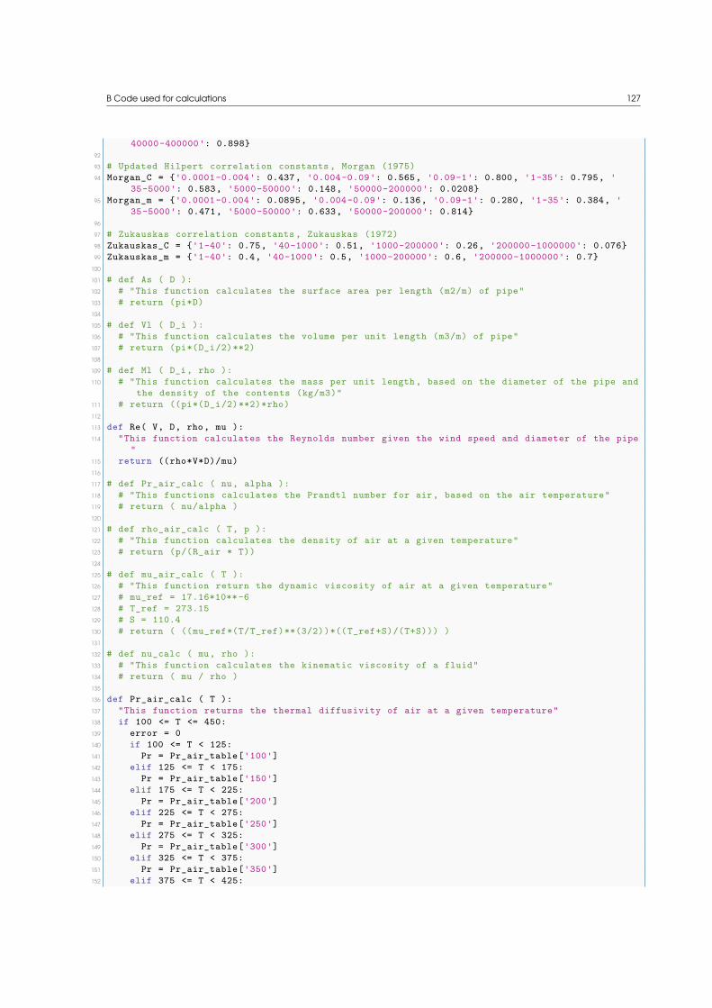
B Code used for calculations 127
40000-400000': 0.89892
93 # Updated Hilpert correlation constants, Morgan (1975)94 Morgan_C = '0.0001-0.004': 0.437, '0.004-0.09': 0.565, '0.09-1': 0.800, '1-35': 0.795, '
35-5000': 0.583, '5000-50000': 0.148, '50000-200000': 0.020895 Morgan_m = '0.0001-0.004': 0.0895, '0.004-0.09': 0.136, '0.09-1': 0.280, '1-35': 0.384, '
35-5000': 0.471, '5000-50000': 0.633, '50000-200000': 0.81496
97 # Zukauskas correlation constants, Zukauskas (1972)98 Zukauskas_C = '1-40': 0.75, '40-1000': 0.51, '1000-200000': 0.26, '200000-1000000': 0.07699 Zukauskas_m = '1-40': 0.4, '40-1000': 0.5, '1000-200000': 0.6, '200000-1000000': 0.7
100
101 # def As ( D ):102 # "This function calculates the surface area per length (m2/m) of pipe"103 # return (pi*D)104
105 # def Vl ( D_i ):106 # "This function calculates the volume per unit length (m3/m) of pipe"107 # return (pi*(D_i/2)**2)108
109 # def Ml ( D_i, rho ):110 # "This function calculates the mass per unit length, based on the diameter of the pipe and
the density of the contents (kg/m3)"111 # return ((pi*(D_i/2)**2)*rho)112
113 def Re( V, D, rho, mu ):114 "This function calculates the Reynolds number given the wind speed and diameter of the pipe
"115 return ((rho*V*D)/mu)116
117 # def Pr_air_calc ( nu, alpha ):118 # "This functions calculates the Prandtl number for air, based on the air temperature"119 # return ( nu/alpha )120
121 # def rho_air_calc ( T, p ):122 # "This function calculates the density of air at a given temperature"123 # return (p/(R_air * T))124
125 # def mu_air_calc ( T ):126 # "This function return the dynamic viscosity of air at a given temperature"127 # mu_ref = 17.16*10**-6128 # T_ref = 273.15129 # S = 110.4130 # return ( ((mu_ref*(T/T_ref)**(3/2))*((T_ref+S)/(T+S))) )131
132 # def nu_calc ( mu, rho ):133 # "This function calculates the kinematic viscosity of a fluid"134 # return ( mu / rho )135
136 def Pr_air_calc ( T ):137 "This function returns the thermal diffusivity of air at a given temperature"138 if 100 <= T <= 450:139 error = 0140 if 100 <= T < 125:141 Pr = Pr_air_table['100']142 elif 125 <= T < 175:143 Pr = Pr_air_table['150']144 elif 175 <= T < 225:145 Pr = Pr_air_table['200']146 elif 225 <= T < 275:147 Pr = Pr_air_table['250']148 elif 275 <= T < 325:149 Pr = Pr_air_table['300']150 elif 325 <= T < 375:151 Pr = Pr_air_table['350']152 elif 375 <= T < 425:

128 B Code used for calculations
153 Pr = Pr_air_table['400']154 elif 425 <= T <= 450:155 Pr = Pr_air_table['450']156 if error == 0:157 return ( Pr )158 else:159 return ('N/A')160
161 def cp_w_calc ( T ):162 "This function returns the thermal diffusivity of air at a given temperature"163 if 273.15 <= T <= 350:164 error = 0165 if 273.15 <= T < 275:166 cp_w = cp_w_table['273.15']167 elif 275 <= T < 280:168 cp_w = cp_w_table['275']169 elif 280 <= T < 285:170 cp_w = cp_w_table['280']171 elif 285 <= T < 290:172 cp_w = cp_w_table['285']173 elif 290 <= T < 295:174 cp_w = cp_w_table['290']175 elif 295 <= T < 300:176 cp_w = cp_w_table['295']177 elif 300 <= T < 305:178 cp_w = cp_w_table['300']179 elif 305 <= T < 310:180 cp_w = cp_w_table['305']181 elif 310 <= T < 315:182 cp_w = cp_w_table['310']183 elif 315 <= T < 320:184 cp_w = cp_w_table['315']185 elif 320 <= T < 325:186 cp_w = cp_w_table['320']187 elif 325 <= T < 330:188 cp_w = cp_w_table['325']189 elif 330 <= T < 335:190 cp_w = cp_w_table['330']191 elif 335 <= T < 340:192 cp_w = cp_w_table['335']193 elif 340 <= T < 345:194 cp_w = cp_w_table['340']195 elif 345 <= T <= 350:196 cp_w = cp_w_table['345']197 if error == 0:198 return ( cp_w )199 else:200 return ('N/A')201
202 def Rho_air_calc ( T ):203 "This function returns the thermal diffusivity of air at a given temperature"204 if 100 <= T <= 450:205 error = 0206 if 100 <= T < 125:207 Rho = Rho_air_table['100']208 elif 125 <= T < 175:209 Rho = Rho_air_table['150']210 elif 175 <= T < 225:211 Rho = Rho_air_table['200']212 elif 225 <= T < 275:213 Rho = Rho_air_table['250']214 elif 275 <= T < 325:215 Rho = Rho_air_table['300']216 elif 325 <= T < 375:217 Rho = Rho_air_table['350']218 elif 375 <= T < 425:

B Code used for calculations 129
219 Rho = Rho_air_table['400']220 elif 425 <= T <= 450:221 Rho = Rho_air_table['450']222 if error == 0:223 return ( Rho )224 else:225 return ('N/A')226
227 def nu_air_calc ( T ):228 "This function returns the thermal diffusivity of air at a given temperature"229 if 100 <= T <= 450:230 error = 0231 if 100 <= T < 125:232 nu = nu_air_table['100']233 elif 125 <= T < 175:234 nu = nu_air_table['150']235 elif 175 <= T < 225:236 nu = nu_air_table['200']237 elif 225 <= T < 275:238 nu = nu_air_table['250']239 elif 275 <= T < 325:240 nu = nu_air_table['300']241 elif 325 <= T < 375:242 nu = nu_air_table['350']243 elif 375 <= T < 425:244 nu = nu_air_table['400']245 elif 425 <= T <= 450:246 nu = nu_air_table['450']247 if error == 0:248 return ( nu )249 else:250 return ('N/A')251
252 def mu_air_calc ( T ):253 "This function returns the thermal diffusivity of air at a given temperature"254 if 100 <= T <= 450:255 error = 0256 if 100 <= T < 125:257 mu = mu_air_table['100']258 elif 125 <= T < 175:259 mu = mu_air_table['150']260 elif 175 <= T < 225:261 mu = mu_air_table['200']262 elif 225 <= T < 275:263 mu = mu_air_table['250']264 elif 275 <= T < 325:265 mu = mu_air_table['300']266 elif 325 <= T < 375:267 mu = mu_air_table['350']268 elif 375 <= T < 425:269 mu = mu_air_table['400']270 elif 425 <= T <= 450:271 mu = mu_air_table['450']272 if error == 0:273 return ( mu )274 else:275 return ('N/A')276
277 def k_air_calc ( T ):278 "This function returns the thermal conductivity of the air for a given temperature"279 if 100 <= T <= 450:280 error = 0281 if 100 <= T < 125:282 k = k_air_table['100']283 elif 125 <= T < 175:284 k = k_air_table['150']

130 B Code used for calculations
285 elif 175 <= T < 225:286 k = k_air_table['200']287 elif 225 <= T < 275:288 k = k_air_table['250']289 elif 275 <= T < 325:290 k = k_air_table['300']291 elif 325 <= T < 375:292 k = k_air_table['350']293 elif 375 <= T < 425:294 k = k_air_table['400']295 elif 425 <= T <= 450:296 k = k_air_table['450']297 if error == 0:298 return ( k )299 else:300 return ('N/A')301
302 def alpha_air_calc ( T ):303 "This function returns the thermal diffusivity of air at a given temperature"304 if 100 <= T <= 450:305 error = 0306 if 100 <= T < 125:307 alpha = alpha_air_table['100']308 elif 125 <= T < 175:309 alpha = alpha_air_table['150']310 elif 175 <= T < 225:311 alpha = alpha_air_table['200']312 elif 225 <= T < 275:313 alpha = alpha_air_table['250']314 elif 275 <= T < 325:315 alpha = alpha_air_table['300']316 elif 325 <= T < 375:317 alpha = alpha_air_table['350']318 elif 375 <= T < 425:319 alpha = alpha_air_table['400']320 elif 425 <= T <= 450:321 alpha = alpha_air_table['450']322 if error == 0:323 return ( alpha )324 else:325 return ('N/A')326
327 def T_film ( Ti, Te ):328 "This function calculates the film temperature, to be used for fluid properties"329 return ((Ti + Te)/2)330
331 def Nu_CB ( Re, Pr ):332 "This function calculates the Nusselts number using the Churchill-Bernstein correlation"333 if Re*Pr >= 0.2:334 error = 0335 else:336 error = 1337 if error == 0:338 return 0.3+(0.62*(Re**0.5)*Pr**(1/3)/((1+(0.4/Pr)**(2/3))**(1/4)))*(1+(Re/282000)**(5/8))
**(4/5)339 else:340 return ('N/A')341 342 def Nu_Hilpert ( Re, Pr, Corr ):343 if Corr == 'Original':344 if 1 <= Re <= 400000 and Pr >= 0.7:345 error = 0346 if 1 <= Re <= 4:347 C = Hilpert_C['1-4']348 m = Hilpert_m['1-4']349 elif 4 < Re <= 40:
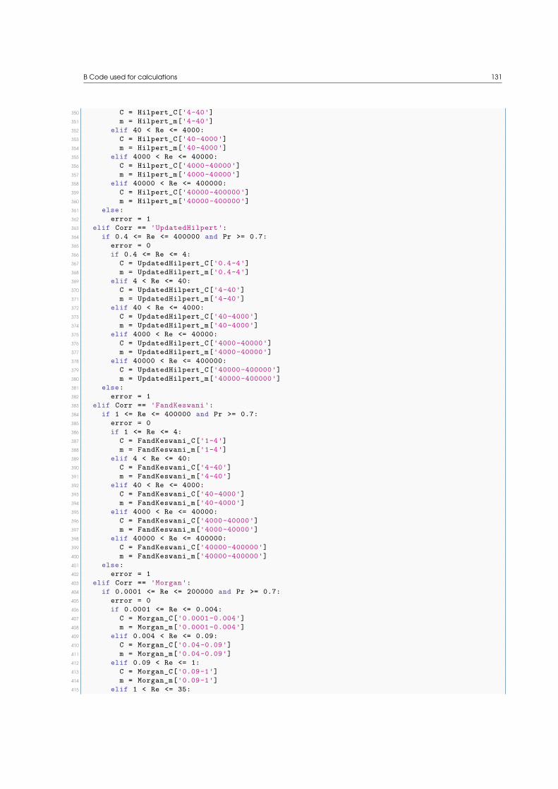
B Code used for calculations 131
350 C = Hilpert_C['4-40']351 m = Hilpert_m['4-40']352 elif 40 < Re <= 4000:353 C = Hilpert_C['40-4000']354 m = Hilpert_m['40-4000']355 elif 4000 < Re <= 40000:356 C = Hilpert_C['4000-40000']357 m = Hilpert_m['4000-40000']358 elif 40000 < Re <= 400000:359 C = Hilpert_C['40000-400000']360 m = Hilpert_m['40000-400000']361 else:362 error = 1363 elif Corr == 'UpdatedHilpert':364 if 0.4 <= Re <= 400000 and Pr >= 0.7:365 error = 0366 if 0.4 <= Re <= 4:367 C = UpdatedHilpert_C['0.4-4']368 m = UpdatedHilpert_m['0.4-4']369 elif 4 < Re <= 40:370 C = UpdatedHilpert_C['4-40']371 m = UpdatedHilpert_m['4-40']372 elif 40 < Re <= 4000:373 C = UpdatedHilpert_C['40-4000']374 m = UpdatedHilpert_m['40-4000']375 elif 4000 < Re <= 40000:376 C = UpdatedHilpert_C['4000-40000']377 m = UpdatedHilpert_m['4000-40000']378 elif 40000 < Re <= 400000:379 C = UpdatedHilpert_C['40000-400000']380 m = UpdatedHilpert_m['40000-400000']381 else:382 error = 1383 elif Corr == 'FandKeswani':384 if 1 <= Re <= 400000 and Pr >= 0.7:385 error = 0386 if 1 <= Re <= 4:387 C = FandKeswani_C['1-4']388 m = FandKeswani_m['1-4']389 elif 4 < Re <= 40:390 C = FandKeswani_C['4-40']391 m = FandKeswani_m['4-40']392 elif 40 < Re <= 4000:393 C = FandKeswani_C['40-4000']394 m = FandKeswani_m['40-4000']395 elif 4000 < Re <= 40000:396 C = FandKeswani_C['4000-40000']397 m = FandKeswani_m['4000-40000']398 elif 40000 < Re <= 400000:399 C = FandKeswani_C['40000-400000']400 m = FandKeswani_m['40000-400000']401 else:402 error = 1403 elif Corr == 'Morgan':404 if 0.0001 <= Re <= 200000 and Pr >= 0.7:405 error = 0406 if 0.0001 <= Re <= 0.004:407 C = Morgan_C['0.0001-0.004']408 m = Morgan_m['0.0001-0.004']409 elif 0.004 < Re <= 0.09:410 C = Morgan_C['0.04-0.09']411 m = Morgan_m['0.04-0.09']412 elif 0.09 < Re <= 1:413 C = Morgan_C['0.09-1']414 m = Morgan_m['0.09-1']415 elif 1 < Re <= 35:

132 B Code used for calculations
416 C = Morgan_C['1-35']417 m = Morgan_m['1-35']418 elif 35 < Re <= 5000:419 C = Morgan_C['35-5000']420 m = Morgan_m['35-5000']421 elif 5000 < Re <= 50000:422 C = Morgan_C['5000-50000']423 m = Morgan_m['5000-50000']424 elif 50000 < Re <= 200000:425 C = Morgan_C['50000-200000']426 m = Morgan_m['50000-200000']427 else:428 error = 1429 if error == 0:430 return (C*(Re**(m))*Pr**(1/3))431 else:432 return ('N/A')433
434 def Nu_Zukauskas( Re, Pr, Prs ):435 if 0.7 <= Pr <= 500 and 1 <= Re <= 1000000:436 error = 0437 if Pr < 10:438 n = 0.37439 elif Pr >= 10:440 n = 0.36441 if 1 <= Re <= 40:442 C = Zukauskas_C['1-40']443 m = Zukauskas_m['1-40']444 elif 40 < Re <= 1000:445 C = Zukauskas_C['40-1000']446 m = Zukauskas_m['40-1000']447 elif 1000 < Re <= 200000:448 C = Zukauskas_C['1000-200000']449 m = Zukauskas_m['1000-200000']450 elif 200000 < Re <= 1000000:451 C = Zukauskas_C['200000-1000000']452 m = Zukauskas_m['200000-1000000']453 else: error = 1454 if error == 0:455 return (C*(Re**(m))*Pr**(n)*(Pr/Prs)**(1/4))456 else:457 return ('N/A')458
459 def Nu_Whittaker ( Re, Pr, Ti, Te ):460 mu_b = mu_air_calc(Te)461 mu_s = mu_air_calc(Ti)462 if 1 <= Re <= 100000 and 0.67 <= Pr <= 300:463 error = 0464 else:465 error = 1466 if error == 0:467 return ((0.5*(Re**(1/2))+0.06*(Re**(2/3)))*(Pr**(0.4))*((mu_b/mu_s)**(1/4)))468 else:469 return ('N/A')470
471 def h_conv( Nu, k, D_o ):472 "This function calculates the convective heat transfer co-efficient of an external flow
over a pipe"473 return ((Nu*k)/D_o)474
475 def U0(h_external, k_pipe, D_i, D_o ):476 print(h_external)477 print(k_pipe)478 print(D_i)479 print(D_o)480 print(((D_o*math.log(D_o/D_i))/(2*k_pipe)))

B Code used for calculations 133
481 print(1/h_external)482 "This function calculates the overall heat transfer co-efficient of an uninsulated pipe.
h_internal is the internal heat transfer co-efficient, h_external is the external heattransfer co-efficient, kp is the thermal conductivity of the pipe, ID is the internaldiameter of the pipe, OD is the outer diameter of the pipe."
483 return (1/(((D_o*math.log(D_o/D_i))/(2*k_pipe))+(1/h_external)))484
485 def U1(h_external, k_pipe, k_ins, D_i, D_o, t_ins ):486 D_o_ins = D_o + 2*t_ins487 "This function calculates the overall heat transfer co-efficient of an insulated pipe.
h_internal is the internal heat transfer co-efficient, h_external is the external heattransfer co-efficient, kp is the thermal conductivity of the pipe, k_ins is the thermalconductivity of the insulation, ID is the internal diameter of the pipe, OD is the outerdiameter of the pipe and ti is the thickness of the insulation"
488 #return (1/(((D_o_ins*math.log(D_o/D_i))/(2*k_pipe))+((D_o_ins*math.log(D_o_ins/D_o))/(2*k_ins))+(1/h_external)))
489 return (1/(((D_o_ins*math.log(D_o_ins/D_o))/(2*k_ins))+(1/h_external)))490
491 def U2(h_external, k_pipe, k_ins, k_ice, D_i, D_o, t_ins, t_ice ):492 D_o_ins = D_o + 2*t_ins493 D_o_ins_ice = D_o_ins + 2*t_ice494 "This function calculates the overall heat transfer co-efficient of an insulated pipe with
ice. h_internal is the internal heat transfer co-efficient, h_external is the externalheat transfer co-efficient, kp is the thermal conductivity of the pipe, k_ins is thethermal conductivity of the insulation, k_ice is the thermal conductivity of ice, ID isthe internal diameter of the pipe, OD is the outer diameter of the pipe, ti is thethickness of the insulation and tice is the thickness of the ice glazing."
495 return (1/(((D_o_ins_ice*math.log(D_o/D_i))/(2*k_pipe))+((D_o_ins_ice*math.log(D_o_ins/D_o))/(2*k_ins))+((D_o_ins_ice*math.log(D_o_ins_ice/D_o_ins))/(2*k_ice))+(1/h_external)))
496
497 # def ql( U, A, Ti, Te ):498 # "This function calculates the heat loss, or heat flux of a pipe in W/m"499 # return (U*A*(Ti-Te))500
501 # def tc( Ml, Ti, Te, ql ):502 # "This function calculates the required time (in seconds) to cool water inside a unit
length of pipe to freezing temperature (0degC)."503 # return ((cp_w*Ml*(Ti-Tf_w))/ql)504
505 # def tf_w( Ml, ql ):506 # "This function calculates the required time (in seconds) to freeze water inside a unit
length of pipe."507 # return ((hfs_w*Ml)/ql)508
509 def TimeToFreeze(h_external, rho_s, rho_l, Hf, c_s, c_l, k_s, Ti, Tamb, Tf, Tc, D, L):510 "This function calculates the time to freeze a cylinder filled with a liquid"511 h_l = Hf + (Ti-Tf)*c_l512 h_s = (Tf-Tc)*c_s513 deltaH = (rho_l*h_l)-(rho_s*h_s)514 Cs = (rho_s*c_s)515 Cl = (rho_l*c_l)516 Beta = (L/D)517 Bi = ((h_external*D)/k_s)518 Pk = ((Cl*(Ti-Tf))/deltaH)519 Ste = ((Cs*(Tf-Tamb))/deltaH)520 deltaT = ((Tf-Tamb)+((((Ti-Tf)**2)*(Cl/2)-(((Tf-Tc)**2)*(Cs/2)))/deltaH))521 U = (deltaT/(Tf-Tamb))522 P = (0.7306-(1.083*Pk)+Ste*((15.4*U)-15.43+(0.01329*(Ste/Bi))))523 R = (0.2079-0.2656*U*Ste)524 theta = (((deltaH*10**3)/deltaT)*(((P*D)/h_external)+((R*(D**2))/k_s)))525 phi = (2.32/(Beta**1.77))526 X = (phi/((Bi**1.34)+phi))527 E2 = ((X/Beta)+((1-X)*(0.5/(Beta**3.69))))528 E = (2+E2)529 theta_shape = ((theta/E)/3600)530 return (theta_shape)

134 B Code used for calculations
531
532
533 # Prepare spreadsheet for results534 workbook = xlsxwriter.Workbook('Results.xlsx')535 worksheet = workbook.add_worksheet()536 bold = workbook.add_format('bold': 1)537 merge_format = workbook.add_format(538 'bold': 1,539 'align': 'center',540 'valign': 'vcenter')541 #worksheet.set_column(1, 1, 15)542 worksheet.write(2, 0, 'Pipe OD', bold)543 worksheet.write(2, 1, 't_ins', bold)544 worksheet.write(2, 2, 'V_infty', bold)545 worksheet.write(2, 3, 'TiC', bold)546 worksheet.write(2, 4, 'TeC', bold)547 worksheet.write(2, 5, 'Re', bold)548 for g in range(0,3):549 g = 0550 label = ['Nu', 'h', 'U', 'ttf, h']551 for h in range(6,34):552 worksheet.write(2, h, label[g], bold)553 if g < 3:554 g += 1555 elif g == 3:556 g = 0557
558 # Merge headers559 worksheet.merge_range(1, 0, 1, 5, 'Common', merge_format)560 worksheet.merge_range(1, 6, 1, 9, 'Hilpert Correlation', merge_format)561 worksheet.merge_range(1, 10, 1, 13, 'Updated Hilpert', merge_format)562 worksheet.merge_range(1, 14, 1, 17, 'Fand & Keswani', merge_format)563 worksheet.merge_range(1, 18, 1, 21, 'Morgan', merge_format)564 worksheet.merge_range(1, 22, 1, 25, 'Zukauskas', merge_format)565 worksheet.merge_range(1, 26, 1, 29, 'Whitaker', merge_format)566 worksheet.merge_range(1, 30, 1, 33, 'Churchill-Bernstein', merge_format)567
568
569 counter_row = 3570 counter_column = 0571 # Starting main calculation loop572
573 # Calculating fixed variables574 # Ml_temp = Ml(D_i, rho_w)575 # D_o_ice = D_o+2*t_ice576 # D_o_ins = D_o+2*t_ins577 # D_o_ins_ice = D_o_ins+2*t_ice578
579 for i in range(len(V_infty)):580 print('Calculating for a wind speed of', V_infty[i], ' m/s')581 for j in range(len(TiC)):582 Ti = TiC[j]+273.15583 print('Calculating for an internal temperature of', Ti, ' degC')584 for k in range(len(TeC)):585 Te = TeC[k]+273.15586 T_film_temp = T_film(Ti, Te)587 # Pr_air_temp = Pr_air_calc( nu_calc(mu_air_calc(T_film(Ti, Te))),alpha_air_calc(T_film
(Ti, Te)))588 Pr_air_inf = Pr_air_calc(Te)589 Pr_air_film = Pr_air_calc(T_film_temp)590 Pr_air_surf = Pr_air_calc(Ti)591 print('Calculating for an external temperature of ', Te, ' degC')592 for l in range(len(D_tab)):593 print('Calculating for an Pipe OD of ', D_tab[l], ' m')594 for m in range(len(t_ins)):595 print('Calculating for a insulation thickness of ', t_ins[m], ' m')

B Code used for calculations 135
596 D_o = D_tab[l]+2*t_ins[m]597 D_i = D_tab[l]-2*t_w598 Re_temp = Re(V_infty[i], D_o, Rho_air_calc(T_film_temp), mu_air_calc(T_film_temp))599 Re_amb = Re(V_infty[i], D_o, Rho_air_calc(Te), mu_air_calc(Te))600 worksheet.write(counter_row, counter_column, D_tab[l])601 counter_column += 1602 worksheet.write(counter_row, counter_column, t_ins[m])603 counter_column += 1604 worksheet.write(counter_row, counter_column, V_infty[i])605 counter_column += 1606 worksheet.write(counter_row, counter_column, TiC[j])607 counter_column += 1608 worksheet.write(counter_row, counter_column, TeC[k])609 counter_column += 1610 worksheet.write(counter_row, counter_column, Re_temp)611 counter_column += 1612 for n in range(0,4):613 # Calculate heat loss for uninsulated pipe using Hilpert614 Corr = ['Original', 'UpdatedHilpert', 'FandKeswani', 'Morgan']615 print('Calculating Hilpert', Corr[n])616 Nu_temp = Nu_Hilpert(Re_temp, Pr_air_film, Corr[n])617 if Nu_temp == 'N/A':618 h_temp = 'N/A'619 U_temp = 'N/A'620 ttf = 'N/A'621 else:622 k_air_temp = k_air_calc (T_film_temp)623 h_temp = h_conv(Nu_temp, k_air_temp, D_o)624 if t_ins[m] == 0:625 U_temp = U0(h_temp, k_pipe, D_i, D_tab[l])626 elif t_ins[m] > 0:627 U_temp = U1(h_temp, k_pipe, k_ins, D_i, D_tab[l], t_ins[m])628 ttf = TimeToFreeze(U_temp, rho_ice, rho_w, hfs_w, cp_ice, cp_w_calc(Ti), k_ice,
Ti, Te, Tf_w, Tc, D_i, 1)629 worksheet.write(counter_row, counter_column, Nu_temp) # Write Nusselts number to
spreadsheet630 counter_column += 1631 worksheet.write(counter_row, counter_column, h_temp) # Write convective heat
transfer co-efficient to spreadsheet632 counter_column += 1633 worksheet.write(counter_row, counter_column, U_temp) # Write overall heat
transfer co-efficient to spreadsheet634 counter_column += 1635 worksheet.write(counter_row, counter_column, ttf) # Write time to freeze to
spreadsheet636 counter_column += 1637 # Calculate heat loss for uninsulated pipe using Zukauskas638 print('Calculating Zukauskas')639 Nu_temp = Nu_Zukauskas(Re_amb, Pr_air_inf, Pr_air_surf)640 if Nu_temp == 'N/A':641 h_temp = 'N/A'642 U_temp = 'N/A'643 ttf = 'N/A'644 else:645 k_air_temp = k_air_calc (T_film_temp)646 h_temp = h_conv(Nu_temp, k_air_temp, D_o)647 if t_ins[m] == 0:648 U_temp = U0(h_temp, k_pipe, D_i, D_tab[l])649 elif t_ins[m] > 0:650 U_temp = U1(h_temp, k_pipe, k_ins, D_i, D_tab[l], t_ins[m])651 ttf = TimeToFreeze(U_temp, rho_ice, rho_w, hfs_w, cp_ice, cp_w_calc(Ti), k_ice,
Ti, Te, Tf_w, Tc, D_i, 1)652 worksheet.write(counter_row, counter_column, Nu_temp) # Write Nusselts number to
spreadsheet653 counter_column += 1654 worksheet.write(counter_row, counter_column, h_temp) # Write convective heat

136 B Code used for calculations
transfer co-efficient to spreadsheet655 counter_column += 1656 worksheet.write(counter_row, counter_column, U_temp) # Write overall heat transfer
co-efficient to spreadsheet657 counter_column += 1658 worksheet.write(counter_row, counter_column, ttf) # Write time to freeze to
spreadsheet659 counter_column += 1660 #Calculate heat loss using Whitaker661 print('Calculating Whitaker')662 Nu_temp = Nu_Whittaker(Re_temp, Pr_air_film, Ti, Te)663 if Nu_temp == 'N/A':664 h_temp = 'N/A'665 U_temp = 'N/A'666 ttf = 'N/A'667 else:668 k_air_temp = k_air_calc (T_film_temp)669 h_temp = h_conv(Nu_temp, k_air_temp, D_o)670 if t_ins[m] == 0:671 U_temp = U0(h_temp, k_pipe, D_i, D_tab[l])672 elif t_ins[m] > 0:673 U_temp = U1(h_temp, k_pipe, k_ins, D_i, D_tab[l], t_ins[m])674 ttf = TimeToFreeze(U_temp, rho_ice, rho_w, hfs_w, cp_ice, cp_w_calc(Ti), k_ice,
Ti, Te, Tf_w, Tc, D_i, 1)675 worksheet.write(counter_row, counter_column, Nu_temp) # Write Nusselts number to
spreadsheet676 counter_column += 1677 worksheet.write(counter_row, counter_column, h_temp) # Write convective heat
transfer co-efficient to spreadsheet678 counter_column += 1679 worksheet.write(counter_row, counter_column, U_temp) # Write overall heat transfer
co-efficient to spreadsheet680 counter_column += 1681 worksheet.write(counter_row, counter_column, ttf) # Write time to freeze to
spreadsheet682 counter_column += 1683 # Calculate heat loss using Churchill-Bernstein684 print('Calculating Churchill-Bernstein')685 Nu_temp = Nu_CB(Re_temp, Pr_air_film)686 if Nu_temp == 'N/A':687 h_temp = 'N/A'688 U_temp = 'N/A'689 ttf = 'N/A'690 else:691 k_air_temp = k_air_calc (T_film_temp)692 h_temp = h_conv(Nu_temp, k_air_temp, D_o)693 if t_ins[m] == 0:694 U_temp = U0(h_temp, k_pipe, D_i, D_tab[l])695 elif t_ins[m] > 0:696 U_temp = U1(h_temp, k_pipe, k_ins, D_i, D_tab[l], t_ins[m])697 ttf = TimeToFreeze(U_temp, rho_ice, rho_w, hfs_w, cp_ice, cp_w_calc(Ti), k_ice,
Ti, Te, Tf_w, Tc, D_i, 1)698 worksheet.write(counter_row, counter_column, Nu_temp) # Write Nusselts number to
spreadsheet699 counter_column += 1700 worksheet.write(counter_row, counter_column, h_temp) # Write convective heat
transfer co-efficient to spreadsheet701 counter_column += 1702 worksheet.write(counter_row, counter_column, U_temp) # Write overall heat transfer
co-efficient to spreadsheet703 counter_column += 1704 worksheet.write(counter_row, counter_column, ttf) # Write time to freeze to
spreadsheet705 counter_column += 1706 counter_row += 1707 counter_column = 0

B Code used for calculations 137
708 workbook.close()
../Calculations/HT_Calc_Cylinder.py.

138

APPENDIX CExperiment logs
Table C.1: Experiment 1 - 1 x 50 mm pipe (O x x).
Experiment 1 Pipe #: 4 | Sensors: 1-6Temp. Wind Date/Time Start Date/Time Stop Current Voltage
Run
#1 -20 0 06/04/2016 17:45 06/04/2016 20:20 1.0 56.2
-20 5 06/04/2016 20:22 06/04/2016 23:06 1.0 56.2-20 10 06/04/2016 23:12 07/04/2016 01:35 1.0 56.2-20 15 07/04/2016 01:40 07/04/2016 04:51 1.0 56.2
Run
#2 -20 0 07/04/2016 07:20 07/04/2016 10:00 1.0 56.2
-20 5 07/04/2016 10:02 07/04/2016 12:30 1.0 56.2-20 10 07/04/2016 12:32 07/04/2016 14:39 1.0 56.2-20 15 07/04/2016 14:42 07/04/2016 16:58 1.0 56.2
Run
#3 -20 0 07/04/2016 20:45 07/04/2016 23:55 1.0 56.2
-20 5 07/04/2016 23:58 08/04/2016 01:45 1.0 56.2-20 10 08/04/2016 01:48 08/04/2016 04:04 1.0 56.2-20 15 08/04/2016 04:06 08/04/2016 08:37 1.0 56.2
Table C.2: Experiment 2 - 2 x 50 mm pipe (O x O).
Experiment 2 Pipe #: 4, 6 | Sensors: 1-6, 13-18Temp. Wind Date/Time Start Date/Time Stop Current Voltage
Run
#1 -20 0 08/04/2016 14:44 08/04/2016 18:09 1.9 55.8
-20 5 08/04/2016 18:10 08/04/2016 20:19 1.9 55.8-20 10 08/04/2016 20:20 08/04/2016 22:30 1.9 55.8-20 15 08/04/2016 22:32 09/04/2016 00:58 1.9 55.8
Run
#2 -20 0 09/04/2016 03:52 09/04/2016 09:50 1.9 55.8
-20 5 09/04/2016 09:51 09/04/2016 13:13 1.9 55.8-20 10 09/04/2016 13:14 09/04/2016 15:25 1.9 55.8-20 15 09/04/2016 15:28 09/04/2016 17:59 1.9 55.8
Run
#3 -20 0 09/04/2016 21:20 10/04/2016 00:26 1.9 55.8
-20 5 10/04/2016 00:27 10/04/2016 05:57 1.9 55.8-20 10 10/04/2016 05:58 10/04/2016 07:36 1.9 55.8-20 15 10/04/2016 07:37 10/04/2016 09:44 1.9 55.8

140 C Experiment logs
Table C.3: Experiment 3 - 3 x 50 mm pipe (O O O).
Experiment 3 Pipe #: 4, 5, 6 | Sensors: 1-6, 7-12, 13-18Temp. Wind Date/Time Start Date/Time Stop Current Voltage
Run
#1 -20 0 04/04/2016 19:57 04/04/2016 23:00 2.9 54.6
-20 5 04/04/2016 23:00 05/04/2016 03:00 2.9 54.6-20 10 05/04/2016 03:00 06/04/2016 06:45 2.9 54.6-20 15 05/04/2016 06:45 06/04/2016 09:00 2.9 54.6
Run
#2 -20 0 10/04/2016 19:16 10/04/2016 22:00 2.9 54.6
-20 5 10/04/2016 22:03 11/04/2016 00:19 2.9 54.6-20 10 11/04/2016 00:20 11/04/2016 06:23 2.9 54.6-20 15 11/04/2016 06:24 11/04/2016 09:23 2.9 54.6
Run
#3 -20 0
-20 5-20 10-20 15
Table C.4: Experiment 4 - 50 mm pipe with ice glazing.
Experiment 4 Pipe #: 4 | Sensors: 1-6Temp. Wind Date/Time Start Date/Time Stop Current Voltage
Run
#1 -20 0 11/04/2016 12:52 11/04/2016 17:10 1.0 56.9
-20 5 11/04/2016 17:11 11/04/2016 19:55 1.0 56.9-20 10 11/04/2016 19:56 11/04/2016 22:03 1.0 56.9-20 15 11/04/2016 22:05 11/04/2016 23:21 1.0 56.9
Run
#2 -20 0 12/04/2016 03:20 12/04/2016 06:34 1.0 56.9
-20 5 12/04/2016 06:35 12/04/2016 09:30 1.0 56.9-20 10 12/04/2016 09:31 12/04/2016 12:25 1.0 56.9-20 15 12/04/2016 12:26 12/04/2016 14:37 1.0 56.9
Run
#3 -20 0 12/04/2016 17:04 12/04/2016 20:10 1.0 56.9
-20 5 12/04/2016 20:12 12/04/2016 21:43 1.0 56.9-20 10 12/04/2016 21:45 13/04/2016 00:01 1.0 56.9-20 15 13/04/2016 00:04 13/04/2016 02:27 1.0 56.9

C Experiment logs 141
Table C.5: Experiment 5 - 50 mm pipe with ice coating.
Experiment 5 Pipe #: 4 | Sensors: 1-6Temp. Wind Date/Time Start Date/Time Stop Current Voltage
Run
#1 -20 0 13/04/2016 10:00 13/04/2016 15:15 1.0 57.0
-20 5 13/04/2016 15:17 13/03/2016 17:43 1.0 57.0-20 10 13/04/2016 17:44 13/03/2016 20:41 1.0 57.0-20 15 13/04/2016 20:42 13/04/2016 23:38 1.0 57.0
Run
#2 -20 0
-20 5-20 10-20 15
Run
#3 -20 0
-20 5-20 10-20 15
Table C.6: Experiment 6 - 50 mm pipe with roughened surface (0.7 - 1.2 mm particle size).
Experiment 6 Pipe #: 5 | Sensors: 7-12Temp. Wind Date/Time Start Date/Time Stop Current Voltage
Run
#1 -20 0 02/05/2016 17:08 02/05/2016 19:47 1.0 56.0
-20 5 02/05/2016 19:51 02/05/2016 22:36 1.0 56.0-20 10 02/05/2016 22:40 03/05/2016 00:47 1.0 56.0-20 15 03/05/2016 00:50 03/05/2016 02:23 1.0 56.0
Run
#2 -20 0 03/05/2016 06:40 03/05/2016 09:55 1.0 56.0
-20 5 03/05/2016 09:58 03/05/2016 12:28 1.0 56.0-20 10 03/05/2016 12:30 03/05/2016 13:23 1.0 56.0-20 15 03/05/2016 13:27 03/05/2016 14:30 1.0 56.0
Run
#3 -20 0 03/05/2016 17:02 03/05/2016 19:34 1.0 56.0
-20 5 03/05/2016 19:36 03/05/2016 21:38 1.0 56.0-20 10 03/05/2016 21:40 03/05/2016 22:59 1.0 56.0-20 15 03/05/2016 23:01 04/05/2016 01:27 1.0 56.0

142 C Experiment logs
Table C.7: Experiment 7 - 1 x 25 mm + 1 x 50 mm (o x O).
Experiment 7 Pipe #: 1, 6 | Sensors: 7-12, 13-18Temp. Wind Date/Time Start Date/Time Stop Current Voltage
Run
#1 -20 0 04/05/2016 11:57 04/05/2016 14:40 2.0 56.3
-20 5 04/05/2016 14:43 04/05/2016 16:44 2.0 56.3-20 10 04/05/2016 16:46 04/05/2016 19:20 2.0 56.3-20 15 04/05/2016 19:22 04/05/2016 20:12 2.0 56.3
Run
#2 -20 0 05/05/2016 10:47 05/05/2016 13:35 2.0 56.3
-20 5 05/05/2016 13:38 05/05/2016 16:07 2.0 56.3-20 10 05/05/2016 16:11 05/05/2016 18:15 2.0 56.3-20 15 05/05/2016 18:18 05/05/2016 19:34 2.0 56.3
Run
#3 -20 0 05/05/2016 21:48 06/05/2016 00:27 2.0 56.3
-20 5 06/05/2016 00:29 06/05/2016 02:10 2.0 56.3-20 10 06/05/2016 02:12 06/05/2016 06:20 2.0 56.3-20 15 06/05/2016 06:22 06/05/2016 07:51 2.0 56.3
Table C.8: Experiment 8 - 1 x 25 mm pipe (o x x).
Experiment 8 Pipe #: 1 | Sensors: 7-12Temp. Wind Date/Time Start Date/Time Stop Current Voltage
Run
#1 -20 0 06/05/2016 10:43 06/05/2016 13:56 1.0 56.9
-20 5 06/05/2016 13:59 06/05/2016 19:35 1.0 56.9-20 10 06/05/2016 19:38 06/05/2016 21:06 1.0 56.9-20 15 06/05/2016 21:10 07/05/2016 00:36 1.0 56.9
Run
#2 -20 0 07/05/2016 02:50 07/05/2016 07:25 1.0 56.9
-20 5 07/05/2016 07:26 07/05/2016 10:44 1.0 56.9-20 10 07/05/2016 10:45 07/05/2016 12:49 1.0 56.9-20 15 07/05/2016 12:50 07/05/2016 15:20 1.0 56.9
Run
#3 -20 0 07/05/2016 17:27 07/05/2016 20:23 1.0 56.9
-20 5 07/05/2016 20:25 07/05/2016 22:41 1.0 56.9-20 10 07/05/2016 22:43 08/05/2016 00:41 1.0 56.9-20 15 08/05/2016 00:43 08/05/2016 04:04 1.0 56.9

C Experiment logs 143
Table C.9: Experiment 9 - 2 x 25 mm pipe (o x o).
Experiment 9 Pipe #: 1, 3 | Sensors: 7-12, 13-18Temp. Wind Date/Time Start Date/Time Stop Current Voltage
Run
#1 -20 0 11/05/2016 20:46 12/05/2016 00:16 2.0 56.3
-20 5 12/05/2016 00:19 12/05/2016 02:39 2.0 56.3-20 10 12/05/2016 02:41 12/05/2016 04:19 2.0 56.3-20 15 12/05/2016 04:21 12/05/2016 06:07 2.0 56.3
Run
#2 -20 0 12/05/2016 11:13 12/05/2016 13:53 2.0 56.3
-20 5 12/05/2016 13:55 12/05/2016 16:11 2.0 56.3-20 10 12/05/2016 16:13 12/05/2016 18:17 2.0 56.3-20 15 12/05/2016 18:19 12/05/2016 20:16 2.0 56.3
Run
#3 -20 0 12/05/2016 22:24 13/05/2016 01:26 2.0 56.3
-20 5 13/05/2016 01:28 13/05/2016 03:37 2.0 56.3-20 10 13/05/2016 03:40 13/05/2016 06:27 2.0 56.3-20 15 13/05/2016 06:28 13/05/2016 08:32 2.0 56.3
Table C.10: Experiment 10 - 1 x 50 mm, 1 x 25 mm (O x o).
Experiment 10 Pipe #: 6, 1 | Sensors: 13-18, 7-12Temp. Wind Date/Time Start Date/Time Stop Current Voltage
Run
#1 -20 0 08/05/2016 09:52 08/05/2016 12:12 2.0 56.9
-20 5 08/05/2016 12:13 08/05/2016 15:53 2.0 56.9-20 10 08/05/2016 15:54 08/05/2016 19:01 2.0 56.9-20 15 08/05/2016 19:02 08/05/2016 21:20 2.0 56.9
Run
#2 -20 0 08/05/2016 23:53 09/05/2016 02:26 2.0 56.9
-20 5 09/05/2016 02:28 09/05/2016 04:30 2.0 56.9-20 10 09/05/2016 04:32 09/05/2016 06:59 2.0 56.9-20 15 09/05/2016 07:00 09/05/2016 10:31 2.0 56.9
Run
#3 -20 0 09/05/2016 13:00 09/05/2016 16:16 2.0 56.9
-20 5 09/05/2016 16:17 09/05/2016 17:34 2.0 56.9-20 10 09/05/2016 17:35 09/05/2016 19:32 2.0 56.9-20 15 09/05/2016 19:33 10/05/2016 00:23 2.0 56.9

144 C Experiment logs
Table C.11: Experiment 11 - 1 x 50 mm pipe, no insulation (O x x).
Experiment 11 Pipe #: 6 | Sensors: 13-18Temp. Wind Date/Time Start Date/Time Stop Current Voltage
Run
#1 -20 0 18/04/2016 11:33 18/04/2016 12:51 1.0 56.2
-20 5 18/04/2016 12:52 18/04/2016 13:07 1.0 56.2-20 10 18/04/2016 13:08 18/04/2016 13:26 1.0 56.2-20 15 18/04/2016 13:27 18/04/2016 13:58 1.0 56.2
Run
#2 -20 0 18/04/2016 17:05 18/04/2016 18:30 1.0 56.2
-20 5 18/04/2016 18:31 18/04/2016 19:00 1.0 56.2-20 10 18/04/2016 19:01 18/04/2016 19:58 1.0 56.2-20 15 18/04/2016 19:59 18/04/2016 20:46 1.0 56.2
Run
#3 -20 0 18/04/2016 21:22 18/04/2016 23:58 1.0 56.2
-20 5 19/04/2016 00:01 19/04/2016 00:30 1.0 56.2-20 10 19/04/2016 00:33 19/04/2016 01:13 1.0 56.2-20 15 19/04/2016 01:15 19/04/2016 02:20 1.0 56.2

CExperim
entlogs145
Table C.12: Experiment 12 - Deck element.
Experiment 12 Deck elementTemp. Wind Date/Time Start Date/Time Stop Tamb T∞ Ts,min Ts,max Ts,avg A V W
Run
#1 -15 0 14/05/2016 10:15 14/05/2016 11:22 -14.0 -11.2 11.5 17.2 15.1 4.5 221.2 997.0
-15 5 14/05/2016 11:23 14/05/2016 12:38 -13.6 -12.6 -0.8 7.3 3.7 4.8 222.3 1077.0-15 10 14/05/2016 12:39 14/05/2016 13:09 -13.1 -11.9 -4.4 3.0 -0.6 5.0 221.7 1104.0-15 15 14/05/2016 13:10 14/05/2016 13:40 -12.5 -11.5 -6.1 0.7 -2.6 5.1 222.1 1135.0
Run
#2 -15 0 14/05/2016 14:55 14/05/2016 17:40 -13.8 -11.2 18.0 26.4 23.9 3.8 225.7 876.0
-15 5 14/05/2016 17:42 14/05/2016 19:03 -14.0 -12.7 -9.5 7.6 3.5 4.7 224.8 1073.0-15 10 14/05/2016 19:05 14/05/2016 20:10 -13.7 -12.7 -11.7 1.8 -1.6 5.0 223.9 1131.0-15 15 14/05/2016 20:12 14/05/2016 21:26 -13.7 -12.3 -7.7 -0.9 -4.1 5.1 224.5 1165.0
Run
#3 -15 0 14/05/2016 23:16 15/05/2016 01:02 -13.7 -11.5 16.5 23.0 20.9 4.1 225.7 935.0
-15 5 15/05/2016 01:04 15/05/2016 02:15 -14.0 -13.1 -0.5 8.0 3.9 4.8 224.7 1078.0-15 10 15/05/2016 02:17 15/05/2016 03:19 -13.6 -12.3 -5.7 1.9 -1.5 5.0 224.3 1135.0-15 15 15/05/2016 03:21 15/05/2016 04:21 -12.8 -11.5 -7.2 0.3 -2.8 5.1 224.9 1155.0
Run
#1 -20 0 18/05/2016 15:07 18/05/2016 17:59 -18.7 -16.8 16.5 24.3 21.9 4.1 224.9 937.0
-20 5 18/05/2016 18:00 18/05/2016 22:19 -19.2 -17.7 -6.8 1.7 -2.1 5.2 222.5 1174.0-20 10 19/05/2016 18:51 19/05/2016 21:19 -19.3 -17.6 -11.7 -4.2 -7.8 5.5 224.2 1231.0-20 15 19/05/2016 21:21 19/05/2016 23:45 -18.8 -17.5 -12.9 -6.3 -9.5 5.6 225.6 1264.0
Run
#2 -20 0 20/05/2016 01:15 20/05/2016 03:16 -18.9 -17.6 14.8 21.8 19.5 4.3 226.2 972.0
-20 5 20/05/2016 03:18 20/05/2016 06:40 -19.0 -17.8 -7.0 1.8 -2.0 5.2 223.1 1180.0-20 10 20/05/2016 06:42 20/05/2016 12:45 -18.9 -18.2 -11.1 -3.7 -7.0 5.5 223.6 1236.0-20 15 20/05/2016 12:46 20/05/2016 16:02 -19.0 -18.3 -13.3 -6.8 -9.9 5.6 226.3 1272.0
Run
#3 -20 0 20/05/2016 17:11 20/05/2016 20:27 -19.1 -17.2 17.2 25.0 22.4 4.1 225.8 933.0
-20 5 20/05/2016 20:29 20/05/2016 22:21 -19.4 -18.6 -7.2 2.1 -2.0 5.2 224.6 1172.0-20 10 20/05/2016 22:23 20/05/2016 23:29 -18.8 -18.3 -10.7 -3.5 -6.8 5.4 226.9 1230.0-20 15 20/05/2016 23:31 21/05/2016 01:45 -18.8 -17.1 -13.0 -6.6 -9.6 5.6 223.8 1255.0

146C
Experimentlogs
Temp. Wind Date/Time Start Date/Time Stop Tamb T∞ Ts,min Ts,max Ts,avg A V W
Run
#1 -30 0 15/05/2016 08:01 15/05/2016 10:03 -30.9 -29.6 4.5 12.9 9.7 4.7 225.1 1075.0
-30 5 15/05/2016 10:04 15/05/2016 12:54 -28.8 -27.1 -20.5 -10.3 -14.9 5.7 226.5 1292.0-30 10 15/05/2016 12:56 15/05/2016 13:59 -25.4 -24.1 -22.3 -13.8 -17.7 5.8 226.3 1325.0-30 15 15/05/2016 14:01 15/05/2016 14:01 -31.6 -29.8 -28.0 -19.7 -23.4 5.9 225.6 1361.0
Run
#2 -30 0 15/05/2016 16:17 15/05/2016 18:44 -31.0 -29.5 5.7 13.3 10.1 4.7 228.3 1079.0
-30 5 15/05/2016 18:45 15/05/2016 19:48 -27.2 -26.9 -18.5 -7.8 -12.3 5.0 227.6 1158.0-30 10 15/05/2016 19:51 15/05/2016 20:51 -29.8 -28.4 -24.0 -15.4 -19.2 5.8 227.2 1320.0-30 15 15/05/2016 20:52 15/05/2016 21:52 -26.0 -23.1 -23.4 -16.4 -19.6 6.0 227.3 1359.0
Run
#3 -30 0 16/05/2016 00:06 16/05/2016 01:07 -25.9 -21.9 1.2 12.5 8.7 4.6 227.6 1060.0
-30 5 16/05/2016 01:09 16/05/2016 02:07 -27.5 -25.7 -17.3 -7.4 -11.5 5.5 225.2 1244.0-30 10 16/05/2016 02:11 16/05/2016 03:16 -28.3 -27.4 -23.2 -14.1 -18.3 5.8 224.5 1317.0-30 15 16/05/2016 03:18 16/05/2016 04:18 -31.4 -28.7 -28.2 -20.2 -24.1 6.0 224.8 1366.0
Run
#1 -35 0 16/05/2016 07:17 16/05/2016 12:33 -32.8 -31.1 -4.5 8.2 3.7 4.8 227.3 1111.0
-35 5 16/05/2016 12:35 16/05/2016 14:36 -25.2 -22.6 -17.7 -8.1 -12.3 5.7 225.3 1296.0-35 10 16/05/2016 14:38 16/04/2016 16:23 -31.4 -28.9 -29.0 -20.6 -24.6 6.2 225.7 1398.0-35 15 16/05/2016 16:24 16/05/2016 17:42 -28.2 -25.8 -26.9 -20.2 -23.1 6.2 226.0 1418.0
Run
#2 -35 0 17/05/2016 14:24 17/05/2016 16:41 -27.1 -23.9 -3.1 7.8 3.5 5.0 226.4 1138.0
-35 5 17/05/2016 16:42 17/05/2016 17:57 -29.5 -28.9 -18.6 -8.6 -12.9 5.7 226.0 1287.0-35 10 17/05/2016 17:59 17/05/2016 19:44 -29.7 -27.8 -26.9 -18.8 -22.5 6.1 226.0 1400.0-35 15 17/05/2016 19:45 17/05/2016 22:10 -25.6 -22.0 -25.2 -17.2 -21.6 6.2 225.6 1400.0
Run
#3 -35 0 18/05/2016 00:48 18/05/2016 03:45 -23.4 -19.7 -0.6 10.3 6.2 4.9 227.2 1122.0
-35 5-35 10-35 15

APPENDIX DTime to freeze tables
Table D.1: Hours required to freeze 25, 50, 100, 500 and 1000 mm pipes with insulation thickness of0, 5, 10, 50 mm under 0.05 m/s wind speed.
Ti = 10 C | Te = 10 C | u∞ = 0.05m/s
Common Žukauskas Churchill-BernsteinDo tins Re h U ttf, h h U ttf, h
250 109 4.23 4.23 8.27 4.85 4.85 7.235 153 3.57 2.18 15.97 4.07 2.36 14.79
10 197 3.15 1.39 25.05 3.57 1.47 23.7450 546 1.89 0.28 130.22 2.12 0.28 128.01
500 218 2.99 2.99 25.65 3.38 3.38 22.755 262 2.73 1.88 40.46 3.08 2.04 37.34
10 306 2.53 1.33 56.97 2.85 1.41 53.6450 655 1.73 0.33 233.83 1.94 0.33 228.97
1000 437 2.11 2.11 75.28 2.38 2.38 67.375 481 2.02 1.53 102.94 2.26 1.67 94.71
10 524 1.93 1.18 132.48 2.17 1.26 123.9250 874 1.50 0.36 424.86 1.68 0.37 413.70
5000 2185 1.04 1.04 701.51 1.07 1.07 683.975 2228 1.03 0.89 805.57 1.06 0.91 788.89
10 2272 1.02 0.78 911.58 1.05 0.79 895.7650 2622 0.97 0.37 1825.99 0.98 0.37 1816.88
10000 4369 0.79 0.79 1575.33 0.77 0.77 1610.095 4413 0.79 0.70 1745.82 0.77 0.69 1781.74
10 4457 0.78 0.63 1918.11 0.76 0.62 1955.1850 4806 0.76 0.34 3355.89 0.74 0.34 3401.95

148 D Time to freeze tables
Table D.2: Hours required to freeze 25, 50, 100, 500 and 1000 mm pipes with insulation thickness of0, 5, 10, 50 mm under 5 m/s wind speed.
Ti = 10 C | Te = 10 C | u∞ = 5m/s
Common Žukauskas Churchill-BernsteinDo tins Re h U ttf, h h U ttf, h
250 10923 54.64 54.49 0.74 50.52 50.39 0.795 15293 47.76 5.02 6.99 43.58 4.97 7.06
10 19662 43.20 2.36 14.78 39.14 2.35 14.8650 54617 28.70 0.32 111.33 26.07 0.32 111.46
500 21847 41.41 41.33 2.34 37.44 37.37 2.535 26216 38.50 5.22 14.95 34.72 5.14 15.16
10 30586 36.20 2.60 29.41 32.61 2.58 29.6450 65540 26.69 0.39 192.03 24.40 0.39 192.30
1000 43694 31.38 31.34 7.25 28.35 28.32 7.785 48063 30.21 5.21 32.19 27.35 5.12 32.73
10 52432 29.18 2.73 58.92 26.47 2.71 59.4650 87387 23.79 0.47 328.98 22.07 0.47 329.48
5000 218468 16.48 16.47 104.99 16.69 16.67 104.435 222837 16.38 4.67 213.28 16.60 4.69 212.74
10 227207 16.29 2.70 317.56 16.51 2.71 317.0050 262162 15.60 0.58 1194.62 15.90 0.58 1193.82
10000 436936 13.38 13.38 282.74 14.10 14.09 278.395 441305 13.34 4.40 451.83 14.07 4.48 447.65
10 445675 13.31 2.62 617.94 14.04 2.65 613.7350 480630 13.01 0.60 2005.81 13.81 0.60 2000.94

D Time to freeze tables 149
Table D.3: Hours required to freeze 25, 50, 100, 500 and 1000 mm pipes with insulation thickness of0, 5, 10, 50 mm under 10 m/s wind speed.
Ti = 10 C | Te = 10 C | u∞ = 10m/s
Common Žukauskas Churchill-BernsteinDo tins Re h U ttf, h h U ttf, h
250 21847 82.83 82.48 0.52 74.88 74.60 0.575 30586 72.40 5.20 6.74 65.23 5.16 6.79
10 39324 65.47 2.40 14.50 59.06 2.39 14.5650 109234 43.51 0.33 110.88 41.00 0.33 110.93
500 43694 62.77 62.58 1.72 56.71 56.55 1.855 52432 58.35 5.47 14.28 52.94 5.42 14.42
10 61171 54.87 2.67 28.70 50.03 2.65 28.8450 131081 40.45 0.40 191.05 38.71 0.40 191.14
1000 87387 47.57 47.46 5.55 44.14 44.05 5.805 96126 45.79 5.53 30.45 42.76 5.49 30.69
10 104865 44.22 2.82 57.14 41.55 2.81 57.3650 174774 36.05 0.47 326.80 35.52 0.47 326.86
5000 436936 26.77 26.74 87.48 28.19 28.16 86.045 445675 26.61 5.25 197.26 28.07 5.30 195.92
10 454414 26.46 2.88 302.00 27.96 2.90 300.6650 524323 25.34 0.59 1178.61 27.14 0.59 1176.91
10000 873872 21.74 21.72 249.24 24.71 24.68 242.695 882611 21.68 5.04 420.48 24.67 5.19 414.38
10 891350 21.61 2.84 586.86 24.63 2.88 580.7750 961259 21.13 0.61 1973.72 24.33 0.61 1966.97

150 D Time to freeze tables
Table D.4: Hours required to freeze 25, 50, 100, 500 and 1000 mm pipes with insulation thickness of0, 5, 10, 50 mm under 15 m/s wind speed.
Ti = 10 C | Te = 10 C | u∞ = 15m/s
Common Žukauskas Churchill-BernsteinDo tins Re h U ttf, h h U ttf, h
250 32770 105.64 105.07 0.43 95.18 94.72 0.475 45878 92.33 5.28 6.64 83.49 5.25 6.68
10 58986 83.50 2.42 14.39 76.04 2.42 14.4350 163851 55.49 0.33 110.69 54.28 0.33 110.71
500 65540 80.06 79.75 1.46 73.20 72.94 1.555 78648 74.43 5.58 14.01 68.65 5.55 14.09
10 91757 69.98 2.69 28.41 65.14 2.69 28.4950 196621 51.59 0.40 190.64 51.53 0.40 190.65
1000 131081 60.67 60.50 4.83 58.06 57.90 4.955 144189 58.40 5.68 29.72 56.39 5.66 29.81
10 157297 56.41 2.86 56.39 54.94 2.86 56.4650 262162 46.80 0.47 325.83 47.71 0.47 325.76
5000 655404 35.55 35.50 80.44 38.98 38.91 78.555 668512 35.34 5.52 190.88 38.84 5.59 189.13
10 681620 35.14 2.96 295.84 38.70 2.99 294.1150 786485 33.66 0.59 1172.27 37.73 0.59 1170.19
10000 1310808 N/A N/A N/A 34.85 34.79 228.575 1323916 N/A N/A N/A 34.80 5.52 401.47
10 1337024 N/A N/A N/A 34.75 2.99 568.0450 1441889 N/A N/A N/A 34.40 0.62 1953.90

APPENDIX EFull experiment data logs
Due to the amount of data collected, full tables of data logs are not included in the thesis. Full datalogs from the experiments and fieldwork can be obtained by using the links below, or by contacting theauthor on [email protected].
Processed and sorted dataftp://masterthesisdata:[email protected]/ProcessedData.zipRaw dataftp://masterthesisdata:[email protected]/RawData.zip

152


