January 2005

NAS Technical Report NAS-05-001

Validation of Inlet and Exhaust Boundary Conditions

for a Cartesian Method

Shishir A. Pandya 1

NASA Ames Research Center, Moffett Field, CA

Scott M. Murman 2

ELORET, Moffett Field, CA

Michael J. Aftosmis 3

NASA Ames Research Center, Moffett Field, CA

Inlets and exhaust nozzles are often omitted in aerodynamic simulations of aircraft dueto the complexities involved in the modeling of engine details and flow physics. However,the omission is often improper since inlet or plume flows may have a substantial effecton vehicle aerodynamics. A method for modeling the effect of inlets and exhaust plumesusing boundary conditions within an inviscid Cartesian flow solver is presented. This ap-proach couples with both CAD systems and legacy geometry to provide an automated toolsuitable for parameter studies. The method is validated using two- and three-dimensionaltest problems which are compared with both theoretical and experimental results. Thenumerical results demonstrate excellent agreement with theory and available data, evenfor extremely strong jets and very sensitive inlets.

I. Introduction

Simulation of external aerodynamics is an important aspect of the aircraft design cycle. While the presentsimulation capability is often adequate for prediction of forces and moments on the vehicle, the inlets andexhaust nozzles are usually faired over to avoid complexity. This simplifying approach makes an implicitassumption that power effects play a minor role in establishment of the vehicle aerodynamics. In practicethis assumption often leads to discrepancies between the simulation and flight vehicle that necessitate a-posteriori correction of the simulation results. This lack of correlation between flight and simulation limitsthe use of computational modeling as a predictive tool.

The assumption that power effects are minimal breaks down in a variety of well known circumstances.For example, the presence of an inlet that draws flow in or an exhaust with a substantial plume can havea noticeable effect on the flow field[1]. Flow features such as the thickness of the boundary layer, shocklocation and strength of a shock can be altered due to the presence of a plume. In both visocus and inviscidsimulation, the lack of a plume may effect the forces and moments on the vehicle. Examples include ajet-plume-induced flow separation on the surface of the vehicle [2] and the changes in the flow in the rearpart of the vehicle due to the presence of an under-expanded plume [3]. Studying the effects of the plumeflow on the control surfaces in the empannage and the resulting changes in pitching and yawing momentscan also be important for determining the stability characteristics of the aircraft.

1Aerospace Engineer, Member AIAA2Senior Research Scientist, Member AIAA3Aerospace Engineer, Member AIAA

This material is declared a work of the U.S. Government and is not subject to copyright protection in the United States.2004

1 of 16

American Institute of Aeronautics and Astronautics Paper 2004-4837

In cases where the inlet and exhaust effects are important, an engineering approximation that capturesthe gross aerodynamic effects without the complexity of modeling an engine or the chemistry in the plumeis needed. Such an engineering method can be adequate if the inlet/exhaust flow conditions are known andwhen the plume chemistry is not expected to have a large effect on the flow. This need for an engineeringtool is addressed here with an inlet boundary condition at a compressor face within an inlet duct or at anupstream location within a nozzle.

In the current work, the ability to simulate inlet ducts and exhaust plumes is added to the Cartesianmesh-based aerodynamic simulation package Cart3D[4]. The Cart3D package consists of a set of tools forautomatically and efficiently generating a Cartesian volume mesh with cut-cell boundaries from componenttriangulations. The flow solver within the Cart3D package is a scalable, parallel, inviscid solver for a Cartesianmesh[5, 6].

The implementation consists of a component-based approach where each triangle in the input geometryis assigned a component identification tag. These component IDs can be assigned a boundary conditionand a reference state in the flow solver. The flow solver is modified to use this information to produce theappropriate inlet or exhaust behavior at the given boundary using a characteristics-based approach. Toimplement the boundary condition the effected Cartesian cells are identified, and the Riemann problem issolved at the boundary-faces of these cells with the user specified boundary state.

In this work, the implementation of the boundary conditions is first validated by comparison to analyticalsolutions for inlets and then by comparison to experiments for exits. A simple test case to verify that thecorrect inlet behavior is obtained is a Pitot type inlet. The Pitot inlet can be modeled for comparisonwith an exact solution for several conditions. A wedge-shaped diffuser for which the flow conditions can becomputed based on the normal and oblique shock relations is a more challenging inlet case where the exactshock angles must be recovered in order to obtain the proper inlet behavior. The solution of an F-16 inletis also obtained to illustrate the application of the method to a complex geometry.

Exhaust cases are demonstrated next. The Future European Space Transportation Investigation Program(FESTIP) test case [7] is used to verify that the gross features of the flow field are accurately recovered.The solution is compared to an experimental Schleiren photograph. The simulation of a tangent-ogivemissile body is compared to experiment[8] to demonstrate the use of the boundary conditions on an exhaustcase where the exhaust has an effect on the vehicle aerodynamics. An under-expanded plume test case,for which the pressure ratio of the plenum to the free stream is extremely high, is shown for validationat extreme conditions. The Space Shuttle in ascent configuration with plumes emanating from the mainengines (SSME) and solid rocket boosters (SRB) is also computed to further show the utility of the tool in“real-world” scenarios with complex geometry.

II. Method

An inlet or exhaust in the unstructured Cartesian flow solver is modeled using the following steps. First,subsets of the triangulation of the intersected geometry are marked as inlet or exhaust faces. These facesare identified by using component IDs and reference conditions are assigned for these faces by the user.The second step consists of marking any Cartesian cells which intersect any marked triangle. The thirdstep uses a Riemann problem to apply a boundary condition on the boundary faces of these Cartesian cells.The solution of the Riemann problem determines the conditions in the Cartesian cells next to each markedtriangle resulting in either an inlet or an exhaust. Each of these steps is described in detail in this section.

A. Marking the mesh

Cart3D relies on a component-based approach where each component (e.g. wing, fuselage, etc.) is trian-gulated separately and assigned a component identification tag. The final configuration is generated byintersecting the component triangulations resulting in a single, water-tight triangulation of the wetted sur-face. Component numbers are preserved so that each triangle retains its original component ID. Thus, the

2 of 16

American Institute of Aeronautics and Astronautics Paper 2004-4837

component number can be associated with each part of the surface geometry (e.g. wing, fuselage, verticaltail). The preferred approach is to assign component IDs at the CAD level and propagate the componentinformation through the mesh generation process. However, in order to handle legacy geometry it is alsonecessary to mark subsets of water-tight triangulations directly.

(a) Marking using a sphere (b) Exit planes marked(shown by color)

Figure 1. Marking the triangles as inlet or Exit

The component-based approach is extended in the current work so that a subset of a water-tight triangu-lation can be labeled as an inlet or exhaust. Two methods are presently available for marking a water-tighttriangulation. The first method uses a “cookie-cutter” (e.g. a bounding box, a sphere) to specify a region.All triangles which lie within this region are marked as inlet/exhaust. The second method uses a paintingalgorithm. In this approach, a triangle on the inlet or exhaust face is picked by the user and the neighboringtriangles are marked until the boundary of the current triangle makes a large angle (user specified) with itsneighbor. In this manner, planar or smoothly varying surface patches can be marked from a single initial“seed” point.

Figure 1(a) shows an example of the method where a sphere is used to assign exhaust planes on the backend of a Space Shuttle orbiter’s main engines. The user specifies a sphere as shown in Fig. 1(a) to extractthe exhaust plane of the top nozzle as a separate component. Figure 1(b) shows the resulting componentmarking. Components are distinguished from each other by colors.

When the Cartesian mesh is generated by Cart3D, the triangulation is intersected with the Cartesiancells forming a set of cut cells around the surface of the geometry. These cut cells are arbitrary polygonsin 2D and polyhedra in 3D. Each cut-cell may intersect portions of one or more triangles. If any of thetriangles in the cut-cell are marked inlet/exhaust, the cut-cell is also marked so that the flow solver will usethe Riemann invariants-based boundary condition to model the appropriate behavior.

B. Flow solver algorithm

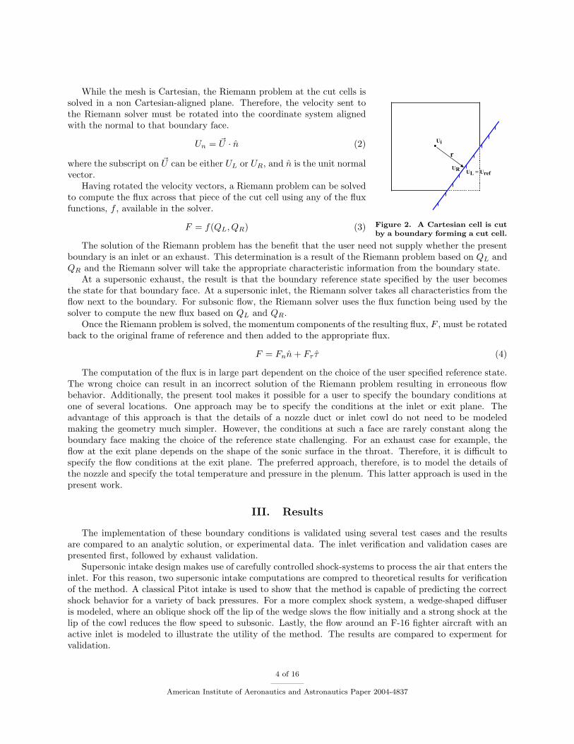
In order to solve the Riemann problem at a boundary of a cut-cell marked for inlet/exhaust, the user mustspecify a reference state that corresponds to the flow condition inside this boundary. Such a cell is depictedin Fig. 2 where the user-specified flow conditions inside the boundary are denoted ~QL = ~Qref . The flowconditions in the cut-cell in the domain adjacent to the boundary are reconstructed from the flow variablesin the local neighborhood and the reconstructed state vector is denoted QR.

QR = Qi + ~r∆Qi (1)

where Qi is the state vector in the Cartesian cell next to the boundary.

3 of 16

American Institute of Aeronautics and Astronautics Paper 2004-4837

Ui

r

UL = UrefUR

Figure 2. A Cartesian cell is cutby a boundary forming a cut cell.

While the mesh is Cartesian, the Riemann problem at the cut cells issolved in a non Cartesian-aligned plane. Therefore, the velocity sent tothe Riemann solver must be rotated into the coordinate system alignedwith the normal to that boundary face.

Un = ~U · n̂ (2)

where the subscript on ~U can be either UL or UR, and n̂ is the unit normalvector.

Having rotated the velocity vectors, a Riemann problem can be solvedto compute the flux across that piece of the cut cell using any of the fluxfunctions, f , available in the solver.

F = f(QL, QR) (3)

The solution of the Riemann problem has the benefit that the user need not supply whether the presentboundary is an inlet or an exhaust. This determination is a result of the Riemann problem based on QL andQR and the Riemann solver will take the appropriate characteristic information from the boundary state.

At a supersonic exhaust, the result is that the boundary reference state specified by the user becomesthe state for that boundary face. At a supersonic inlet, the Riemann solver takes all characteristics from theflow next to the boundary. For subsonic flow, the Riemann solver uses the flux function being used by thesolver to compute the new flux based on QL and QR.

Once the Riemann problem is solved, the momentum components of the resulting flux, F , must be rotatedback to the original frame of reference and then added to the appropriate flux.

F = Fnn̂ + Fτ τ̂ (4)

The computation of the flux is in large part dependent on the choice of the user specified reference state.The wrong choice can result in an incorrect solution of the Riemann problem resulting in erroneous flowbehavior. Additionally, the present tool makes it possible for a user to specify the boundary conditions atone of several locations. One approach may be to specify the conditions at the inlet or exit plane. Theadvantage of this approach is that the details of a nozzle duct or inlet cowl do not need to be modeledmaking the geometry much simpler. However, the conditions at such a face are rarely constant along theboundary face making the choice of the reference state challenging. For an exhaust case for example, theflow at the exit plane depends on the shape of the sonic surface in the throat. Therefore, it is difficult tospecify the flow conditions at the exit plane. The preferred approach, therefore, is to model the details ofthe nozzle and specify the total temperature and pressure in the plenum. This latter approach is used in thepresent work.

III. Results

The implementation of these boundary conditions is validated using several test cases and the resultsare compared to an analytic solution, or experimental data. The inlet verification and validation cases arepresented first, followed by exhaust validation.

Supersonic intake design makes use of carefully controlled shock-systems to process the air that enters theinlet. For this reason, two supersonic intake computations are compred to theoretical results for verificationof the method. A classical Pitot intake is used to show that the method is capable of predicting the correctshock behavior for a variety of back pressures. For a more complex shock system, a wedge-shaped diffuseris modeled, where an oblique shock off the lip of the wedge slows the flow initially and a strong shock at thelip of the cowl reduces the flow speed to subsonic. Lastly, the flow around an F-16 fighter aircraft with anactive inlet is modeled to illustrate the utility of the method. The results are compared to experment forvalidation.

4 of 16

American Institute of Aeronautics and Astronautics Paper 2004-4837

Following the inlet results, three exhaust validation test cases are presented followed by a Space Shuttle inthe ascent configuration. The FESTIP geometry with an under-expanded plume is computed and comparedto an experiment. A tangent-ogive missile body at M = 0.9 for which the plume effects the pressure on therear part of the missile body is simulated for several plume shapes. The plume shape is controlled by thepressure in the plenum chamber. The results are compared to experimental pressure data. A hypersonic freejet is also computed and the results are compared to experiment validating the usefulness of the capabilityfor very large plenum to free stream pressure ratios. Finally, the full Space Shuttle launch vehicle with allthe details of attachment hardware, etc. is modeled with plumes to demonstrate a practical application ofthe method.

A. Pitot intake

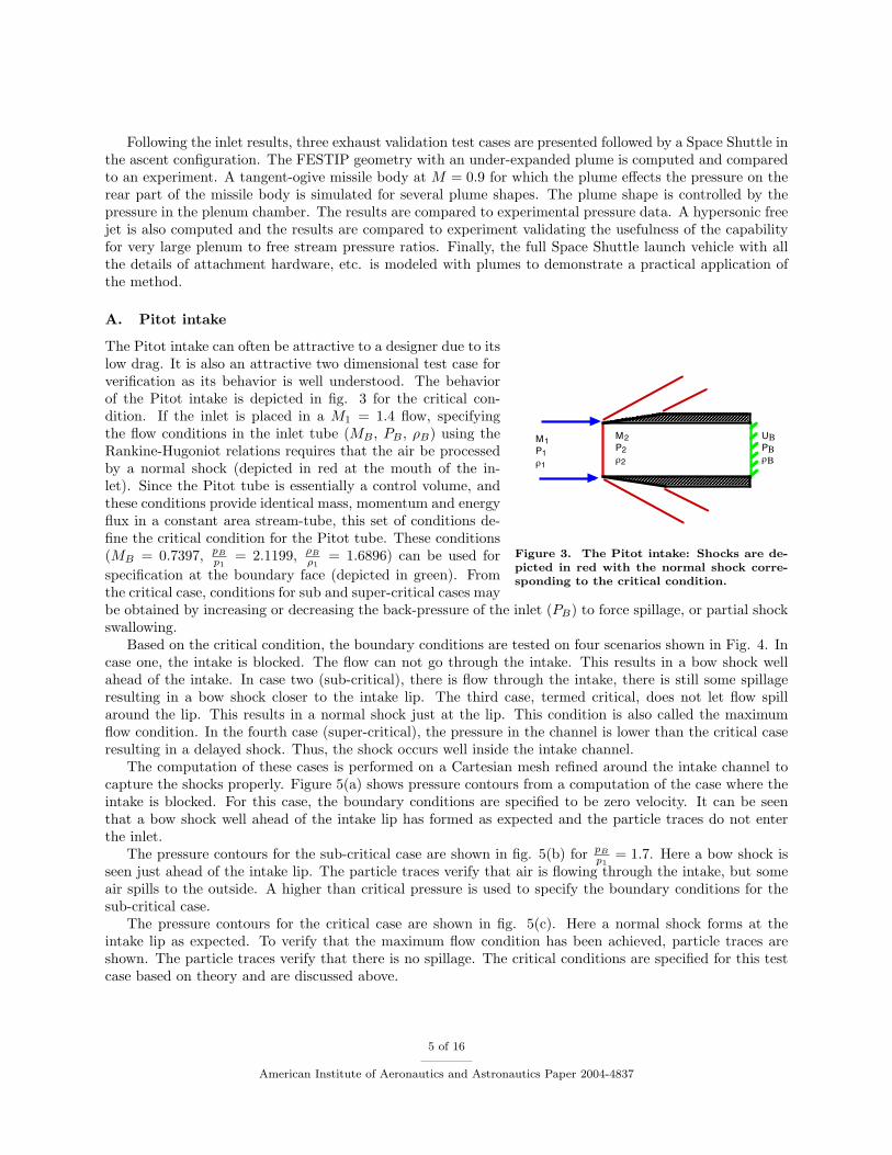
M1P1ρ1

UBPBρΒ

M2P2ρ2

Figure 3. The Pitot intake: Shocks are de-picted in red with the normal shock corre-sponding to the critical condition.

The Pitot intake can often be attractive to a designer due to itslow drag. It is also an attractive two dimensional test case forverification as its behavior is well understood. The behaviorof the Pitot intake is depicted in fig. 3 for the critical con-dition. If the inlet is placed in a M1 = 1.4 flow, specifyingthe flow conditions in the inlet tube (MB , PB , ρB) using theRankine-Hugoniot relations requires that the air be processedby a normal shock (depicted in red at the mouth of the in-let). Since the Pitot tube is essentially a control volume, andthese conditions provide identical mass, momentum and energyflux in a constant area stream-tube, this set of conditions de-fine the critical condition for the Pitot tube. These conditions(MB = 0.7397, pB

p1= 2.1199, ρB

ρ1= 1.6896) can be used for

specification at the boundary face (depicted in green). Fromthe critical case, conditions for sub and super-critical cases maybe obtained by increasing or decreasing the back-pressure of the inlet (PB) to force spillage, or partial shockswallowing.

Based on the critical condition, the boundary conditions are tested on four scenarios shown in Fig. 4. Incase one, the intake is blocked. The flow can not go through the intake. This results in a bow shock wellahead of the intake. In case two (sub-critical), there is flow through the intake, there is still some spillageresulting in a bow shock closer to the intake lip. The third case, termed critical, does not let flow spillaround the lip. This results in a normal shock just at the lip. This condition is also called the maximumflow condition. In the fourth case (super-critical), the pressure in the channel is lower than the critical caseresulting in a delayed shock. Thus, the shock occurs well inside the intake channel.

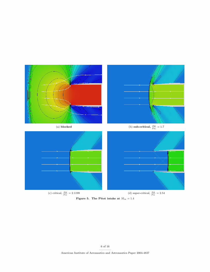
The computation of these cases is performed on a Cartesian mesh refined around the intake channel tocapture the shocks properly. Figure 5(a) shows pressure contours from a computation of the case where theintake is blocked. For this case, the boundary conditions are specified to be zero velocity. It can be seenthat a bow shock well ahead of the intake lip has formed as expected and the particle traces do not enterthe inlet.

The pressure contours for the sub-critical case are shown in fig. 5(b) for pB

p1= 1.7. Here a bow shock is

seen just ahead of the intake lip. The particle traces verify that air is flowing through the intake, but someair spills to the outside. A higher than critical pressure is used to specify the boundary conditions for thesub-critical case.

The pressure contours for the critical case are shown in fig. 5(c). Here a normal shock forms at theintake lip as expected. To verify that the maximum flow condition has been achieved, particle traces areshown. The particle traces verify that there is no spillage. The critical conditions are specified for this testcase based on theory and are discussed above.

5 of 16

American Institute of Aeronautics and Astronautics Paper 2004-4837

(a) blocked (b) sub-critical, pBp∞

= 1.7

(c) critical, pBp∞

= 2.1199 (d) super-critical, pBp∞

= 2.54

Figure 5. The Pitot intake at M∞ = 1.4

6 of 16

American Institute of Aeronautics and Astronautics Paper 2004-4837

M∞>1

M<1 M∞

Blocked Sub-critical

Critical Super-critical

Figure 4. The Pitot intake: Depicted are the four states at whichthe boundary conditions are tested.

The pressure contours for the super-critical case are shown in fig. 5(d) forpB

p1= 2.54. Here the normal shock is seen

inside the intake channel. The particletraces verify that no air spills to the out-side of the lip. A lower than critical pres-sure is used to create the super-criticalconditions.

B. Two-shock wedge diffuser

A 2-shock wedge-shaped inlet, depictedin fig. 6, is modeled in two dimensions toshow that the method accurately predictsthe effect of the inlet conditions. Thisis an especially demanding test case be-cause it depends on being able to modelprecise shock impingement so that theflow stays parallel to the wedge surface.The inlet is designed to turn the flowthrough the first shock (an oblique shock)such that the flow behind the shock isparallel to the ramp. Mis-predicting theshock strength results in the first (weak) shock missing the upper lip and thus never setting up the secondshock. If the correct shock strength is obtained, a strong shock at the cowl lip forms, turning the flow parallelto the axis of the inlet and slowing the flow to subsonic speeds. The strong shock impinges precisely at thelower wall corner so that the flow is turned only by the shock. Missing any of these details results in anerroneous solution which takes the form of either a system of reflecting oblique shocks in the duct or a singledetached weak shock. As with the critical Pitot inlet case, flow at the inlet face where the boundary stateis specified is subsonic.

Wea

k Sh

ock

Strong Shock

M=2P1ρ1

M2P2ρ2

M3P3ρ3Zs Ztube

Figure 6. The two shock Wedge diffuser

The exact solution to the flow in thisinlet can be derived using the obliqueshock tables for the first shock[9]. Fora free stream speed of M∞ = 2.0, thepressure and density jumps across theweak shock are 1.3154 and 1.2156 respec-tively with the speed behind the shockcorresponding to M = 1.82125. TheMach number behind the strong shock(0.61965) for a turn angle of 5◦ is readfrom the strong shock branch of theoblique shock charts and corresponds to a shock angle of 86.36◦. The corresponding pressure and den-sity jumps are 3.6875 and 2.3871 respectively.

A geometry of the 5◦ wedge and inlet duct that corresponds to the maximum flow condition is created.The area of the inlet is computed using the conservation relation,

ρ1u1Zs = ρ3u3Ztube (5)

where Zs is the capture area, ρ1 and u1 correspond to the free stream conditions, and ρ3 and u3 correspond tothe density, and speed in the tube of size Ztube. For the present test case, Zs = 0.2069 and Ztube = 0.17799for a 5◦ wedge and a wedge length of 0.4.

7 of 16

American Institute of Aeronautics and Astronautics Paper 2004-4837

Figure 7. Pressure contours for the two shock Wedge diffuser

The resulting flow field is shown in figure 7. With a back pressure of 4.8505 and back density of 2.9017,the computed solution is in excellent agreement with the exact solution.

C. F-16

Figure 8. Velocity Magnitude for an F-16 with active inlet and exhaust at M∞ = 0.85 and α = 16◦

The present method can be easily applied to a vehicle with complex geometry. An F-16 is simulatedwith an active inlet as well as an active exhaust for demonstration. Specialized methods with the intentof capturing the effects of an active inlet on the pressure close to the inlet duct have been used for F-16simulation in the past[1, 10]. Based on these, a set of reference conditions that do not modify the conditionsat the inlet are specified. A plume is simulated with a high velocity exhaust.

8 of 16

American Institute of Aeronautics and Astronautics Paper 2004-4837

Figure 9. Contours of the coefficient of pressure for an F-16 with active inlet and exhaust at M∞ = 0.85 andα = 16◦; circumferential cut location indicated in magenta

Figure 10. Comparison of computed pressure distributions withexperiment close to the inlet

Figure 8 shows the flow field aroundthe fighter aircraft at M∞ = 0.85 andα = 16.04◦. At the inlet face, the refer-ence Mach number is set to 0.75 and at theexhaust, the reference Mach number is setto 2.2 leaving the pressure at both equal tothe upstream ambient pressure. In this fig-ure, the colors represent the speed of theflow. Stream traces close to the inlet ductshow flow entering the inlet as well as goingaround the inlet. The effect of the flow intoan active inlet can be seen in the changein pressure in the vicinity of the inlet cowl.Figure 9 shows contours of the pressure co-efficient on the surface of the vehicle. Ablack line in the figure represents the cir-cumferential cut along which values of thepressure coefficient are compared in Fig. 10with and without inlet modeling. S in theplot is the arc length along the cross sectionof the fuselage starting at the bottom. The difference in these pressure distributions affirms the need formodeling an active inlet. The pressure coefficient in Fig. 10 is also compared to experiment[10] and agreesclosely. The slight discrepancy in the pressure near S = 0.4 may be due to the addition of the gun-portgeometry for the M61 A1 Vulcan 20mm gatling gun system in the present simulation.

D. FESTIP

In addition to being able to predict the inlet flows correctly, the method also allows accurate prediction ofthe effects of an exhaust plume. We first focus our attention on the qualitative features of the flow field withthe plume. In order to verify that we obtain a properly sized plume and that we are able to capture theeffects of the plume on the flow field, the FESTIP vehicle is simulated at Mach 2.98 with plume conditionsspecified [7]. The resulting flow field is shown in fig. 11(b) and is compared to a Schlieren photograph (fig.11(a)) from the experiment. The comparison shows that the present method correctly predicts not only thebow shock structure due to the vehicle and sting, but also correctly captures the extent of the plume, and

9 of 16

American Institute of Aeronautics and Astronautics Paper 2004-4837

(a) Experimental (b) Computational

Figure 11. Density contours on the surface of the FESTIP and the center plane at M∞ = 2.98 compared toexperiment[7]

compression shock which forms near the exhaust.

E. Tangent-ogive plume

A plume often has an effect on the flow near the aft-body area, where flow turning to accommodate theplume can put a shock on the aft part of the vehicle, drastically modifying the surface pressure and velocitiesand thus effecting forces and moments. This effect is especially noticeable for under-expanded plumes. Thus,a quantitative validation of the plume capability of the boundary conditions can be performed by examiningthe pressure variation on the body with the size of the plume. An ogive-shaped missile for which the effectof the plume on the surface of the aft-body is experimentally documented for several plume conditions ischosen.

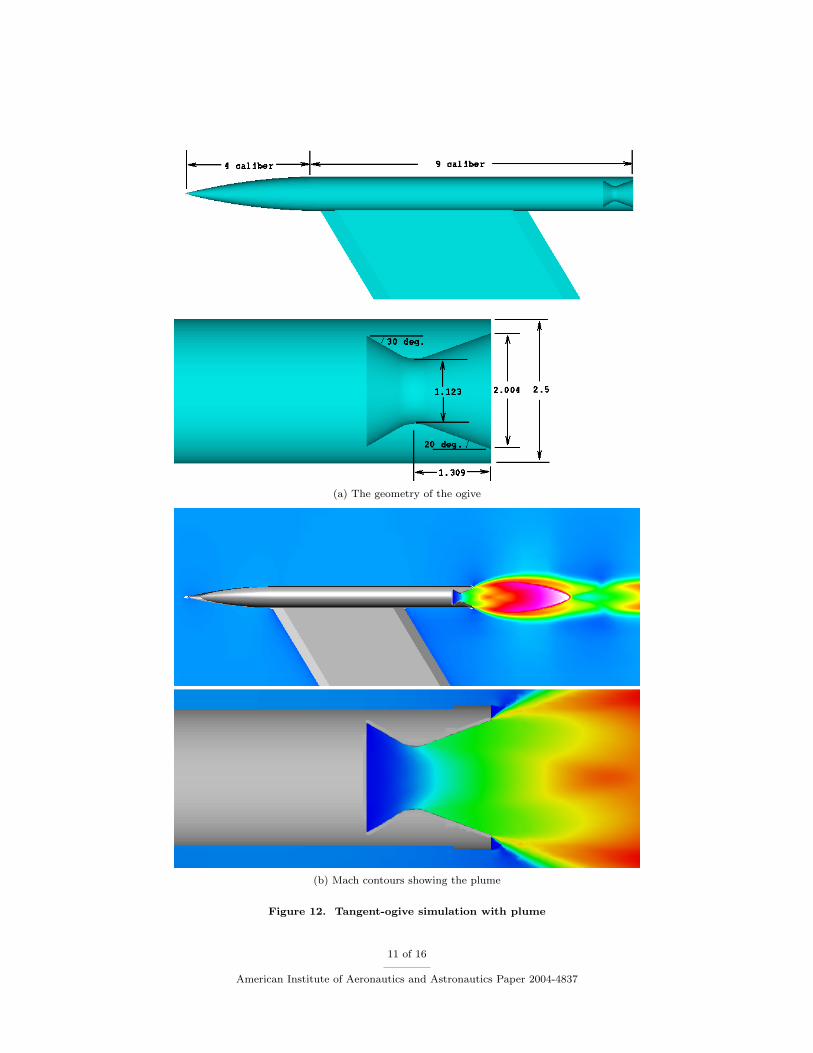
A strut-mounted body of revolution (see Fig. 12(a)) with a cylindrical after-body is used in an experimentby Burt [8] at M = 0.9 and M = 1.2 with zero angle of attack. This case has been more recently computedby Raghunathan et. al [11] using a viscous technique. The model has a 4-caliber tangent-ogive nose attachedto a 9-caliber cylindrical body. A 20 deg . conical nozzle with a design Mach number of 2.7 is modeled tomatch the experiment.

Conditions are specified at the vertical face in the plenum chamber which correspond to the experimentalconditions, including the pressure ratio between the plenum and the free stream. The specification of thepressure in the plenum provides the mechanism by which the air is pushed through the throat and the nozzle.The resulting plume is depicted by Mach number contours in Fig. 12(b) where blue denotes low speed flowsuch as that in the plenum, white denotes the high speed flow at approximately Mach 7 and the colors inbetween denote intermediate values.

The pressure on the surface of the cylindrical after-body is reported by the experiment [8] for a rangeof pressure ratios. The lowest pressure ratios correspond to an over-expanded plume while high pressureratios correspond to an under-expanded plume. A blockage to the main flow develops as a result of theunder-expanded plume. The plume grows larger with higher pressure ratios. Thus, at high pressure ratiosthe plume has a larger effect on the aerodynamics in the region of the cylindrical after-body. This effect canbe seen by examining the changes in pressure on the after-body. The pressure on the after-body is thereforecompared to the experiment in Fig. 13(a) and shows good agreement in both trend and value.

A similar plot on the same body for free stream Mach number of 1.2 is also shown in figure 13(b). Forthis supersonic case, the vehicle develops a shock on the cylindrical after-body due to the blockage from theunder-expanded plume. Due to the boundary layer development, the compression in the experiment is not

10 of 16

American Institute of Aeronautics and Astronautics Paper 2004-4837

(a) The geometry of the ogive

(b) Mach contours showing the plume

Figure 12. Tangent-ogive simulation with plume

11 of 16

American Institute of Aeronautics and Astronautics Paper 2004-4837

(a) M∞ = 0.9 (b) M∞ = 1.2

Figure 13. Pressure on the surface of the ogive compared to Experiments[8] (x=0 is the base of the ogivebody)

as abrupt as the inviscid simulation and as a result, the shock location is not well-predicted by the solutionof the Euler equations, but the effect on the moment is similar.

F. Under-expanded jet

Table 1. Flow conditions upstream of the orifice for the under-expanded jet

case PT TT Pback

1 1.3 atm 297 K 2.68 × 10−4 atm2 1.13 atm 297 K 1.37 × 10−4 atm

A hypersonic, under-expanded, free jet, such as one emanating from a reaction control system (RCS),is a challenging problem due to extremely large pressure ratios producing a large under-expanded plumeand the presence of a strong shock. The jet is released from a small orifice into near-vacuum conditionssuch that the ratio of the plenum pressure (PT ) to the ambient flow is approximately 3500. This severechange in conditions results in a jet that accelerates to Mach 16 and has gradients in radial as well as axialdirections [12]. The jet is terminated by a strong shock which brings the flow from M = 16 to subsonicspeeds. The experiment was performed at two sets of conditions which are given in table 1.

A plot of the velocity magnitude is shown for case 1 in fig. 14(a) and compared to planar laser inducediodine fluorescence (PLIIF) measurements from experiment [12]. The bell-shaped plume is visible with thestrong shock at the edge of the plume. Both the shape of the plume and the location of the shock agreeextremely well with experiment and are similar to the computational results presented by McDaniel et. al[12]. The speed of the flow along the centerline is compared next. The comparison is shown in Fig. 14(b)along with theoretical predictions from Ashkenas & Sherman [13]. The acceleration of the flow is properlycaptured, but the location of the shock is slightly ahead of the experiment.

Further comparisons are made for case 2 by plotting the pressure and temperature along the centerlinein Figs. 15(a) and 15(b) respectively. In this case, the higher pressure in the plenum moved the shockfurther downstream as compared to case 1 and a larger plume is obtained. The pressure and temperaturealong the centerline agree well with the theory of Ashkenas & Sherman. The results also agree closely to theexperiment and compare well to the viscous simulations by McDaniel et. al [12].

12 of 16

American Institute of Aeronautics and Astronautics Paper 2004-4837

(a) Global velocity contours (b) Speed along the centerline

Figure 14. Velocity comparisons for an under-expanded free jet (case 1)

(a) Pressure along the centerline (b) Temperature along the centerline

Figure 15. Pressure and temperature comparisons for an under-expanded free jet (case 2)

13 of 16

American Institute of Aeronautics and Astronautics Paper 2004-4837

G. Space Shuttle

Figure 16. Mach number contours on the Space Shuttle in ascent at M∞ = 2.5

During the STS-107 accident investigation, coupled 6-DOF simulations of debris emanating from theSpace Shuttle Launch Vehicle (SSLV) during ascent were performed using Cartesian methods[14]. In thesesimulations the plumes emanating from the shuttle main engines (SSME) and solid rocket boosters (SRB)were ignored. While the plumes had little effect on the flowfield ahead of the wing leading edge, andhence were not critical for the debris simulations during the accident investigation, the current methodof simulating the engine plumes does provide higher-fidelity with little additional complexity. The plumeexhausts on the shuttle are underexpanded, and hence have a large effect on the flowfield and aerodynamicloads near the aft end of the vehicle. This is especially true for the bluff aft bodies of the shuttle orbiter andexternal tank. By ignoring the plumes the flow separates around these bluff bodies leading to large-scaleunsteadiness. The plumes entrain much of this separated flow, leading to less flow unsteadiness and loadexcursions. Figure 16 shows an example calculation of the SSLV flowfield at Mach 2.5 and 0.0◦ angle ofattack, with the SSME and SRB plumes operating at flight conditions. As with the previous examples, theexhaust nozzle geometry is modeled up to the plenum chamber. The plenum conditons were obtained froma real-gas simulation[15]. The Mach number contours on the body and centerline of the SSLV are shown,along with the plumes (blue is low, red is high). The shock waves are well resolved, and the low speed flowon the aft end of the orbiter and external tank is apparent. The high Mach number core of each plume isvisible within the the SSME and SRB bell nozzles. The SSME and SRB nozzles are capable of gimbalingin this component geometry, and a companion paper[16] contains an automated parametric study of the

14 of 16

American Institute of Aeronautics and Astronautics Paper 2004-4837

SSLV flowfield including the effect of engine gimbal angle. This provides an automated, efficient methodof simulating the complete SSLV geometry in any flight configuration. This ability can be used to providehigh-fidelity, rapid-response,launch-day simulations, or other time-critical analysis.

IV. Concluding remarks

A boundary condition based on flux update through the solution of a Riemann problem is presentedwithin a Cartesian method. The procedure is shown to be an accurate engineering tool to model inlet flowsand exhaust plumes on aircraft, spacecraft and missiles. The additional boundary model has no effect onrobustness, or convergence of the multigrid algorithm and the CFL limitations are unchanged.

Several cases are presented for verification and validation. Two supersonic inlet designs that have subsonicflow in the inlet duct are compared to analytic solutions to validate the method for inlet flows. The Pitot inletand the two-shock wedge-shaped inlet show that the method accurately predicts the strength and locationof a system of oblique and normal shocks based on user-specified conditions inside the inlet duct. Thecomputational results compare extremely well with the gas dynamics theory and thus validate the capabilityfor accurately modeling complex inlet flow and shock patterns given the conditions inside an inlet duct.

Two exhaust plume cases are compared to experiment to validate the exhaust capability of the method.The FESTIP test case shows that the size and shape of the plume as well as its effects on the flow field arewell predicted. A simple ogive-shaped missile is simulated with exhaust and the pressures on the after-bodyare compared to an experiment for various chamber pressures which result in different plume sizes. It isconcluded that the modeling of the nozzle internal geometry is preferable in order to accurately predict thesonic disk and ultimately the plume shape.

The inlet/exit boundary conditions are also applied to cases of practical interest with complex geometry.The inlet modeling of an F-16 fighter aircraft shows dramatic effect on the local flow in the vicinty of theinlet cowl. The exhaust from the rocket engines of a Space Shuttle Launch Vehicle (SSLV) is presenteddemonstrating the usefulness of the simple engineering method presented for a non-expert user to specifyinlets and exhausts to obtain proper modeling of their effects.

The usefulness of this boundary conditions infrastructure can be enhanced by allowing the user to mimica pressure jump at specified locations in the flow field instead of simply specifying a state. Such an “actuator-disk” type boundary condition would simplify modeling of fans, ducted fans, and helicopter rotors. Further-more, the viscous layer close to the wall can have a substantial effect on the forces and moments. To obtainthe gross effects of viscosity, this method can be extended with a boundary layer model to accurately captureviscous/inviscid interaction. Finally, the present model is validated for cold gas with no chemical reactions.Species modeling is necessary to extend the method to treat hot gas and chemically reacting flows.

V. Acknowledgment

The authors wish to thank Mike Olsen and Dr. William Chan of NASA Ames for their invaluable inputduring the course of this work. The authors would also like to thank Dr. M. Berger of NYU for usefuldiscussions and Nick Georgiadis of NASA Glenn Research Center for help in obtaining experimental dataand configurations. Dr. Murman was supported by NASA Ames Research Center (contract NAS2-00062)during this work.

References

1 Flores, J., Chaderjian, N., and Sorenson, R., “Simulation of Transonic Viscous Flow over a Fighter-likeConfiguration Including Inlet,” AIAA paper 87-1199.

2 McGhee, R. J., “Jet-Induced Flow Separation on a Lifting Entry Body at Mach Number from 4.00 to

15 of 16

American Institute of Aeronautics and Astronautics Paper 2004-4837

6.00,” NASA Technical Memorandum NASA TM X-1997, NASA Langley Research Center, April 1970.

3 DalBello, T., Georgiadis, N. J., Yoder, D. A., and Keith, T. G., “Computational Study of AxisymmetricOff-design Nozzle Flows,” AIAA paper 2004-0530.

4 Aftosmis, M. J., Berger, M. J., and Melton, J. E., “Robust and efficient Cartesian mesh generation forcomponent-based geometry,” AIAA Paper 97-0196.

5 Aftosmis, M. J., Berger, M. J., and Adomovicius, G., “A parallel multilevel method for adaptively refinedCartesian grids with embedded boundaries,” AIAA Paper 2000-0808.

6 Aftosmis, M. J., Berger, M. J., and Adomovicius, G., “Parallel multigrid on Cartesian meshes withcomplex geometry,” Proc. of the 8th Intl. Conf. on Parallel CFD , Trondhiem Norway, June 2000.

7 Bannink, W. J., Houtman, E. M., and Bakker, P. G., “Base Flow / Underexpanded Exhaust PlumeInteraction in a Supersonic External Flow,” AIAA paper 98-1598.

8 Burt, J. R., “An Investigation of the Effectiveness of Several Devices in Simulating a Rocket Plume atFree Stream Mach Numbers of 0.9 to 1.2,” Tech. Rep. RD-TR-71-22, U. S. Army Missile Command,Redstone Arsenal, Alabama, September 1971.

9 Staff, A. R., “Equations, Tables, and Charts for Compressible Flow,” Tech. rep., Ames AeronauticalLaboratory, Moffett Field, CA, 1953.

10 Huband, G. W., Shang, J. S., and Aftosmis, M. J., “Numerical Simulation of an F-16A at Angle ofAttack,” J. of Aircraft , Vol. 27, No. 10, October 1990, pp. 886–892.

11 Raghunathan, S., Kim, H. D., Benard, E., Malon, P., and Harrison, R., “Plume Interference Effects onMissile Bodies,” J. Spacecraft , Vol. 40, No. 1, 2002, pp. 136–138.

12 McDaniel, J. C. J., Glass, C. E., Staack, D., and Miller, C. G. I., “Experimental and ComputationalComparison of an Underexpanded Jet Flowfield,” AIAA Paper 2002-0305.

13 Ashkenas, H. and Sherman, F., “The Structure and Utilization of Supersonic Free Jets in Low DensityWind Tunnels,” Rarefied Gas Dynamics, edited by J. H. de Leeuw, Vol. II, Supplement 3 of Advancesin Applied Mechanics, Academic Press, 1966, pp. 84–105, Section 7: Experimental Methods in RarefiedGas Dynamics.

14 Gomez, R., Vicker, D., Rogers, S., Aftosmis, M., Chan, W., and Meakin, R., “STS-107 InvestigationAscent CFD Support,” AIAA paper 2004-2226.

15 D’Agostino, M., Marshall Space Flight Center, NASA, Huntsville, AL, Private communication.

16 Murman, S., Aftosmis, A., and Nemec, M., “Parameter Studies Using a Cartesian Method,” AIAA paper2004-5076.

16 of 16

American Institute of Aeronautics and Astronautics Paper 2004-4837