99
Valuation: Lecture Note Packet 1 Intrinsic Valuation Dr. Yaqoub Alabdullah 1

Valuation: Lecture Note Packet 1
Intrinsic Valuation
Dr. Yaqoub Alabdullah
1

2
The essence of intrinsic value
In intrinsic valuation, you value an asset based upon its fundamentals (or intrinsic characteristics).
For cash flow generating assets, the intrinsic value will be a function of the magnitude of the expected cash flows on the asset over its lifetime and the uncertainty about receiving those cash flows.
Discounted cash flow valuation is a tool for estimating intrinsic value, where the expected value of an asset is written as the present value of the expected cash flows on the asset, with either the cash flows or the discount rate adjusted to reflect the risk.
2

3
The two faces of discounted cash flow valuation
The value of a risky asset can be estimated by discounting the expected cash flows on the asset over its life at a risk-adjusted discount rate:
where the asset has an n-year life, E(CFt) is the expected cash flow in period t and r is a discount rate that reflects the risk of the cash flows.
Alternatively, we can replace the expected cash flows with the guaranteed cash flows we would have accepted as an alternative (certainty equivalents) and discount these at the riskfree rate:
where CE(CFt) is the certainty equivalent of E(CFt) and rf is the riskfree rate.
3
4
Risk Adjusted Value: Two Basic Propositions
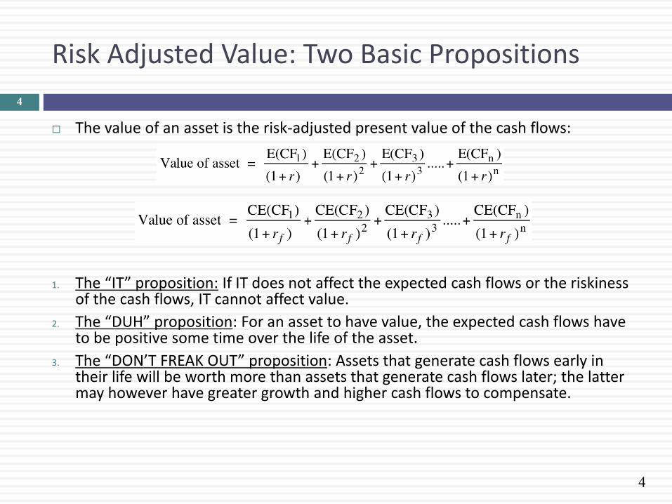
The value of an asset is the risk-adjusted present value of the cash flows:
1. The “IT” proposition: If IT does not affect the expected cash flows or the riskiness of the cash flows, IT cannot affect value.
2. The “DUH” proposition: For an asset to have value, the expected cash flows have to be positive some time over the life of the asset.
3. The “DON’T FREAK OUT” proposition: Assets that generate cash flows early in their life will be worth more than assets that generate cash flows later; the latter may however have greater growth and higher cash flows to compensate.
4
5
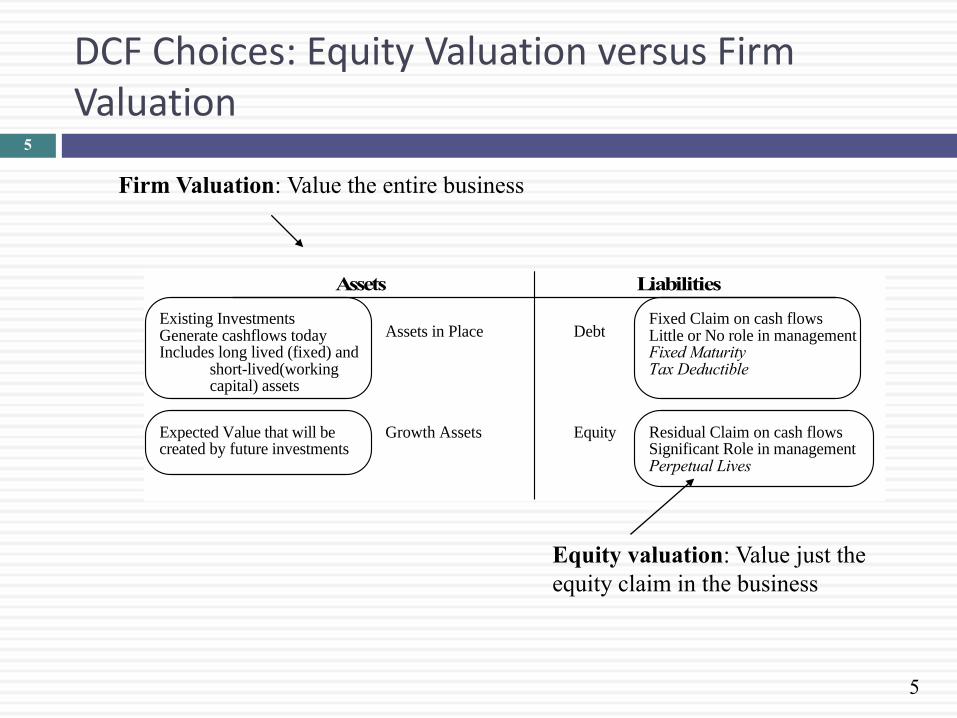
DCF Choices: Equity Valuation versus Firm Valuation
Assets Liabilities
Assets in Place Debt
Equity
Fixed Claim on cash flowsLittle or No role in managementFixed MaturityTax Deductible
Residual Claim on cash flowsSignificant Role in managementPerpetual Lives
Growth Assets
Existing InvestmentsGenerate cashflows todayIncludes long lived (fixed) and
short-lived(working capital) assets
Expected Value that will be created by future investments
Equity valuation: Value just the
equity claim in the business
Firm Valuation: Value the entire business
5

6
Equity Valuation
Assets Liabilities
Assets in Place Debt
Equity
Discount rate reflects only the cost of raising equity financing
Growth Assets
Figure 5.5: Equity Valuation
Cash flows considered are cashflows from assets, after debt payments and after making reinvestments needed for future growth
Present value is value of just the equity claims on the firm
6
7
Firm Valuation
Assets Liabilities
Assets in Place Debt
Equity
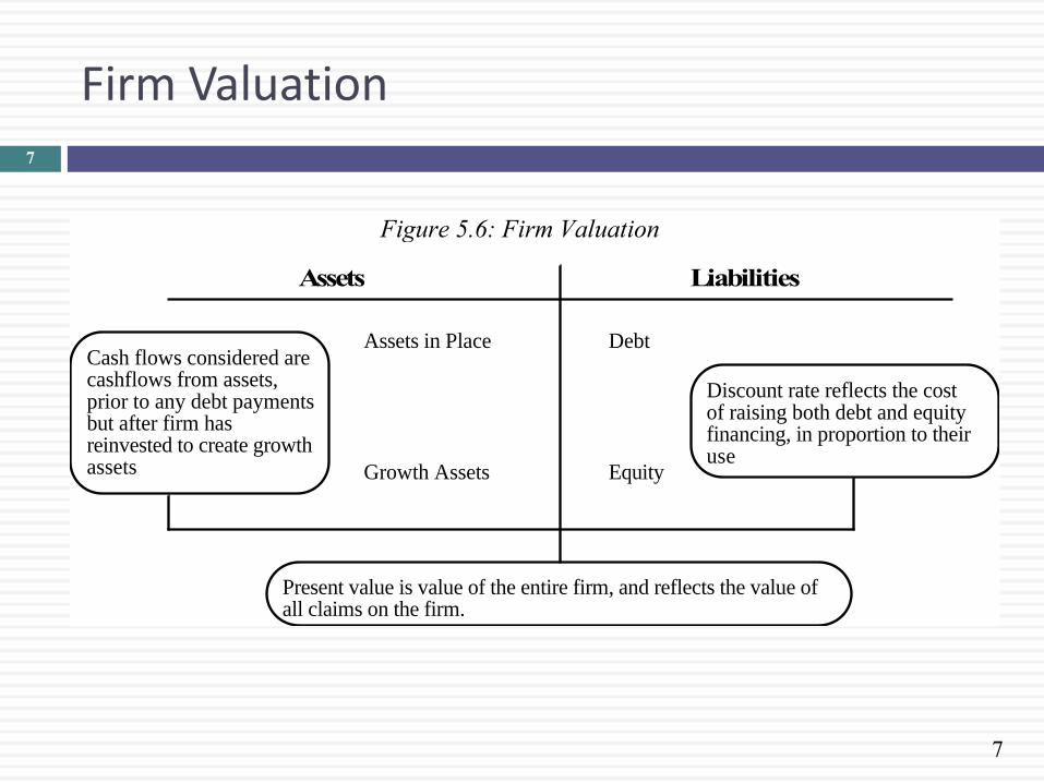
Discount rate reflects the cost of raising both debt and equity financing, in proportion to their use
Growth Assets
Figure 5.6: Firm Valuation
Cash flows considered are cashflows from assets, prior to any debt paymentsbut after firm has reinvested to create growth assets
Present value is value of the entire firm, and reflects the value of all claims on the firm.
7

8
Firm Value and Equity Value
To get from firm value to equity value, which of the following would you need to do?
a. Subtract out the value of long term debt
b. Subtract out the value of all debt
c. Subtract the value of any debt that was included in the cost of capital calculation
d. Subtract out the value of all liabilities in the firm
Doing so, will give you a value for the equity which is
a. greater than the value you would have got in an equity valuation
b. lesser than the value you would have got in an equity valuation
c. equal to the value you would have got in an equity valuation
8
9
Cash Flows and Discount Rates
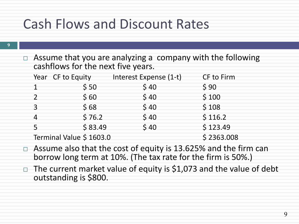
Assume that you are analyzing a company with the following cashflows for the next five years. Year CF to Equity Interest Expense (1-t) CF to Firm
1 $ 50 $ 40 $ 90
2 $ 60 $ 40 $ 100
3 $ 68 $ 40 $ 108
4 $ 76.2 $ 40 $ 116.2
5 $ 83.49 $ 40 $ 123.49
Terminal Value $ 1603.0 $ 2363.008
Assume also that the cost of equity is 13.625% and the firm can borrow long term at 10%. (The tax rate for the firm is 50%.)
The current market value of equity is $1,073 and the value of debt outstanding is $800.
9

10
Equity versus Firm Valuation
Method 1: Discount CF to Equity at Cost of Equity to get value of equity Cost of Equity = 13.625%
Value of Equity = 50/1.13625 + 60/1.136252 + 68/1.136253 + 76.2/1.136254 + (83.49+1603)/1.136255 = $1073
Method 2: Discount CF to Firm at Cost of Capital to get value of firm Cost of Debt = Pre-tax rate (1- tax rate) = 10% (1-.5) = 5%
Cost of Capital = 13.625% (1073/1873) + 5% (800/1873) = 9.94%
PV of Firm = 90/1.0994 + 100/1.09942 + 108/1.09943 + 116.2/1.09944 + (123.49+2363)/1.09945 = $1873
Value of Equity = Value of Firm - Market Value of Debt
= $ 1873 - $ 800 = $1073
10
11
First Principle of Valuation
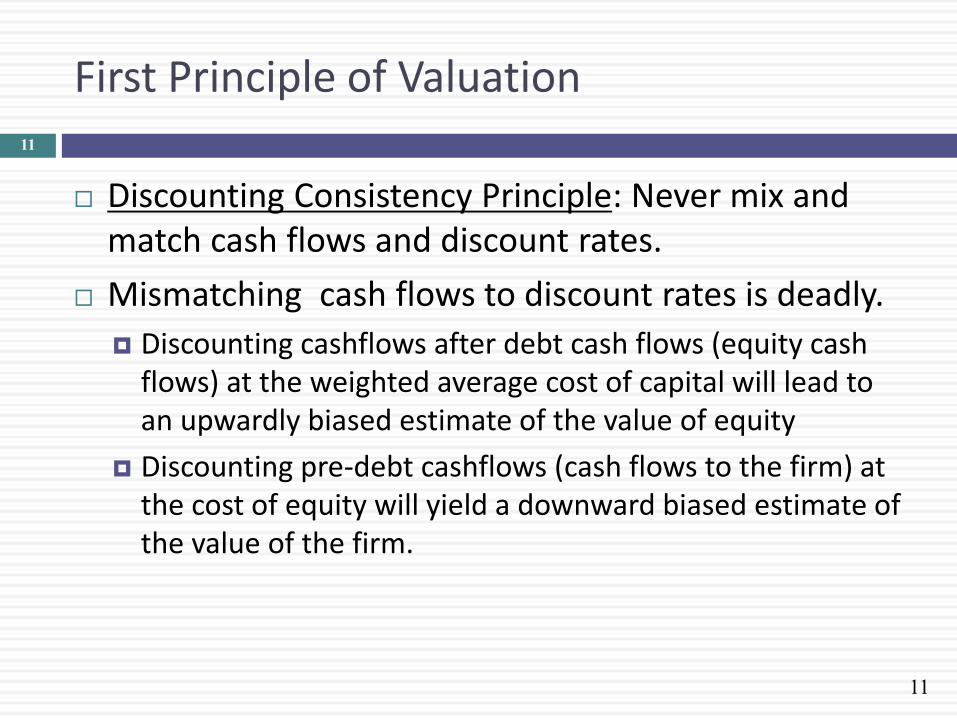
Discounting Consistency Principle: Never mix and match cash flows and discount rates.
Mismatching cash flows to discount rates is deadly.
Discounting cashflows after debt cash flows (equity cash flows) at the weighted average cost of capital will lead to an upwardly biased estimate of the value of equity
Discounting pre-debt cashflows (cash flows to the firm) at the cost of equity will yield a downward biased estimate of the value of the firm.
11
12
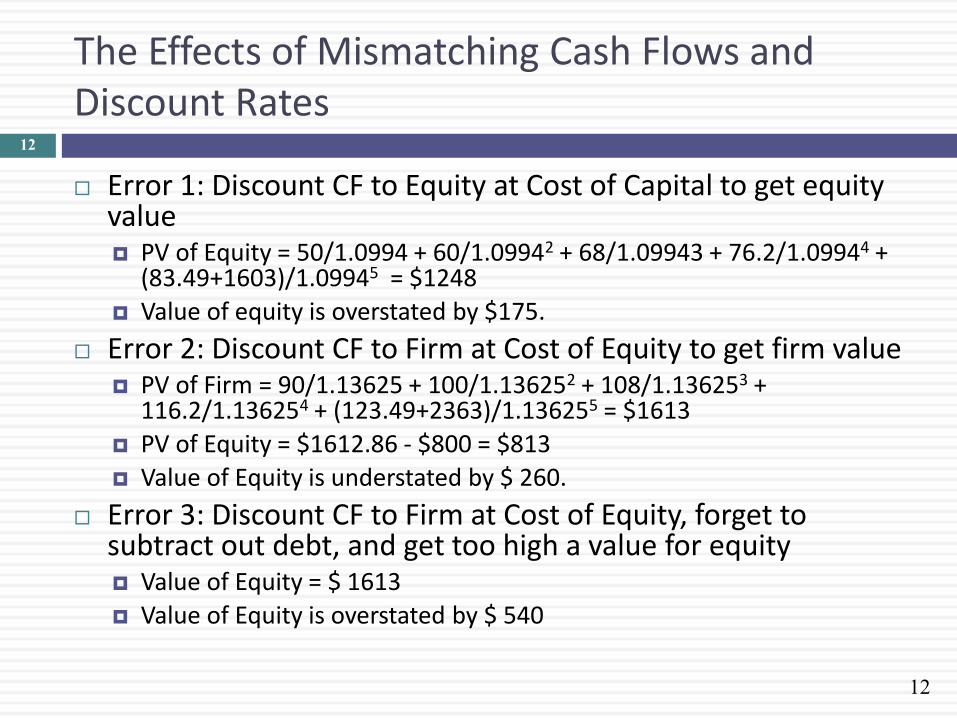
The Effects of Mismatching Cash Flows and Discount Rates
Error 1: Discount CF to Equity at Cost of Capital to get equity value PV of Equity = 50/1.0994 + 60/1.09942 + 68/1.09943 + 76.2/1.09944 +
(83.49+1603)/1.09945 = $1248
Value of equity is overstated by $175.
Error 2: Discount CF to Firm at Cost of Equity to get firm value PV of Firm = 90/1.13625 + 100/1.136252 + 108/1.136253 +
116.2/1.136254 + (123.49+2363)/1.136255 = $1613
PV of Equity = $1612.86 - $800 = $813
Value of Equity is understated by $ 260.
Error 3: Discount CF to Firm at Cost of Equity, forget to subtract out debt, and get too high a value for equity Value of Equity = $ 1613
Value of Equity is overstated by $ 540
12

DISCOUNTED CASH FLOW VALUATION: THE INPUTS
The devil is in the details..
13

14
Discounted Cash Flow Valuation: The Steps
1. Estimate the discount rate or rates to use in the valuation 1. Discount rate can be either a cost of equity (if doing equity valuation) or a cost of
capital (if valuing the firm)
2. Discount rate can be in nominal terms or real terms, depending upon whether the cash flows are nominal or real
3. Discount rate can vary across time.
2. Estimate the current earnings and cash flows on the asset, to either equity investors (CF to Equity) or to all claimholders (CF to Firm)
3. Estimate the future earnings and cash flows on the firm being valued, generally by estimating an expected growth rate in earnings.
4. Estimate when the firm will reach “stable growth” and what characteristics (risk & cash flow) it will have when it does.
5. Choose the right DCF model for this asset and value it.
14
15
Generic DCF Valuation Model 15
16
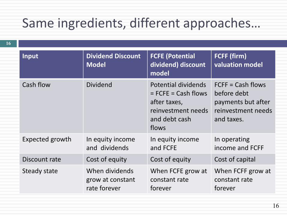
Same ingredients, different approaches…
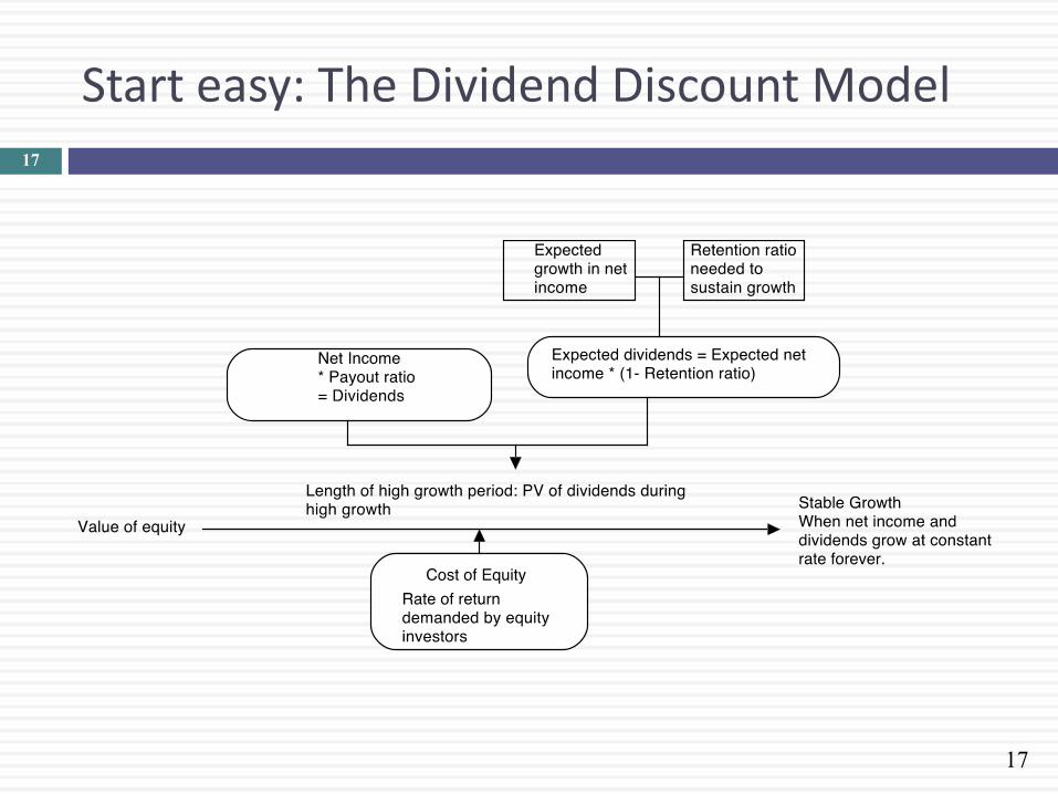
Input Dividend Discount Model
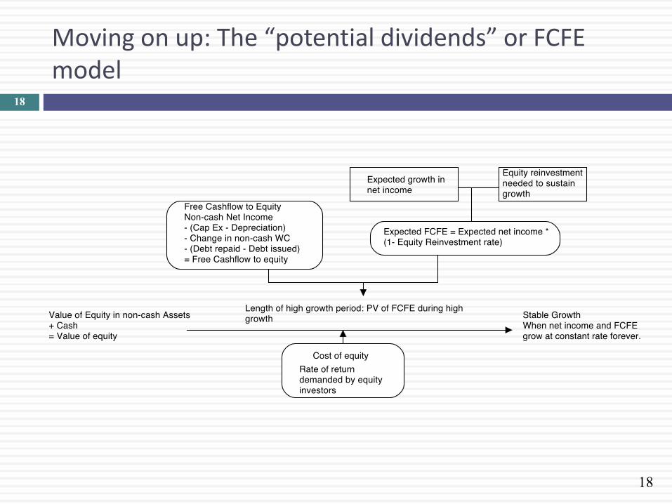
FCFE (Potential dividend) discount model
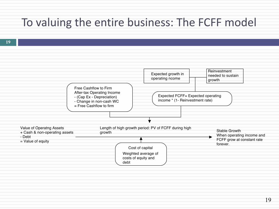
FCFF (firm) valuation model
Cash flow Dividend Potential dividends = FCFE = Cash flows after taxes, reinvestment needs and debt cash flows
FCFF = Cash flows before debt payments but after reinvestment needs and taxes.
Expected growth In equity income and dividends
In equity income and FCFE
In operating income and FCFF
Discount rate Cost of equity Cost of equity Cost of capital
Steady state When dividends grow at constant rate forever
When FCFE grow at constant rate forever
When FCFF grow at constant rate forever
16
17
Start easy: The Dividend Discount Model 17
18
Moving on up: The “potential dividends” or FCFE model
18
19
To valuing the entire business: The FCFF model
19
DISCOUNT RATES
The D in the DCF..
20
21
Estimating Inputs: Discount Rates
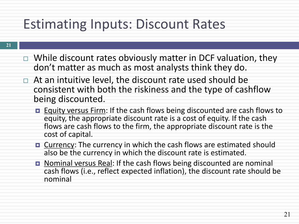
While discount rates obviously matter in DCF valuation, they don’t matter as much as most analysts think they do.
At an intuitive level, the discount rate used should be consistent with both the riskiness and the type of cashflow being discounted. Equity versus Firm: If the cash flows being discounted are cash flows to
equity, the appropriate discount rate is a cost of equity. If the cash flows are cash flows to the firm, the appropriate discount rate is the cost of capital.
Currency: The currency in which the cash flows are estimated should also be the currency in which the discount rate is estimated.
Nominal versus Real: If the cash flows being discounted are nominal cash flows (i.e., reflect expected inflation), the discount rate should be nominal
21

22
Risk in the DCF Model 22
23
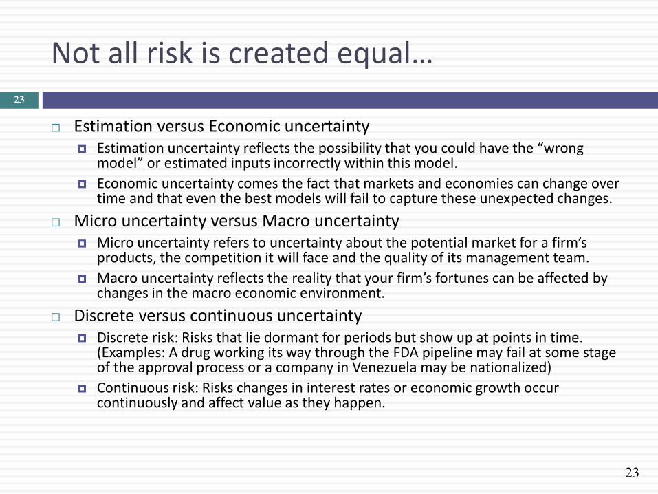
Not all risk is created equal…
Estimation versus Economic uncertainty Estimation uncertainty reflects the possibility that you could have the “wrong
model” or estimated inputs incorrectly within this model.
Economic uncertainty comes the fact that markets and economies can change over time and that even the best models will fail to capture these unexpected changes.
Micro uncertainty versus Macro uncertainty Micro uncertainty refers to uncertainty about the potential market for a firm’s
products, the competition it will face and the quality of its management team.
Macro uncertainty reflects the reality that your firm’s fortunes can be affected by changes in the macro economic environment.
Discrete versus continuous uncertainty Discrete risk: Risks that lie dormant for periods but show up at points in time.
(Examples: A drug working its way through the FDA pipeline may fail at some stage of the approval process or a company in Venezuela may be nationalized)
Continuous risk: Risks changes in interest rates or economic growth occur continuously and affect value as they happen.
23

24
Risk and Cost of Equity: The role of the marginal investor
Not all risk counts: While the notion that the cost of equity should be higher for riskier investments and lower for safer investments is intuitive, what risk should be built into the cost of equity is the question.
Risk through whose eyes? While risk is usually defined in terms of the variance of actual returns around an expected return, risk and return models in finance assume that the risk that should be rewarded (and thus built into the discount rate) in valuation should be the risk perceived by the marginal investor in the investment
The diversification effect: Most risk and return models in finance also assume that the marginal investor is well diversified, and that the only risk that he or she perceives in an investment is risk that cannot be diversified away (i.e, market or non-diversifiable risk). In effect, it is primarily economic, macro, continuous risk that should be incorporated into the cost of equity.
24
25
The Cost of Equity: Competing “ Market Risk” Models
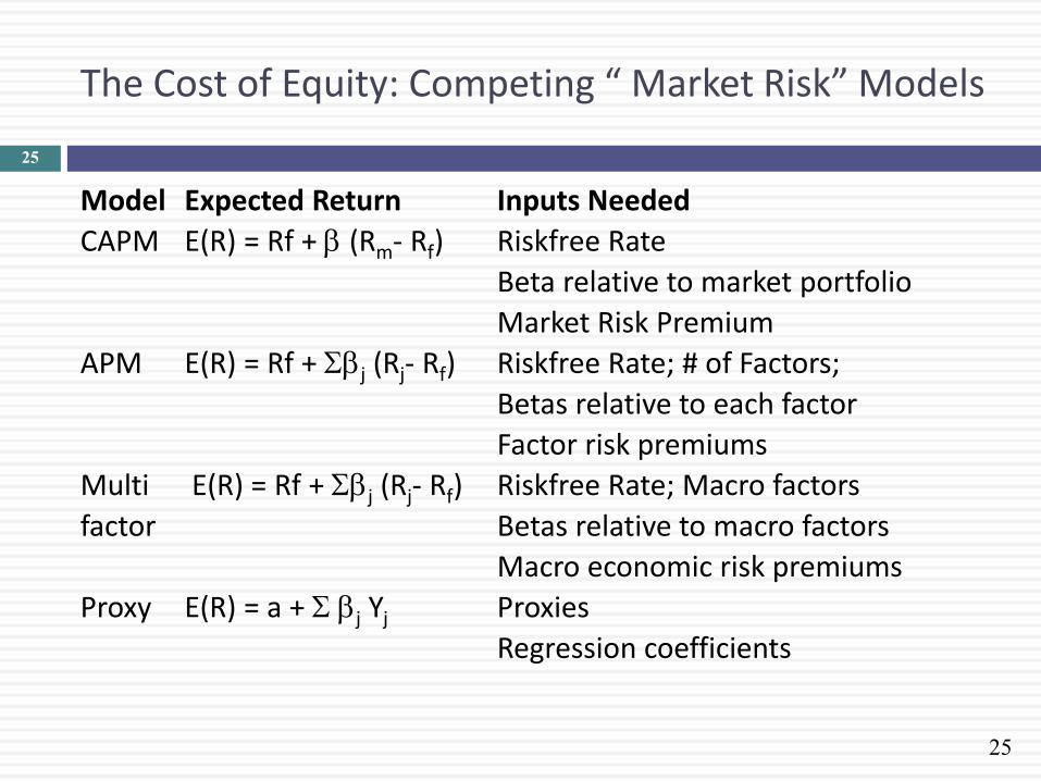
Model Expected Return Inputs Needed
CAPM E(R) = Rf + b (Rm- Rf) Riskfree Rate
Beta relative to market portfolio
Market Risk Premium
APM E(R) = Rf + Sbj (Rj- Rf) Riskfree Rate; # of Factors;
Betas relative to each factor
Factor risk premiums
Multi E(R) = Rf + Sbj (Rj- Rf) Riskfree Rate; Macro factors
factor Betas relative to macro factors
Macro economic risk premiums
Proxy E(R) = a + S bj Yj Proxies
Regression coefficients
25

26
Classic Risk & Return: Cost of Equity
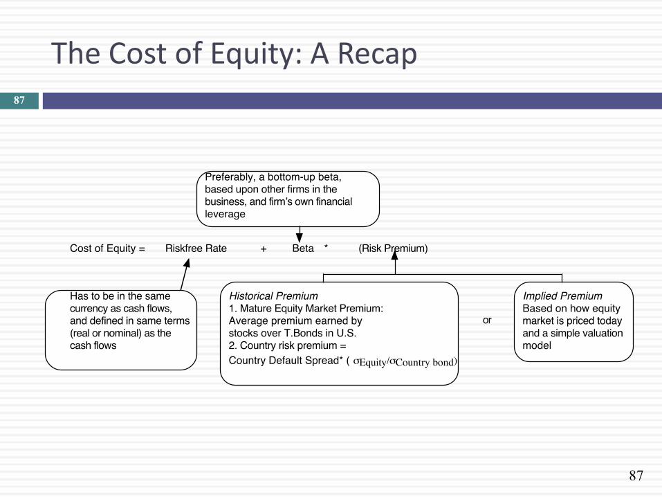
In the CAPM, the cost of equity: Cost of Equity = Riskfree Rate + Equity Beta * (Equity Risk Premium)
In APM or Multi-factor models, you still need a risk free rate, as well as betas and risk premiums to go with each factor.
To use any risk and return model, you need A risk free rate as a base
A single equity risk premium (in the CAPM) or factor risk premiums, in the the multi-factor models
A beta (in the CAPM) or betas (in multi-factor models)
26
The Risk Free Rate
Discount Rates: I 27
28
The Risk Free Rate: Laying the Foundations
On a riskfree investment, the actual return is equal to the expected return. Therefore, there is no variance around the expected return.
For an investment to be riskfree, then, it has to have No default risk
No reinvestment risk
It follows then that if asked to estimate a risk free rate:
1. Time horizon matters: Thus, the riskfree rates in valuation will depend upon when the cash flow is expected to occur and will vary across time.
2. Currencies matter: A risk free rate is currency-specific and can be very different for different currencies.
3. Not all government securities are riskfree: Some governments face default risk and the rates on bonds issued by them will not be riskfree.
28
29
Test 1: A riskfree rate in US dollars!
In valuation, we estimate cash flows forever (or at least for very long time periods). The right risk free rate to use in valuing a company in US dollars would be a. A three-month Treasury bill rate (0.5%)
b. A ten-year Treasury bond rate (2.5%)
c. A thirty-year Treasury bond rate (3.5%)
d. A TIPs (inflation-indexed treasury) rate (0.5%)
e. None of the above
What are we implicitly assuming about the US treasury when we use any of the treasury numbers?
29
30
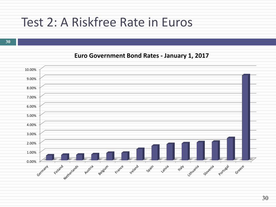
Test 2: A Riskfree Rate in Euros 30
0.00%
1.00%
2.00%
3.00%
4.00%
5.00%
6.00%
7.00%
8.00%
9.00%
10.00%
Euro Government Bond Rates - January 1, 2017
31
Test 3: A Riskfree Rate in Indian Rupees
The Indian government had 10-year Rupee bonds outstanding, with a yield to maturity of about 6.40% on January 1, 2017.
In January 2017, the Indian government had a local currency sovereign rating of Baa3. The typical default spread (over a default free rate) for Baa3 rated country bonds in early 2017 was 2.54%. The riskfree rate in Indian Rupees is a. The yield to maturity on the 10-year bond (6.40%)
b. The yield to maturity on the 10-year bond + Default spread (8.94%)
c. The yield to maturity on the 10-year bond – Default spread (3.86%)
d. None of the above
31
32
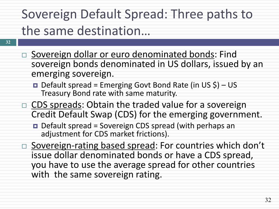
Sovereign Default Spread: Three paths to the same destination…
Sovereign dollar or euro denominated bonds: Find sovereign bonds denominated in US dollars, issued by an emerging sovereign. Default spread = Emerging Govt Bond Rate (in US $) – US
Treasury Bond rate with same maturity.
CDS spreads: Obtain the traded value for a sovereign Credit Default Swap (CDS) for the emerging government. Default spread = Sovereign CDS spread (with perhaps an
adjustment for CDS market frictions).
Sovereign-rating based spread: For countries which don’t issue dollar denominated bonds or have a CDS spread, you have to use the average spread for other countries with the same sovereign rating.
32
33
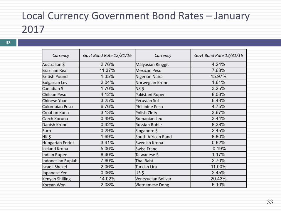
Local Currency Government Bond Rates – January 2017
33
Currency Govt Bond Rate 12/31/16 Currency Govt Bond Rate 12/31/16
Australian $ 2.76% Malyasian Ringgit 4.24%
Brazilian Reai 11.37% Mexican Peso 7.63%
British Pound 1.35% Nigerian Naira 15.97%
Bulgarian Lev 2.04% Norwegian Krone 1.61%
Canadian $ 1.70% NZ $ 3.25%
Chilean Peso 4.12% Pakistani Rupee 8.03%
Chinese Yuan 3.25% Peruvian Sol 6.43%
Colombian Peso 6.76% Phillipine Peso 4.75%
Croatian Kuna 3.13% Polish Zloty 3.67%
Czech Koruna 0.49% Romanian Leu 3.44%
Danish Krone 0.42% Russian Ruble 8.38%
Euro 0.29% Singapore $ 2.45%
HK $ 1.69% South African Rand 8.80%
Hungarian Forint 3.41% Swedish Krona 0.62%
Iceland Krona 5.06% Swiss Franc -0.19%
Indian Rupee 6.40% Taiwanese $ 1.17%
Indonesian Rupiah 7.60% Thai Baht 2.70%
Israeli Shekel 2.06% Turkish Lira 11.00%
Japanese Yen 0.06% US $ 2.45%
Kenyan Shilling 14.02% Venezuelan Bolivar 20.43%
Korean Won 2.08% Vietnamese Dong 6.10%
34
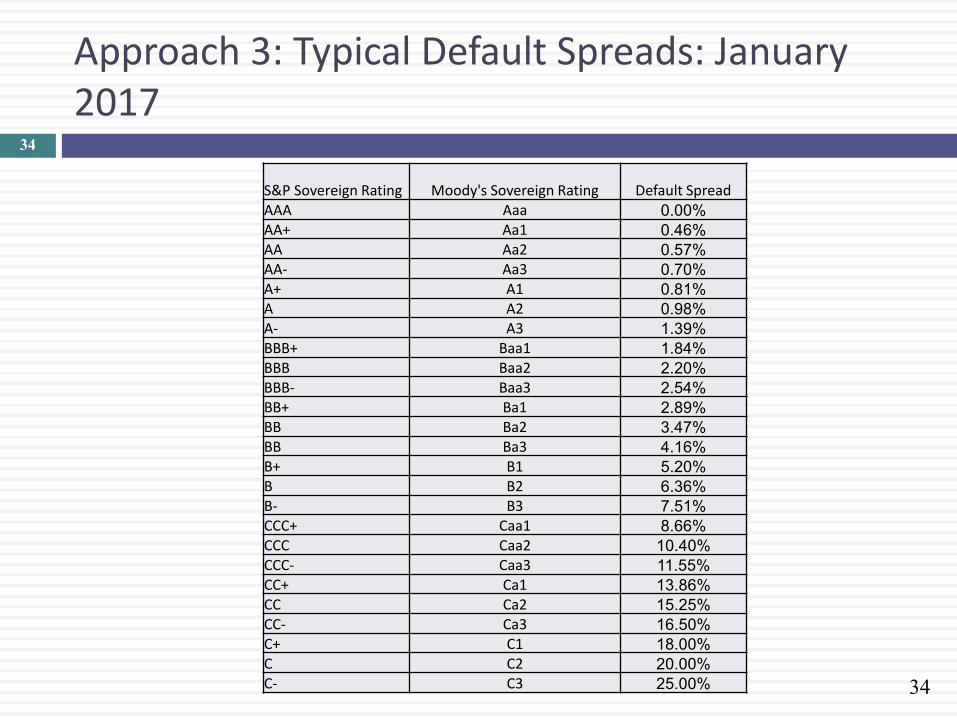
Approach 3: Typical Default Spreads: January 2017
34
S&P Sovereign Rating Moody's Sovereign Rating Default Spread AAA Aaa 0.00%
AA+ Aa1 0.46%
AA Aa2 0.57%
AA- Aa3 0.70%
A+ A1 0.81%
A A2 0.98%
A- A3 1.39%
BBB+ Baa1 1.84%
BBB Baa2 2.20%
BBB- Baa3 2.54%
BB+ Ba1 2.89%
BB Ba2 3.47%
BB Ba3 4.16%
B+ B1 5.20%
B B2 6.36%
B- B3 7.51%
CCC+ Caa1 8.66%
CCC Caa2 10.40%
CCC- Caa3 11.55%
CC+ Ca1 13.86%
CC Ca2 15.25%
CC- Ca3 16.50%
C+ C1 18.00%
C C2 20.00%
C- C3 25.00%
35
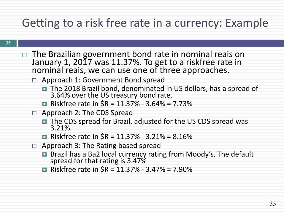
Getting to a risk free rate in a currency: Example
The Brazilian government bond rate in nominal reais on January 1, 2017 was 11.37%. To get to a riskfree rate in nominal reais, we can use one of three approaches. Approach 1: Government Bond spread The 2018 Brazil bond, denominated in US dollars, has a spread of
3.64% over the US treasury bond rate. Riskfree rate in $R = 11.37% - 3.64% = 7.73%
Approach 2: The CDS Spread The CDS spread for Brazil, adjusted for the US CDS spread was
3.21%. Riskfree rate in $R = 11.37% - 3.21% = 8.16%
Approach 3: The Rating based spread Brazil has a Ba2 local currency rating from Moody’s. The default
spread for that rating is 3.47% Riskfree rate in $R = 11.37% - 3.47% = 7.90%
35
36
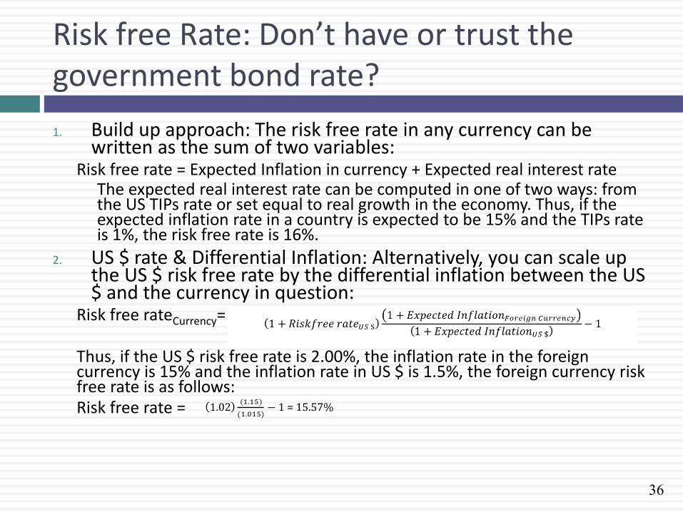
Risk free Rate: Don’t have or trust the government bond rate?
1. Build up approach: The risk free rate in any currency can be written as the sum of two variables:
Risk free rate = Expected Inflation in currency + Expected real interest rate The expected real interest rate can be computed in one of two ways: from the US TIPs rate or set equal to real growth in the economy. Thus, if the expected inflation rate in a country is expected to be 15% and the TIPs rate is 1%, the risk free rate is 16%.
2. US $ rate & Differential Inflation: Alternatively, you can scale up the US $ risk free rate by the differential inflation between the US $ and the currency in question:
Risk free rateCurrency= Thus, if the US $ risk free rate is 2.00%, the inflation rate in the foreign currency is 15% and the inflation rate in US $ is 1.5%, the foreign currency risk free rate is as follows: Risk free rate =

Aswath Damodaran 37

The Equity Risk Premium
Discount Rates: II 38

39
The ubiquitous historical risk premium
The historical premium is the premium that stocks have historically earned over riskless securities.
While the users of historical risk premiums act as if it is a fact (rather than an estimate), it is sensitive to
How far back you go in history…
Whether you use T.bill rates or T.Bond rates
Whether you use geometric or arithmetic averages.
For instance, looking at the US:
Aswath Damodaran
39
Arithmetic Average Geometric Average
Stocks - T. Bills Stocks - T. Bonds Stocks - T. Bills Stocks - T. Bonds 1928-2016 7.96% 6.24% 6.11% 4.62% Std Error 2.13% 2.28% 1967-2016 6.57% 4.37% 5.26% 3.42% Std Error 2.42% 2.74% 2007-2016 7.91% 3.62% 6.15% 2.30% Std Error 6.06% 8.66%

40
The perils of trusting the past…….
Noisy estimates: Even with long time periods of history, the risk premium that you derive will have substantial standard error. For instance, if you go back to 1928 (about 80 years of history) and you assume a standard deviation of 20% in annual stock returns, you arrive at a standard error of greater than 2%:
Standard Error in Premium = 20%/√80 = 2.26% Survivorship Bias: Using historical data from the U.S.
equity markets over the twentieth century does create a sampling bias. After all, the US economy and equity markets were among the most successful of the global economies that you could have invested in early in the century.
40

41
Risk Premium for a Mature Market? Broadening the sample to 1900-2015
41
Country Geometric ERP Arithmetic ERP Standard Error
Australia 5.00% 6.60% 1.70%
Austria 2.60% 21.50% 14.30%
Belgium 2.40% 4.50% 2.00%
Canada 3.30% 4.90% 1.70%
Denmark 2.30% 3.80% 1.70%
Finland 5.20% 8.80% 2.80%
France 3.00% 5.40% 2.10%
Germany 5.10% 9.10% 2.70%
Ireland 2.80% 4.80% 1.80%
Italy 3.10% 6.50% 2.70%
Japan 5.10% 9.10% 3.00%
Netherlands 3.30% 5.60% 2.10%
New Zealand 4.00% 5.50% 1.70%
Norway 2.30% 5.20% 2.60%
South Africa 5.40% 7.20% 1.80%
Spain 1.80% 3.80% 1.90%
Sweden 3.10% 5.40% 2.00%
Switzerland 2.10% 3.60% 1.60%
U.K. 3.60% 5.00% 1.60%
U.S. 4.30% 6.40% 1.90%
Europe 3.20% 4.50% 1.50%
World-ex U.S. 2.80% 3.90% 1.40%
World 3.20% 4.40% 1.40%
42
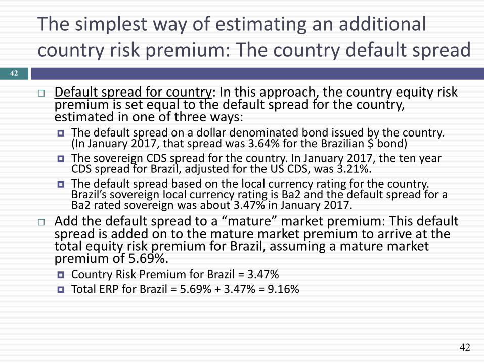
The simplest way of estimating an additional country risk premium: The country default spread
Default spread for country: In this approach, the country equity risk premium is set equal to the default spread for the country, estimated in one of three ways: The default spread on a dollar denominated bond issued by the country.
(In January 2017, that spread was 3.64% for the Brazilian $ bond) The sovereign CDS spread for the country. In January 2017, the ten year
CDS spread for Brazil, adjusted for the US CDS, was 3.21%. The default spread based on the local currency rating for the country.
Brazil’s sovereign local currency rating is Ba2 and the default spread for a Ba2 rated sovereign was about 3.47% in January 2017.
Add the default spread to a “mature” market premium: This default spread is added on to the mature market premium to arrive at the total equity risk premium for Brazil, assuming a mature market premium of 5.69%. Country Risk Premium for Brazil = 3.47% Total ERP for Brazil = 5.69% + 3.47% = 9.16%
42

43
An equity volatility based approach to estimating the country total ERP
This approach draws on the standard deviation of two equity markets, the emerging market in question and a base market (usually the US). The total equity risk premium for the emerging market is then written as: Total equity risk premium = Risk PremiumUS* Country Equity / US Equity
The country equity risk premium is based upon the volatility of the market in question relative to U.S market. Assume that the equity risk premium for the US is 5.69%.
Assume that the standard deviation in the Bovespa (Brazilian equity) is 30% and that the standard deviation for the S&P 500 (US equity) is 18%.
Total Equity Risk Premium for Brazil = 5.69% (30%/18%) = 9.48%
Country equity risk premium for Brazil = 9.48% - 5.69% = 3.79%
43
44
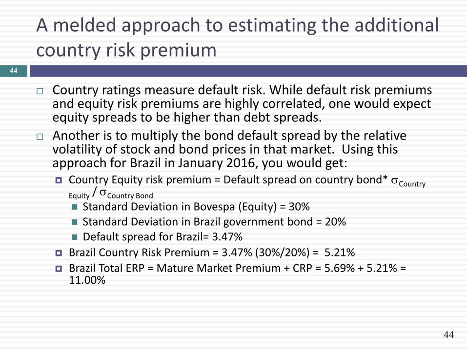
A melded approach to estimating the additional country risk premium
Country ratings measure default risk. While default risk premiums and equity risk premiums are highly correlated, one would expect equity spreads to be higher than debt spreads.
Another is to multiply the bond default spread by the relative volatility of stock and bond prices in that market. Using this approach for Brazil in January 2016, you would get: Country Equity risk premium = Default spread on country bond* Country
Equity / Country Bond
Standard Deviation in Bovespa (Equity) = 30% Standard Deviation in Brazil government bond = 20% Default spread for Brazil= 3.47%
Brazil Country Risk Premium = 3.47% (30%/20%) = 5.21%
Brazil Total ERP = Mature Market Premium + CRP = 5.69% + 5.21% = 11.00%
44
45
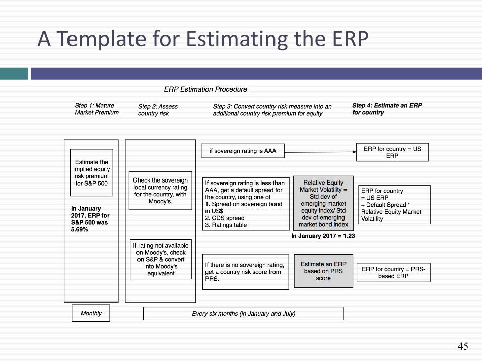
A Template for Estimating the ERP
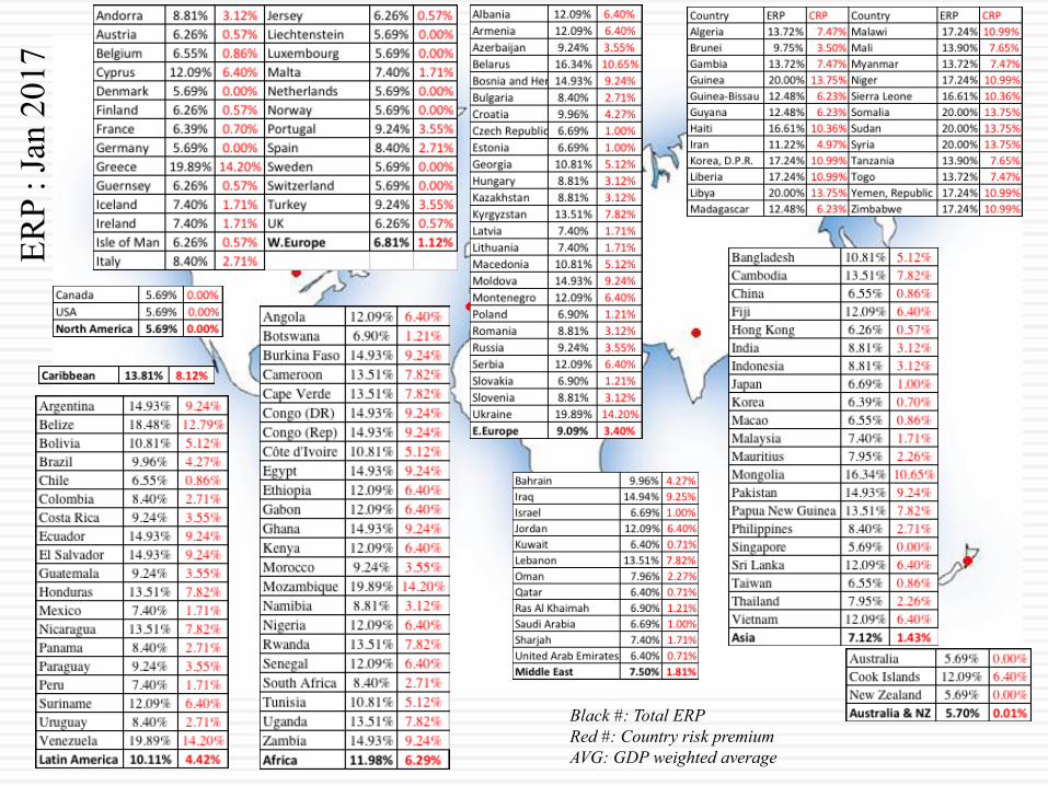
Black #: Total ERP
Red #: Country risk premium
AVG: GDP weighted average
ER
P :
Jan
2017
47
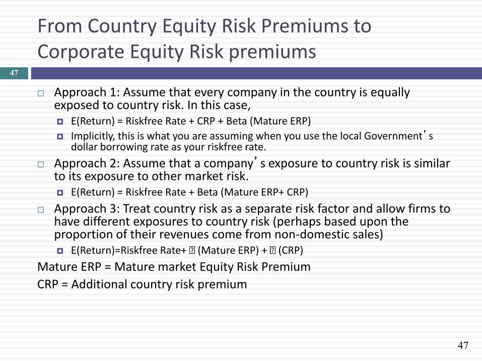
From Country Equity Risk Premiums to Corporate Equity Risk premiums
Approach 1: Assume that every company in the country is equally exposed to country risk. In this case, E(Return) = Riskfree Rate + CRP + Beta (Mature ERP)
Implicitly, this is what you are assuming when you use the local Government’s dollar borrowing rate as your riskfree rate.
Approach 2: Assume that a company’s exposure to country risk is similar to its exposure to other market risk. E(Return) = Riskfree Rate + Beta (Mature ERP+ CRP)
Approach 3: Treat country risk as a separate risk factor and allow firms to have different exposures to country risk (perhaps based upon the proportion of their revenues come from non-domestic sales) E(Return)=Riskfree Rate+ (Mature ERP) + (CRP)
Mature ERP = Mature market Equity Risk Premium
CRP = Additional country risk premium
47
48
Approaches 1 & 2: Estimating country risk premium exposure
Location based CRP: The standard approach in valuation is to attach a country risk premium to a company based upon its country of incorporation. Thus, if you are an Indian company, you are assumed to be exposed to the Indian country risk premium. A developed market company is assumed to be unexposed to emerging market risk.
Operation-based CRP: There is a more reasonable modified version. The country risk premium for a company can be computed as a weighted average of the country risk premiums of the countries that it does business in, with the weights based upon revenues or operating income. If a company is exposed to risk in dozens of countries, you can take a weighted average of the risk premiums by region.
48
49
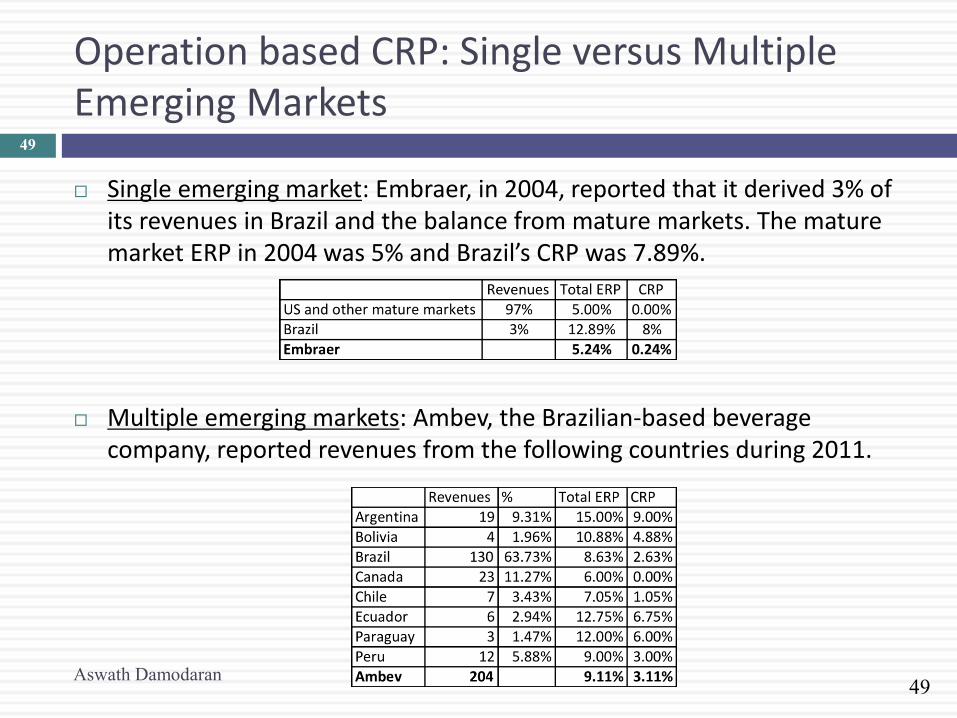
Operation based CRP: Single versus Multiple Emerging Markets
Single emerging market: Embraer, in 2004, reported that it derived 3% of its revenues in Brazil and the balance from mature markets. The mature market ERP in 2004 was 5% and Brazil’s CRP was 7.89%.
Multiple emerging markets: Ambev, the Brazilian-based beverage company, reported revenues from the following countries during 2011.
Aswath Damodaran
49

50
Extending to a multinational: Regional breakdown Coca Cola’s revenue breakdown and ERP in 2012
Things to watch out for
1. Aggregation across regions. For instance, the Pacific region often includes Australia & NZ with Asia
2. Obscure aggregations including Eurasia and Oceania
50
51
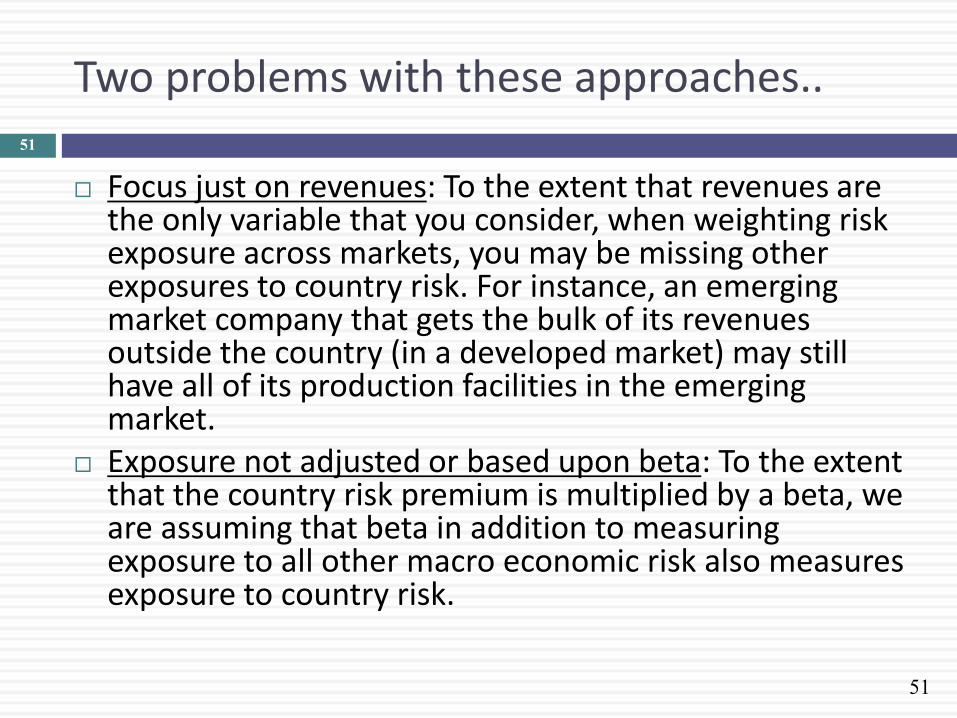
Two problems with these approaches..
Focus just on revenues: To the extent that revenues are the only variable that you consider, when weighting risk exposure across markets, you may be missing other exposures to country risk. For instance, an emerging market company that gets the bulk of its revenues outside the country (in a developed market) may still have all of its production facilities in the emerging market.
Exposure not adjusted or based upon beta: To the extent that the country risk premium is multiplied by a beta, we are assuming that beta in addition to measuring exposure to all other macro economic risk also measures exposure to country risk.
51
52
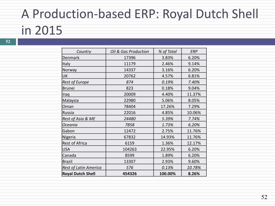
A Production-based ERP: Royal Dutch Shell in 2015
52
Country Oil & Gas Production % of Total ERP
Denmark 17396 3.83% 6.20%
Italy 11179 2.46% 9.14%
Norway 14337 3.16% 6.20%
UK 20762 4.57% 6.81%
Rest of Europe 874 0.19% 7.40%
Brunei 823 0.18% 9.04%
Iraq 20009 4.40% 11.37%
Malaysia 22980 5.06% 8.05%
Oman 78404 17.26% 7.29%
Russia 22016 4.85% 10.06%
Rest of Asia & ME 24480 5.39% 7.74%
Oceania 7858 1.73% 6.20%
Gabon 12472 2.75% 11.76%
Nigeria 67832 14.93% 11.76%
Rest of Africa 6159 1.36% 12.17%
USA 104263 22.95% 6.20%
Canada 8599 1.89% 6.20%
Brazil 13307 2.93% 9.60%
Rest of Latin America 576 0.13% 10.78%
Royal Dutch Shell 454326 100.00% 8.26%
53
Approach 3: Estimate a lambda for country risk
Country risk exposure is affected by where you get your revenues and where your production happens, but there are a host of other variables that also affect this exposure, including: Use of risk management products: Companies can use both options/futures
markets and insurance to hedge some or a significant portion of country risk.
Government “national” interests: There are sectors that are viewed as vital to the national interests, and governments often play a key role in these companies, either officially or unofficially. These sectors are more exposed to country risk.
It is conceivable that there is a richer measure of country risk that incorporates all of the variables that drive country risk in one measure. That way my rationale when I devised “lambda” as my measure of country risk exposure.
53

54
A Revenue-based Lambda
The factor “l” measures the relative exposure of a firm to country risk. One simplistic solution would be to do the following: l = % of revenues domesticallyfirm/ % of revenues domesticallyaverage firm
Consider two firms – Tata Motors and Tata Consulting Services, both Indian companies. In 2008-09, Tata Motors got about 91.37% of its revenues in India and TCS got 7.62%. The average Indian firm gets about 80% of its revenues in India: l Tata Motors= 91%/80% = 1.14
l TCS= 7.62%/80% = 0.09
There are two implications A company’s risk exposure is determined by where it does business and
not by where it is incorporated.
Firms might be able to actively manage their country risk exposures
55
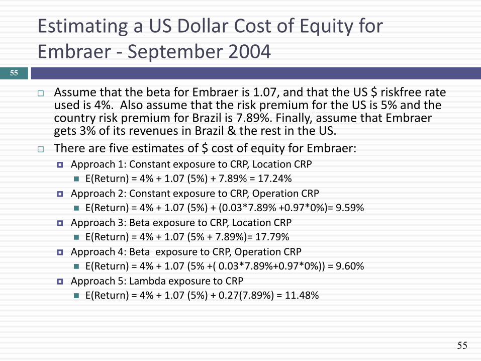
Estimating a US Dollar Cost of Equity for Embraer - September 2004
Assume that the beta for Embraer is 1.07, and that the US $ riskfree rate used is 4%. Also assume that the risk premium for the US is 5% and the country risk premium for Brazil is 7.89%. Finally, assume that Embraer gets 3% of its revenues in Brazil & the rest in the US.
There are five estimates of $ cost of equity for Embraer: Approach 1: Constant exposure to CRP, Location CRP
E(Return) = 4% + 1.07 (5%) + 7.89% = 17.24%
Approach 2: Constant exposure to CRP, Operation CRP
E(Return) = 4% + 1.07 (5%) + (0.03*7.89% +0.97*0%)= 9.59%
Approach 3: Beta exposure to CRP, Location CRP E(Return) = 4% + 1.07 (5% + 7.89%)= 17.79%
Approach 4: Beta exposure to CRP, Operation CRP
E(Return) = 4% + 1.07 (5% +( 0.03*7.89%+0.97*0%)) = 9.60%
Approach 5: Lambda exposure to CRP
E(Return) = 4% + 1.07 (5%) + 0.27(7.89%) = 11.48%
55
56
Valuing Emerging Market Companies with significant exposure in developed markets
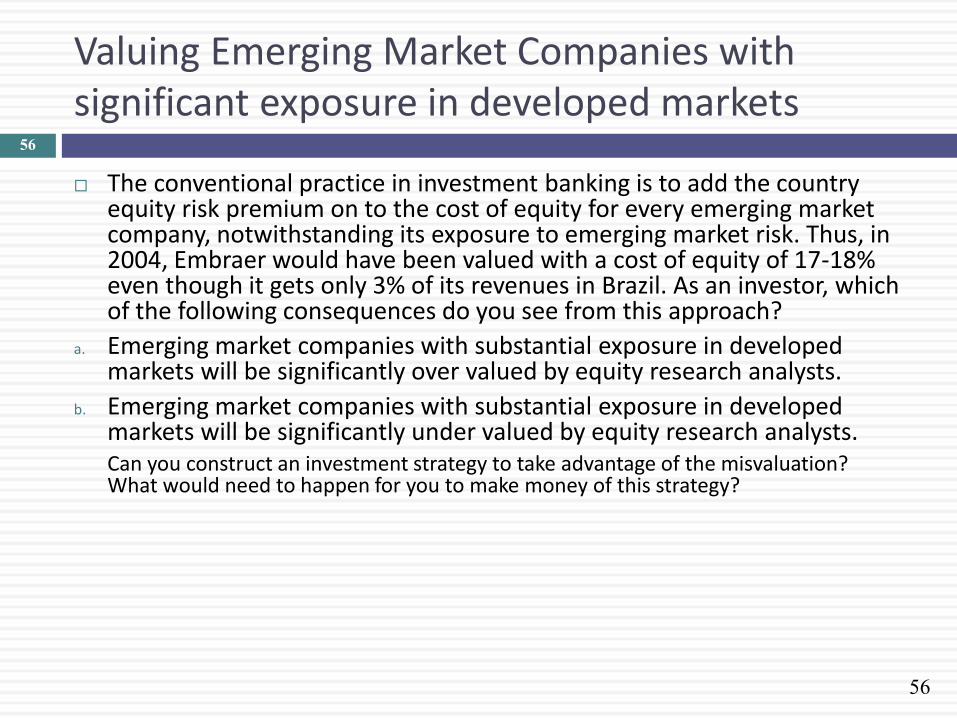
The conventional practice in investment banking is to add the country equity risk premium on to the cost of equity for every emerging market company, notwithstanding its exposure to emerging market risk. Thus, in 2004, Embraer would have been valued with a cost of equity of 17-18% even though it gets only 3% of its revenues in Brazil. As an investor, which of the following consequences do you see from this approach?
a. Emerging market companies with substantial exposure in developed markets will be significantly over valued by equity research analysts.
b. Emerging market companies with substantial exposure in developed markets will be significantly under valued by equity research analysts. Can you construct an investment strategy to take advantage of the misvaluation? What would need to happen for you to make money of this strategy?
56

57
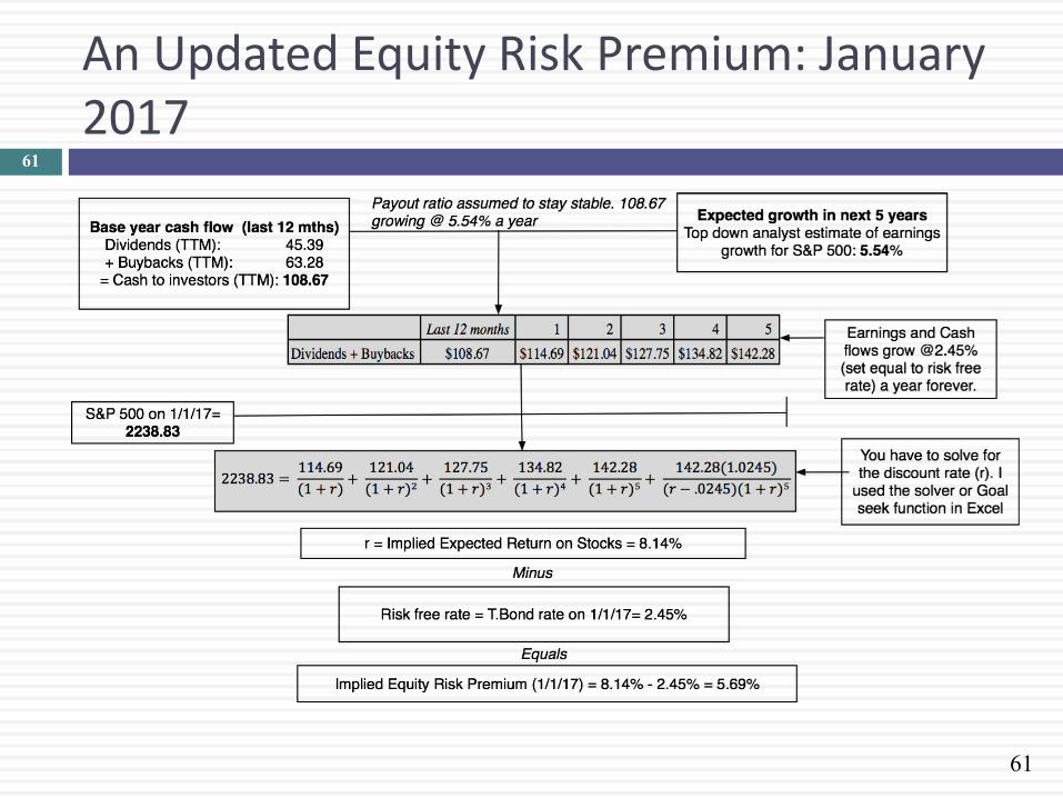
Implied Equity Premiums
Let’s start with a general proposition. If you know the price paid for an asset and have estimates of the expected cash flows on the asset, you can estimate the IRR of these cash flows. If you paid the price, this is what you have priced the asset to earn (as an expected return).
If you assume that stocks are correctly priced in the aggregate and you can estimate the expected cashflows from buying stocks, you can estimate the expected rate of return on stocks by finding that discount rate that makes the present value equal to the price paid. Subtracting out the riskfree rate should yield an implied equity risk premium.
This implied equity premium is a forward looking number and can be updated as often as you want (every minute of every day, if you are so inclined).
57
58
Implied Equity Premiums: January 2008
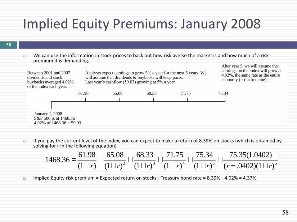
We can use the information in stock prices to back out how risk averse the market is and how much of a risk premium it is demanding.
If you pay the current level of the index, you can expect to make a return of 8.39% on stocks (which is obtained by solving for r in the following equation)
Implied Equity risk premium = Expected return on stocks - Treasury bond rate = 8.39% - 4.02% = 4.37%
1468.36 =61.98
(1+ r)+
65.08
(1+ r)2+
68.33
(1+ r)3+
71.75
(1+ r)4+
75.34
(1+ r)5+
75.35(1.0402)
(r - .0402)(1+ r)5
January 1, 2008S&P 500 is at 1468.364.02% of 1468.36 = 59.03
Between 2001 and 2007 dividends and stock buybacks averaged 4.02% of the index each year.
Analysts expect earnings to grow 5% a year for the next 5 years. We will assume that dividends & buybacks will keep pace..Last year’s cashflow (59.03) growing at 5% a year
After year 5, we will assume that earnings on the index will grow at 4.02%, the same rate as the entire economy (= riskfree rate).
61.98 65.08 68.33 71.75 75.34
58
59
A year that made a difference.. The implied premium in January 2009
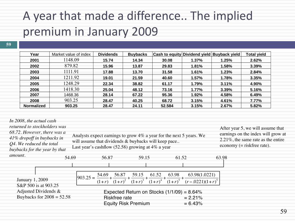
Year Market value of index Dividends Buybacks Cash to equity Dividend yield Buyback yield Total yield
2001 1148.09 15.74 14.34 30.08 1.37% 1.25% 2.62%
2002 879.82 15.96 13.87 29.83 1.81% 1.58% 3.39%
2003 1111.91 17.88 13.70 31.58 1.61% 1.23% 2.84%
2004 1211.92 19.01 21.59 40.60 1.57% 1.78% 3.35%
2005 1248.29 22.34 38.82 61.17 1.79% 3.11% 4.90%
2006 1418.30 25.04 48.12 73.16 1.77% 3.39% 5.16%
2007 1468.36 28.14 67.22 95.36 1.92% 4.58% 6.49%
2008 903.25 28.47 40.25 68.72 3.15% 4.61% 7.77%
Normalized 903.25 28.47 24.11 52.584 3.15% 2.67% 5.82%
59
60
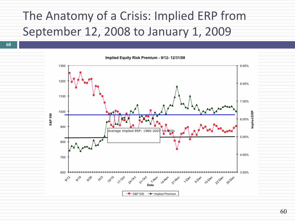
The Anatomy of a Crisis: Implied ERP from September 12, 2008 to January 1, 2009
60
61
An Updated Equity Risk Premium: January 2017
61

Aswath Damodaran 62
63
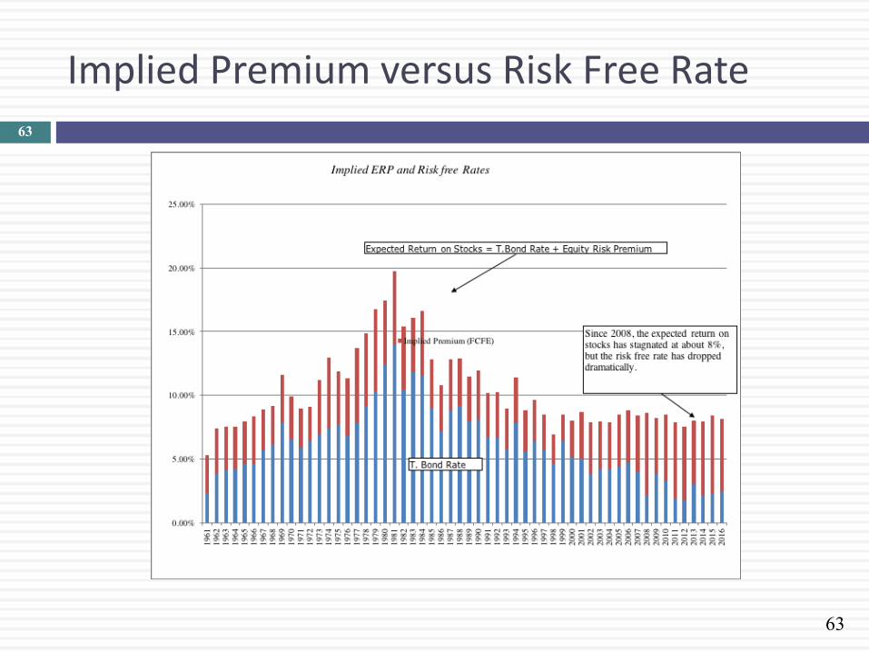
Implied Premium versus Risk Free Rate 63
64
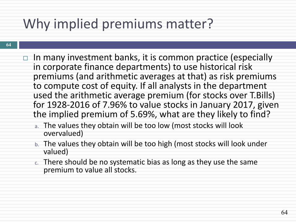
Why implied premiums matter?
In many investment banks, it is common practice (especially in corporate finance departments) to use historical risk premiums (and arithmetic averages at that) as risk premiums to compute cost of equity. If all analysts in the department used the arithmetic average premium (for stocks over T.Bills) for 1928-2016 of 7.96% to value stocks in January 2017, given the implied premium of 5.69%, what are they likely to find? a. The values they obtain will be too low (most stocks will look
overvalued)
b. The values they obtain will be too high (most stocks will look under valued)
c. There should be no systematic bias as long as they use the same premium to value all stocks.
64
65
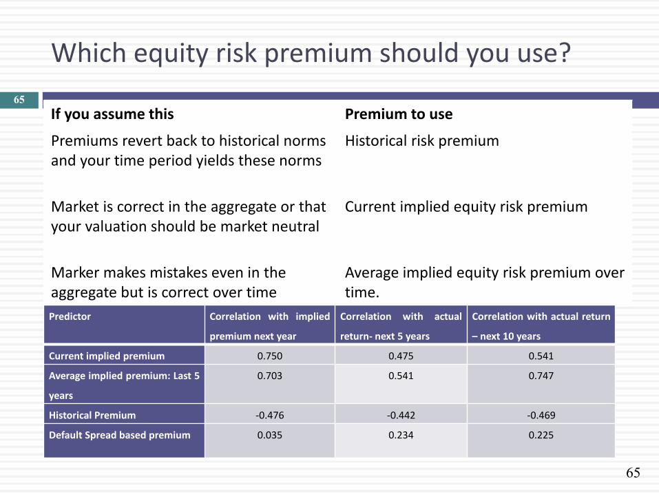
Which equity risk premium should you use?
If you assume this Premium to use
Premiums revert back to historical norms and your time period yields these norms
Historical risk premium
Market is correct in the aggregate or that your valuation should be market neutral
Current implied equity risk premium
Marker makes mistakes even in the aggregate but is correct over time
Average implied equity risk premium over time.
65
Predictor Correlation with implied
premium next year
Correlation with actual
return- next 5 years
Correlation with actual return
– next 10 years
Current implied premium 0.750 0.475 0.541
Average implied premium: Last 5
years
0.703 0.541 0.747
Historical Premium -0.476 -0.442 -0.469
Default Spread based premium 0.035 0.234 0.225

66
An ERP for the Kuwait
Inputs for the computation KSE VW Index on 27/9/17 = 429.74
Dividend yield on index = 4.37%
Expected growth rate - next 5 years = 7.5%
Growth rate beyond year 5 = 2.25% (set equal to riskfree rate)
Solving for the expected return:
Expected return on stocks = 7.86% Implied equity risk premium for India = 7.86% - 2.25% =
5.61%
66
429.74 =20.19
1 + 𝑟+
21.70
1 + 𝑟 2+
23.33
1 + 𝑟 3+
25.08
1 + 𝑟 4+
26.95
1 + 𝑟 5+
26.95(1 + 0.025
𝑟 − 0.025 (1 + 𝑟 5
67
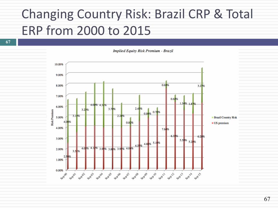
Changing Country Risk: Brazil CRP & Total ERP from 2000 to 2015
67
68
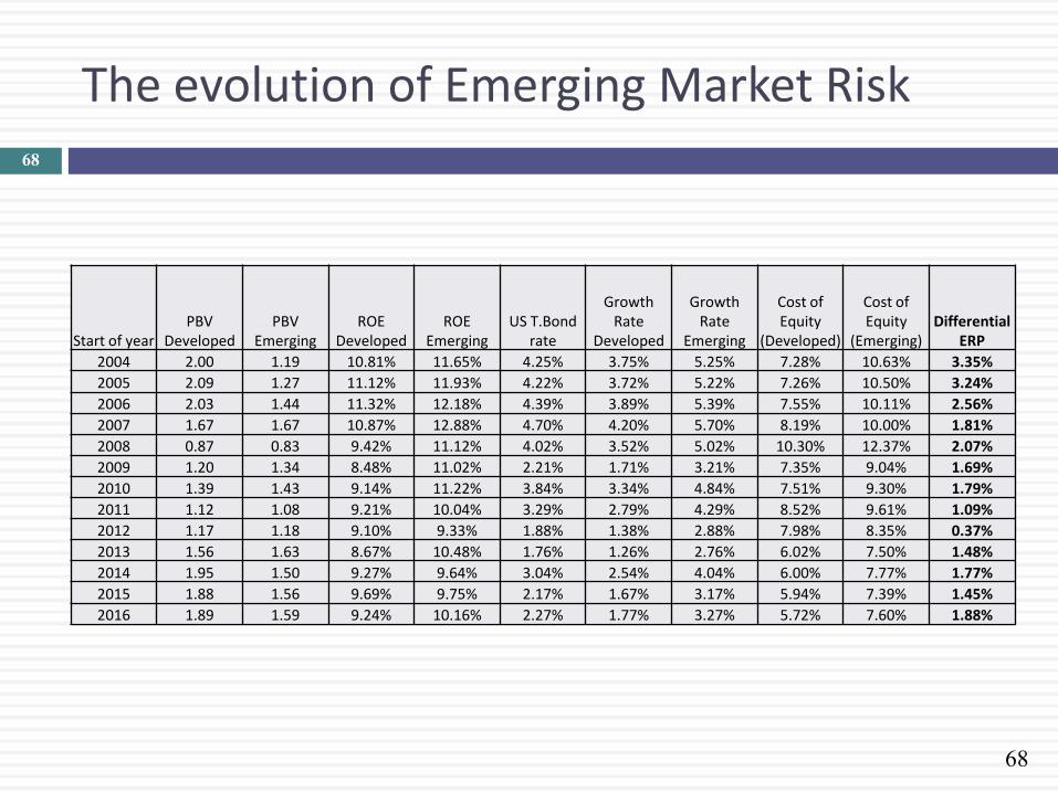
The evolution of Emerging Market Risk 68
Start of year PBV
Developed PBV
Emerging ROE
Developed ROE
Emerging US T.Bond
rate
Growth Rate
Developed
Growth Rate
Emerging
Cost of Equity
(Developed)
Cost of Equity
(Emerging) Differential
ERP
2004 2.00 1.19 10.81% 11.65% 4.25% 3.75% 5.25% 7.28% 10.63% 3.35%
2005 2.09 1.27 11.12% 11.93% 4.22% 3.72% 5.22% 7.26% 10.50% 3.24%
2006 2.03 1.44 11.32% 12.18% 4.39% 3.89% 5.39% 7.55% 10.11% 2.56%
2007 1.67 1.67 10.87% 12.88% 4.70% 4.20% 5.70% 8.19% 10.00% 1.81%
2008 0.87 0.83 9.42% 11.12% 4.02% 3.52% 5.02% 10.30% 12.37% 2.07%
2009 1.20 1.34 8.48% 11.02% 2.21% 1.71% 3.21% 7.35% 9.04% 1.69%
2010 1.39 1.43 9.14% 11.22% 3.84% 3.34% 4.84% 7.51% 9.30% 1.79%
2011 1.12 1.08 9.21% 10.04% 3.29% 2.79% 4.29% 8.52% 9.61% 1.09%
2012 1.17 1.18 9.10% 9.33% 1.88% 1.38% 2.88% 7.98% 8.35% 0.37%
2013 1.56 1.63 8.67% 10.48% 1.76% 1.26% 2.76% 6.02% 7.50% 1.48%
2014 1.95 1.50 9.27% 9.64% 3.04% 2.54% 4.04% 6.00% 7.77% 1.77%
2015 1.88 1.56 9.69% 9.75% 2.17% 1.67% 3.17% 5.94% 7.39% 1.45%
2016 1.89 1.59 9.24% 10.16% 2.27% 1.77% 3.27% 5.72% 7.60% 1.88%
Relative Risk Measures
Discount Rates: III 69

70
The CAPM Beta: The Most Used (and Misused) Risk Measure
The standard procedure for estimating betas is to regress stock returns (Rj) against market returns (Rm) - Rj = a + b Rm where a is the intercept and b is the slope of the regression.
The slope of the regression corresponds to the beta of the stock, and measures the riskiness of the stock.
This beta has three problems: • It has high standard error • It reflects the firm’s business mix over the period of the
regression, not the current mix • It reflects the firm’s average financial leverage over the period
rather than the current leverage.
70

71
Unreliable, when it looks bad.. 71
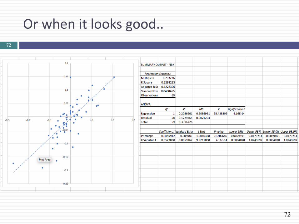
72
Or when it looks good.. 72
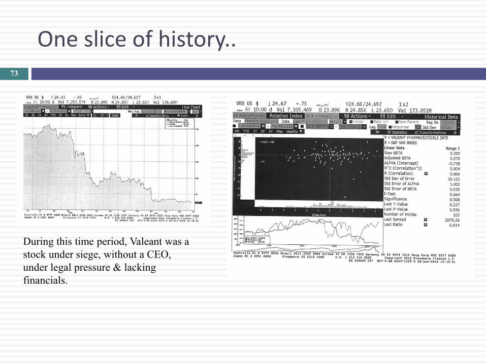
One slice of history.. 73
During this time period, Valeant was a
stock under siege, without a CEO,
under legal pressure & lacking
financials.
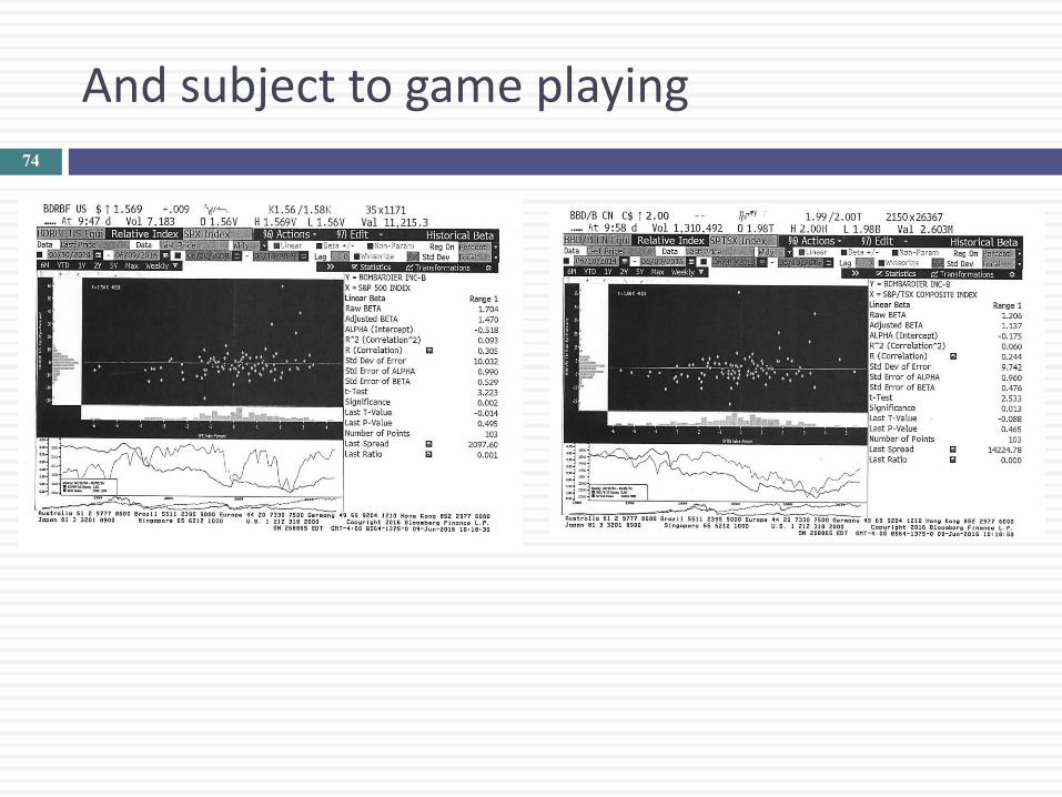
And subject to game playing 74
75
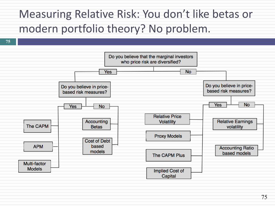
Measuring Relative Risk: You don’t like betas or modern portfolio theory? No problem.
75
76
Don’t like the diversified investor focus, but okay with price-based measures
1. Relative Standard Deviation • Relative Volatility = Std dev of Stock/ Average Std dev across all stocks • Captures all risk, rather than just market risk
2. Proxy Models • Look at historical returns on all stocks and look for variables that
explain differences in returns. • You are, in effect, running multiple regressions with returns on
individual stocks as the dependent variable and fundamentals about these stocks as independent variables.
• This approach started with market cap (the small cap effect) and over the last two decades has added other variables (momentum, liquidity etc.)
3. CAPM Plus Models • Start with the traditional CAPM (Rf + Beta (ERP)) and then add other
premiums for proxies.
76
77
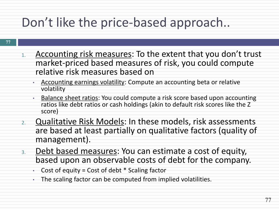
Don’t like the price-based approach..
1. Accounting risk measures: To the extent that you don’t trust market-priced based measures of risk, you could compute relative risk measures based on
• Accounting earnings volatility: Compute an accounting beta or relative volatility
• Balance sheet ratios: You could compute a risk score based upon accounting ratios like debt ratios or cash holdings (akin to default risk scores like the Z score)
2. Qualitative Risk Models: In these models, risk assessments are based at least partially on qualitative factors (quality of management).
3. Debt based measures: You can estimate a cost of equity, based upon an observable costs of debt for the company.
• Cost of equity = Cost of debt * Scaling factor
• The scaling factor can be computed from implied volatilities.
77

78
Determinants of Betas & Relative Risk 78
79
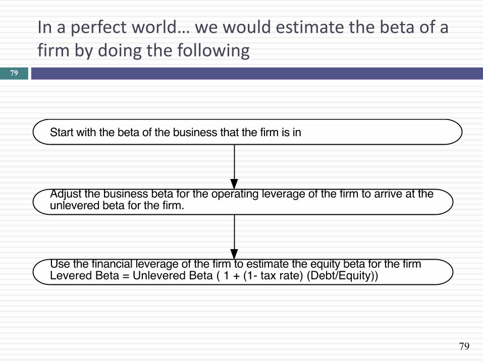
In a perfect world… we would estimate the beta of a firm by doing the following
79
80
Adjusting for operating leverage…
Within any business, firms with lower fixed costs (as a percentage of total costs) should have lower unlevered betas. If you can compute fixed and variable costs for each firm in a sector, you can break down the unlevered beta into business and operating leverage components. Unlevered beta = Pure business beta * (1 + (Fixed costs/ Variable
costs))
The biggest problem with doing this is informational. It is difficult to get information on fixed and variable costs for individual firms.
In practice, we tend to assume that the operating leverage of firms within a business are similar and use the same unlevered beta for every firm.
80

81
Adjusting for financial leverage…
Conventional approach: If we assume that debt carries no market risk (has a beta of zero), the beta of equity alone can be written as a function of the unlevered beta and the debt-equity ratio bL = bu (1+ ((1-t)D/E)) In some versions, the tax effect is ignored and there is no (1-t) in the equation.
Debt Adjusted Approach: If beta carries market risk and you can estimate the beta of debt, you can estimate the levered beta as follows: bL = bu (1+ ((1-t)D/E)) - bdebt (1-t) (D/E) While the latter is more realistic, estimating betas for debt can be difficult to do.
81
82
Bottom-up Betas 82

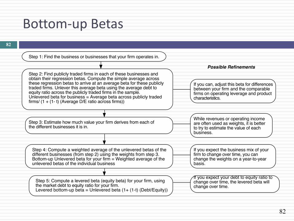
83
Why bottom-up betas?
The standard error in a bottom-up beta will be significantly lower than the standard error in a single regression beta. Roughly speaking, the standard error of a bottom-up beta estimate can be written as follows:
Std error of bottom-up beta =
The bottom-up beta can be adjusted to reflect changes in the firm’s business mix and financial leverage. Regression betas reflect the past.
You can estimate bottom-up betas even when you do not have historical stock prices. This is the case with initial public offerings, private businesses or divisions of companies.
Average Std Error across Betas
Number of firms in sample
83
84
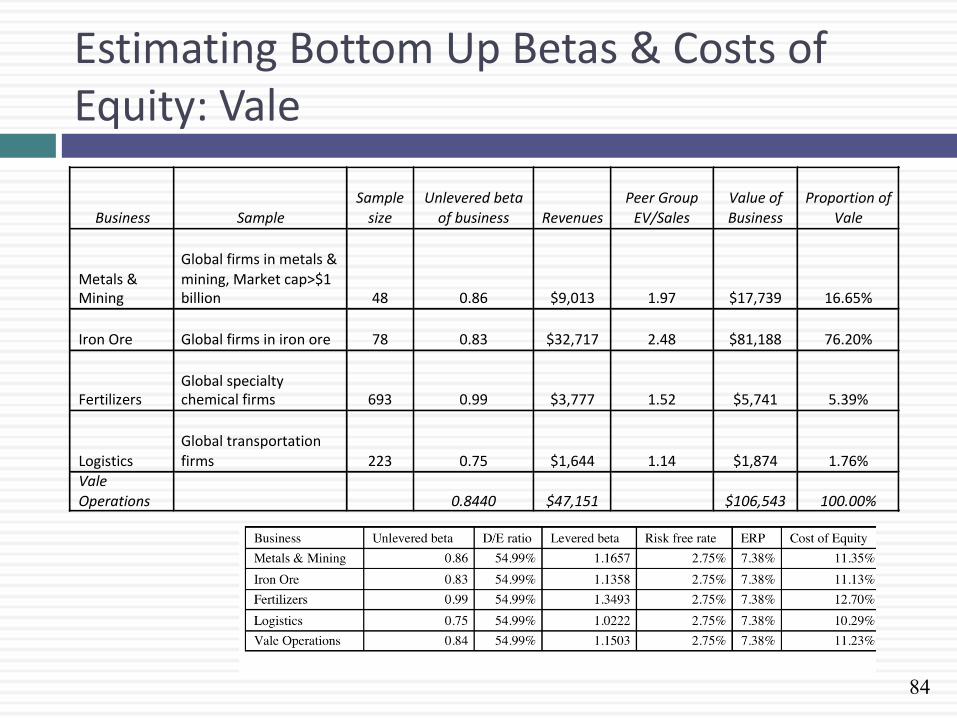
Estimating Bottom Up Betas & Costs of Equity: Vale
Business Sample
Sample
size
Unleveredbeta
ofbusiness Revenues
PeerGroup
EV/Sales
Valueof
Business
Proportionof
Vale
Metals&Mining
Globalfirmsinmetals&
mining,Marketcap>$1billion 48 0.86 $9,013 1.97 $17,739 16.65%
IronOre Globalfirmsinironore 78 0.83 $32,717 2.48 $81,188 76.20%
FertilizersGlobalspecialtychemicalfirms 693 0.99 $3,777 1.52 $5,741 5.39%
LogisticsGlobaltransportationfirms 223 0.75 $1,644 1.14 $1,874 1.76%
ValeOperations 0.8440 $47,151 $106,543 100.00%

85
Embraer’s Bottom-up Beta
Business Unlevered Beta D/E Ratio Levered beta
Aerospace 0.95 18.95% 1.07
Levered Beta = Unlevered Beta ( 1 + (1- tax rate) (D/E Ratio)
= 0.95 ( 1 + (1-.34) (.1895)) = 1.07
Can an unlevered beta estimated using U.S. and European aerospace companies be used to estimate the beta for a Brazilian aerospace company?
a. Yes
b. No What concerns would you have in making this assumption?
85

86
Gross Debt versus Net Debt Approaches
Analysts in Europe and Latin America often take the difference between debt and cash (net debt) when computing debt ratios and arrive at very different values.
For Embraer, using the gross debt ratio Gross D/E Ratio for Embraer = 1953/11,042 = 18.95%
Levered Beta using Gross Debt ratio = 1.07
Using the net debt ratio, we get Net Debt Ratio for Embraer = (Debt - Cash)/ Market value of Equity
= (1953-2320)/ 11,042 = -3.32%
Levered Beta using Net Debt Ratio = 0.95 (1 + (1-.34) (-.0332)) = 0.93
The cost of Equity using net debt levered beta for Embraer will be much lower than with the gross debt approach. The cost of capital for Embraer will even out since the debt ratio used in the cost of capital equation will now be a net debt ratio rather than a gross debt ratio.
86
87
The Cost of Equity: A Recap 87
Mopping up
Discount Rates: IV 88

89
Estimating the Cost of Debt
The cost of debt is the rate at which you can borrow at currently, It will reflect not only your default risk but also the level of interest rates in the market.
The two most widely used approaches to estimating cost of debt are: Looking up the yield to maturity on a straight bond outstanding from
the firm. The limitation of this approach is that very few firms have long term straight bonds that are liquid and widely traded
Looking up the rating for the firm and estimating a default spread based upon the rating. While this approach is more robust, different bonds from the same firm can have different ratings. You have to use a median rating for the firm
When in trouble (either because you have no ratings or multiple ratings for a firm), estimate a synthetic rating for your firm and the cost of debt based upon that rating.
89

90
Estimating Synthetic Ratings
The rating for a firm can be estimated using the financial characteristics of the firm. In its simplest form, the rating can be estimated from the interest coverage ratio
Interest Coverage Ratio = EBIT / Interest Expenses
For Embraer’s interest coverage ratio, we used the interest expenses from 2003 and the average EBIT from 2001 to 2003. (The aircraft business was badly affected by 9/11 and its aftermath. In 2002 and 2003, Embraer reported significant drops in operating income)
Interest Coverage Ratio = 462.1 /129.70 = 3.56
90
91
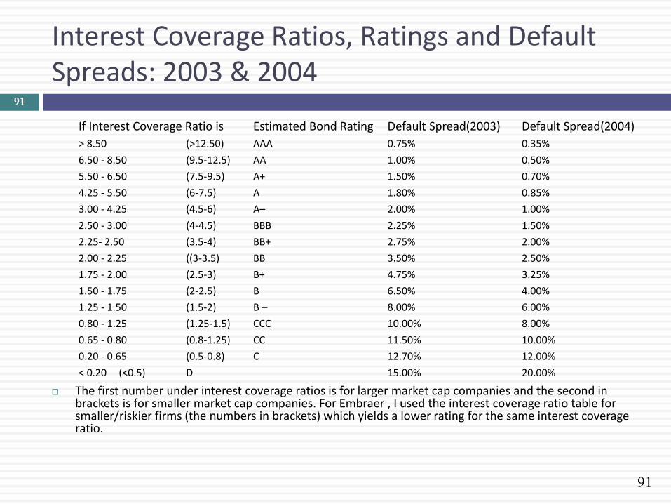
Interest Coverage Ratios, Ratings and Default Spreads: 2003 & 2004
If Interest Coverage Ratio is Estimated Bond Rating Default Spread(2003) Default Spread(2004)
> 8.50 (>12.50) AAA 0.75% 0.35%
6.50 - 8.50 (9.5-12.5) AA 1.00% 0.50%
5.50 - 6.50 (7.5-9.5) A+ 1.50% 0.70%
4.25 - 5.50 (6-7.5) A 1.80% 0.85%
3.00 - 4.25 (4.5-6) A– 2.00% 1.00%
2.50 - 3.00 (4-4.5) BBB 2.25% 1.50%
2.25- 2.50 (3.5-4) BB+ 2.75% 2.00%
2.00 - 2.25 ((3-3.5) BB 3.50% 2.50%
1.75 - 2.00 (2.5-3) B+ 4.75% 3.25%
1.50 - 1.75 (2-2.5) B 6.50% 4.00%
1.25 - 1.50 (1.5-2) B – 8.00% 6.00%
0.80 - 1.25 (1.25-1.5) CCC 10.00% 8.00%
0.65 - 0.80 (0.8-1.25) CC 11.50% 10.00%
0.20 - 0.65 (0.5-0.8) C 12.70% 12.00%
< 0.20 (<0.5) D 15.00% 20.00%
The first number under interest coverage ratios is for larger market cap companies and the second in brackets is for smaller market cap companies. For Embraer , I used the interest coverage ratio table for smaller/riskier firms (the numbers in brackets) which yields a lower rating for the same interest coverage ratio.
91
92
Cost of Debt computations
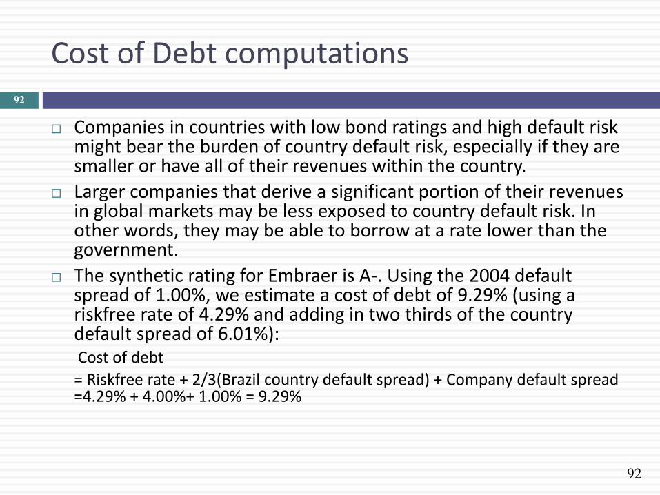
Companies in countries with low bond ratings and high default risk might bear the burden of country default risk, especially if they are smaller or have all of their revenues within the country.
Larger companies that derive a significant portion of their revenues in global markets may be less exposed to country default risk. In other words, they may be able to borrow at a rate lower than the government.
The synthetic rating for Embraer is A-. Using the 2004 default spread of 1.00%, we estimate a cost of debt of 9.29% (using a riskfree rate of 4.29% and adding in two thirds of the country default spread of 6.01%): Cost of debt
= Riskfree rate + 2/3(Brazil country default spread) + Company default spread =4.29% + 4.00%+ 1.00% = 9.29%
92
93
Synthetic Ratings: Some Caveats
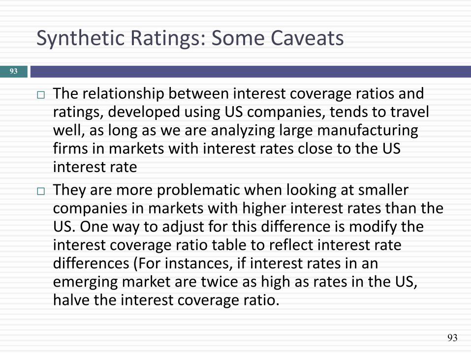
The relationship between interest coverage ratios and ratings, developed using US companies, tends to travel well, as long as we are analyzing large manufacturing firms in markets with interest rates close to the US interest rate
They are more problematic when looking at smaller companies in markets with higher interest rates than the US. One way to adjust for this difference is modify the interest coverage ratio table to reflect interest rate differences (For instances, if interest rates in an emerging market are twice as high as rates in the US, halve the interest coverage ratio.
93

94
Default Spreads: The effect of the crisis of 2008.. And the aftermath
Default spread over treasury
Rating 1-Jan-08 12-Sep-08 12-Nov-08 1-Jan-09 1-Jan-10 1-Jan-11
Aaa/AAA 0.99% 1.40% 2.15% 2.00% 0.50% 0.55%
Aa1/AA+ 1.15% 1.45% 2.30% 2.25% 0.55% 0.60%
Aa2/AA 1.25% 1.50% 2.55% 2.50% 0.65% 0.65%
Aa3/AA- 1.30% 1.65% 2.80% 2.75% 0.70% 0.75%
A1/A+ 1.35% 1.85% 3.25% 3.25% 0.85% 0.85%
A2/A 1.42% 1.95% 3.50% 3.50% 0.90% 0.90%
A3/A- 1.48% 2.15% 3.75% 3.75% 1.05% 1.00%
Baa1/BBB+ 1.73% 2.65% 4.50% 5.25% 1.65% 1.40%
Baa2/BBB 2.02% 2.90% 5.00% 5.75% 1.80% 1.60%
Baa3/BBB- 2.60% 3.20% 5.75% 7.25% 2.25% 2.05%
Ba1/BB+ 3.20% 4.45% 7.00% 9.50% 3.50% 2.90%
Ba2/BB 3.65% 5.15% 8.00% 10.50% 3.85% 3.25%
Ba3/BB- 4.00% 5.30% 9.00% 11.00% 4.00% 3.50%
B1/B+ 4.55% 5.85% 9.50% 11.50% 4.25% 3.75%
B2/B 5.65% 6.10% 10.50% 12.50% 5.25% 5.00%
B3/B- 6.45% 9.40% 13.50% 15.50% 5.50% 6.00%
Caa/CCC+ 7.15% 9.80% 14.00% 16.50% 7.75% 7.75%
ERP 4.37% 4.52% 6.30% 6.43% 4.36% 5.20%
94

Aswath Damodaran 95
96
Other Methods
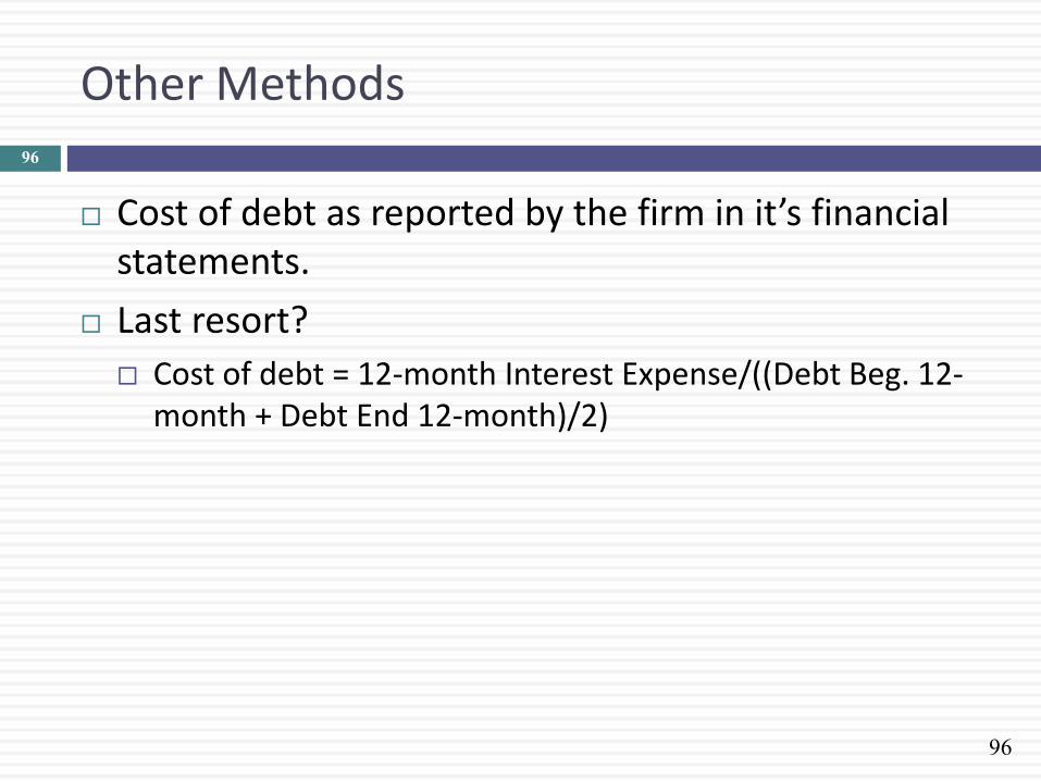
Cost of debt as reported by the firm in it’s financial statements.
Last resort?
Cost of debt = 12-month Interest Expense/((Debt Beg. 12-month + Debt End 12-month)/2)
96
97
Weights for the Cost of Capital Computation
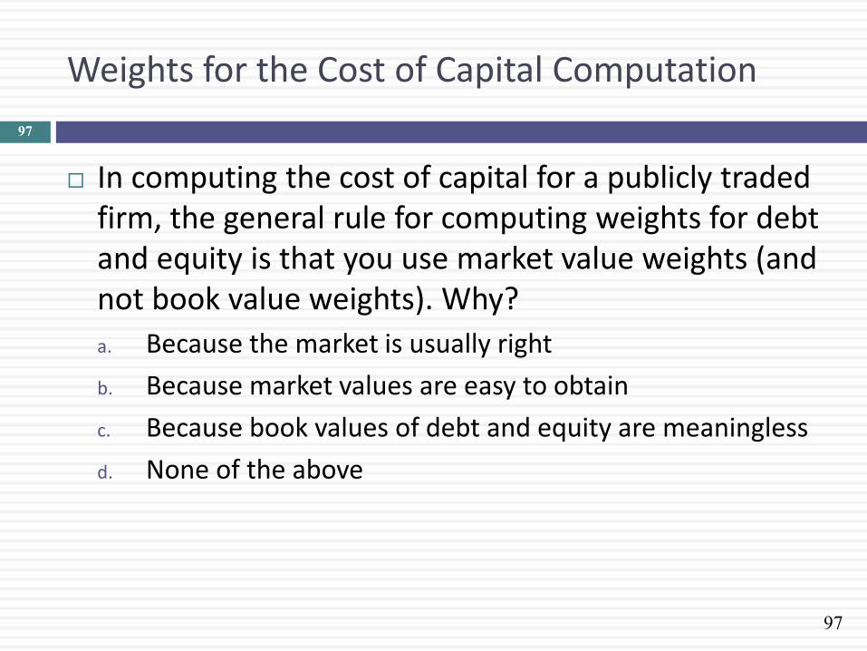
In computing the cost of capital for a publicly traded firm, the general rule for computing weights for debt and equity is that you use market value weights (and not book value weights). Why?
a. Because the market is usually right
b. Because market values are easy to obtain
c. Because book values of debt and equity are meaningless
d. None of the above
97
98
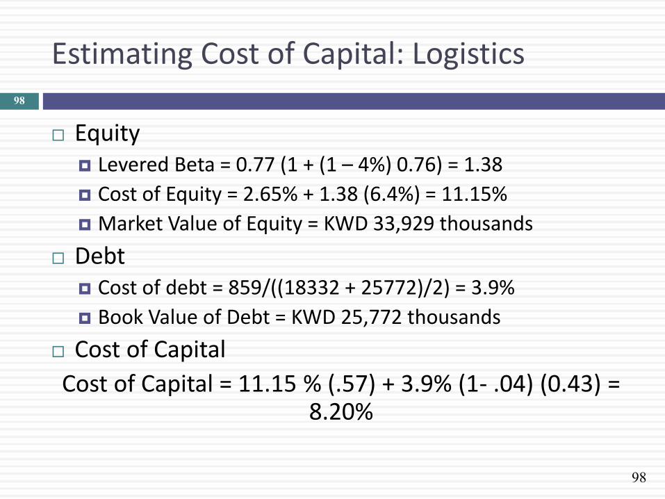
Estimating Cost of Capital: Logistics
Equity Levered Beta = 0.77 (1 + (1 – 4%) 0.76) = 1.38
Cost of Equity = 2.65% + 1.38 (6.4%) = 11.15%
Market Value of Equity = KWD 33,929 thousands
Debt Cost of debt = 859/((18332 + 25772)/2) = 3.9%
Book Value of Debt = KWD 25,772 thousands
Cost of Capital
Cost of Capital = 11.15 % (.57) + 3.9% (1- .04) (0.43) = 8.20%
98
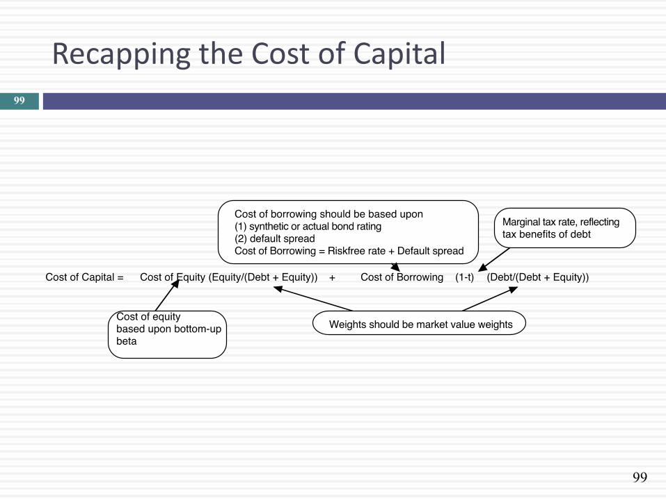
99
Recapping the Cost of Capital 99


