1 Valuation of water quality benefits A spatial hedonic price model Abstract The water framework directive (hereafter WFD) defines quality levels that should be achieved by 2015 in European water bodies. Good status should be reached by implementing sets of measures selected by member states themselves, provided these measures are cost-efficient. In case these costs would appear to be disproportionate, initial quality requirements could be reduced. The issue of dis-proportionality is not clearly defined in the WFD, and one could think of comparing costs and benefits associated to water quality to justify her decision making. The definition of such benefits is not mentioned in the directive and its valuation even less. In this paper, we present values associated to different water quality levels resulting from the estimation of a spatial hedonic price model. To our knowledge, this is the first time the spatial structure of the data is accounted for in the context of the valuation of this environmental good. Our empirical application pertains to a zone managed by a Dutch water board, the Dommel, located in the southern part of the Netherlands. We focus on two water quality indicators: nitrogen concentration and secchi depth. Results are based on the estimation of a spatial error model by the generalised method of moments. Based on our sample characteristics and given a discount rate of 4 percent, an increase in secchi depth by 10 centimetres is associated to a yearly premium of 40 euros per household. Concerning nitrogen concentration, the premium is maximised for a concentration of 4.2 mg/l and amounts to 470 euros per year per household. These results are net of additional benefits related to the proximity to water, which represent a premium of 4.8 percent of the selling price when a house is directly located on the edge of water. These benefits are complemented by distance-based premiums which also depend on the type of water body closest to a dwelling. Key words Hedonic price model, water quality, spatial econometrics
Transcript
1
Valuation of water quality benefits
A spatial hedonic price model
Abstract
The water framework directive (hereafter WFD) defines quality levels that should be achieved by 2015 in
European water bodies. Good status should be reached by implementing sets of measures selected by
member states themselves, provided these measures are cost-efficient. In case these costs would appear to
be disproportionate, initial quality requirements could be reduced. The issue of dis-proportionality is not
clearly defined in the WFD, and one could think of comparing costs and benefits associated to water
quality to justify her decision making. The definition of such benefits is not mentioned in the directive
and its valuation even less. In this paper, we present values associated to different water quality levels
resulting from the estimation of a spatial hedonic price model. To our knowledge, this is the first time the
spatial structure of the data is accounted for in the context of the valuation of this environmental good.
Our empirical application pertains to a zone managed by a Dutch water board, the Dommel, located in the
southern part of the Netherlands. We focus on two water quality indicators: nitrogen concentration and
secchi depth.
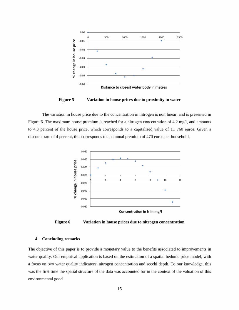
Results are based on the estimation of a spatial error model by the generalised method of
moments. Based on our sample characteristics and given a discount rate of 4 percent, an increase in secchi
depth by 10 centimetres is associated to a yearly premium of 40 euros per household. Concerning
nitrogen concentration, the premium is maximised for a concentration of 4.2 mg/l and amounts to 470
euros per year per household. These results are net of additional benefits related to the proximity to water,
which represent a premium of 4.8 percent of the selling price when a house is directly located on the edge
of water. These benefits are complemented by distance-based premiums which also depend on the type of
water body closest to a dwelling.
Key words
Hedonic price model, water quality, spatial econometrics
2
1. Introduction
The water framework directive (hereafter WFD) defines quality levels that should be achieved by 2015 in
European water bodies. Good status should be reached by implementing sets of measures selected by
member states themselves, provided these measures are cost-efficient. In case these costs would appear to
be disproportionate, initial quality requirements could be reduced, or initial delays given to member states
for the achievement of these requirements could be extended. The issue of dis-proportionality is not
clearly defined in the WFD, and one could think of comparing costs and benefits associated to water
quality to justify her decision making. The definition of such benefits is not mentioned in the directive
and its valuation even less.
Our interest goes to the provision of a monetary value to the benefits associated to the
improvement of water quality. We are interested in covering both use and non-use values. In this paper,
we present values associated to different water quality levels resulting from the estimation of a spatial
hedonic price model. Our empirical application pertains to a zone managed by a Dutch water board, the
Dommel, located in the southern part of the Netherlands. We focus on two water quality indicators:
nitrogen concentration and secchi depth.
This paper is organised as follows. Section 2 exposes the hedonic price methodology and its
spatial extension. Section 3 describes the Dommel region and reports our empirical application together
with preliminary results. The last section concludes.
2. Hedonic valuation of water quality benefits
Water quality benefits are usually estimated by stated preference techniques such as contingent research
frameworks. This means that individuals are directly asked for their willingness-to-pay (hereafter WTP)
for a given improvement in water quality. A main advantage for the researcher is that contextual
information can be given to respondents, such as current quality levels or impacts of quality
improvements. But a major drawback is that respondents can report behaviours that do not correspond to
what they would do in real life situations. This is known in the literature as the hypothetical bias. Several
studies have tried to isolate methodological aspects from other determinants of bias in estimated WTP,
and it appears that individuals have a tendency to overstate their willingness to pay especially when faced
with the valuation of public goods, which can thus be expected in the context of water quality benefits.
List and Gallet (2001) justify such disparity by the lack of experience consumers have to value public
goods as opposed to private ones. Another drawback of this technique is that elicited values are specific to
a given water use, which complicates generalisation of water quality improvement to all water uses.
3
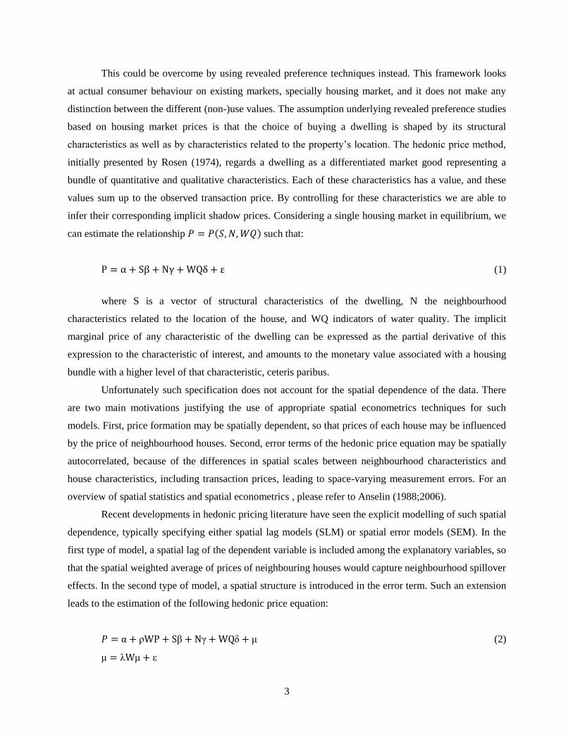
This could be overcome by using revealed preference techniques instead. This framework looks
at actual consumer behaviour on existing markets, specially housing market, and it does not make any
distinction between the different (non-)use values. The assumption underlying revealed preference studies
based on housing market prices is that the choice of buying a dwelling is shaped by its structural
characteristics as well as by characteristics related to the property’s location. The hedonic price method,
initially presented by Rosen (1974), regards a dwelling as a differentiated market good representing a
bundle of quantitative and qualitative characteristics. Each of these characteristics has a value, and these
values sum up to the observed transaction price. By controlling for these characteristics we are able to
infer their corresponding implicit shadow prices. Considering a single housing market in equilibrium, we
can estimate the relationship 𝑃 = 𝑃 𝑆,𝑁,𝑊𝑄 such that:
P = α+ Sβ+ Nγ+WQδ+ ε (1)
where S is a vector of structural characteristics of the dwelling, N the neighbourhood
characteristics related to the location of the house, and WQ indicators of water quality. The implicit
marginal price of any characteristic of the dwelling can be expressed as the partial derivative of this
expression to the characteristic of interest, and amounts to the monetary value associated with a housing
bundle with a higher level of that characteristic, ceteris paribus.
Unfortunately such specification does not account for the spatial dependence of the data. There
are two main motivations justifying the use of appropriate spatial econometrics techniques for such
models. First, price formation may be spatially dependent, so that prices of each house may be influenced
by the price of neighbourhood houses. Second, error terms of the hedonic price equation may be spatially
autocorrelated, because of the differences in spatial scales between neighbourhood characteristics and
house characteristics, including transaction prices, leading to space-varying measurement errors. For an
overview of spatial statistics and spatial econometrics , please refer to Anselin (1988;2006).
Recent developments in hedonic pricing literature have seen the explicit modelling of such spatial
dependence, typically specifying either spatial lag models (SLM) or spatial error models (SEM). In the
first type of model, a spatial lag of the dependent variable is included among the explanatory variables, so
that the spatial weighted average of prices of neighbouring houses would capture neighbourhood spillover
effects. In the second type of model, a spatial structure is introduced in the error term. Such an extension
leads to the estimation of the following hedonic price equation:
𝑃 = α + ρWP+ Sβ+ Nγ+WQδ+ μ (2)
μ = λWμ+ ε
4
with W a spatial weight matrix; λ=0 for an SLM specification and ρ=0 for an SEM specification.
Note that it is common practice to express the hedonic price equation under its semi-log form.
For both types of models, the use of OLS would be inappropriate as it would lead to biased
coefficient estimates of the SLM model because of endogeneity problem and to inefficient coefficient
estimates of the SEM model. Both models can be estimated by maximum likelihood. It is also possible to
apply an instrument variables estimator for SLM and to use the method of moments to estimate SEM.
Specification choice is based on Lagrange multiplier tests (hereafter LM tests) on the restricted model
estimated by OLS where λ=ρ=0, against the SLM or SEM alternative. Robust versions of these tests
(hereafter RLM) account for the fact that these diagnostics have power against the other alternative. These
tests are part of the spatial diagnostic tests.
Hedonic price models have been widely applied in the context of environmental goods valuation,
and spatial specifications are more and more common in recent years: Gawande Jenkins-Smith (2001) on
transportation of nuclear waste; Kim et al. (2003) on air quality; Brasington and Hite (2005) on air, water
and soil pollution; Bin et al. (2008a;Bin et al. 2008b) and Daniel et al. (2007) on floodplain location and
Daniel et al. (2009) for a review; Anselin and Lozano-Gracia (2008) on air quality.
Hedonic price models have also been applied in the context of valuation of improvements in
water quality though to our knowledge not using spatial econometrics. Poor et al. (2007) have reported
hedonic values of ambient water quality measures as suspended solid and dissolved inorganic nitrogen.
Other studies include Epp and Al-Ani (1979), Boyle et al. (1999), Gibbs et al. (2002), Steinnes (1992) or
Leggett and Bockstael (2000).
Finally, findings for the Netherlands are reported in Brouwer et al. (2007). Transaction prices of
houses located in proximity to the water are 2.9 percent higher than average prices for the year 2005. In
terms of quality, a clear visibility of water increases transaction prices by 0.5 percent for each 10cm of
insight gain in the closest water (respectively 0.3 and 0.2 percent for streams and canals).
3. Case study: the Dommel area
NVM, the Dutch Association of Real Estate Brokers and Real Estate Experts, provides data on property
values, reflecting transactions occurring 2005 in the Dommel, together with a comprehensive list of house
characteristics. This data is coupled to neighbourhood characteristics and geographic information on
water bodies. On the one hand, we are willing to capture the utility households have for living nearby
water bodies (sight-seeing, green environment, access to sport activities). These values shall not be
negligible in the region, as the water board the Dommel provides maps and routes for the following
5
activities: bathing, canoeing, rowing, sailing, but also biking, trekking and site seeing. On the other hand,
we want to capture their preference for clean water. To do so, we create variables reflecting proximity to
water for each house in our data set, and associate each dwelling to water quality indicators.
First, we determine the distance between each dwelling and the closest water segment, per type of
water body. Water bodies can be rivers, canals, lakes or city water. We also compute the distance between
each dwelling and the closest official swimming location. In the Dommel, there are currently 23 bathing
locations, which are advertised by the Province Brabant as official – thus safe – bathing locations, and are
subject to regular monitoring for checking the presence of bacteria and algae. The results of these
screenings are publicly available. We complete this set of distance variables with an indicator of water
richness in the close neighbourhood of each dwelling. This indicator is defined as the percentage of
ground surface covered by water in a one square kilometre area around the dwelling, and can take values
lying between 0 and 100.
Then for each house, we associate two water quality indicators, the concentration in nitrogen in
mg/l and secchi depth in decimetres, which is a measure of the turbidity or cloudiness of water. These two
measures are reported by the national emission register1 for a certain number of monitoring stations. We
consider yearly average in 2005 of these test results. We then link this monitoring data to the water body
it refers to, and we associate for each house the monitoring data of the closest water body that happens to
have such data.
We have information for 5358 transactions in a region comprising the main cities Boxtel, Tilburg
and Eindhovein. Figure 1 shows the distribution of transactions in this region. Each dot represents a house
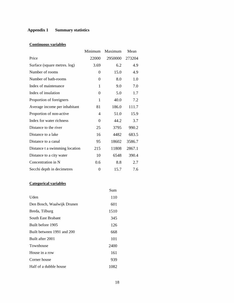
sale. Summary statistics for the whole dataset are presented in Appendix 1.
Table 1 presents summary statistics for water related variables. It appears that water is broadly
present in the region, where all houses are located on average within less than 400 meters to city waters.
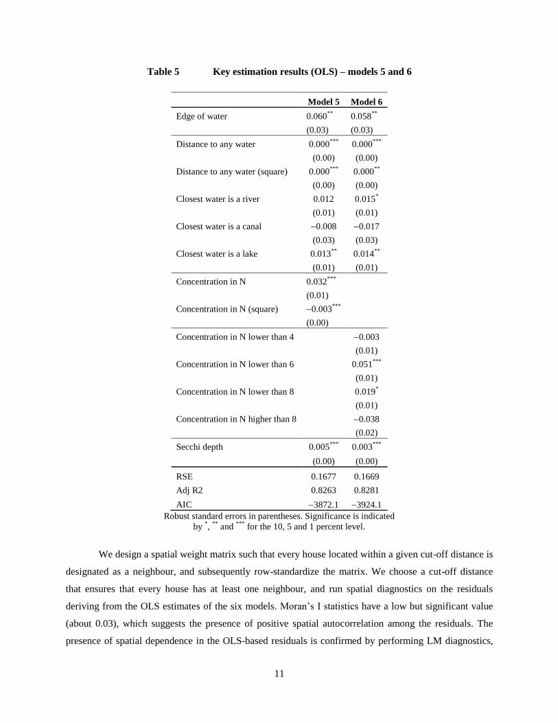
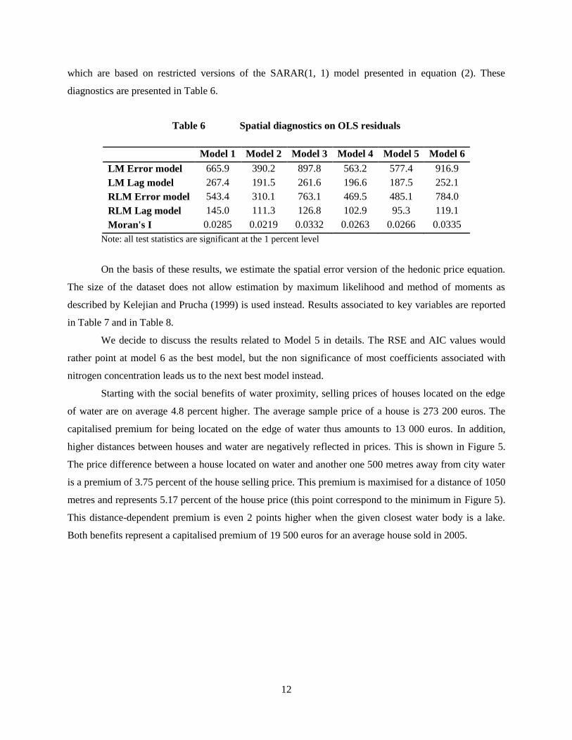
Table 1 Summary statistics – water variables (all distances in metres)