Value Added What??...Horizontal versus Vertical Expansion in Iowa Production Agriculture Josh D. Roe Department of Economics Iowa State University Selected Paper at American Agricultural Economics Association Annual Meeting, July 24-27, 2005, Providence, RI Copyright 2005 by Josh D. Roe. All rights reserved. Readers may make verbatim copies of this document for non-commercial purposes by any means, provided this copyright notice appears on all such copies.
Transcript
Value Added What??...Horizontal versus Vertical Expansion in Iowa Production Agriculture
Josh D. Roe Department of Economics
Iowa State University
Selected Paper at American Agricultural Economics Association Annual Meeting,
July 24-27, 2005, Providence, RI
Copyright 2005 by Josh D. Roe. All rights reserved. Readers may make verbatim copies of this document for non-commercial purposes by any means, provided this copyright notice appears on
all such copies.
ii ABSTRACT
Farm investment in value-added agricultural firms continues to grow in the United States.
Using farm-level, asset allocation models, value added investments were found to be
advantageous for farms with below average earnings or older operators. Farms with superior
financial performance benefited from a portfolio allocation that favored farm expansion.
1 Introduction
Investment in farmer-owned, value-added businesses has skyrocketed since the early
1990s. This shift in farmers’ investment preferences has the potential to transform many rural
landscapes from endless fields to a combination of fields, processing facilities, and additional
animal confinement units. Historically, farmers have added value to their crops through on-farm
livestock production. More recently, farmers have invested in manufacturing facilities to produce
bio-fuels, egg proteins, and other products.
Because increases in value-added agricultural manufacturing in rural areas can stimulate
rural economies, local and national lawmakers are interested in stimulating growth in this area.
As of May 2001, all 50 states had at least one program to assist value-added agricultural
businesses. In the 1998-99 fiscal year, states around the nation budgeted more than $280 million
dollars for value-added agriculture programs (Kilkenny 2001).
Numerous theories have attempted to explain shifts in farmer investment preferences,
growth in farmer-owned businesses, and willingness of the government to subsidize value-added
agriculture. Two reasons suggested are the overall change in farm structure and the need for rural
development.
As farms have grown over the past century, they have also increased in complexity.
Today, farmers are also managers, marketers, and operators. As farm size has increased, the
number of farmers has dramatically decreased. This trend toward fewer, larger farms has resulted
in more competitive, qualified farmers, both locally and internationally.
Along with the growth in farm complexity is worldwide pressure on the United States to
reduce direct and loan deficiency payments to farmers. While this limits farm income from
subsidies, with these gradual declines in direct payments comes more flexibility in crop and
2 livestock production decisions. As a result, producers may be looking for alternative ways to
enhance income in the event that direct farm subsidies are terminated.
The increased complexity, farm size, competition, and government payment limitations
have forced farmers to develop new production and marketing opportunities in order to enhance
farm incomes. An overall and popular attitude towards becoming more competitive in the
worldwide marketplace is to add value to basic commodities by processing them into
differentiated food products or finding non food uses.
New farmer-owned businesses can potentially increase rural incomes by providing new
jobs, hence stimulating the local economy and widening the tax base. Many new farmer-owned
businesses are locating near rural areas because of the proximity of primary inputs.
Traditionally, growth in farm size, or horizontal expansion, was seen as the only option
for producers to combat highly volatile farm incomes in the face of real declines in output prices
along with real increases in input prices. In the case of fa rm expansion, average costs decline
over certain levels of production due to economies of scale. There is little research evidence that
suggests that average costs will increase rapidly at increased levels of output in US agriculture
(Cooke 1996). However, technical barriers such as access to additional land and capital can limit
farm expansion at some point.
A variable relevant to farmers in addition to increasing or decreasing production costs is
how farm expansion affects the variability of farm income. As a farm expands, the level of farm
income is expected to increase. However, the level of variability of farm income may not
decrease, but increase due to larger investments in a similar, if not identical, commodity.
An alternative to horizontal expansion is to vertically expand through investments such as
a farmer-owned, value-added business. This may allow producers to capture or create more value
3 from products originating from farm commodities. This is in direct contrast to a situation in
which the producer only owned the commodity in its basic form, and then sold it to another firm,
which transformed it into another state while sharing no ownership with the producer.
The two questions that this research will attempt to answer are (1) whether vertical or
horizontal expansion is more profitable for agricultural producers and (2) what attributes of an
individual farm make it more efficient for them to vertically or horizontally expand. In
answering this question, the possible advantages and disadvantages to adding value-added
investments to a portfolio of farm assets will be explored. Additionally, the attributes that make
non-farm assets attractive to farmers will be identified.
Conceptual Framework
The choice of vertical or horizontal expansion by individual farmers is an empirical
question. Therefore, empirical results are needed in order to determine whether vertical or
horizontal expansion is more efficient for Iowa producers. We will discover results through
portfolio analysis.
To begin, we assume that a producer is considering whether or not to expand his/her
current farm operation or to invest in some form of vertical expansion, including value-added
agricultural manufacturing and/or stock market investments. Taking into account his attitude
toward these risks, the producer will optimize his portfolio holdings in farm and non-farm asset
expansion based on expected risks and returns. The producer is assumed to optimize his holdings
such that his portfolio lies on the lend/borrow line between the risk-free rate of return and the
point of tangency with the Markowitz’s E-V frontier as illustrated in Figure 1.
4 There are several quantitative asset allocation models that will optimize an investor’s
portfolio. However, since we had no access to each investor’s risk aversion coefficient, this
research will utilize Sharpe ratio maximization.
William Sharpe, who developed the Sharpe ratio in 1966, described it with the coined
term “reward-to-variability.” Along the lines with portfolio allocation, if a portfolio is balanced
such that the Sharpe ratio is maximized, that portfolio is said to be on the E-V frontier;
mathematically:
( )( )
pii
pi
E R rfS
E Var−
=
Where:
E[Rpi]=Expected return of portfolio i.
E[Varpi]=Expected variance of portfolio i.
rf=Risk-free rate of return
The Sharpe ratio is equal to the slope of the lend/borrow line. Therefore, maximizing the
Sharpe ratio will maximize the lend/borrow line’s slope, indicating that the portfolio has the
greatest expected return given the risk-free rate of return.
Investing in Farm Expansion
Farmers have historically relied on horizontal growth or expansion as a strategy to
improve their financial positions. A consequence of horizontal growth is increased farm size, the
substitution of capital for labor, and an increased risk exposure due to specialization and
relatively constant average costs.
However, due to physical constraints such as land availability in close proximity to the
existing farm operation, farm expansion may be limited. Producers may also lack the available
5 capital to further expand their farms if there is no additional land or facilities available for lease
and have to purchase a sizeable tract of land or build additional livestock facilities.
Studies conducted on farm expansion found that actual cases of rising average costs with
additional output in American agr iculture are very rare (Cooke 1996). Work evaluating the cost
advantages of large scale farms concluded that farms with more than 2,500 acres of corn could
purchase production inputs for as much as 20% less than smaller corn farms (Krause 1971). It
has also been concluded that large farms are more likely to adopt and gain the benefits of
increased technologies than smaller farms (Stanton 1987).
Investing in Value-Added Agriculture
Over the past decade, farmers have been encouraged to consider investments in value-
added agriculture as an alternative to farm expansion and a way to avoid the economies-of-scale
treadmill that continually requires expansion to stay competitive. By investing in value-added
agriculture, firms can capture value downstream from their production process. In 2004,
producers received less than 20% of the value of gross US food expenditures, with the balance
going to the value adding sector (USDA).
Value-added agricultural investments may also improve the diversification of the farm’s
portfolio. For example, suppose a farmer whose major output is corn owns shares in a business
whose major input is corn. Holding yield constant, in years where corn prices are relatively low,
farm returns will be also be relatively low. However, during these low price periods, the return to
the value-added business will be relatively high.
Value-added agricultural investments may also be desirable because farmers are better
informed than non-farm investors. A farmer is also more likely to know more about an
investment involving his commodity (i.e. corn processing company) than an investment that has
6 little or nothing to do with his commodity (i.e. aerospace engineering firm). Hence investments
in value-added agriculture may be more enticing to producers due to their more in-depth
knowledge of the subject.
As stated earlier, a majority of new value-added agriculture businesses are locating in
rural areas. If a new value-added agricultural business has considered locating in close proximity
to a producer’s operation, he may be more willing to invest in the business. His support can stem
from an expectation that the new business may create local jobs and increase the local tax base or
from the hope that the new business will provide an additional marketing channel for his
commodity. The producer may also be able to monitor the business activity directly or through
social networks.
However, these apparent benefits from investment in value-added agriculture also come
with risks. These risks are especially likely if the investment requires significant capital outlays
to purchase processing facilities and to hire management and marketing staff.
Startup costs for a value-added business may be large, requiring both significant capital
investments as well as substantial commitments of the commodity from the investors.
Consequently, debt financing would need to be obtained from bonds and/or from private
financial institutions. If this additional financing is required, investors will likely hold a residual
claim to early profits incurred by the business and may lose their entire investment if the entity
fails.
Research analyzing value-added agriculture investments by hog and cattle producers has
been recently conducted. These studies concluded that a portfolio consisting of value-added
investments and farm assets provides better returns and lower risk than a portfolio consisting of
farm assets alone (Detre 2002), (Jones 1999).
7 Investing in Stock Indexes
Investments in agricultural firms not closely tied with farm returns or those that have no apparent
correlation with farm returns are also readily available to producers. These investments include
investment in a stock market index or in a portfolio of food and agribusiness stocks. These
investments can be viewed as alternate routes of vertical expansion for the farm since the
structure of these investments are substantially different from those of value-added agricultural
manufacturing.
Producers may benefit from investing in a mutual fund such as the type that contains the
same stocks as those measured in the S&P 500. These indexes will increase the value of a
portfolio over time due to the long-term upward movements in the financial markets. Investment
in an index also provides portfolio diversification because its movement is contingent on many
more factors than those affecting agricultural markets.
Another benefit to this investment is its liquidity. A producer can buy and sell mutual
funds in these indexes at any time and in varying amounts. In contrast, an investment in a single,
value-added agriculture business may be a fixed amount, require delivery of a significant amount
of corn or soybeans, and may not be as liquid as a widely- traded mutual fund.
Since these indexes capture the entire market, the investor bears virtually no unsystematic
risk with the addition of the asset. However, even though this method should increase equity
over a long horizon, it provides little short and intermediate term assurance because farm and
financial markets may not be correlated. Several instances of this lack of correlation between
farm and financial markets occurred in the 1920s. The farm market was in collapse following
World War I, while the financial market was experiencing the “Roaring 20s” (negative). The
farm crisis in the 1980’s coincided with rampant unemployment and inflation (positive). Also,
8 the technological boom in the mid 1990s in the stock market coincided with the Asian crisis in
the agricultural sector (negative). Therefore, investing in a market portfolio may not completely
mitigate production risks encountered by a producer.
Studies show that when producers invest in stock indexes, it is a viable investment.
Research evaluating stock index investment in addition to farm assets concluded that in times of
highly variable farm incomes, investment in stock indexes can reduce expected risk and increase
return (Serra 2003).
Investing in Food Processing and Agribusiness Stocks
Investing in food processing companies and agribusiness stocks that are involved in the
processing and marketing of agricultural commodities presents a similar opportunity to capture
downstream profits than investing in a value-added business.
The main difference between this investment and investment in a local value-added
business is mainly that the company will be less likely to be in close proximity to the farm
enterprise and the producer will have even less management power. This is because to many
food and agribusiness stocks, the expense of the raw agricultural commodity is significantly less
than for a smaller scale farmer-owned, value-added agriculture business. In general, commodity
inputs are a small part of their costs. Since a majority of these firms’ costs are labor and
management, they will likely choose to locate near specialized labor pools in urban areas
(Kilkenny 2001).
However, these differences bring possible benefits. The company is likely to be located
in an optimal location, which may give it access to a better skilled and more specialized labor
and management pool than a business located in a rural area. Investment in agribusiness
companies has the same liquidity as stock indexes. However, the investor may be prone to both
9 unsystematic and systematic risks and returns. If their returns are relatively less correlated with
farm returns, diversification benefits may also be lost. Studies evaluating the addition of food
and agribusiness stocks to a farm asset portfolio concluded that they capture additional benefits
beyond diversifying with stock indexes (Featherstone 2002).
Model Specification
The asset allocation problem is solved by maximizing the expected Sharpe ratio for each
farm in the sample by varying the portfolio weights of each asset. Using time series data, the
basic Sharpe Ratio is specified as:
1 1
2
1 1
5
1
( * )
max
( * * )
.
. 1
0 1
n k
j ji j
f
n k
j j j ji j
jj
j
w rr
nS
w r w r
ns t
w
w
= =
= =
=
−=
−
=
≤ ≤
∑∑
∑∑
∑
Where:
n=Number of periods
k=Number of assets
wj=Weight of asset j,
rj=Return of asset j in period i
jr =Expected mean return of asset j
rf=Risk-free rate of return.
10 In a one period, or static approach, the Sharpe ratio does not account for correlation
among the investment alternatives. When the multi-period form of the Sharpe ratio is used to
estimate optimal portfolio weights, the formula for portfolio variance incorporates covariance
among assets. Once the above expression is maximized subject to its constraints, the portfolio is
considered to be on the efficient frontier. Previous studies have used this multi-period form of
portfolio optimization in evaluating asset choice models for agricultural producers (Detre 2002).
The Solver add- in to Microsoft Excel was used to maximize the Sharpe ratio to acquire a
unique portfolio for each farm. The risk-free rate of return was assumed to be 3%, and is
consistent with an average rate of return from a relatively low risk asset in today’s market.
Detre (2002) used the Sharpe ratio in this form to optimize a portfolio for agr icultural
producers. However, in that particular study, farm returns were averaged across the state so a
single average portfolio was optimized. However, individual portfolio results can provide more
detailed results and when averaging returns across the state across multiple years, the true in
farm-level returns can be significantly underestimated.
Portfolio Result Interpretations
Because one investment is mutually exclusive to each agent (their farm returns), their
optimal portfolios will be unique. In other words, each agent has a uniquely shaped efficient
frontier because of unique portfolio investment opportunities. Figure 2 illustrates different E-V
frontiers and tangency points for two (hypothetical) individuals with access to the same risk-free
rate of return As illustrated, individual b has access to higher rates of return given a leve l of risk
due to farm returns larger than a, or a stronger negative covariance among potential assets.
In effect, the fact that each producer has a unique investment alternative is parallel to a
custom product given to an investor due to each farms’ unique returns. Because of this, the
11 argument that the capital asset pricing model does not account for individual characteristics is
ignored because each individual is given a mutually exclusive investment alternative in the form
of his own farm business returns (Featherstone 2002).
Nonetheless, the optimized portfolio weights only reflect the producer’s optimal risk and
return tradeoff given the risk-free or loan rate. Individual demographics and farm characteristics
play little or no role in the optimization outside of the observed farm returns because the
portfolios were optimized using only information about farm and asset alternative returns. In
reality, each producer’s optimized Sharpe Ratio is unique due to economic and demographic
characteristics of the individual. This is because these attributes may directly affect the farm’s
return to expansion, which affects the rates of return that a producer can access.
Therefore, farms that have similar investment patterns may or may not be similar in their
characteristics. To determine this, groups of farmers with similar portfolio weights need to be
identified. This allows the researcher to determine if they are, in fact, similar and if their
individual characteristics affect their portfolio weights. K-Means Clustering was utilized in order
to determine clusters of farms that are similar with respect to their investment weights. For a
rigorous derivation of K-Means Clustering, see Das (2003).
Cluster analysis will determine which farms are similar based on their portfolio weights.
It is hypothesized that each cluster’s efficient frontier will have a similar shape because of
similarities in their optimal risk and return tradeoff. The E-V frontier within clusters will only
vary by the variability of the farm returns and the covariance among asset alternatives.
If individual farm characteristics and demographic variables can be used to predict which
cluster a farm is in, it can be determined if individual farm characteristics affect their optimal
investment patterns. This will answer the question of what characteristics of a farm make it more
12 profitable to invest in vertical or horizontal expansion. Multinomial logit modeling will be used
to link a farm’s characteristics to their optimal investment patterns.
Estimation of Asset Returns
Data on actual Iowa farm characteristics and performance were obtained from the Iowa
Farm Business Association’s annual individual farm records (Iowa Farm Business Association).
Electronic records of the data were available from 1993-2003. A balanced panel of observations
for all years was constructed. The balanced panel dataset contains 191 unique farms that
represent a good sample of commercial operations across Iowa.
Table 1 presents average 1993, 1998, and 2003 values of selected financial and
demographic characteristics of farms included in the dataset. The definitions of ratios used are
presented in Appendix A. Consistent with state and national averages for farms, the operator’s
age, farm size, crop yields, and non-farm income increase steadily throughout the time period.
Interest expense as a percentage of total farm revenues decreased over the time period, likely due
to decreasing interest rates.
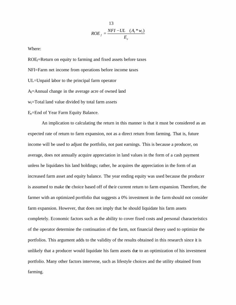
The rate of return for each farm throughout the time period was calculated as the rate of
return on farm equity plus gains in capital asset values. Accounting for gains in capital asset
values allows the rate of return to farming to be compared directly to rates of return on stocks
and business investments. For example, in calculating the rates of return on a stock investment
over the course of a year, both the capital appreciation of the stock’s value and the amount of
dividends earned over the time period are included. Therefore, in calculating the return to
farming, both the increase in capital assets (stock value) and net farm income (dividends) are
included to make these rates of return comparable. The rate of return on farming plus gains in
capital assets for each year was calculated using the following equation.
13
( * )l lf
e
NFI UL A wROE
E− +
=
Where:
ROEf=Return on equity to farming and fixed assets before taxes
NFI=Farm net income from operations before income taxes
UL=Unpaid labor to the principal farm operator
Al=Annual change in the average acre of owned land
wi=Total land value divided by total farm assets
Ee=End of Year Farm Equity Balance.
An implication to calculating the return in this manner is that it must be considered as an
expected rate of return to farm expansion, not as a direct return from farming. That is, future
income will be used to adjust the portfolio, not past earnings. This is because a producer, on
average, does not annually acquire appreciation in land values in the form of a cash payment
unless he liquidates his land holdings; rather, he acquires the appreciation in the form of an
increased farm asset and equity balance. The year ending equity was used because the producer
is assumed to make the choice based off of their current return to farm expansion. Therefore, the
farmer with an optimized portfolio that suggests a 0% investment in the farm should not consider
farm expansion. However, that does not imply that he should liquidate his farm assets
completely. Economic factors such as the ability to cover fixed costs and personal characteristics
of the operator determine the continuation of the farm, not financial theory used to optimize the
portfolios. This argument adds to the validity of the results obtained in this research since it is
unlikely that a producer would liquidate his farm assets due to an optimization of his investment
portfolio. Many other factors intervene, such as lifestyle choices and the utility obtained from
farming.
14 Because of their ease of investment and worldwide popularity, two different stock
investments were included as asset alternatives: Investment in the S&P 500 market index and a
mutual fund consisting entirely of food and agribusiness stocks; the Fidelity Food mutual fund.
Historical data on their prices and dividends were downloaded from Yahoo Finance for 1993-
2003.
Because of their popularity in Iowa, investments in ethanol and egg production were
included as alternatives to farm expansion.
Historical returns to ethanol production were estimated using a spreadsheet that
calculated return on equity for a representative ethanol plant in the Midwest (Tiffany 2004).
Underlying assumptions are that the ethanol plant has a maximum production capacity of 60
million gallons per year; one bushel of corn yields 2.7 gallons of ethanol and 17 pounds of
distillers dried grains with solubles (DDGS). The plant also uses 0.165 million British thermal
units (mmBTU) of natural gas, roughly 2 gallons of water, and 1.04 Kwh of electricity to process
one bushel of corn (Paulson). The short-term interest rate was set at 6% and no tax subsidies or
value-added payments were assumed. The return on equity of the plant was calculated with
average annual corn, ethanol, and DDGS prices for 1993-2003.
Data on returns for egg production were calculated using USDA/ERS and Iowa State
University Extension estimates for costs of production and prices received by farmers for one-
dozen eggs for the time period 1993-2003 (Lawrence 2003) (USDA/ERS 2004). The net returns
per dozen were calcula ted to derive a rate of return on a one dollar investment in an egg
production facility. The returns are estimated for a 110,000 hen facility with building,
equipment, and land costs of $700,000; layers initially cost $2 per bird and follow a 90 week
lay/molt/lay cycle and are disposed of at no value; 1,650 man hours of labor are required
15 annually at the average annual wage rate for farmer workers; and 200,000 kwh of electricity are
required annually at the average annual commercial rate (Lawrence 2003). Tables 2 and 3
present the average returns and the correlations among the four asset alternatives by year.
Over the time period, the layer facility is the investment with the lowest measures of risk
and return. The steady returns can be attributed from a steady growth in the demand for eggs
over the time period. However the real increase in the price of eggs and energy limited the
returns to egg production. The Fidelity Food mutual fund yields the highest expected return
while the S&P 500 is expected to vary the greatest. These investments performed well at the
beginning of the time period but decreased due to the drop in the stock market in the late 1990s.
The ethanol plant investment is the riskier of the two value-added stocks, but its risk appears to
be less than that of the Fidelity mutual fund. The ethanol plant’s returns increased as the time
period progressed due to increases in the price of DDGS and ethanol, while the price of corn
decreased overall.
Egg, ethanol, and stock investments are positively correlated throughout the time period.
However, the correlation is weaker for ethanol. Egg and ethanol production returns appear to be
uncorrelated. This may occur because of large differences in the market for ethanol and eggs. As
one might expect, the correlation between the two stock investments is positive.
Operator Demographic Hypotheses
Operator Age
As a farm operator’s age increases into their senior years, their investment preferences
can shift two ways. If the operator views his increasing age as a signal to be more conservative
with his money, he will choose to invest excess farm equity into an investment that provides a
viable return at very low risk levels. At this point in their investment experience, he will know
16 the risks and returns associated with the expansion of their operation with fair certainty. If he
views his farm’s return as stable and adequate, he will choose farm expansion. However, if he is
unsatisfied with the risks and returns of his operation, he may choose to invest in an alternative,
such as a value-added agricultural business if he believes the investment consequences will be
positive. Another factor that might encourage non-farm investments is if they view themselves as
unable to take on additional operational and management labor to manage a bigger farm, because
non-farm investments will require significantly less labor. Older producers may also have more
liquid assets to disperse into a non-farm business compared to a producer who is relatively
younger.
In this modeling framework, we only have information on a farmer’s age and farm
returns, not information on how a farmer views his farm returns and the returns to a value-added
agricultural business. Thus we must explore the correlation between age and investment choices
by looking at the correlation between farm productivity and the age of the operator. Previous
studies linking the age of an operator to farm productivity concluded that farm productivity
increases with operator age until the operator is roughly in his mid- to late- 40s, then farm
productivity decreases while the operator continues to age. This decrease in productivity occurs
because of his declining physical labor productivity and unwillingness to adopt new, labor saving
technologies (Tauer 2000). Other studies have stated that the rate at which an operator expands
his operation increases into his mid-thirties, then declines at a non- linear rate with age until no
further farm expansion occurs (Weiss 1999). If the results of this research align with previous
studies, then the negative relationship between operator age and farm returns will shift the
optimal investment mix to a portfolio of asset alternatives (besides farm expansion), for clusters
with a higher mean age, ceteris paribus.
17 Non Farm Income Levels
A producer’s level of non-farm income can have a significant effect on his investment
choices. A producer with a larger non-farm income than another will have more off farm time
commitments; whether the commitments are a full time job outside of the farm or actively
managing a stock portfolio. Hence, clusters with a relatively higher non-farm income should be
more prone to invest in non-farm assets because they are unable to provide more farm
management labor.
Farm Leverage
A producer with a significant amount of farm debt can be looked upon as a risk tolerant
individual or one with poor financial management skills. In either case, it is hypothesized that
significant farm debt levels should trigger off farm investments. In the case of poor financial
management skills, the producer might not be willing to expand an already inefficient operation
or may not have access to adequate credit in order to expand, hence encouraging non-farm
investments. In the case of a risk tolerant operator, outside investment may be viewed as an
opportunity for additional income. The level of uncertainty associated with non-farm investments
will not heavily weigh into their decision. Therefore, clusters with high debt levels should also
choose vertical expansion.
Farm Profitability
A producer with a relatively profitable and productive farm operation will mainly choose
to expand the farm up to his limit of management labor available and/or the availability of
additional land and capital. However, if he has reached these limits or can see benefits in non-
farm investments, he may choose non-farm investments. Due to their above average and stable
farm returns, he will be more likely to invest in investments that have the highest expected
18 returns, even if they bring on more uncertainty, because of their current low levels of risk.
Therefore, if there is a strong negative correlation to farm returns to vertical investments within
certain clusters, they will optimally choose vertical expansion.
Farm Type
The primary commodities produced by a farm will have a significant effect on a
producer’s investment decisions due to their different marketing channels. For instance, a
producer who feeds a majority of his crops to his own livestock has less need for an additional
marketing channel than a producer who sells a majority of his crops on the open market.
Producers who sell a majority of their crops on the open market are not currently adding any
value to their commodities, thus an outside investment into an entity that adds value to their
commodity will be enticing to them because it provides an additional marketing channel. Also, if
the negative correlation between farm returns and value-added businesses that was discussed
previously occurs in most years, the outside investment will lower their portfolio’s risk.
The results of the multinomial logit model will test the above hypotheses and quantify
their effects. This will allow us to evaluate one of the main objectives of this research: What
factors will affect the efficiency of a farm to expand horizontally or vertically?
Results and Interpretation
For the Sharpe ratio maximization, the average portfolio is balanced mainly between
farm expansion and egg production. Due to their relatively large expected risk when compared to
farm expansion, ethanol, and egg production, stock investments do not play a role in the
portfolio.
Figures 3a-e illustrate the distributions of farm expansion and asset alternative weights
yielded by Sharpe ratio maximization.
19 As Figure 3a illustrates, producers would optimally choose a wide variety of portfolio
weights for farm expansion. The optimal weights on farm expansion vary wider than any other
asset because the returns to farm expansion are unique for all 191 observations, whereas returns
available from the other four asset alternatives are the same. About 40% of producers would
optimally place little or none of their portfolio in the ethanol plant with about 30% placing 10-
20% and 20-30%. Because of its low risk, as figure 3c illustrates, producers would optimally
choose to balance their portfolios with a wide range of egg production. Its relatively low risk and
high return give producers an opportunity to lower their expected portfolio variance.
Producers, in general as figures 3d-e illustrate, would optimally limit stock market
investments due to their high risk relative to the other assets. However, it is worth noting that a
few producers would optimally choose to invest in as much as 40% S&P 500 and 25% Fidelity
Food. Further investigation into these farms reveals that their expected return from farm
expansion is much greater than average with relatively small fluctuations. These producers could
optimally take on the high risk stock investments for a greater expected return because they have
a relative low amount of risk in farm expansion.
Cluster Analysis
As previously discussed, the optimal portfolio weights estimated by the Sharpe ratio
model only reflect the estimate of risk, return, and covariance among the five assets. These
differences, namely the shape of their individual E-V frontiers, are due to each farm’s unique
characteristics. In order to quantify these characteristics, we need to determine which farms are
similar to one another with respect to their portfolio weights.
Table 4 shows the summary statistics for different values of k clusters that were
considered. As k increases, the maximum Euclidean distance within the clusters decreases, which
20 indicates that farms inside each cluster are more alike. However, notice that when the number of
clusters allowed increases above five, the number of farms in each cluster falls to as low as one.
From a statistical and economic view, a cluster containing one observation is not significant.
Also, in general, as the number of clusters increase, the distance between the nearest clusters
decrease, leading one to believe that the clusters are not that different. The F-Statistic tests the
hypotheses that the difference between each cluster and its closest counterpart is equal to zero.
The F-Statistic peaks at five clusters. Since the F-Statistic peaks at five clusters and reducing k to
four makes little difference in the number of farms per clusters, we used the five-cluster model in
our further analysis.
Table 5 presents summary statistics for each cluster for 2003, Appendix A contains
financial ratio definitions. Figure 4 illustrates the distribution of average portfolio weights for
each cluster.
The farm characteristics of each cluster given in Table 5 and their respective portfolio
weights in each asset revealed key differences among clusters. Cluster 4 has an average of 88%
of its optimal portfolio in farm expansion, the largest percent of any cluster. Cluster 4 also has
the largest average corn and soybean yields; the lowest debt to asset ratio; the highest net farm
income ratio, return on assets, and profit margin; while having the lowest interest expense ratio.
In contrast, Cluster 1 has an average of 8% of its optimal portfolio in farm expansion, the
smallest percent of any cluster. Cluster 1 has the lowest average net farm income, return to
management, and profit margin while having the highest interest expense ratio. Cluster 1 also has
the highest non-farm income and the largest average farm size, indicating that non-farm
employment may hinder additional farm expansion and due to their relatively larger size, might
have reached a limit to farm expansion.
21 Cluster 2 has the fewest farms – only five. As Figure 4 indicates, the primary reason they
are separately partitioned is that it would be optimal for them to hold significant investments in
the two stock assets compared to the other four clusters. From a farm characteristic aspect they
are the youngest operators and hold 57% of their portfolio in farm expansion. Nonetheless, they
earn the highest net fa rm income, return to management, and return on equity, while having the
lowest operating expense ratio. Their relatively stable farm return on equity may allow them to
take on the higher risk assets to increase expected portfolio return. They have the highest
expected portfolio return, for a lower level of risk.
In the figure 5, each farm’s average portfolio return less the risk free rate is plotted
against portfolio standard deviation. A trend line is estimated assuming a common intercept of
zero. This allows direct comparison of the slopes of each cluster’s trend line. As the differing
slopes of the cluster trend lines indicate, each cluster has a unique risk and return tradeoff. For
example, the slope of the trend line for Cluster 4 is the steepest, indicating that these producers
expected portfolio return is higher while taking on less risk, compared to the other four clusters,
which have smaller slopes for their trend lines. Cluster 2 has a slope similar to that of Cluster 4,
but with only five producers in Cluster 2, the validity of its true slope is questionable. Clusters
1and 5 have the smallest trend line slopes, indicating that their level of return for a given amount
of risk is inferior to the other three clusters. This indicates that each cluster’s E-V frontier has
similar slopes while the E-V slopes between clusters are significantly different.
These results are in line with previous hypotheses stating that since farm expansion is the
only firm-specific investment available to the producers, the slopes of each E-V frontier will
differ. This is also inline with the previous hypothesis stating that those farms with the greatest
22 returns to farm expansion given a level of risk will have the steepest E-V frontier slopes. Clusters
1and 2 have the highest mean farm returns, and in turn, they have the steepest E-V frontiers.
Multinomial Logit Results
A multinomial logit model was estimated using the cluster number assigned to each farm
as the dependent variable. The explanatory variables used include average operator’s age, grain
sales ratio, net farm income ratio, return on equity, debt to asset ratio, interest expense,
government payments ratio, and non-farm income. Tables 6 and 7 contain the parameter
estimates for each B and the marginal effects of the logit model.
Overall, the model does an adequate job of predicting a farm’s cluster based on the
explanatory variables, using the pseudo R2 and absolute value of the log likelihood function as
measures. All explanatory variables are statistically different from zero across at least one
cluster. Table 4.6 illustrates the parameter estimates of each characteristic relative to Cluster1.
The marginal effects of each explanatory variable in each cluster are displayed in Table 7.
For the most part, all of the explanatory variables have the expected signs and they
provide some very intuitive economic points. For example, Clusters 1 and 5 invest the least in
farm expansion, but they invest heavily in the value-added agricultural businesses. The marginal
effects for the grain sales ratio are positive for these two clusters and negative for the other three.
This states that as a farmer relies more on the open market for the sale of his crops, he is more
likely to invest in value-added agriculture. This meets the previous hypotheses that value-added
investments will be attractive to cash grain farmers due to the addition of another marketing
channel and the negative correlation between the value-added agricultural businesses and farm
returns. As Table 8 illustrates, the correlation between farming and ethanol returns throughout
1993-2003 was -0.249, which can be viewed as a negative correlation. The correlation between
23 farming and egg production was 0.063, which is positive, but small enough to conclude the
correlation is insignificant.
The marginal effect on the net farm income ratio is negative for clusters 1and 5 but
positive for clusters 2, 3, and 4. As Table 5 illustrates, the farms in Clusters 2-4 are more
profitable than Clusters 1 and 5, so Clusters 2-4 place significant holdings in farm expansion. So,
as the net farm income ratio rises, the farm is more profitable and productive, hence the farm is
more likely to be in a cluster that invests heavily into farm expansion.
The marginal effect on the operator’s age is also negative for Clusters 1 and 5 but
positive for Clusters 2-4. As far as this research is concerned, as a farmer gets older (Clusters 1
and 5 have the highest average operator age), he is more likely to invest in non-farm assets and
less likely to expand his farming operation. This is in line with previous research that shows that
as an operator’s age increases, farm productivity declines. Clusters 1 and 5 have the lowest net
farm income, return to management, net farm income ratio, and return on assets.
The marginal effect on the interest expense ratio is negative across Clusters 2 and 4 and
positive through the others. Clusters 2 and 4 have some of the lowest interest expense ratios and
they primarily invest in farm expansion, while Clusters 1 and 5 have the highest interest expense
ratios and primarily invest in the value-added agricultural businesses. With the exception of
Cluster 3, the hypothesis that farms with higher debt levels will choose to invest in non-farm
assets, holds.
Farms that are more dependent on government payments are more likely to be in Clusters
1 and 5. This suggests that farmers who are relatively more dependent on government payments
will invest less in farm expansion and more into value-added agriculture. This also implies that
farm program payments play a significant role in these farms’ returns. Therefore, if farm
24 program payments were dropped or significantly reduced, their returns would be significantly
lower. This makes investment in non-farm assets more enticing to these farms since they yield
higher returns than farm expansion.
CONCLUSIONS
Investment in value-added agricultural businesses has significantly grown over the past
decade in Iowa and the United States. The main reason for this change in the views of producers
is the need to add value to their basic commodities in order to improve and stabilize farm
incomes.
Over the time period of this study, investment in horizontal growth has been a good
investment for a majority of producers. These results are similar to previous portfolio analyses
that have been conducted (Barry 1980 and Jones 1999). The portfolio optimization concluded
that value-added agricultural investments were also an efficient addition to a majority of
producers’ portfolios. Due to the large amount of expected risk that comes with stock
investments, a majority of producers in the sample would not include them in their portfolio.
Results of previous studies showed farms investing heavier in individual food and agribusiness
stocks, but these studies did not evaluate investment options in value-added agriculture
businesses as asset alternatives. (Featherstone 2002). Those producers with relatively higher
rates of return find the addition of stocks to their portfolio efficient, which is in line with
previous research (Featherstone 2002 and Serra 2004).
Cluster analysis and logistic regression explain the differences in estimated investment
patterns among the producers and to describe which characteristics of their were related to their
optimal portfolio.
25 The logit model concluded that farms with higher debt levels, older operators, and a high
grain sales ratio find investment in value-added agricultural businesses more profitable than farm
expansion. Farms who are above average in terms of size also invest more heavily in value-
added agriculture than farm expansion. However, as the optimization models concluded, those
farmers with relatively higher returns, lower operating and interest expense, and less dependence
on government payments find it most efficient to expand their operation.
Figure 1: Tangency of the Borrow/Lend Line and the Markowitz Efficient Frontier
s
rf
µ
E-V
26 Figure 2: Two Unique E-V Frontiers
Figure 3a: Histogram of Farm Expansion in Optimal Portfolio
010203040
0-10%
10-20
%
20-30
%
30-40
%
40-50
%
50-60
%
60-70
%
70-80
%
80-90
%
90-10
0%
Farm Expansion Weights in Optimal Portfolio
Fre
qu
ency
E-Va
s
rf
µ
E-Vb
27
Figure 3b: Histogram of Ethanol Plant Weights in Optimal Portfolio
020406080
100
0-10%
10-20
%
20-30
%30
-40%
40-50
%
50-60
%
60-70
%
70-80
%
80-90
%
90-10
0%
Ethanol Plant Weights in Optimal Portfolio
Fre
qu
ency
Figure 3c: Histogram of Egg Production Weights in Optimal Portfolio
010203040
0-10%
10-20
%20
-30%
30-40
%40
-50%
50-60
%60
-70%
70-80
%80-
90%
90-10
0%
Egg Production Weights in Optimal Portfolio
Fre
qu
ency
Figure 3d: Histogram of S&P 500 Weights in Optimal Portfolio
050
100150200
0-10%
10-20
%20
-30%
30-40
%40
-50%
50-60
%60-
70%70
-80%
80-90
%
90-10
0%
S&P 500 Weights in Optimal Portfolio
Fre
qu
ency
28
Figure 3e: Histogram of Fidelity Food Weights in Optimal Portfolio
050
100150200
0-10%
10-20
%20
-30%
30-40
%40
-50%
50-60
%60-
70%70
-80%
80-90
%
90-10
0%
Fidelity Food Weights in Optimal Portfolio
Fre
qu
ency
Figure 4: Distribution of Average Portfolio Weight, by Cluster
0%20%40%60%80%
100%
1 2 3 4 5
Cluster Number
Per
cen
t of
Po
rtfo
lio
Farm Expansion Eggs Ethanol S&P Fidelity
Figure 5: Portfolio Mean Less Risk Free Rate (3%), Standard Deviation, and Cluster Trend
Line, by Cluster
0%
5%
10%
15%
20%
0% 5% 10%
Standard Deviation
Mea
n R
etu
rn-R
isk
Fre
e R
ate
1
2
3
4
5
Linear (1)
Linear (2)
Linear (3)
Linear (4)
Linear (5)
29 Table 1: Selected Farm Averages and Standard Deviations, 1993, 1998, and 2003
Variable 1993 1998 2003
Operator's Average Age 44.12 50.23 54.83
12.82 9.64 9.60
Farm Size 600 778 881
384 475 809
Percent Acres Rented 61.00% 59.88% 56.28%
26.54% 27.83% 29.88%
Corn Yield 82.40 153.03 165.84
20.47 18.60 20.89
Soybean Yield 30.63 51.63 36.62
11.14 5.81 6.62
Net Farm Income 48,163 1,563 71,296
46,539 62,954 63,540
Return to Management 3,057 -62,529 647
41,902 70,307 48,381
Return on Assets 8.72% 0.55% 6.82%
7.48% 6.58% 4.67%
Profit Margin 18.53% 2.83% 20.36%
13.81% 17.69% 13.95%
Operating Expense Ratio 32.87% 33.82% 36.51%
13.14% 12.13% 11.02%
Interest Expense Ratio 5.20% 6.55% 4.87%
4.51% 5.53% 4.18%
Net Farm Income Ratio 18.53% 2.83% 20.36%
13.81% 17.69% 13.95%
Return on Equity 13.25% 0.51% 10.54%
14.90% 11.22% 10.76%
Government Payment Ratio 9.44% 9.83% 7.65%
5.11% 4.81% 3.43%
Non-farm Income 6,773 10,939 12,721
12,702 16,508 19,313
30 Table 2: Asset Alternative Annual Returns
Year Ethanol Plant Layer Facility S&P 500 Fidelity Food Mutual Fund
Table 6: Multinomial Logit Parameter Estimates and Model Goodness of Fit
Cluster (Relative to Cluster 1)
Variable 2 3 4 5
Intercept 8.032 3.762 ** 3.807 * 1.751
Age of Operator -0.331 *** -0.085 *** -0.120 *** -0.038
Grain Sales Ratio -7.056 ** 0.610 -0.001 -1.409
Net Farm Income Ratio 24.121 *** 10.551 *** 15.465 *** 5.572 **
Return on Equity -11.102 -11.264 *** -10.263 *** -8.245 ***
Debt to Asset Ratio 16.945 *** 1.765 3.406 3.090 **
Interest Expense Ratio -51.196 ** -13.435 ** -30.229 *** -8.801 Government Payments Ratio 24.358 7.143 9.988 16.306 *
Non-farm Income 0.000 0.000 ** 0.000 0.000
Scaled R-Squared 0.49
Log Likelihood -218.649
*Significant at the 10% Level
**Significant at the 5% Level
***Significant at the 1% Level
33
Table 7: Multinomial Logit Marginal Effects
Cluster
Variable 1 2 3 4 5
Intercept -0.393 0.089 0.321 0.111 -0.129
Age of Operator 9.65E-03 -4.29E-03 -5.05E-03 -5.54E-03 0.005
Grain Sales Ratio 0.085 -0.107 0.248 0.035 -0.261
Net Farm Income Ratio -1.231 0.253 0.583 0.789 -0.394
Return on Equity 1.342 -0.044 -0.849 -0.171 -0.278
Debt to Asset Ratio -0.401 0.233 -0.162 0.105 0.225
Interest Expense Ratio 1.906 -0.601 0.046 -1.983 0.632
Government Payments Ratio -1.733 0.225 -0.562 0.077 1.993
Non-farm Income 1.77E-06 1.74E-07 -3.73E-06 5.73E-07 0.0001
Table 8: Correlation Matrix of Investment Alternatives
Ethanol Eggs S&P Fidelity Farm Expansion
Ethanol 1
Eggs -0.092 1
S&P 0.217 0.748 1
Fidelity 0.257 0.626 0.418 1
Farm Expansion -0.249 0.063 -0.208 0.134 1
34
APPENDIX: DESCRIPTION OF FARM FINANCIAL RATIOS
Net Farm Income=Net Income After Taxes-Unpaid Labor
Return to Management=Net Farm Income-(0.06*Net Worth)
Total LiabilitiesDebt to Asset Ratio=
Total Assets
Net Farm IncomeNet Farm Income Ratio=
Gross Farm Revenue
Net Farm IncomeReturn on Assets=
Total Assets
Net Farm Income + Interest ExpenseProfit Margin=
Gross Farm Revenue
Interest ExpenseInterest Expense Ratio=
Gross Farm Revenue
TOperating Expense Ratio=
otal Operating ExpenseGross Farm Revenue
Total Government PaymentsGovernment Payments Ratio=
Total Farm Revenue
Net Farm IncomeReturn on Equity=
Net Worth
Corn and Soybean SalesGrain Sales Ratio=
Gross Farm Revenue
35 WORKS CITED Barry, P., “Capital Asset Pricing and Farm Real Estate.” American Journal of Agricultural
Economics, 62(1980):549-553 Barry, P., Ellinger, P., Hopkin, J., and Baker, C. B., Financial Management in Agriculture
Interstate Publishers, Inc. Danville, Illinois 2000 Black, F., and Litterman, R., “Global Portfolio Optimization.” Financial Analysts Journal
48(September/October 1992): 28-48 Boland, M., Barton, D., and Dommine, M., “Economic Issues with Vertical Coordination” (2005
February 24) Ag Marketing Resource Center August 2002 Available at: http://www.agmrc.org/business/cs/ksueconvert.pdf
Carley, D.H., and Fletcher, S.M., “An Evaluation of Management Practices Used by Southern
Dairy Farmers.” Dairy Science (1986) pp 2458-2464 Coltrain, D., Barton, D., and Boland, M., “Value-added: Opportunities and Strategies.” (2005
February 21) Arthur Capper Cooperative Center Available at: http://www.agecon.ksu.edu/accc/ kcdc/PDF%20Files/VALADD10%202col.pdf Cooke, S., “Size Economies and Comparative Advantage in the Production of Corn, Soybeans,
Wheat, Rice, and Cotton in Various Areas in the United States.” Technology, Public Policy, and the Changing Structure of American Agriculture, Vollume II: Background Papers Washington, DC: OTA, May 1996
Das, N., “Hedge Fund Classification using K-means Cluster Method” (2005 January 26)
Proceedings of the 2003 Conference on Computing in Economics and Finance Available at:
http://depts.washington.edu/sce2003/Papers/284.pdf Detre, J., Gray, A., and Wilson, C., “Investment in Publicly Traded Firms as a Vertical
Integration and a Risk Diversification Strategy.” (2004 October 24) Proceedings of the 2002 AAEA Annual Meetings Available at:
http://agecon.lib.umn.edu/cgi-bin/pdf_view.pl?paperid=4602&ftype=.pdf Featherstone, A.M., and Duval, Y., “Interactivity and Soft Computing in Portfolio Management:
Should Farmers Own Food and Agribusiness Stocks?” Amer. J. Agr. Econ 84(February 2002): 120-133
Gale, F. “Value-added Manufacturing: An Important link to the larger US Economy” (2005
March 4) Rural Conditions and Trends Vol 8(3) Available at: http://www.ers.usda.gov/publications/RCAT/RCAT83/rcat83a.pdf
36 Goldsmith, G., “Strategic Positioning Under Agricultural Structural Change: A Critique of Long
Jump Co-operative Ventures” (2004 October 2004) Proceedings of 2001 AAEA Annual Meetings Available at:
http://www.agecon.ksu.edu/accc/ncr194/Events/2000meeting/Peter%20Goldsmith2.pdf Hardaker, J.B., Huirne, R.B.M, Anderson, J.R., and Lien, G., Coping with Risk in Agriculture
CABI Publishing Cambridge, Massachusetts 2004 Hull, J., Options, Futures, and Other Derivatives Prentice Hall, Upper Saddle River, New Jersey
2002 Iowa Farm Business Association, Individual Farm Data 1993-2003 (2004 February 23) Contact
Available At: http://www.iowafarmbusiness.org/ Iowa Statistical Association, National Agricultural Statistics Service (2005 January 11) Iowa
Livestock Report Available at: http://www.nass.usda.gov/ia/livestockreports.htm Jones, B., Fulton, F., Dooley, F., “Hog Producer Investment in Value-Added Agribusiness: Risk
and Return Implications.” (2004 October 24) Proceedings of the 1999 AAEA Annual Meetings Available at:
http://agecon.lib.umn.edu/cgi-bin/pdf_view.pl?paperid=1371&ftype=.pdf Kilkenny, M., Schluter, “Value-added Agriculture Policies Across the 50 States” Rural America
16(1) May 2001: 12-18 Krause, K and Kyle, L., “Midwestern Corn Farmers: Economic Status and the Potential for
Large- and Family-Sized Units” Agric. Econ. Rep 216 ERS/USDA, November 1971 Knutson, R.D., Penn, J.B., and Flinchbaugh, B., Agricultural and Food Policy Prentice Hall
Publishers, Upper Saddle River, New Jersey 2003 Lawrence, J., May, G., Otto, D., and Miranowski, J., “Economic Importance of the Iowa Egg
Industry.” (2005 October 24) ISU Extension March 2003, Available at: http://www.econ.iastate.edu/research/webpapers/paper_10362.pdf
Markowitz, H., “Portfolio Selection.” The Journal of Finance 7(1 1952): 77-91 Otto, D., “Economic Effects of Current Ethanol Industry Expansion in Iowa” (2004 August 25)
Iowa State University Department of Economics Working Paper Available at: http://www.econ.iastate.edu/research/webpapers/paper_11360.pdf Paulson, N., Babcock, B., Hart, C., and Hayes, D., “Insuring Uncertainty in Value-Added
Agriculture: Ethanol Production” (2004 July 25) Center for Agricultural and Resource Development Working Paper 04-WP 360 Available At: http://www.card.iastate.edu/publications/DBS/PDFFiles/04wp360.pdf
37 Serra, T., Goodwin, B., and Featherstone, A., “Determinants of Investments in Non-Farm Assets
by Farm Households” Agricultural Finance Review, Spring 2004: 17-32 Sharpe, W., “Adjusting for Risk in Portfolio Performance Measurement.” Journal of Portfolio
Management, Winter 1975: 29-34 Stanford University. (2004, October 21) The Sharpe Ratio Available at:
http://ww.stanford.edu/~wfsharpe/art/sr/sr.htm Tauer, L., and Lordkipanidze, N., “Farmer Efficiency and Technology Use With Age”
Agricultural and Resource Economics Review April 2000: 24-31 Tiffany, D. and Eidman, V., “Factors Associated with Success of Fuel Ethanol Producers” (2004
January 21) Staff Paper P03-7c Department of Applied Economics, University of Minnesota Available at:
http://www.apec.umn.edu/staff/dtiffany/staffpaperp03-7.pdf United States Department of Agriculture/Economic Research Service (2004, November 8)
Poultry and Eggs Briefing Room Available at: http://www.ers.usda.gov/Briefing/Poultry/ United States Department of Agriculture/National Agricultural Statistical Service (2004,
December 31) Agricultural Statistics Database Available at: http://www.nass.usda.gov/QuickStats/
Villatora, M., Langemeier, M., “Factors Impacting Farm Growth” (2005 March 4) Proceedings
of the 2005 Southern Agricultural Economics Association Annual Meeting Available At: http://agecon.lib.umn.edu/cgi-bin/pdf_view.pl?paperid=15657&ftype=.pdf Weiss, C, “Farm Growth and Survival: Econometric Evidence for Individual Farms” American
Journal of Agricultural Economics 81(February 1999):106-116 Yahoo Finance (2004, October 31) Yahoo Finance Stock Research Available at: