Value and Income: An Eisegesis of

Environmental Accounting

Robert D. Cairns∗

Department of Economics, McGill University

May 6, 2004

∗I am grateful to Geir Asheim and Ngo Van Long for conversations that have cleared someof the dust from my theoretical spectacles and to FCAR and SSHRCC for financial support.

Value and Income: An Eisegesis of Environmental Accounting

Abstract. The objective in an economic model induces a concept of value and

thereby of income. Herein, two types of program are distinguished qualitatively by

the forms of their objectives. Utilitarian programs in which utility or the value of

consumption is discounted, be they optimal or distorted, and maximin programs

are distinguished by the forms of their objectives. Welfare statistics are based on

only the first type of program, and practical statistics are based on non-optimal

programs. There is no practical statistical indicator of whether an economy is

being sustained.

2

1. Introduction

Dasgupta and Mäler (2000: 70) list three reasons for an interest in the national

accounts. 1) Society requires an index of aggregate economic activity. 2) It is

desirable to have an index of social welfare for spatial and temporal comparisons

and for evaluating policy. 3) Academics have been seeking an index of sustainable

income. Devising the first index, gross national product (GNP), was a timely

response by the economics profession to a devastating social problem in the 1930s.

A practical, summary statistic of macroeconomic performance, it remains vital for

formulating policy toward unemployment and inflation.

The last two indices have been subjects of research for several years. Ideally,

an outcome would be statistics as practical as GNP and summarizing the val-

ues of the society in question. Sometimes it is thought that both purposes can

be achieved with a single statistic, net national product (NNP). The present pa-

per will argue, however, that the two objectives apply to qualitatively different

problems and imply qualitatively different statistics. The argument depends on

discussing social objectives that are not utilitarian. In particular, in a sustainabil-

ity (or intergenerational-equity) problem, maximin is the appropriate objective.

3

2. Summary of the Argument

Objectives (preferences) are primitive in economics. Any economic objective ex-

presses a concept of value. It incorporates the society’s trade-offs among economic

goods in any period and among present and future times. Since income is a flow

of value, what qualifies as income is determined by the objective postulated by

the analyst.

Two distinct types of objective, each legitimate subjects of study, are utili-

tarian and maximin. Since alternative objectives are not commonly compared in

economics, it is worthwhile to review some features of the dominant, utilitarian

paradigm. By a utilitarian economy is meant an economy in which value–the

objective, implicit or explicit–is expressed as an integral of an instantaneous ag-

gregator function discounted using given, non-negative, forces of interest at each

instant (or the analogous sum in discrete time). The instantaneous aggregator

function and the forces of interest express social preferences; they are further ag-

gregated into value. Utilitarian problems can be posed as theoretical idealizations

or as evaluations of actual realizations.

There are two idealized types of utilitarian problem. (a) The instantaneous

aggregator can be a non-linear, usually strictly concave function, utility, and the

4

value integral can be maximized. The integral is usually called welfare. (b)

The aggregator can be the sum of products of prices and quantities of consumed

goods and services and value can be maximized, usually in a competitive economy.

Since the value functional is a resultant of the values of the individual actors, it

is implicit. The value integral is usually called (market) wealth. The solution to

each type of problem is Pareto optimal. By the two theorems of welfare economics,

there is a one-to-one, onto mapping between the sets of solutions. The force of

interest may be constant in some members of the set, especially the first, but

there is no compelling reason to require that it be constant.

Corresponding to idealization (a), a utilitarian value (welfare) can also be an

integral of discounted utility for a non-optimal economy. And, as in idealization

(b), market or other non-optimal prices, quantities and forces of interest may be

incorporated into an implicit value functional (wealth), not necessarily maximized.

‘The market’ is sometimes held to maximize implicitly some fictitious or virtual

value functional that is a resultant of individuals’ optimizing choices. Solutions

to idealized utilitarian problems provide guides to the development of theory for

non-optimal utilitarian problems. Since it is collected for real economies, NNP as

a real statistic finds its application in the last type of problem. It is argued below

that NNP is a theoretically meaningful income statistic solely in the context of a

5

utilitarian economy.

Nothing has to now been said of sustaining the economy or of intergenerational

equity. If sustaining an economy is a value of a society then sustainment is a social

objective and must be expressed in the value function.

A consistent, theoretical way to incorporate intergenerational equity (or sus-

tainability) as an objective is through a maximin program. For many maximin

programs the optimal path, on which some aggregator such as utility is sustained,

is a Pareto optimum. By the theorems of welfare economics, the solution path

can be put into one-to-one correspondence with a competitive path. In turn, that

competitive path corresponds to a particular, utilitarian path. On the three solu-

tion paths, quantities and prices are the same. The solutions are not equivalent,

however: each has a distinct value, or objective functional of the paths of quanti-

ties, and induces a particular concept of (mathematical expression for) income. In

the maximin (sustainment) problem, value is not an integral of a discounted ag-

gregator function. Consequently, NNP is not a meaningful statistic for evaluating

the sustainment of an economy. Income is not net national income.

That maximin programs have thus far been applied only to ideal, optimal

economies and not to real economies is a severe limitation on the notion of eco-

nomic sustainment. Still, the non-applicability of a statistic (NNP) derived for a

6

utilitarian objective holds when sustainment is the objective.

We begin with a review of recent thought on these two distinct forms of social

value.

3. Different Objectives

Nordhaus and Tobin (1972) argued that a general measure of economic welfare

would be a more comprehensive version of a statistic already being gathered by

many national agencies, viz. net national expenditure at market prices. In ad-

dition to flows of consumption, investment, governmental services and trade, the

measure would impute values of non-marketed flows, including flows from the

environment.

In a theoretic approach to dynamic welfare measurement, Weitzman (1976)

postulated a utilitarian problem of maximizing the integral of discounted con-

sumption, produced using several capital stocks including environmental and other

non-marketed types of capital. He showed that the Hamiltonian of the problem

corresponded to net national expenditure, the sum of current consumption and

total, net, current investment evaluated at the shadow values of investment in con-

sumption terms. Weitzman’s contribution was to show that, because the Hamil-

tonian was derived from a utilitarian objective, the dominating paradigm of value

7

in economic analysis, net national product had profound economic significance.

In a parallel development responding to the energy crisis, Solow (1974) and

others considered how to maintain what they called intergenerational equity in

the face of natural constraints. Solow extended to a dynamic problem Rawls’s

(1971) maximin criterion of maximizing the utility of the individual or group

with minimum utility,

max mins∈[t,∞)

u (cs) , or max u s.t. u (cs) ≥ u for all s ≥ t. (3.1)

Unless there was a constraint preventing the smoothing of utility over time, all

generations’ utilities would be equal in the solution. A decade before sustainability

became a popular term, Hartwick (1977) showed that an economy following a

maximin path (in which utility was being sustained) would maintain the algebraic

sum of the values of net investments in all types of capital (natural, human,

manufactured, etc.) equal to zero.

Burmeister and Hammond (1977) find sufficient conditions in a quite general

maximin problem. A so-called regular problem achieves a Pareto optimum with

constant utility for all generations. Dixit, Hammond and Hoel (1980) base further

analysis of the maximin program on the second theorem of welfare economics, that

8

any Pareto optimum can be achieved by some competitive equilibrium. Since by

the definition of a Pareto optimum an increase in utility at one instant cannot be

achieved without reducing utility at another, the optimum generates a continuum

of constraints that have shadow values. These shadow values, [λ (s)]∞s=t, corre-

spond to the Lagrange multipliers in Burmeister and Hammond’s model (Cairns

and Long 2001).

The shadow values are the attained marginal rates of transformation in the

maximin problem (3.1). They are not knowable without solving that problem.

They are not defined off the maximin path. Although sometimes imprecisely

called utility-discount factors and expressed in a way that looks like a utilitarian

welfare maximization (cf. Dixit et al. 1980: 552),

Ut = max

Z ∞

t

∙λ (s)

λ (t)

¸u (cs) ds, (3.2)

the factors should, strictly speaking, not be viewed as time preferences. The util-

itarian objective (3.2), which provides for trading utilities u (cs) at prices (pro-

portional to) λ(s), is incompatible with the maximin goal (3.1).

In a special sense, however, the shadow values λ (s) can be viewed as tanta-

mount to utility-discount factors. The objective,R∞t[λ (s) /λ (t)] u (cs) ds, which

9

is a linear functional of the utilities u (cs), corresponds to the infinite-dimensional

hyperplane separating the utility-possibilities set from the maximin welfare func-

tion (3.1). If these shadow values are applied to utility as if they were discount

factors, the maximin path coincides with the path that maximizes the utilitarian

objective. The shadow values can be considered virtual utility-discount factors,

then, for a virtual utilitarian problem. Virtual discount factors can take the form

λ (s) /λ (t) = exp

∙−Z s

t

ρ (τ) dτ

¸

for a force of interest ρ (τ) that usually varies through time. In Solow’s problem,

for example, the virtual force of interest decreases through time.

Analyst and reader must be wary of identifying the two types of program. By

writing down the virtual program and analyzing it using optimal-control theory,

an analyst adopts the virtual, utilitarian objective as the formal objective of

analysis, and thereby the utilitarian concepts of value and of income.

10

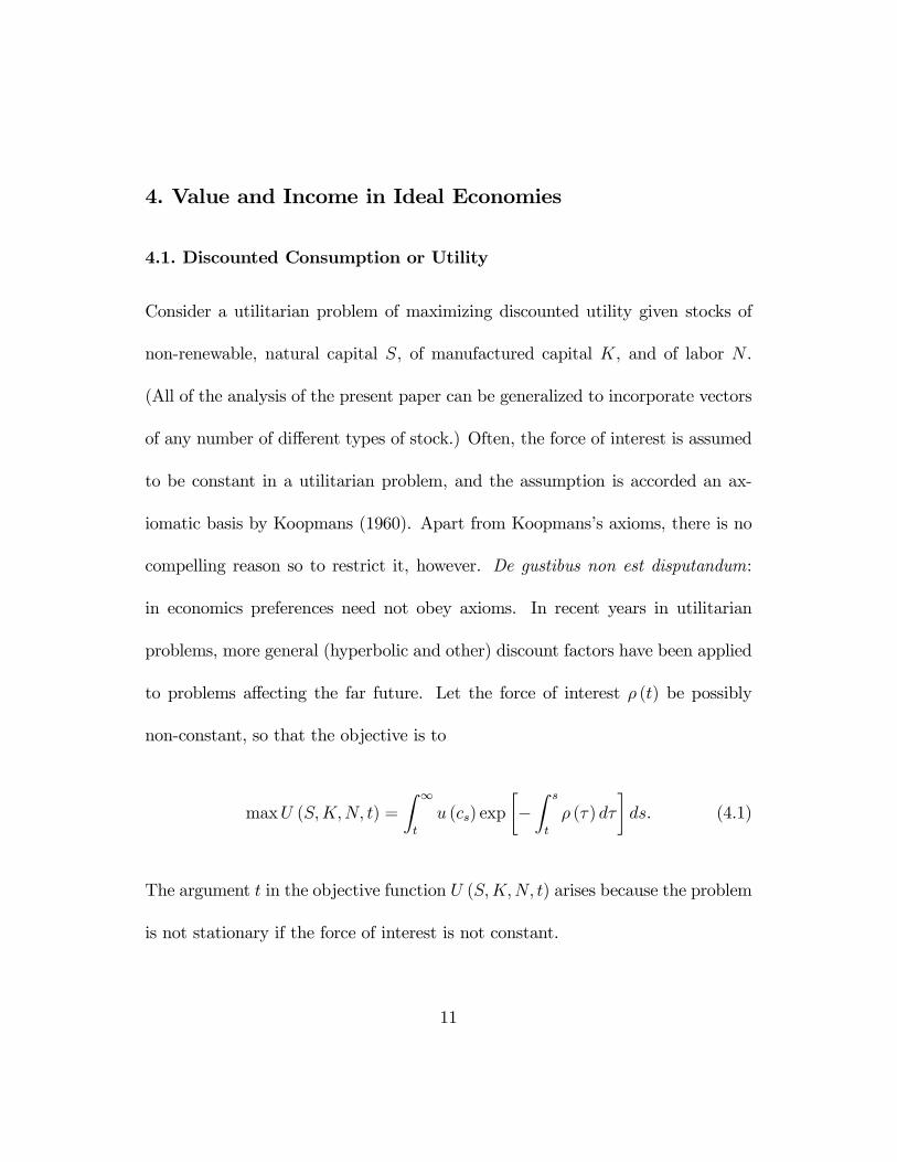
4. Value and Income in Ideal Economies

4.1. Discounted Consumption or Utility

Consider a utilitarian problem of maximizing discounted utility given stocks of

non-renewable, natural capital S, of manufactured capital K, and of labor N .

(All of the analysis of the present paper can be generalized to incorporate vectors

of any number of different types of stock.) Often, the force of interest is assumed

to be constant in a utilitarian problem, and the assumption is accorded an ax-

iomatic basis by Koopmans (1960). Apart from Koopmans’s axioms, there is no

compelling reason so to restrict it, however. De gustibus non est disputandum:

in economics preferences need not obey axioms. In recent years in utilitarian

problems, more general (hyperbolic and other) discount factors have been applied

to problems affecting the far future. Let the force of interest ρ (t) be possibly

non-constant, so that the objective is to

maxU (S,K,N, t) =

Z ∞

t

u (cs) exp

∙−Z s

t

ρ (τ ) dτ

¸ds. (4.1)

The argument t in the objective function U (S,K,N, t) arises because the problem

is not stationary if the force of interest is not constant.

11

The transition equations governing this system are

S (t) = −R (t) ;

K(t) = F (K,R,N)− c− δK; and

N = 0.

The current-value Hamiltonian for the problem is

HU = u (c)− λUR+ µU [F − c− δK] .

Necessary conditions for a maximum include:

u0 − µU = ∂HU/∂c = 0;

µUFR − λU = ∂HU/∂R = 0;

λU= ρλU − ∂HU/∂S = ρλU ;

µU = ρµU − ∂HU/∂K = µU (ρ+ δ − FK) .

Algebraic manipulation of these conditions yields Ramsey’s rule, linking the rate

of utility discount ρ, the rate of change of marginal utility u0/u0, and the net (of

12

deterioration) productivity of capital,

FK − δ = ρ− u0/u0.

It also yields the macroeconomic rendering of Hotelling’s rule, relating the rate of

change of the marginal productivity of the resource and the net marginal produc-

tivity of capital,

FRFR

= (FK − δ) . (4.2)

Consider now a perfectly competitive economy. The implicit objective is to

maximize the integral of consumption evaluated at present-value prices [ps]∞t

(prices into which the market discount factors are already incorporated), i.e. to

maxV (S,K,N, t) =1

pt

Z ∞

t

pscsds, (4.3)

subject to the same conditions. The present-value Hamiltonian is

HV = pc+ µV [F − c− δK]− λVR.

13

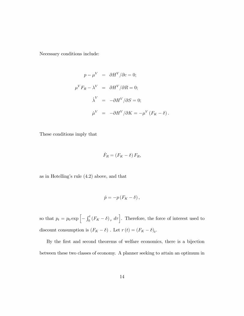
Necessary conditions include:

p− µV = ∂HV /∂c = 0;

µV FR − λV = ∂HV /∂R = 0;

λV= −∂HV /∂S = 0;

µV = −∂HV /∂K = −µV (FK − δ) .

These conditions imply that

FR = (FK − δ)FR,

as in Hotelling’s rule (4.2) above, and that

p = −p (FK − δ) ,

so that pt = p0 exph−R t0(FK − δ) τ dτ

i. Therefore, the force of interest used to

discount consumption is (FK − δ) . Let r (t) = (FK − δ)t.

By the first and second theorems of welfare economics, there is a bijection

between these two classes of economy. A planner seeking to attain an optimum in

14

problem (4.1) can decentralize present-value prices pt = u0 (ct) exph−R t0r τ dτ

i=

µU exph−R t0r τ dτ

i= µV and (pFR)t = λVt = λUt exp

h−R t0r τ dτ

i. At these

prices, ρ − u0/u0 = FK − δ = r. (If at any time u is changing, then r 6= ρ and if

u is constant then r = ρ.) The two economies follow the same path. Since there

are economies with objective (4.3) that correspond to economies with objective

(4.1), there is good reason to let the force of interest vary in the latter.

Along the optimal path that is the explicit solution for problem (4.1) and

implicit for problem (4.3), differentiation in two ways yields

ρU − u (c) = U = K∂U/∂K + S∂U/∂S + ∂U/∂t = µK + λS + ∂U/∂t.

The term ∂U/∂t arises because of non-stationarity, i.e., exogenous changes of

preferences, technology or other underlying conditions. In the present problem,

the force of pure time preference, ρ, is allowed to change; if ρ is constant then

∂U/∂t = 0. Let u0 (c) + cu0 (c) = u0 (c) + pc = u (c) at time t, and identify u0 (c)

as aggregate consumers’ surplus. Then

ρU − ∂U/∂t = H = u+ µK + λR = u0 + pc+ pK + (pFR) S.

15

Except for the term ∂U/∂t, interest (at the pure rate of time preference ρ) on

wealth U is equal to NNP at market prices, pc + pK + (pFR) S, plus aggregate

consumers’ surplus, u0. The last is not easily measured and depends on the point

on the utility surface.

(One can also, purely formally, define time t as a state variable of the problem

with t = 1 and shadow price q = ∂U/∂t. In this case the Hamiltonian of the

problem would be u + µK + λR + q = H + q; it would be exactly interest on

wealth. This approach is not pursued herein.)

One can also write, for the implicit objective of problem (4.3),

rV − pc = dV/dt = K∂V/∂K + R∂V/∂R+ ∂V/∂t = pK + pFRS + ∂V/∂t. (4.4)

Therefore,

rV − ∂V/∂t = pC + pK + pFRS. (4.5)

Net national expenditure at market prices, pC + pK + pFRS, is equal to interest,

at the consumption rate of discount r, on value (or market wealth) V , minus the

drift ∂V/∂t.

Both problems illustrate Weitzman’s contribution. (See also Weitzman 2000.)

The Hamiltonian is (or approximates if the problem is not stationary so that

16

∂U/∂t 6= 0 or ∂V/∂t 6= 0) the current return on value. That is to say, it is (or

approximates) the force of interest applied to the value of the objective.

In defining NNP the statistician neglects u0 + ∂U/∂t, or neglects ∂V/∂t. If

time is truly shifting the value function, then the effect of time should be evaluated

and appear in statistics; a rower’s rate of progress in a stream depends on both

the level of exertion and the current. In reality there may be some drift. Whether

it is important is an empirical question. If the problem is comprehensive, in that

all sources of change are incorporated into some form of capital, then the term

∂U/∂t or ∂V/∂t occurs only because of changes in the force of interest. It may

be small, as the term structure of interest rates has remained in a narrow band

through time.

The neglect of aggregate consumers’ surplus u0 is the reason that (real) NNP

is only a first-order approximation to the Hamiltonian of problem (4.1). On a

personal note, I am sure that my own consumer’s surplus is finite, but have no

inkling of its level, let alone the world’s aggregate consumers’ surplus. I am

sympathetic to neglecting it in an economic statistic, especially in view of the

correspondence between problems (4.1) and (4.3) and of the practicality of the

resulting statistic.

A much more fundamental objection to NNP is that one may not concur

17

with the value implied by using a utilitarian objective in general, or with the set

of preferences U (S,K,N, t) and {ρt}∞t=0 that give rise to the particular implicit

objective to which a given competitive outcome corresponds.

4.2. Wealth vs. Income Accounting

When the force of utility discount is a constant, γ, Weitzman (2000) notes that

Ut =Htγ,

so that if Ht were available at all future times s, the value of Ut would be the

same: Z ∞

t

u(c)e−γ(s−t) ds = Ut =

Z ∞

t

Hte−γ(s−t) ds.

Weitzman calls Ht, which is the net national product, the stationary equivalent.

In the general case, the stationary equivalent is not attainable (lies outside the

utility-possibilities frontier). Even though Weitzman was at pains to stress that

the stationary equivalent may not be sustainable, occasionally it is misinterpreted

as a measure of sustainable consumption. It is a mathematical curiosum that

holds only for a constant force of interest. The expression becomes messy if the

rate of utility discount is not constant. Let the force of utility discount be, as

18

above, ρt. The interpretation of Weitzman’s finding depends on the fact that

Ht = ρtUt,

so that the Hamiltonian (NNP) is interest on, and hence income from, value Ut.

This formulation is consistent with a Hicksian interpretation of NNP; the following

asset-equilibrium conditions for total value are exact:

rV = pc+ dV/dt;

ρU = u (c) + dU/dt.

Interest, at the appropriate rate, on value (be it V or U depending on the objective

being studied) is equal to the current dividend (pc or u (c)) plus the capital gain

(dV/dt or dU/dt). Interest on the economy’s value is its income.

Thus, value and income are sides of the same coin (Samuelson 1961). If con-

sumption pc or utility u (c) is equal to income, then value does not change. Hicks

(1946) assumes that an individual’s goal is to sustain consumption; the individual

has the maximin objective. In problems (4.1) and (4.3), however, maximin is not

the goal. If value is changing (if dV/dt or dU/dt is changing) then the dividend

19

that is being (optimally) consumed is greater or less than income.

Hicks’s notion of income can be applied in the context of a utilitarian economy

if one observes that the definition of income is not dependent on sustaining utility

or consumption. NNP is not an index of welfare or value; rather, it measures the

flow emanating from the stock of welfare.

4.3. Sustained Consumption or Utility

If an analyst wishes to study sustainability as a social value, then sustaining the

economy belongs in the objective. The solution (Cairns and Long 2001) of a

stationary maximin program is a level of utility υ that is sustained through time

and that is equal to an aggregate of the stocks,

υ = φ (S,K,N) .

The function φ indexes value, which is the minimum attained utility over all

time. Unlike in a utilitarian problem, in a maximin problem value is a flow, not

an aggregate on which interest is earned. Such an aggregate is not defined in a

maximin problem. Indeed, there is no interest rate. (There is a virtual interest

rate, but that rate is a derived, technical variable, not a preference using which

20

the analyst aggregates levels attained at different times into a measure of value.)

Society’s income at every point in time is also the minimum attained level of

utility, in this case also its value. This observation coincides with Hicks’s for an

individual maximizing sustained utility.

If φ is differentiable then

∂φ

∂SS +

∂φ

∂KK +

∂φ

∂NN =

∂φ

∂SS +

∂φ

∂KK =

dφ

dt=dυ

dt= 0. (4.6)

Hartwick’s rule (4.6) (Hartwick 1977) is that at any time total net investment,

evaluated at the shadow prices of a maximin problem, is zero. The expression

qSS + qKK is the Hamiltonian in a maximin problem, and in the solution qS =

∂φ/∂S and qK = ∂φ/∂K.

In the competitive economy postulated by Dixit et al., Hartwick’s rule is said

to hold. This is not to say, however, that the rule is defined in a market economy.

In their model the maximin problem has implicitly been solved to determine the

shadow values of equation (4.6) and then those (relative) shadow values, incorpo-

rating the appropriate virtual discount factors, have been decentralized. In this

specific competitive economy, the net value of investment is equal to zero at all

times.

21

If sustaining the economy is the social value (if the objective is to sustain

consumption or utility), net national product is not a useful statistic. The virtual

Hamiltonian from the virtual utilitarian problem does not have the meaning that it

has in an explicit utilitarian problem. A willingness to exchange utility at different

times at shadow prices λ (s), which is implied by writing down the utility integral

or the Hamiltonian, is incompatible with the analyst’s postulated preferences.

A maximin problem gives rise to two distinct statistics, the level of utility,

which remains constant, and the values of net investments in all stocks, which

are such that total net investment remains equal to zero. There is no theoretical

basis to add them to form NNP as in a discounting problem. Computing such a

sum is pointless. On the optimal maximin path, since aggregate net investment

is always equal to zero, NNP never changes as it is always equal to consumption.

Off the optimal path, the shadow values ({pt} and {λt}) have no interpretation.

4.4. NNP and Sustainment

The concept of income is at the heart of green accounting. Studying the problem of

sustaining an economy “as if” it were a utilitarian problem like problem (3.2) has

provided many insights. But the two problems are not identical. They express

different values, have different objectives, and hence have different concepts of

22

income.

Sustaining an economy is a long-run objective: the economy’s value must be

maintained forever. Solving a maximin problem gives the short-run conditions,

including Hartwick’s rule, for sustainment. The method of solution guarantees

that these conditions hold at each point on the maximin path. Solving a general,

utilitarian problem gives short-run conditions that may look like Harwick’s rule

but may not hold forever along the optimal path.

By choosing an objective to study, the analyst imposes a concept of value.

The main problem with trying to apply extended NNP to measure sustainment of

an economy is that use of NNP implies a social objective or value that is different

from sustainment. The difference has implications for the usefulness of NNP.

NNP is the (linearized) Hamiltonian of a utilitarian optimization problem

(evaluated with given discount factors). Even if sustainment is the analyst’s intent

and a discounted-utility problem is used as a vehicle for deriving properties of the

solution, the utilitarian problem is written as in equation (3.2). The discussion of

the maximin program above, however, indicates that the discount factors, λ (t),

are defined only on the maximin path. In order to find the discount factors, the

maximin problem must be solved. Moreover, writing down equation (3.2) implies

that any point on the hyperplane separating the production-possibilities frontier

23

from the objective makes the same contribution to value. When u (s) 6= u, s ≥ t,

it is inappropriate to writeR∞t

λ(s)λ(t)u (s) ds. It is appropriate to write this integral

only in a utilitarian problem in which {λ (s)}∞t is predetermined (exogenous to

the problem).

On the maximin path (the only path on which {λ (s)}∞t is defined),

Z ∞

t

λ (s)

λ (t)u (s) ds =

Z ∞

t

λ (s)

λ (t)uds = u

Z ∞

t

λ (s)

λ (t)ds = u;

the integral collapses to the maximin objective, u = maxu such that u (s) ≥ u.

By Hartwick’s rule, net investment is always zero; there is no point in reporting

net investment as a statistic or part of a statistic (NNP). Off the optimal path,

the shadow values have no interpretation: The inappropriateness of writing the

integral carries over to the Hamiltonian and hence to NNP. In short, when the

prices have meaning, nothing is gained by computing the investment component;

only consumption is a useful statistic.

If society’s real objective is not to sustain utility, it is well-known that keeping

net investment at zero (interpreted as following Hartwick’s rule, which usually

implies moving off the path that is optimal for the utilitarian objective) at the

given point in time does not imply sustainability. That is to say, for a general

24

utilitarian objective, setting net investment to zero is myopic. Hartwick’s rule

has to apply at each future point for utility to be sustained. The only utilitarian

objective for which this property holds is the one that coincides with the maximin

solution. As we have noted, even for this problem, NNP is not a useful statistic.

An optimal utilitarian path is Paretian. One criticism of maximin programs is

that, if a problem is not regular, if it is not possible to “spread” utility equally to

all points on the maximin path, the problem is not Paretian. That is to say, the

maximin value is the minimum level of utility on the path, and the greater levels

of utility at other points do not ‘count’ and the excess can be thrown away. The

reason, of course, is that a maximin program treats equality among generations

as the social value. No matter how defined, however, even with use of a utilitarian

welfare functional, attempting to impose a condition of intergenerational equity

must throw up non-Paretian cases. The criterion for sustainment on a utilitarian

path is often held to be whether utility is increasing (whether u ≥ 0) or else

whether value is increasing (whether V ≥ 0 ). If there are constraints preventing

the spreading of consumption equally in an economy, it may not be possible

always to have u ≥ 0 or V ≥ 0. The imposition of one of these conditions as a

constraint renders the sustainment problem non-Paretian as well. Furthermore,

the utilitarian formulation with the constraint is not a complete set of preferences,

25

as it does not distinguish among paths that have the same present value, in which

value is not decreasing but in which the rate of change of value is not the same.

Consider a fishery with a stock S. Let the harvest be H, and let S =

S (1− S) − H be the transition equation. The maximin level of consumption

is S (0) if S (0) ≤ 1/2, and 1/2 if S (0) ≥ 1/2. Let the initial stock be S0 > 1/2.

Imposing the constraint that u (0) ≥ 0 or that V (0) ≥ 0 (with any set of discount

factors) requires thatH = 1/2, when it could be greater early in the program. The

level of harvest is not Pareto optimal. Maximin does not have this requirement.

Consider a path on which consumption (be it optimal according to some cri-

terion or not) fluctuates about a rising, linear trend,

C (t) = A [1 + α sin (ωt+ β)] +Bt, (4.7)

so that the change in consumption,

C (t) = Aαω sin (ωt+ β) +B,

has the sign of B − αωA sin (ωt+ β). If B < Aαω then C (t) < 0 on regular

intervals, over which Aαω sin (ωt+ β) falls at a rate greater than B. Is this type

26

of path an “unsustained development”?

Now let this consumption path be discounted at some discount rate, r. With-

out loss of generality we can let ω = 1 and β = 0. Present value is

V (t) =

Z ∞

t

[A (1 + α sin s) +Bs] e−rtdt

=A

r+

Aα

1 + r2(cos t+ r sin t) +

B

r2(1 + rt) .

V (t) =Aα

1 + r2(− sin t+ r cos t) + B

r.

If t = ±2nπ,

V (t) =B

r− Aα

1 + r2

and so if

B < Aαr

1 + r2( < Aα), (4.8)

there are regularly repeated intervals on which V (t) < 0. The value function,

however, never falls below

A

r− Aα

1 + r2+B

r2,

and we can make this arbitrarily close to A/r (and A/r arbitrarily large) while

satisfying condition (4.8). Value eventually grows like (B/r) t. There is an ε

27

(small) for which V (t) > Ar− ε for all t, even if V (t) < 0 for some values of t,

perhaps the current value. Is this an unsustained economy?

The problems just raised are why the literature has derived many contradic-

tory and conflicting definitions and concepts of sustainable utility starting from a

utilitarian value function. The only advantage of this objective function over the

direct formulation of maximin is its familiarity.

Thus far, discussion has been limited to optimal programs. The fundamental

reason why accounts are needed is that the economy is not optimal. A real

economy does not maximize an explicit objective. What are to be used as value

and income in a real economy, for which we must produce real statistics?

5. Value and Income in a Real Economy

5.1. Ideal Valuation

One is entitled, if not obliged, to challenge the outcome of any real economy

in terms of values that are of interest to the analyst. Such an evaluation is a

possible interpretation of Dasgupta and Mäler’s (2000: 83 ff.) discussion of social

well being and the concept of sustainability. They present a model of a real

economy following some observed path through time. The economy’s institutions

28

and policies are represented by a vector, α. We can generalize their postulated

expression of value as

V R (K, t |α) =Z ∞

t

δ (s) u α (cs) ds. (5.1)

(In a completely general accounting system, the institutions and policies could

form a sub-vector of the vector of the economy’s capital stocks, K.) Dasgupta

and Mäler make no mention of maximizing value, V R (K, t |α); they derive no

Ramsey condition related to α. A small policy change Oα is contemplated, but it

need not be optimal, nor indeed even an improvement.

The problem expresses what the authors wish to examine as value; they could

as reasonably have chosen as the measure of value the level of utility of the genera-

tion living at some time t0, or the level of utility of the generation with lowest (in-

fimum) utility. In the context of a value function having the form of V R (K, t |α),

it is still possible to challenge the values inherent in the utility function uα (c)

or the discount factors δ (t). The main property of NNP is that its form is the

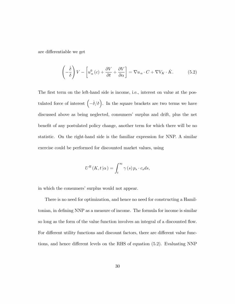
same, whatever the particular choices of uα or δ. If both sides of equation (5.1)

29

are differentiable we get

Ã− δ

δ

!V −

∙u0α (c) +

∂V

∂t+

∂V

∂α

¸= ∇uα · C +∇VK · K. (5.2)

The first term on the left-hand side is income, i.e., interest on value at the pos-

tulated force of interest³−δ/δ

´. In the square brackets are two terms we have

discussed above as being neglected, consumers’ surplus and drift, plus the net

benefit of any postulated policy change, another term for which there will be no

statistic. On the right-hand side is the familiar expression for NNP. A similar

exercise could be performed for discounted market values, using

UR (K, t |α) =Z ∞

t

γ (s) ps · csds,

in which the consumers’ surplus would not appear.

There is no need for optimization, and hence no need for constructing a Hamil-

tonian, in defining NNP as a measure of income. The formula for income is similar

so long as the form of the value function involves an integral of a discounted flow.

For different utility functions and discount factors, there are different value func-

tions, and hence different levels on the RHS of equation (5.2). Evaluating NNP

30

requires shadow values, ∇uα and ∇VK , and hence some at least implicit knowl-

edge of V (K, t |α), as well as a fore-knowledge of how any increase in a component

of the vector K will be deployed.

5.2. NNP at Market Prices

Even a distorted economy may be viewed as behaving as if having some im-

plicit objective similar to that of the hypothetical perfectly competitive economy

(Cairns 2002b). According to the separation theorem, which separates decisions

on investment from those on allocation of consumption, the objective, which need

not be viewed as being maximized, is market wealth. Let the technology be as

in problems (4.1) and (4.3). At time s, let the market force of interest be repre-

sented by rs and the present-value price of the consumption good by πs (so that

πs/πs = rs and hence πt = π0 exp³R t

0rs ds

´). Market wealth is

W (S,K, t) =

Z ∞

t

πsπtcsds. (5.3)

31

Let Y represent current NNP and let S∂W/∂S + K∂W/∂K, net investment, be

represented by I.1 If W (S,K, t) is differentiable, then differentiating it in two

ways and a then further differentiation yield

W (S,K, t) = S∂W/∂S + K∂W/∂K + ∂W/∂t; (5.4)

rW = c+ W = Y + ∂W/∂t; (5.5)

Y = rW + rW − d/dt (∂W/∂t) . (5.6)

If the exogenous drift in the economy (accounting for ∂W/∂t) and in the force

of interest (r) are equal to zero–heroic assumptions in a real economy–equations

(5.4) and (5.6) imply that

sgnY = sgnW = sgnI: (5.7)

1The asset value of the resource is the discounted value (at rate rt) of its earnings,

At =

Z ∞t

πRFR exp

µ−Z s

t

r τ dτ

¶ds.

The depreciation of this value is −A = πRFR−rA; it is the change in income from the resource,and is net investment on the income side of the green accounts. On the expenditure side,net investment is −πRFR, the component of the Hamiltonian corresponding to changes in thequantity of the resource. Cairns (2002a) presents a detailed discussion. The expression S∂W/∂Scorresponds to πRFR.

32

At any time, each of market income or green NNP (Y ) and market wealth (W )

moves in the direction of the market value of net investment. Equation (5.7) is a

net-investment rule in a market economy. (If the problem is non-stationary, the

rule is only approximately true.) This net-investment rule uses observed or at

least potentially observable statistics. The statistic, NNP at market prices, is a

measure of achieved performance, not optimal or potential performance.

Manipulation of equations (5.5) and (5.4) yields that

c = rW − W = rW − I − ∂W/∂t.

By differentiation and then substitution from equation (5.4),

c = rW + rW − I − d

dt

∂W

∂t

=³rI − I

´+ rW +

µr − d

dt

¶∂W

∂t.

If r = 0 and ∂W/∂t = 0, then (cf. Hartwick 2003)

sgn c = sgn³r − I/I

´. (5.8)

Equation (5.8) provides a local indicator of the rate of change of consumption. It

33

is not a measure of sustainability of consumption, nor even of local sustaining of

consumption, as these require global solutions.

5.3. Sustaining a Decentralized Economy

Consider an ideal, competitive economy or a real, market economy. For appro-

priate present-value prices [ps]∞s=t, or for appropriate current-value prices [vs]

∞s=t

and discount factors [βs]∞s=t, the economy is implicitly maximizing a utilitarian

objective,

Φt =

Z ∞

t

ps · cs ds =Z ∞

t

(βsvs) · cs ds.

Let the prices satisfy all the conditions enunciated by Dixit et al. for a regular

path,2 and also let it be feasible for the economy to follow a sustainable path.

Suppose that an onlooker wishes to evaluate whether the economy is being

sustained. (The onlooker, then, rejects the implicit, utilitarian objective of the

economy and has the maximin objective.) Unless the prices [ps] or [βsvs] are such

that this economy happens to be following a constant-utility path for all time,

the prices are not relevant for the onlooker’s evaluation. Observed, market prices

are not “right” for determining whether an alternative objective is being followed;

2Regularity narrows things down but not very far. There are an uncountably infinite numberof regular paths, only one of which is a constant-utility path.

34

rather, if there is an alternative objective to “what the economy is implicitly

maximizing” (for which market prices are the appropriate shadow values), the

prices used should be the shadow prices for that objective. Conceptually, the

onlooker can determine whether the economy is on the sustainable path at time

t, given its endowment of stocks, by solving the maximin problem (3.1) to find

the shadow values of the stocks at time t. These shadow values can be applied

to the net investments, according to Hartwick’s rule (4.6). The sign of total, net

investment is descriptive of the economy: If the sum is zero, then the economy is

being sustained at time t.

If the sum is negative, the economy is not being sustained. If the sum is

positive, the economy is “more than” being sustained. If the sum is non-zero on

an interval, however, the economy is taken off the maximin path and the prices

no longer have the interpretation of shadow prices for the maximin problem. The

evaluation can no longer be made.

Mathematically, there do exist current prices for evaluating whether the econ-

omy is being sustained at time t. They are the right prices for time t, irrespective

of whether the decision makers of the present or the future decide to sustain or

not to sustain the economy. It is impractical to think that the shadow prices could

be determined for a real economy.

35

For the economy actually to be sustained for all future time from time t,

Hartwick’s rule must be followed at all times s ≥ t, using the shadow prices

for those times. The maximin solution prescribes Hartwick’s rule, and so the

net-investment rule for a sustained economy is prescriptive.

In a steady state, since the rate of change of each stock is zero, Hartwick’s rule

is trivially satisfied. A steady state is perhaps a naive ecologist’s dream. It implies,

however, ecological stagnation. An ecologically vibrant, sustained economy must

have positive shadow prices, so that some stocks are rising and some falling. Stocks

are substituting for each other in producing the constant level of utility through

time. Ecological sustainment is not possible without substitution.

6. Conclusion

The objective in a theoretical model is the theorist’s postulate of the meaning

of value, and the outcome of the model yields a representation of value and of

income. It is not consistent to use that model to consider other concepts of value

or income. The net-investment rule is no guide for sustaining an economy when

market prices are the basis of evaluating net investments. Rather, if the objective

is to maximize sustainable consumption, the analyst must solve an overwhelmingly

complex maximin problem to obtain the shadow prices of investments for use in

36

Hartwick’s rule. Theoretically, in both coverage and relative prices, sustainability

accounts entail a complete break from the national accounts. Consequently, they

are impractical.

It is vital to understand the meaning of environmental accounting and what it

can accomplish for society. As Nordhaus and Tobin observed over thirty years ago,

using techniques of non-market valuation to incorporate unpriced environmental

flows can improve NNP as an indicator of utilitarian value. The interpretation is

founded on discounting, which is an unappealing feature to many. No explicit op-

timization of a value function is required or contemplated, however. If there are

important divergences from perfect competition, market prices are still shadow

prices for a virtual value function, for whatever “the market is implicitly maxi-

mizing,” subject to all the practical constraints facing a real economy. Extending

NNP at market prices in the intent of providing an income-based indicator of

welfare implies acceptance of that virtual value. Acceptance of the market out-

come may be even less appealing than acceptance of discounting. Still, economists

can make the case that if growth, defined as increasing green NNP consistently

through time, is successful, then environmental quality and other features of the

quality of life will almost surely continue to improve, because they are normal

goods.

37

References

[1] Burmeister, Edwin and Peter J. Hammond (1977), “Maximin Paths of Het-

erogeneous Capital Accumulation and the Instability of Paradoxical Steady

States,” Econometrica 45, 4, 853-870.

[2] Cairns, Robert D. (2000), “Sustainability Accounting and Green Account-

ing,” Environment and Development Economics 5, 1&2, Feb. & May, 49-54.

[3] Cairns, Robert D. (2002a), “Green National Income and Expenditure,”

Canadian Journal of Economics 35, 1-15.

[4] Cairns, Robert D. (2002b), “Green Accounting Using Imperfect, Current

Prices”, Environment and Development Economics 7, 207-214.

[5] Cairns, Robert D. and Ngo Van Long (2001), “Maximin: A New Approach,”

presented to the meetings of the European Association of Environmental and

Resource Economists, Southampton UK, June.

[6] Dasgupta, Partha and Karl-Goran Mäler (2000), “Net National Product,

Wealth and Social Well Being,” Environment and Development Economics

5, 1&2, Feb. & May, , 69-94.

38

[7] Dixit, Avinash, Peter Hammond and Michael Hoel (1980), “On Hartwick’s

Rule for Regular Maximin Paths of Capital Accumulation and Resource De-

pletion,” Review of Economic Studies 47, 551—556.

[8] Hartwick, John (1977), “Intergenerational Equity and the Investing of Rents

from Exhaustible Resources,” American Economic Review 66, 972-974.

[9] Hartwick, John (2003), “Net Investment and Sustainability,” Natural Re-

source Modeling 16,2.

[10] Hicks, John R. (1946) Value and Capital, Second ed., Oxford UP.

[11] Koopmans, Tjalling C. (1960), “Stationary Ordinal Utility and Impatience,”

Econometrica 28, 287-309.

[12] Nordhaus, William D. and James Tobin (1972), “Is Growth Obsolete?” in

Economic Growth, Fiftieth Anniversary Colloquium, National Bureau of Eco-

nomic Research, Columbia UP, New York.

[13] Rawls, John (1971), A Theory of Justice, Harvard UP, Cambridge MA.

[14] Solow, Robert M. (1974), “Intergenerational Equity and Exhaustible Re-

sources,” Review of Economic Studies 41, 29-45.

39

[15] Weitzman, Martin L. (1976), “On the Welfare Significance of National Prod-

uct in a Dynamic Economy,” Quarterly Journal of Economics 90, 156-162.

[16] Weitzman, Martin L. (2000), “The Linearised Hamiltonian as Comprehensive

NDP,” Environment and Development Economics 5, 1&2, Feb. & May, , 55-

68.

40