1 Value Investing: Cheapness, Quality, and Investor Confidence* Benjamin Maury Hanken School of Economics This version: April 23, 2015 Abstract This paper investigates whether signals from changes in investors’ portfolio concentrations can be used to enhance the performance of value and value/quality stock portfolios. Using data on all the more than 1.3 million investor portfolios participating in the Finnish stock market, I find that increases in average shareholder portfolio concentration, a signal of investor confidence, can be used to improve the performance of value portfolios and portfolios selected based on value and quality signals. The results indicate that shareholder portfolio concentration can be used as an additional signal to improve the performance of value-oriented investing strategies. Keywords: Value investing, quality investing, portfolio concentration, ownership concentration, quality at reasonable price, stock returns. JEL Classification: G11, G14, G32. * Department of Finance and Statistics, Hanken School of Economics, P.O. BOX 479, 00101 Helsinki, FINLAND. E-mail: [email protected]. Phone: +358405489847. I am grateful to Anders Löflund, Per Strömberg, and workshop participants at Hanken School of Economics (2013) for valuable comments. Financial support from OP- Pohjola Research Foundation is gratefully acknowledged.
Transcript
1
Value Investing: Cheapness, Quality, and Investor Confidence*
Benjamin Maury
Hanken School of Economics
This version: April 23, 2015
Abstract
This paper investigates whether signals from changes in investors’ portfolio concentrations can be used to enhance the performance of value and value/quality stock portfolios. Using data on all the more than 1.3 million investor portfolios participating in the Finnish stock market, I find that increases in average shareholder portfolio concentration, a signal of investor confidence, can be used to improve the performance of value portfolios and portfolios selected based on value and quality signals. The results indicate that shareholder portfolio concentration can be used as an additional signal to improve the performance of value-oriented investing strategies.
Keywords: Value investing, quality investing, portfolio concentration, ownership concentration, quality at reasonable price, stock returns.
JEL Classification: G11, G14, G32.
* Department of Finance and Statistics, Hanken School of Economics, P.O. BOX 479, 00101 Helsinki, FINLAND. E-mail: [email protected]. Phone: +358405489847. I am grateful to Anders Löflund, Per Strömberg, and workshop participants at Hanken School of Economics (2013) for valuable comments. Financial support from OP-Pohjola Research Foundation is gratefully acknowledged.
2
1. Introduction
This paper explores whether shareholder portfolio holding data can be used to improve the
performance of value portfolios. While quality variables, such as profitability, financial strength,
and quality more generally (Novy-Marx, 2013; Piotroski, 2000; Asness et al., 2014;
respectively), have been shown to enhance the performance of value portfolios selected based on
valuation multiples, portfolio concentration and ownership data have not been used in value
studies or studies combining value and quality dimensions. This paper aims to fill the gap in the
literature.
Previous empirical research finds that value stocks (e.g., high book-to-market) have
performed better than growth stocks in the US (Fama and French, 1992; Lakonishok, Shleifer,
and Vishny, 1994; La Porta, Lakonishok, Shleifer and Vishny, 1997) as well as internationally
(Fama and French, 1998). Moreover, Piotroski (2000) shows that measures of financial strength
can be used to separate winners form losers within portfolios of value stocks. Relatedly, Novy-
Marx (2013, 2014) finds that quality variables (such as gross-profitability divided by total assets)
can be used to improve the performance of value portfolios. Furthermore, Novy-Marx (2014)
and Piotroski and So (2012) show that value and quality sorting strategies based on combined
ranks perform better than a 50/50 combination of value and quality portfolios.
In this paper, I consider the usefulness of investor portfolio concentration data in selecting
value stocks. Ekholm and Maury (2014) find that shareholder portfolio concentration is
positively related to future firm performance. Their results are consistent with the idea that
concentrated portfolios improve price efficiency which in turn improves managerial decision-
making. The results on stock returns in Ivkovic et al. (2008) as well as Ekholm and Maury
(2014) suggest that focused investors are more informed than more diversified investors and that
information on portfolio concentrations can be a valuable signal on future stock performance.
3
Thus, previous research would indicate that portfolio concentration data could be used to
improve the selection stocks with the high expected returns within a value investing strategy.
Using data on virtually every investor’s portfolio holdings in the Finnish market over the
period 1996-2005, I employ the portfolio concentration index developed in Ekholm and Maury
(2014) which is measured as the average portfolio weight of all shareholders in a firm. The
portfolio concentration measure is used as a signal of confidence in the quality of a stock. Two
main empirical approaches are employed in this paper. In the first approach, the portfolio
concentration index is combined with a value portfolio. In the second approach, portfolio
concentration data are combined with a portfolio formed based on combined value and quality
ranks.
The results show that information on changes in portfolio concentration can be valuable
when used in combination with value-oriented investment strategies. First, portfolio
concentration data can be used directly to select the best performing stocks within a value
portfolio (i.e., to avoid the so-called value trap). Second, portfolio concentration can be used as a
third variable in combination with value and quality variables to obtain higher stock returns. The
findings indicate that portfolio concentration data can further enhance the performance of
portfolios formed on a combination of quality and value variables. Moreover, portfolio
performance is higher when the average portfolio concentration is calculated for larger (such as
at least 0.1% or 1% holdings), and presumably more informed, shareholders. In addition, I find
that increases in ownership concentration can be used as an alternative investment signal,
although the portfolio performance using ownership concentration data is lower than the
performance using information on portfolio concentrations. Taken together, the empirical
findings in this paper indicate that data on investors’ portfolio holdings can be used as a signal
that adds to the performance of investment strategies based on value as well as combinations of
value and quality without increasing known portfolio risk.
4
This paper is related to two main strands in the literature. The first strand on investment
research has shown that value portfolios (e.g., Fama and French, 1992) and portfolios that
combine value and quality (e.g., profitability or financial strength) signals (e.g., Novy-Marx,
2013; Piotroski, 2000; Asness et al., 2014) have generated returns in excess of the market.
Another strand in the literature studies the usefulness of holdings data for investment purposes.
Regarding insider trades, Jaffe (1974), for example, finds that returns to stocks purchased
slightly after insiders’ purchases have become public information generate returns significantly
higher than that of the market. Relatedly, Kallunki et al. (2009) find that insider selling is
informative among those insiders that have the highest proportion of their wealth concentrated in
insider stocks. More generally, Ekholm and Maury (2014) find that the average shareholder
portfolio concentration is positively related to future profitability, valuations, and stock returns,
which is consistent with both monitoring through the stock market and superior stock selection
ability by more focused shareholders. While these previous papers consider the investment
returns utilizing holdings data, they do not analyze whether holdings data can be useful as an
additional signal that could complement value and quality sorts. This paper contributes to the
existing literature by showing that investor portfolio data can be used to improve the returns on
value-oriented portfolios.
Although this paper uses data available on Finnish listed firms, the findings in this
paper are likely to be relevant for international investors due to the following reasons. Firstly,
information on holdings data and portfolio concentration could be obtained for other markets
than the Finnish market used here. For example, data from 13F filings provided by Thomson
Financial that cover institutional investors who manage more than $100 million could be
obtained for US firms. These data could be used to calculate a proxy for the AWI (portfolio
concentration) measure. Secondly, the findings in this paper indicate that also ownership
concentration data, more accessible and easily computed, can be used to improve returns.
5
The paper proceeds as follows. Section 2 reviews previous research and presents the
hypotheses. Section 3 describes the data set. Section 4 presents the empirical findings as well as
offers alternative models and robustness tests. Section 5 concludes the paper.
2. Value investing and holdings data
In this section, I review previous literature on value investing and discuss the usefulness
of combining information on holdings data (especially shareholder portfolio concentration data)
with value and quality investing strategies.
2.1. Value portfolios
Prior research finds that value stocks (e.g., high book-to-market stocks) outperform
where Return is the market-adjusted annual return for the period (May year t to April year t+1),
Ln(Book-to-Market) is the natural logarithm of the Book-to-Market ratio, Ln(MVE) is the
natural logarithm of the market capitalization of equity (both variables are measured at end of t-
19
1)16, Momentum is the past 6 month stock return directly prior to portfolio formation,17 and ε is
the error term.18 Other variables are defined in Section 3.
The results from pooled OLS regressions in which standard errors control for firm and
year clustering (see Petersen, 2009, Gow et al. 2010, and Dickinson and Sommers, 2012) are
displayed in Table 4.19 The sample used in the regressions consists of value firms defined as
firms with book-to-market ratios above the median value each year. Table 4 shows that the
coefficient for changes in portfolio concentration (ΔAWI) for 0.1% and 1% shareholdings is
significantly positively related to one-year market-adjusted stock returns at the 1 % level, while
the coefficient for ΔAWI for all shareholdings is positive but statistically significant only at the
10% level. Taken together, the regressions indicate that the signal from changes in shareholders’
portfolio concentration is not explained by previously known return patters. Thus, the regressions
give support to the results from the portfolio approach in Section 4.2.1.
4.2.3. Portfolio risk
16 Besides controlling for the size effect, market capitalization is an important control variable since the relation
between market capitalization and portfolio concentration may be non-trivial as price increases also can increase
portfolio concentration.
17 I use the six month return directly prior to portfolio formation following Piotroski (2000), Mohanram (2005), and
Piotroski and So (2012).
18 To maintain sample size, the momentum variable is set equal to zero for missing observations. The regression
model includes a dummy variable which is equal to one if the momentum data was available and zero otherwise.
19 The results are qualitatively similar when Fama-Macbeth Newey-West standard errors that control for
autocorrelation are used as in Piotroski and So (2012).
20
In this section, I discuss levels of risk-related measures for the various portfolios formed
based on value, quality, and changes in portfolio concentration.20 To further explore whether
higher portfolio performance is associated with a compensation for higher risk (e.g., Fama and
French, 1992), I follow Mohanram (2005) and estimate CAPM betas (β). In addition, I measure
the standard deviation of past 5-year ROA.
Panel A of Table 5 shows that the systematic risk measured by CAPM β (column 1) and
the standard deviation of the 5-year ROA (column 2) are significantly lower for the value than
for the glamour portfolio. Panel B shows that value firms with high ΔAWI values have
somewhat lower risk levels compared with all value firms in Panel A. Similar risk patterns are
found for portfolios sorted based on value and quality ranks in combination with ΔAWI for all or
1% shareholders (Panels D and E). Taken together, the results in Table 5 indicate that the
portfolios associated with high stock performance (in Tables 2 and 3) generally exhibit lower
risk than in the lower performance portfolios. The results in Table 5 support the mispricing
explanation but not the explanation holding that return is a reward for risk.
4.3. Further analysis
This section discusses how the main results are affected by (i) the use of F-score as a
quality variable, (ii) alternative partitions of the data regarding value/growth portfolio cut-offs,
firm size, share turnover, and analyst coverage, (iii) the timing of the use of portfolio
concentration data (e.g., using ΔAWI in the first sorting stage versus the last stage), as well as
(iv) alternative timings of accounting data and stock returns (e.g., further lagged accounting
data), and alternative return periods.
20 This section on risk measures complements the risk-adjusted portfolio performance analysis using Jensen (1968)
alpha and Carhart (1997) four factor alphas in Section 4.2.1.
21
4.3.1. F-score as quality measure
As an alternative to the ROA measure, I consider Piotroski’s (2000) F-score as a quality
measure. The F-score measures firms’ financial strength by using nine financial variables that
can be grouped into three key areas: profitability, financial leverage/liquidity, and operational
efficiency (see, Piotroski, 2000, for details). The aggregate of the nine binary variables is the F-
score. Data used to calculate the nine binary variables that form the aggregate F-score are
obtained from Thomson Financials except for the equity issue variable that is based on the year
book Pörssitieto.
Panel A of Tables 6 shows the results for a portfolio that contains high book-to-market
firms (Q3, Q4) with high F-score firms (Q3, Q4). The results show that the F-score sort improves
the pure value strategy presented in Table 2. Moreover, Panel B of Table 6 shows that
partitioning the high F-score / value portfolio based on investor portfolio concentration (high
concentration) further improves portfolio performance on a risk-adjusted basis. The returns of
the high-low F-score/value/ΔAWI portfolio equal 14% on average using market-adjusted returns
(column 2). Taken together, information from portfolio concentration appears to enhance the
performance of the Piotroski (2000) method. Also, the performance of the Piotroski-AWI screen
is comparable with the profitability-AWI screen (Table 2).
4.3.2. Alternative data partitions
In this section, results using different definitions for value and glamour firms, as well as
controlling for firm size, share turnover (liquidity), and analyst coverage (for a discussion of
these partitions see Piotroski, 2000) are discussed. I consider alternative partitions for value and
22
glamour firms (similarly for high and low combined value and quality portfolios) in which value
firms are those with above median book-to-market ratios and glamour firms are those with book-
to-market ratios equal to or below median levels. As displayed in Panels B and C of Table 6,
such definitions of value and glamour stocks yield rather similar results as compared with the
results in the main specifications based on quartiles. Furthermore, I also partitioned the sample
into stocks with equal to or above median and below median firm size (measured by the market
capitalization of the firm). Again the main results are rather similar for large and small firms,
although larger firms tend to exhibit somewhat higher portfolio performance for the sample
stocks (Panels D and E).
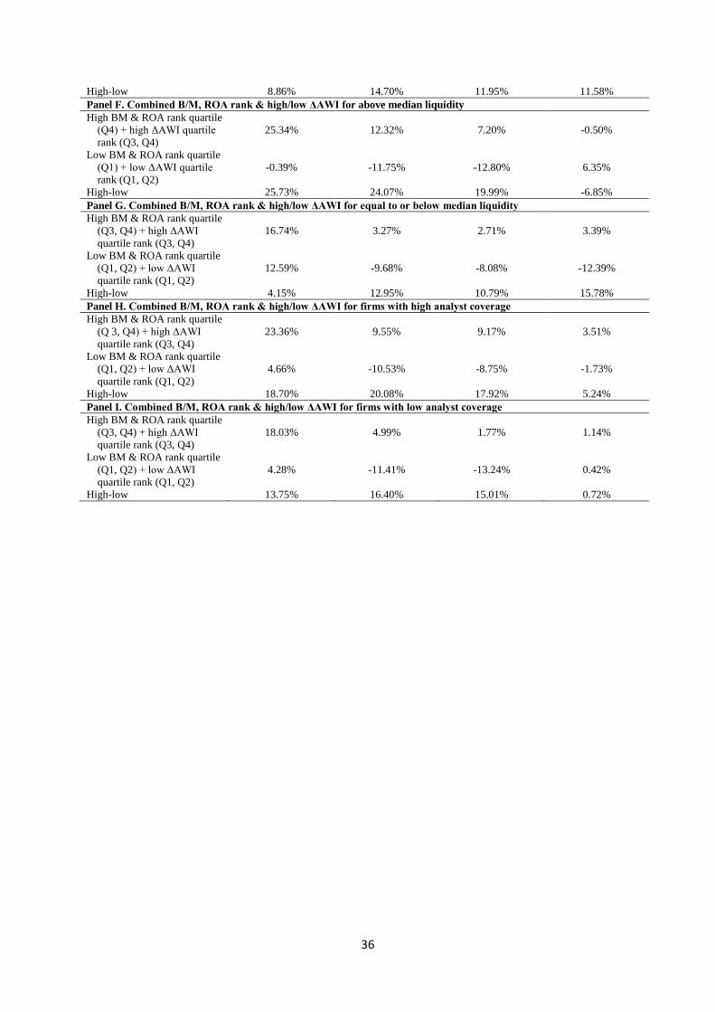
Panels F and G of Table 6 show that portfolio performance tends to be higher for stocks
with higher liquidity measured by high and low yearly share turnover (based on the median).
Panels H and I of Table 6 display portfolio performance based on the level of analyst coverage
(above or below median). The results show that the portfolio performance is not especially
sensitive to whether the number of analysts following the firm is high or low. Taken together, the
results in Table 6 indicate that portfolio performance is not significantly driven by size, liquidity
or analyst coverage, although performance is slightly higher for larger, more liquid and more
analyzed firms.21
4.3.3. The timing of the use of portfolio concentration data
The main specifications in Table 2 utilize portfolio concentration data for sorting in the
last phase after having made value and quality sorts. Alternatively, one could use portfolio
concentration data already in the first stage in which case the initial stock selection would be
21 Piotroski (2000) finds that value stocks that are smaller and associated with higher asymmetric information tend to
have higher returns in the US.
23
based on the combined ranks of ΔAWI and value (book-to-market) as well as on the combined
ranks of ΔAWI, value, and quality (ROA). Though not reported in a table, the results indicate
that the portfolio performance is higher when the portfolio holdings data is used in the last stage,
or put differently, not included in the initial stock selection. For example, a long-short portfolio
(high-low) using the combined ranks of ΔAWI, value, and ROA has lower performance than a
portfolio initially selected on value and quality with a final screening that includes stocks with
ΔAWI above the mean (Panel D, Table 2). Thus, the results indicate that holdings data should be
used to complement value and quality in the final stage.
4.3.4. Alternative timings of accounting data and stock returns, and stock return sub-periods
I also consider different lags when using historical accounting data. First, I consider
lagging the book value of equity (t-2) and Return on Assets one year (t-2), while using the
market value of equity from year-end (t-1). In the specifications with longer lags for accounting
data, I measure stock returns over the period Februaryt-Januaryt+1. As displayed in Panel A of
Appendix 2, the results are not very sensitive to how the book equity value or ROA are lagged.
The results using these lags are very similar to the main results.
Panels B-D of Appendix 2 show the returns for portfolios based on combined value and
quality ranks for high and low changes in portfolio concentration over the portfolio formation
sub periods 1997-2000, 2001-2003, and 2004-2006. For these sub-periods, the returns are
consistently higher for the high value, quality, and high change in portfolio concentration than
for the low portfolio. Although, there are variations in the return levels between the time periods,
the pattern for the difference between the high and low portfolios is rather consistent which gives
support to the conclusions regarding the results in Table 2 estimated for the full period.
24
5. Summary and conclusion
This paper explores whether information on investors’ equity portfolio concentration can
be beneficial to value investors. Using unique data on all the more than 1.3 million investor
portfolios in the Finnish stock market over a ten-year period, I find that data on changes in
average investor portfolio concentration in firms, a proxy for investor confidence, can be used to
improve the performance of value portfolios and portfolios based on combined value and quality
ranks. The results also indicate that the portfolio performance is somewhat higher when portfolio
concentration is calculated for larger, and presumably more informed, shareholders. In addition,
the results show that increases in ownership concentration can be used as an additional signal to
obtain improved portfolio performance of value oriented strategies, although the portfolio
concentration seems to be a better signal than ownership concentration. Overall, the results
indicate that it is possible to increase the performance of value-style portfolios by using data on
shareholders’ portfolio holdings without increasing portfolio risk. Future research could further
explore, for example, how investor characteristics and other corporate governance variables
could be incorporated into the fundamental analysis of firms.
25
References
Asness, C.S., A. Frazzini and L.H. Pedersen (2014), ‘Quality Minus Junk.’ SSRN working paper
(http://ssrn.com/abstract=2312432).
Bebchuk, L., A. Cohen and A. Ferrell (2009),’What Matters in Corporate Governance?’ Review
of Financial Studies, Vol. 22, pp. 783-827.
Carhart, M. (1997), ‘On Persistence in Mutual Fund Performance,’ Journal of Finance; Vol. 52,
pp. 57-82.
Dehning, B, T. Stratopoulos (2003), ‘Determinants of Sustainable Competitive Advantage due to
an IT-Enabled Strategy,’ Strategic Information Systems, Vol. 12, pp. 7-28.
Demsetz, H. (1986), ‘Corporate Control, Insider Trading, and Rates of Return,’ American
Economic Review, Vol., 76, pp. 313-316.
Dickinson, V., G.A. Sommers (2012), ‘Which Competitive Efforts Lead to Future Abnormal
Economic Rents? Using Accounting Ratios to Assess Competitive Advantage’, Journal
of Business Finance & Accounting, Vol. 39, pp. 360-398.
Edmans, A. (2009), ‘Blockholder Trading, Market Efficiency, and Managerial Myopia,’ Journal
of Finance, Vol. 64, pp. 2481-2511.
Edmans, A. (2014), ‘Blockholders and Corporate Governance’, Annual Review of Financial
Economics, Vol. 6, pp. 23-50.
Ekholm, A. and B. Maury (2014), ‘Portfolio Concentration and Firm Performance,’ Journal of
Financial and Quantitative Analysis, Vol. 49, pp. 903-931.
Fama, E.F. and K.R. French (1992), ‘The Cross-Section of Expected Stock Returns,’ Journal of
Finance, Vol. 47, pp. 427-465.
Fama, E.F. and K.R. French (1998), ‘Value versus Growth: The International Evidence,’ Journal
of Finance, Vol. 53, pp. 1975-1999.
Fidrmuc, J.P., M. Goergen and L. Renneboog (2006), ‘Insider Trading, News Releases, and
Ownership Concentration,’ Journal of Finance, Vol. 61, pp. 2931-2973.
26
Gompers, P., J. Ishii and A. Metrick (2003), ‘Corporate Governance and Equity Prices,’
Quarterly Journal of Economics, Vol. 118, pp. 107-156.
Gow, I., G. Ormazabal and D Taylor (2010), ‘Correcting for Cross-Sectional and Time-Series
Dependence in Accounting Research’, The Accounting Review, Vol. 85, pp. 483-512.
Grinblatt, M. and M. Keloharju (2000), ‘The Investment Behavior and Performance of Various
Investor Types: A Study of Finland's Unique Data Set,’ Journal of Financial Economics,
Vol. 55, pp. 43-67.
Hagstrom, R.G. (2005), The Warren Buffett Way. Second Edition. (New Jersey: Wiley & Sons).
Haugen, R.A. (1999), The Inefficient Stock Market: What Pays Off and Why. Second Edition.
Pearson Education. (USA: Upper Saddle River).
Haugen, R.A. and N.L. Baker (1996), ‘Commonality in the Determinants of Expected Stock
Returns,’ Journal of Financial Economics, Vol. 41, issue 3, pp. 401-439
Haugen, R.A. and N.L. Baker (2010), ‘Case Closed’, in: J.B. Guerard Jr., J.B. (eds), The
Handbook on Portfolio Construction: Contemporary Applications of Markowitz
Techniques (Springer), pp 601-619.
Ivkovic, Z., C. Sialm and S. Weisbenner (2008), ‘Portfolio Concentration and the Performance
of Individual Investors,’ Journal of Financial and Quantitative Analysis, Vol. 43, pp. 613-
656.
Jaffe, J.F. (1974), ‘Special Information and Insider Trading,’ Journal of Business, Vol. 47, pp.
410-428.
Jensen, M. (1968), ‘The Performance of Mutual Funds in the Period 1945–1964,’ Journal of
Finance, Vol. 23, pp. 389–416.
Kaperczyk, M.T. and A. Seru (2007), ‘Fund Manager Use of Public Information: New evidence
on Managerial Skills,’ Journal of Finance, Vol. 62, pp. 485-528.
Kallunki, J.-P., H. Nilsson and J. Hellström (2009), ‘Why do Insiders Trade? Evidence Based on
Unique Data on Swedish Insiders,’ Journal of Accounting and Economics, Vol. 48, pp.
37-53.
27
Lakonishok, J., A. Shleifer and R. Vishny (1994), ‘Contrarian Investment, Extrapolation and
Risk,’ Journal of Finance, Vol. 49, pp. 1541–1578.
La Porta, R., J. Lakonishok, A. Shleifer and R. Vishny (1997), ‘Good News for Value Stocks:
Further Evidence on Market Efficiency,’ Journal of Finance, Vol. 52, pp. 859–874.
Mohanram, P.S. (2005), ‘Separating Winners from Losers among Low Book-to-Market Stocks
Using Financial Statement Analysis,’ Review of Accounting Studies, Vol. 10, pp. 133-
170.
Novy-Marx, R. (2013), ‘The Other Side of Value: The Gross Profitability Premium,’ Journal of
Financial Economics, Vol. 108, pp. 1-28.
Novy-Marx, R. (2014), ‘Quality Investing,’ Working Paper, University of Rochester.
Petersen, M.A. (2009), ‘Estimating Standard Errors in Finance Panel Data Sets: Comparing
Approaches.’ Review of Financial Studies, Vol. 22, pp. 435-480.
Piotroski, J.D. (2000), ‘Value Investing: The Use of Historical Financial Statement Information
to Separate Winners from Losers,’ Journal of Accounting Research, Vol. 38 Supplement,
pp. 1-41.
Piotroski, J.D. and E.C. So (2012), ‘Identifying Expectation Errors in Value/glamour Strategies:
A Fundamental Analysis Approach,’ Review of Financial Studies, Vol. 25, pp. 2841-
2875.
28
Table 1. Descriptive Statistics
This table shows descriptive statistics for variables used in the study. The sample covers Finnish listed firms (excluding banks and insurance companies). Value portfolios are formed at the end of April in year t+1 during a ten-year period (1997-2006). Accounting and valuation variables are measured at end of year t-1 (1996-2005). The change in AWI (average weight index) for all, 0.1%, and 1% shareholders is measured from year-end t-2 to t-1, respectively. The change in HFI is the change in the Herfindahl index of all shareholdings in a firm from year-end t-2 to t-1. ROA is defined as earnings before interest and taxes (EBIT) divided by total assets in year t-1. Book-to-market is the book value of shareholders’ equity divided by the market capitalization of the firm’s shares in year-end t-1. Stock returns are measured over the period May year t to April year t+1 and defined in section 3.5. Analyst coverage is the number of analysts following a firm. F-score is the Piotroski (2000) measure of financial strength. Stdev returns is the standard deviation in daily stock returns during a year. Momentum is the 6 month stock return prior to portfolio formation. Trading volume is the trading volume for the year. Panel A includes all firms and Panel B includes firms in the highest book-to-market quarter each year. The number of observations varies due to data availability.
hold return, May-April) 0.1530 0.3584 -0.8384 1.6695 184
Market-adjusted returns (12 month buy and hold return, May-April)
0.0021 0.3720 -1.0666 1.1797 184
CAPM alpha (monthly data, May-April )
0.0013 0.0262 -0.1029 0.0836 184
Carhart four factor alpha (monthly data, May-April )
0.0020 0.0388 -0.1207 0.1451 184
30
Table 2. Investment Returns to Value, Quality, and Portfolio Concentration
This table shows the investment returns in percentage to value investing strategies using data on Finnish listed OMXH main list firms (excluding banks and insurance companies) over a ten-year period. Portfolios are formed in the end of April in year t each year (1997-2006). Accounting and valuation variables are measured at end of year t-1. The change in AWI (average weight index) is measured from year-end t-2 to t-1. Stock returns are measured over the period May year t to April year t+1 if not otherwise specified. Panel A shows returns for high book-to-market quartile (value) firms and low book-to-market quartile (glamour) firms. Panel B shows returns for high book-to-market and low book-to-market firms controlling for change in AWI. Panel C shows returns for high and low quartile portfolios formed based on the combined book-to-market and ROA rank. Panel D splits the portfolios in Panel C based on changes in AWI (above or below median change). Panel E shows returns for the combined book-to-market and ROA rank that are based on increases in AWI or decreases in AWI.
Strategy Description of Strategy
Raw return (12 month buy and
hold return, May-April)
Market-adjusted
returns (12 month buy and hold
return, May-April)
CAPM alpha (monthly data (x12), May-
April)
Carhart four factor alpha
(monthly data (x12), May-
April)
(1) (2) (3) (4) Panel A. Value stocks vs. glamour stocks Value High BM (Q4) 16.61% 0.61% 2.16% 2.16% Glamour Low BM (Q1) 9.09% -8.08% -8.66% 3.31% Value-Glamour Value-Glamour 7.53%** 8.69%** 10.81%*** -1.15% Panel B. Value stocks by high and low ΔAWI Concentrated Value High BM (Q4) & high
Positive ΔAWI - negative ΔAWI within high BM & ROA portfolio
6.87% 14.63%*** 7.08%* 12.56%**
*, **, and *** indicate statistical significance at the 10, 5, and 1 percent levels, respectively.
32
Table 3. Investment Returns to Value, Quality, and Portfolio Concentration Using Alternative Specifications of Portfolio Concentration
This table shows the investment returns in percentage to value investing strategies using data on Finnish listed OMXH main list firms (excluding banks and insurance companies) over a ten-year period. Portfolios are formed in the end of April in year t each year (1997-2006). Accounting and valuation variables are measured at end of year t-1. The change in AWI (average weight index) is measured from year-end t-2 to t-1. Stock returns are measured over the period May year t to April year t+1. Panel A shows returns for high and low quartile portfolios formed based on the combined book-to-market and ROA rank that are based on changes in AWI (above or below median change) using data on 0.1% shareholdings only. Panel B A shows returns for high and low quartile portfolios formed based on the combined book-to-market and ROA rank that are based on changes in AWI (above or below median change) using data on 1% shareholdings only. Panel C shows returns for the combined book-to-market and ROA rank portfolio for increases in HFI (Hefindahl index of all shareholdings) or decreases in HFI.
*, **, and *** indicate statistical significance at the 10, 5, and 1 percent levels, respectively.
Strategy Description of Strategy Raw return (12 month buy and
hold return, May-April)
Market-adjusted returns (12
month buy and hold return, May-April)
CAPM alpha (monthly data (x12), May-
April )
Carhart four factor alpha
(monthly data (x12), May-
April ) (1) (2) (3) (4) Panel A. Value, Quality & ΔAWI for 0.1% shareholders Profitable Value,
Concentration – Increased Own. Dispersion within Profitable Value
Positive ΔHFI - low ΔHFI within high BM & ROA portfolio 6.24% 5.82% 3.89% 4.83%
33
Table 4. Multivariate analysis
This table shows cross-sectional regressions of market-adjusted stock returns on book-to-market, ROA, size, momentum, and change in AWI. The sample consists of Finnish listed OMXH main list firms (excluding banks and insurance companies) over a ten-year period. The sample is restricted to value-oriented firms (book-to-market above median each year). Market-adjusted returns are measured over the period May year t to April year t+1. Accounting and valuation variables are measured at end of year t-1 (1996-2005). The change in AWI (average weight index) is measured from year-end t-2 to t-1 and is calculated for all (ΔAWI), 0.1% shareholders ΔAWI_0.1%, or 1% shareholders (ΔAWI_1%) depending on the model. Robust standard errors that control for firm and year clustering (Petersen , 2009) are in parentheses below the coefficient estimates.
*, **, and *** indicate statistical significance based on robust standard errors at the 10, 5, and 1 percent levels, respectively.
This table shows mean values of risk-related measures for various portfolios sorted based on information on value, quality, and portfolio concentration. The sample consists of Finnish listed OMXH main list firms (excluding banks and insurance companies) over a ten-year period. Portfolios are formed in the end of April in year t each year (1997-2006). The change in AWI (average weight index) is measured from year-end t-2 to t-1. Column 1 shows CAPM β for the portfolios. Column 2 shows standard deviations of past 5-year (t-5 - t-1) ROA for portfolios. Q4 is the highest quarter and Q1 is the lowest quarter each year, respectively. Panels A-D use data on all shareholders to calculate AWI in a firm, whereas Panel E uses data on at least 1% shareholdings to calculate AWI.
*, **, and *** indicate statistical significance at the 10, 5, and 1 percent levels, respectively.
Strategy Description CAPM β (systematic risk)
Standard deviation of 5-year ROA
(1) (2) Panel A. All shareholders Value High BM rank (Q4) 0.6001 3.9526 Glamour Low BM rank (Q1) 1.0379 7.9117 Value-Glamour High-Low -0.4378*** -3.9591*** Panel B. All shareholders Concentrated Value High BM rank (Q4) & high
Table 6. Investment Returns to Value, Quality, and Portfolio Concentration Using Alternative Data Partitions
This table shows the investment returns in percentage to value investing strategies using data on Finnish listed OMXH main list firms (excluding banks and insurance companies) over a ten-year period. Portfolios are formed in the end of April in year t each year (1997-2006). Accounting and valuation variables are measured at end of year t-1. The change in AWI (average weight index) is measured from year-end t-2 to t-1. Stock returns are measured over the period May year t to April year t+1. Panel A shows the returns to portfolios ranked by value and F-score with and without ΔAWI screens. Panel B shows returns for high book-to-market and low book-to-market firms controlling for change in AWI. Panel C shows returns for high and low quartile portfolios formed based on the combined book-to-market and ROA rank. Panels D and E split the portfolios in Panel D based on market value of equity (MVE) (above or below median MVE). Panels F and G split the portfolios in Panel D based on liquidity (share turnover in euro) (above or below median share turnover). Panels H and I split the portfolios in Panel D based on analyst coverage (above or below median number of analysts following the firm).
Raw return (12 month buy and hold return, May-April)
Market-adjusted returns (12 month
buy and hold return, May-April)
CAPM alpha (monthly data (x12),
May-April)
Carhart four factor alpha (monthly data (x12), May-April)
(1) (2) (3) (4) Panel A. Combined value and F-score rank High BM & F-score rank
quartile (Q4) 19.97% 1.63% 0.17% -0.18%
Low BM & F-score rank quartile (Q1)
14.49% -2.35% -0.16% 0.10%
High-Low 5.47% 3.98% 0.33% -0.29% High BM & F-score rank
High-Low 9.10% 11.60% 12.09% -0.66% Panel C. Above median BM & ROA rank stocks vs. equal to or below median BM & ROA rank firms by high and low ΔAWI High BM & ROA rank
High-low 25.73% 24.07% 19.99% -6.85% Panel G. Combined B/M, ROA rank & high/low ΔAWI for equal to or below median liquidity High BM & ROA rank quartile
This table shows spearman correlations for main variables used in the study. The sample covers Finnish listed firms (excluding banks and insurance companies). Accounting and valuation variables are measured at end of year t-1 (1996-2005). The change in AWI (average weight index) for all, 0.1%, and 1% shareholders is measured from year-end t-2 to t-1, respectively. The change in HFI is the change in the Herfindahl index of all shareholdings in a firm from year-end t-2 to t-1. ROA is defined as earnings before interest and taxes (EBIT) divided by total assets in year t-1. Book-to-market is the book value of shareholders’ equity divided by the market capitalization of the firm’s shares in year-end t-1. Stock returns are measured over the period May year t to April year t+1 (see Section 3.5 for details). Other variables are defined in Table 1. Panel A includes all firms and Panel B includes firms in the highest book-to-market quarter each year. The number of observations varies due to data availability.
Appendix 2. Investment Returns to Value, Quality, and Portfolio Concentration (%) Using Alternative Timings of Variables
This table shows the investment returns in percentage to value investing strategies using data on Finnish listed OMXH main list firms (excluding banks and insurance companies). Portfolios are formed at the end of April in year t+1 during a ten-year period (1997-2006). Accounting and valuation variables are measured at end of year t-1 (1996-2005). The change in AWI (average weight index) is measured from year-end t-2 to t-1. Stock returns are measured over the period May year t to April year t+1 if not otherwise specified. Panel A shows returns for high/low quartile portfolios formed based on combined ranks for book-to-market, ROA, and change in AWI using lagged accounting data (t-2) with returns measured for February t to January t+1. Panels B through D show returns for high/low quartile portfolios formed based on combined ranks for book-to-market, ROA, and ΔAWI for the sub periods 1997-2000, 2001-2003, and 2004-2006.
Raw return (12 month buy and hold return, May-April)
Market-adjusted returns (12 month
buy and hold return, May-April)
CAPM alpha (monthly data (x12),
May-April )
Carhart four factor alpha (monthly data (x12), May-April )
(1) (2) (3) (4) Panel A. Combined B/M, ROA rank & high/low ΔAWI, lagged accounting data t-2, returns Feb t - Jan t+1 High BM & ROA rank quartile