Valuing Alternative Work Arrangements∗

Alexandre Mas

Princeton University and NBER

Amanda Pallais

Harvard University and NBER

March 2017

Abstract

We employ a discrete choice experiment in the employment process for a national call center to

estimate the willingness to pay distribution for alternative work arrangements relative to traditional office

positions. Most workers are not willing to pay for scheduling flexibility, though a tail of workers with

high valuations allows for sizable compensating differentials. The average worker is willing to give up

20% of wages to avoid a schedule set by an employer on short notice, and 8% for the option to work from

home. We also document that many jobseekers are inattentive, and we account for this in estimation.

∗We would like to thank Jason Abaluck, Joshua Angrist, David Autor, David Card, Henry Farber, Edward Freeland, ClaudiaGoldin, Nathan Hendren, Lawrence Katz, Patrick Kline, Alan Krueger, Claudia Olivetti, Jesse Shapiro, Basit Zafar, and seminarparticipants at the Advances with Field Experiments conference, Brown University, CEMFI, CEPR/IZA Annual Labour EconomicsSymposium, Executive Office of the President of the United States, Harvard University, MIT, NBER Summer Institute, StanfordUniversity, Tufts University, UC Berkeley, University of Chicago, University College London, Universitat Pompeu Fabra, Uni-versity of Tel Aviv, Wellesley College, Wharton, and the University of Zurich for their many helpful comments and suggestions.We would also like to thank Jenna Anders, Stephanie Cheng, Kevin DeLuca, Jason Goldrosen, Disa Hynsjo, and Carl Liebermanfor outstanding research assistance. Financial support from NSF CAREER Grant No. 1454476 is gratefully acknowledged. Theproject described in this paper relies on data from a survey administered by the Understanding America Study, which is main-tained by the Center for Economic and Social Research (CESR) at the University of Southern California. The content of thispaper is solely the responsibility of the authors and does not necessarily represent the official views of USC or UAS. This projectreceived IRB approval from Princeton (#0000006906) and Harvard (#15-0673). This study can be found in the AEA RCT Registry(AEARCTR-0001250).

1 Introduction

Alternative work arrangements, such as flexible scheduling, working from home, and part-time work are a

common and by some measures a growing feature of the U.S. labor market.1 While these arrangements may

facilitate work-life balance, they are not necessarily worker-friendly. Many jobs have irregular schedules,

whereby workers cannot anticipate their work schedule from one week to the next; many workers are on-call

or work during evenings, nights, and weekends. The emergent gig economy, while still small (Ferrell and

Greig, 2016), has put these trade-offs into focus. Workplace flexibility has been touted as both one of the

benefits and costs of the fragmentation (or “Uberization”) of the workplace.2

There is a policy debate as to whether and how government should encourage alternative work ar-

rangements that promote work-life balance (Council of Economic Advisors, 2010). This debate extends

to regulation of overtime in the Fair Labor Standards Act, flexibility options in the Family Medical Leave

Act, and initiatives to promote telecommuting. Scheduling policy is a key decision for employers. There

is a well-established belief among human resource consultants that workplace flexibility policies (broadly

defined) help attract and retain employees.3 Recently, prominent companies have announced moves away

from irregular scheduling. In 2016, Walmart shifted from giving managers discretion on shift scheduling to

offering some workers predictable fixed shifts and the ability to make their own schedules (DePillis, 2016).

Starbucks announced that it was revising its policies to end irregular schedules to promote “stability and

consistency” in scheduling (Kantor, 2014). These changes came during increasing legal scrutiny of irregular

scheduling work practices (Weber, 2015).

Despite this active debate on how alternative work arrangements should be promoted and regulated,

very little is known about how workers actually value different arrangements. Efficient public and corporate

policies on alternative work arrangements require an understanding of these valuations. One approach is

estimating compensating wage differentials on workplace amenities, building on the theoretical framework

for hedonic pricing in Rosen (1974) and Rosen (1986). An enormous literature has sought to do this using

cross-sectional and longitudinal data, but it is well known that estimates from these approaches are unstable

to adding person or workplace controls, and are often wrong-signed.4 This fragility of compensating differ-

entials estimates may be due to the presence of unmeasured worker and firm characteristics, measurement1Katz and Krueger (2016) document a significant rise in alternative work arrangements between 2005 and 2015. They consider

temporary help agency workers, on-call workers, contract company workers, and independent contractors or freelancers as workerswith alternative arrangements.

2For examples, see “Uber’s Business Model Could Change Your Work,” New York Times, January 28, 2015.3See, for example, Deloitte (2013).4Papers in this literature include those that estimate the value of statistical life, summarized in Viscusi and Aldy (2003) and stud-

ies reviewed in Smith (1979), Brown (1980), Goddeeris (1988), Lanfranchi et al. (2002), Kostiuk (1990), and Oettinger (2011). Halland Mueller (2015), Sorkin (2015), and Taber and Vejlin (2016) use worker flows to infer the importance of non-wage amenities.

1

error, or the presence of search frictions in the labor market (Hwang et al., 1998; Lang and Majumdar, 2004;

Bonhomme and Jolivet, 2009). Additionally, in standard models of equalizing differences, such as Rosen

(1986), compensating wage differentials are set to equate the utility of marginal workers in jobs with and

without an amenity, providing only limited information on valuations for other workers.

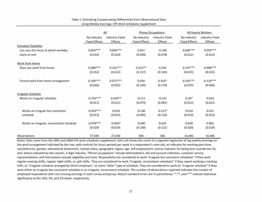
Table 1 shows the difficulty of estimating compensating differentials for the work arrangements we

study. Using data from the CPS Work Schedules Supplement, we regress weekly wages separately on indi-

cators for having a given work arrangement. We control for a variety of worker (and some job) characteris-

tics. Throughout, more pleasant work arrangements are correlated with higher wages. For example, workers

who have control over when they start and end work earn 6% more than workers who do not, while workers

who have formal work-from-home arrangements earn about 10% more.5 On the other hand, workers with

irregular schedules that change from week to week earn about 8% lower wages.

In this paper we report estimates of worker valuations over alternative work arrangements from a field

experiment with national scope. The experiment elicits preferences on work arrangements by building

a simple discrete choice experiment into the application process for a national call center. In this way we

employ a method that can flexibly back out a willingness to pay (WTP) distribution from close to real market

transactions.6 We consider a number of commonly-discussed arrangements, including flexible scheduling,

working from home, and irregular schedules.

We carried out a large-scale recruitment drive to staff a national call center. The purpose of the call

center was to implement telephone surveys, unrelated to this project. We posted job ads on a major elec-

tronic job board in 68 metro areas for telephone interviewer positions. The ads described the position and

several required qualifications, but did not include any additional information about the nature of the job

such as the schedule or whether the job was on-site. During the application process, we asked applicants

their preference between two positions: a baseline position offering a traditional 40 hour 9 am – 5 pm

Monday-Friday on-site work arrangement (in the applicant’s local area) and a randomly-chosen alternative

arrangement. The alternatives included flexible scheduling, working from home, and positions that gave the

5Garriety and Shaffer (2001 and 2007) similarly find that both flextime and working from home are associated with higherwages using data from the CPS Work Schedules Supplement.

6Discrete choice experiments are an extension of the contingent valuation literature whereby rather than directly asking peoplefor valuations over an attribute (the stated preference method), people are given the choice of two or more scenarios and are askedto choose their preferred option. These scenarios usually vary the attributes and the prices and WTP can be estimated using randomutility models (McFadden, 1973; Manski, 1977). Choice experiments have been shown to have better properties relative to statedpreference valuation methods (Hanley et al., 1998). A question is whether these experiments, which are usually survey-based,correspond to actual market behavior. This is something we can overcome by embedding the choice in a real market setting.Diamond and Hausman (1994), who critique stated preference valuation methods, hypothesize that the problem with the approachis not methodological but due to “an absence of preferences” over the attributes they are being asked to value. This is far less of aconcern here since we are asking people to make choices over realistic work arrangements.

2

employer discretion over scheduling. We also randomly varied the wage difference between these two op-

tions. In the experimental portion of the application we were silent on whether these were actual positions;

we simply asked applicants to tell us their preference over two job descriptions. This gave us latitude to

vary the parameters of the position descriptions. However, the positions were fully consistent with the type

of job we advertised thereby approximating a market choice.7 We elicited preferences from approximately

7,000 applicants, allowing us to estimate the WTP distribution for a number of common alternative work

arrangements using a simple discrete choice framework.8

There are several challenges to the approach that require addressing. First, prior to running the experi-

ment we hypothesized that some applicants would not pay close attention to the position descriptions. We

implemented several placebo tests which confirmed that approximately 25% of applicants are inattentive. By

estimating the inattention rate, we can account for misclassification in the econometric model and recover

the unbiased WTP distribution.9

Second, we elicit preferences only from jobseekers who respond to this position, and thus our WTP

estimates are directly relevant only for this group. However, several analyses instill confidence that these

estimates may be applicable to a wider slice of the population. First, we show that work arrangements in

this occupation are similar to those in the economy more generally, so that these applicants are not neces-

sarily selected based on their value for workplace flexibility. Second, weighting the estimates by observed

worker characteristics to match a nationally-representative sample of workers does not change our estimates

substantially. Finally, we designed a module in the nationally-representative Understanding America Study

(UAS) that elicited preferences over scheduling flexibility, working from home, and employer discretion

using a choice framework similar to the one described above. Valuations from the survey are very similar

to our experimental results. This result is noteworthy by itself in that it shows that survey-based choice

experiments with vignettes, when designed properly, elicit responses that are close to market choices. The

survey has additional advantages that it has information on worker characteristics that are not possible to

obtain from applicants, such as the presence of children, and that there is no potential for responses to the

survey to act as a signal to potential employers.

Our first, surprising, finding is that the great majority of workers do not value scheduling flexibility:

either the ability to set their own days and times of work at a fixed number of hours, or the ability to choose

7The actual jobs combined the highest wage the applicant viewed, scheduling flexibility, and the ability to work remotely.8The applicant figure refers to the number of jobseekers who initiated the application process and chose one of the two jobs

presented. Of these, 77% completed the application and applied for the job. At present, we have contacted 150 applicants to offerthem jobs, subject to their passing a required criminal background check.

9It is an interesting question whether this type of inattention should be taken into account when estimating the WTP for thesepositions. This type of inattention may represent a real friction in the labor market. By adjusting the estimates our frameworkallows us to estimate the welfare costs of inattention.

3

the number of hours they work. This is true both among job applicants and survey respondents in the

UAS. While the average WTP for jobs with flexible schedules is low, there is a long right tail in the WTP

distribution for these arrangements, reflecting people who are relatively inelastic to the price of flexibility.

Thus, there remains considerable potential for reasonably large market compensating wage differentials for

flexible scheduling. We find evidence of heterogeneity in valuations in all of the job attributes we consider;

mean WTP estimates may differ substantially from marginal WTP estimates. Caution is therefore warranted

when interpreting cost-benefit analyses that are based on average valuations alone.

One reason workers do not value flexibility in the number of hours they work is that most want to work

40 hours per week. When given a choice between a 20 hour-per-week job and a 40 hour-per-week job,

the average worker was willing to take a $6 per hour pay cut for the 40-hour position. Most workers also

require a wage premium to work overtime. When given a choice between a 50-hour job in which the last

10 hours were paid at time-and-a-half and a 40-hour job paying the same base wage, 55% chose the 50

hour-per-week job. The Fair Labor Standards Act’s overtime requirements – which make employers pay

most hourly workers 1.5 times wages for hours over 40 hours per week – makes the average worker close to

indifferent to working overtime in our setting.

Second, of the employee-friendly alternatives we consider, working from home is the most valued. On

average, job applicants are willing to take 8% lower wages for the option of working from home. The fact

that working from home is still relatively uncommon – even in the industry in which we are hiring – while

there is a substantial share of workers willing to take wage cuts for these jobs, suggests that it may be costly

for employers to offer this arrangement. Taking our estimates of the WTP distribution at face value, the

share of hourly workers with work-from-home arrangements (10%) implies that it would cost at least 21%

of wages for employers to switch to work-at-home positions.

Third, job applicants and UAS respondents have a strong aversion to jobs that permit employer discretion

in scheduling: the average applicant is willing to take a 20% wage cut to avoid these jobs, and almost 40% of

applicants would not take this job even if it paid 25% more than a M-F 9 am - 5 pm position. The distaste for

jobs with employer discretion is due to aversion to working non-standard hours, rather than unpredictability

in scheduling. For most workers, a traditional M-F 9 am - 5 pm schedule works well: workers are not willing

to take lower wages to set their schedules on top of this, but they are willing to take substantial wage cuts to

avoid evening and weekend work.

The paper also contributes to our understanding of how men and women differentially value workplace

amenities and how this translates into the observed gender wage gap. A large literature has examined gender

4

differences in work arrangements and asked to what extent these differences can explain gender wage gaps.10

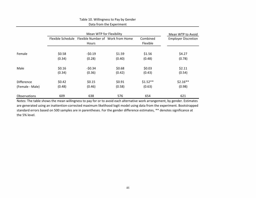
We find that women are more likely to select flexible work arrangements than are men. While, on average,

women do not tend to value flexible schedules, they do place a higher value on working from home and

avoiding irregular work schedules than do men. This is particularly true for women with young children.

Despite this, women are only slightly more likely to be in work-from-home jobs and slightly less likely to be

in jobs with irregular schedules. The differences in observed work arrangements are not large enough to lead

to significant gender gaps even with substantial compensating wage differentials. While there are gender

differences in the propensity to select into alternative work arrangements, there is no detectable relationship

between workers’ education or score on a cognitive test we administered and their choices.

Relative to the previous literature, our study is closely related to Eriksson and Kristensen (2014) and

Wiswall and Zafar (2016). Eriksson and Kristensen (2014) use a vignette method to elicit WTP for various

job amenities and fringe benefits in an internet sample of Dutch respondents. One of the amenities they

consider is scheduling flexibility. Our UAS survey module also uses use a vignette method to elicit pref-

erences for flexibility and other arrangements. Wiswall and Zafar (2016) use a stated preference approach

to understand how a sample of undergraduate students values job characteristics in hypothetical future jobs,

including the availability of part-time work, which is one measure of work flexibility. The advantage of

these approaches is that they provide considerable scope for quantifying a large range of job characteristics

and, in the Eriksson and Kristensen (2014) case, in a sample that is close to representative of the population

in which they are interested. The disadvantage to the approach is that it is unclear to what extent responses

to hypothetical questions are accurate and approximate behavior in a market setting. This concern has led to

a large literature probing hypothetical bias in the context of contingent valuation surveys (see e.g., List and

Shogren, 1998).

In terms of our field methodology, our approach is related to Flory et al. (2015), Hedegaard and Tyran

(2014), and Stern (2004). Flory et al. (2015) and Hedegaard and Tyran (2014) use data collected in the

application phase of a real job to learn about job seekers’ preferences. Flory et al. (2015) randomize job

applicants into different compensation packages and measure gender differences in the probability of apply-

ing as a function of the compensation scheme presented. This approach is informative about the direction

of preferences, but does not yield WTP measures. Hedegaard and Tyran (2014) focus on preferences about

co-workers’ ethnic backgrounds. In a novel approach to estimating market compensating differentials, Stern

(2004) uses multiple job offers for PhD job candidates in biology to estimate the tradeoff between starting

10Studies include Filer (1985), Goldin and Katz (2011), Goldin (2014), Flory et al. (2015), Goldin and Katz (2016), and Wiswalland Zafar (2016).

5

pay and the opportunity to conduct research. Our paper estimates preferences both in the field and via the

vignette method to get both the benefits of the flexibility and external validity of the vignette method and

the more realistic environment from the natural field experiment.

We begin by discussing our experimental design (Section 2) and conceptual and econometric framework

(Section 3). From there, we present our main estimates of workers’ valuations for alternative work arrange-

ments (Section 4) and show external validity through the nationally-representative UAS (Section 5). We

examine heterogeneity of WTP by subgroup in Section 6 and discuss the implications of our findings for

compensating differentials in Section 7.

2 Experimental Design

Our experiment is structured around the hiring process for a national call center that we staffed to implement

a labor market survey, unrelated to this project, during calendar year 2016. The experiment takes place

during the application process for these positions.

We posted advertisements for telephone interviewer positions on a national U.S. job search platform.

The platform has separate portals for most regions and we posted a customized ad in 68 large metro areas.

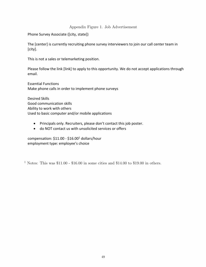
The ads were modeled off of existing ads on the site; the text of these ads is presented in Appendix Figure

1. They mentioned the necessary skills for the job, emphasized that the position did not include sales or

telemarketing, and included information about the job’s wage range.11 We provided no information about

the job’s schedule, location, or duration. The ad had a link to our website where interested jobseekers could

apply for a position.

We ran the labor market survey and conducted all hiring under the auspices of a center responsible for

the hiring. We did not disguise the center’s mission (the study of labor markets) or its personnel. However,

the center did not specify an affiliation with any university or this particular project. The center website is

professionally designed, and the feedback we received from applicants we spoke to is that the ad and the

website looked like those of a regular employer.

Once applicants followed the link to our site, they could apply by creating an account which required

them to enter their contact information, year of birth, and zip code. The next step in the application was a

voluntary self-identification page where applicants could provide their race/ethnicity and gender. The page

11The necessary skills specified were “good communication skills,” “ability to work with others,” and “used to basic computerand/or mobile applications.” The platform has a field for the compensation range. We filled this in to be consistent with the site’stypical practices as well as to encourage applications from interested participants and prevent applicants uninterested in jobs at thesewages from wasting their time. The wage range corresponded to the lowest and highest wage in the discrete choice experiment. Wehired at the highest wage in the range.

6

prominently stated that this information was optional and that the questions could be skipped, though the

vast majority of applicants responded.12 We did not feel that it would be appropriate to ask about marital or

parental status.

The third step of the application was the discrete choice experiment. Applicants were shown two de-

scriptions of job positions. The two positions differed in their characteristics (e.g., schedule or the ability

to work from home) and their hourly wages. The characteristics and wages were assigned to applicants

at random. While we could have shown each applicant multiple job descriptions with varying wages and

amenities, to minimize cognitive load, we limited the comparison to two options, a baseline and an alterna-

tive. In fact, we show that even with just two simple choices there is a substantial amount of inattention that

we have to account for. Additionally, in our judgment, more than two choices would have made the research

intent of this section too obvious. Implementing a between-subject design also allows us to avoid carry-over

effects. In Subsection 2.1 we describe the positions and randomization in more detail.

We told applicants that the type of work in both jobs was the same and asked them which job they would

choose if both were available. We assured applicants that we would not look at their choices before making

hiring decisions.13 The position descriptions were crafted to match the general description of the telephone

interviewer position advertised, but we did not tell applicants that these were the actual positions available.

Without specifying them, we indicated that there were other positions they could be hired for (“...regardless

of your choice you will be considered for all open positions”). This approach allowed us to use position

descriptions that deviated from the real jobs, while maximizing realism by describing positions that were

like the ones advertised.14

This step of the application process produces the key data for our analysis. The remainder of the ap-

plication asked about applicants’ background, including their educational attainment. We asked workers

six quantitative questions from the ACT WorkKeys, ranging from simple multiplication to basic algebra,

which we use as a measure of cognitive ability. Most (77%) workers who made a job choice completed the

application. Our main analysis uses all choices made, but we show in an appendix table that the results are

12Ninety-five percent of applicants provided their gender and 93% provided their race.13A potential concern is that applicants might not have believed us and disguised their desire for amenities to be more appealing

applicants. In Section 5 we discuss why we do not think this is the case. First, workers reported similarly low valuations forflexibility in a survey which had no effect on their employment outcomes. Second, applicants’ willingness to avoid the employerdiscretion job suggests they were not simply making the choice employers would find most appealing.

14The real job offered workers the maximum of the hourly wages shown in the position descriptions, plus additional compensationfor using their own phones and devices, flexible schedules (within the constraint of work hours being appropriate times to conducttelephone surveys), and remote work. The duration of the job was either one or two months and either 20 or 40 hours per week,depending on when they applied and the surveys we were running. This information was conveyed to all applicants who wereselected for the position at the time the job offer was first extended. At this time, we have contacted 150 applicants to offer themjobs, subject to their passing a required criminal background check.

7

similar if we restrict attention to workers who ultimately applied for the jobs.

2.1 Job Description and Wages

As described above, applicants were shown two position descriptions that differed in their work arrange-

ments and wages. In all of the main comparisons we use the same baseline job description: a traditional

40 hour-per-week, Monday - Friday 9 am - 5 pm position physically located near downtown of the city we

advertised in. This job description reads:

“The position is 40 hours per week. ¶ This is a M-F 9 am - 5 pm position. The work is exclusively on-site in

downtown [city]. This position pays [wage] dollars per hour.”

Here [city] is the city of the job ad (sometimes we used “center city” or a variant of this instead of “down-

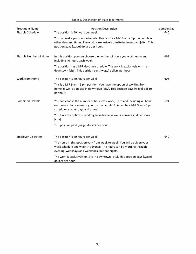
town” to conform to local terminology), and [wage] is a randomly-selected wage.15 We compare this base-

line position to five alternatives: (1) “flexible schedule:” a 40 hour-per-week position that allows the worker

to make his or her own work schedule, (2) “flexible number of hours:” a position that gives the worker the

choice of how many hours to work per week up to 40, (3) “work from home:” a 40 hour-per-week M-F 9

am - 5 pm position that gives the worker the option of working at home, (4) “combined flexible:” a position

that allows workers to make their own schedule, choose the number of hours they work, and work from

home, and (5) “employer discretion:” a 40 hour-per-week position that lets the employer select the worker’s

schedule (including weekends and evenings) with one week’s notice. The exact wording of each of the

descriptions is listed in Table 2.

We randomize which jobs workers are presented with and the wages in these jobs. For each metro area,

we randomly selected a maximum hourly wage of $16 or $19. In a given metro area, all applicants observed

one position that offered this maximum hourly wage.16 For the second option, we displayed a wage that was

a randomly-selected increment lower than the maximum wage. The increments – $0, $0.25, $0.50, $0.75,

$1.00, $1.25, $1.50, $1.75, $2.00, $2.25, $2.50, $2.75, $3.00, $4.00, and $5.00 – were selected to allow us

to capture both very small and very large WTP. Each increment had a uniform probability of selection. The

baseline position was sometimes (randomly) assigned the higher wage and sometimes assigned the lower

wage, so that we have approximate symmetry in the relative wages offered between the two positions. We

also randomized which job was presented first.

15The ¶ indicates a line break.16We select whether a city has a maximum wage of $16 or $19 at random.

8

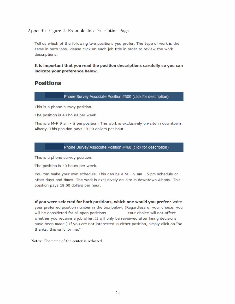
Appendix Figure 2 provides an example of the page with the job descriptions. This page was designed

with several goals in mind. First, we wanted to ensure that only the parameters of job would affect workers’

choice. Thus, we referred to jobs by number (not name) to minimize the extent to which job titles would

affect workers’ choices.17 We also made the wording of the job descriptions as similar as possible. To max-

imize the fraction of applicants who read both job applications carefully, we forced applicants to physically

click on each position to see the job description. We also required applicants to manually type the number

of the job they preferred to lessen the tendency to simply click through to the next page.

2.2 Measuring Inattention

A challenge for any experiment that manipulates information is accounting for the presence of people who

do not fully process the information. There is evidence in many contexts that agents are prone to inattention

(DellaVigna, 2009). Most of the available evidence on inattention involves consumers (e.g., Chetty et al.,

2009), and it has been shown that inattention can lead to significant optimization errors (Abaluck and Gruber,

2011). Given this evidence, we hypothesized that inattention might also be a feature of the labor market and

implemented a number of mechanisms to measure the inattention rate. We find direct evidence of such

frictions in our experiment.

First, we presented some applicants with two positions that were identical except that one of them stated

at the end, “This position is currently unavailable, please select the other position.”18 The fraction of workers

who choose the unavailable position is an indicator of the fraction of inattentive workers. Second, on the

page after the job choice, we asked workers whether the position they selected had “a fixed M-F, 9 am

to 5 pm schedule” or whether the position they selected had “an alternative schedule”.19 The fraction of

workers answering incorrectly (i.e., responding that they chose a fixed M-F 9 am - 5 pm schedule when

they chose an alternative schedule or vice versa) is another inattention measure. Finally, the measure we

utilize in the estimation approach, which is described in more detail in the next section, is the estimated

share of applicants who choose a dominated position when this position paid $5 per hour less than the

alternative. This approach is attractive because it allows us to calculate inattention rates that are specific

to each comparison and demographic group. We estimate that, on average, 14.5% of individuals chose the

dominated position when it paid $5 less than the alternative. In comparison, 13.3% of individuals answered

17These numbers were randomly assigned to jobs. The numbers were also balanced within comparisons, so if some individualswere given a choice between Position #78 which was inflexible and Position #81 which was flexible, other participants were facedwith a choice between Position #81 which was inflexible and Position #78 which was flexible.

18Both positions used the language from the baseline position.19We did not specify what the alternative schedule might be; workers in all of our main treatments saw the same wording of this

question.

9

which position they chose incorrectly and 13.0% chose the “unavailable” position. If inattentive applicants

made their choices randomly, the estimates imply that just over a quarter of the applicants were inattentive.

Because estimates of quantiles and higher order moments of the WTP distribution will be influenced by

inattention, we explicitly incorporate inattention into the maximum likelihood estimator.20 The methodology

is similar to those in studies that incorporate external measures of the misclassification of binary variables,

such as Card (1996). It has long been recognized in the literature on contingent valuation and discrete

choice experiments that inattention is a cause for concern (Johnson et al., 2013). However, we are unaware

of studies in this literature that explicitly incorporate inattention error rates into the econometric models to

estimate the WTP distribution. This may be due to the fact that most studies in this literature are focused

on mean valuations, where misclassification will lead to relatively little bias. Our findings highlight the

importance of accounting for inattention in even simple discrete choice experiments, particularly when the

analyst is interested in higher moments of the distribution.

3 Conceptual and Econometric Framework

In this section, we describe the econometric framework that we use to estimate the distribution of willingness

to pay for alternative work arrangements in Section 4. We use workers’ choices over positions to estimate

these distributions.

Building on Rosen (1986), we assume that an individual chooses between two jobs which are equivalent

except for the presence of an amenity (e.g., the ability to work from home, a traditional schedule) and the

wage. Our experimental design fits this framework by limiting the differences between the positions to these

two characteristics. Job A = 1 has the amenity, while job A = 0 does not. The difference in wages between

the two jobs is 4w = w1−w0. In the experiments 4w ∈ [−5,5]. Each individual i has a willingness to

pay WT Pi for the amenity: µ is the population mean willingness to pay, while σ is the population standard

deviation. If the individual is fully attentive, she prefers the job with the amenity if her willingness to pay

for the amenity (WT Pi) exceeds the price of the amenity −4w:

P4w ≡ Pr(WT Pi >−4w).

Inattentive individuals are equally likely to select either job. If 2α of individuals are inattentive, in

expectation half of them (α) will choose the dominated option by chance. Therefore, the probability that an

20We show in appendix tables that our results are robust to using any of the alternative methods of measuring the inattention rate.

10

individual chooses the job with the amenity is:

Pr(Ai = 1|4w) = P4w(1−α)+(1−P4w)α = F(b4w+ c; µ,σ)(1−2α)+α. (1)

Equation 1 is a mixture model that can be estimated by maximum likelihood (ML) given a parametric

assumption about the cdf of WT Pi : F(). We assume WT Pi follows a logistic distribution, though a

normality assumption works just as well. Under the logistic assumption, with estimates of b and c we can

fully characterize the WTP distribution: µ =−1∗ c/b and σ = 1/0.55b.21 The qth quantile of the WTP

distribution can be computed by inverting the cdf: 4wq = F−1(q; µ, σ). Standard errors are

bootstrapped.22

While the parameter α is identified in equation 1, we use our knowledge of which position is dominated

to first estimate this value, and then to fix this estimated value before estimating the maximum likelihood

model. Specifically, our estimate of α is the share of applicants who chose the dominated position (the

position without the amenity) when it paid $5 less per hour, that is, α = 1− E[Y |4w=5]. (We assume that

no attentive applicants choose the dominated position.) We estimate E[Y |4w=5] by estimating the linear

regression Y4w = γ +β4w+ζ4w for values of4w ranging from 2 to 5 and calculating α = 1−(

γ +5β

).

We estimate α separately by treatment- and (when applicable) subgroup. We present estimates without

the inattention correction as well. In practice, this correction will affect estimates at the tails of the WTP

distribution, but not estimates of the mean or median.23

An advantage of our design is that we can plot our estimates of P4w nonparametrically to assess distri-

butional assumptions. For a given4w, the share of individuals in the sample who choose A = 1 is:

Y4w = P4w(1−2α)+α + ε4w,

where ε4w represents sampling error. We use an estimate of α to transform this share so that it is an

unbiased estimate of the share of jobseekers whose willingness to pay for a job attribute exceeds −4w:

Y4w ≡Y4w− α

1−2α= P4w + ε4w.

We plot Y4w against4w to visually assess fit.

21The 0.55 parameter in the denominator corrects for the scale parameter.22We bootstrap standard errors to take into account variability in the estimation of the inattention rate.23We have also estimated WTP allowing α to be estimated internally within the model, as in Hausman et al. (1998). The resulting

WTP estimates are presented in an appendix table and very close to those from the approach that uses the dominated choice.

11

For most treatments the logistic specification provides a good description of the data, but in some cases

we can observe that the symmetry assumption seems to be violated. In particular, the logistic cdf does

not capture the extreme non-linearity in Y at 4w = 0 we observe for some comparisons. In these cases

E[Y | 4w

]is approximately 1 for most positive values of 4w and shifts downward close to 4w = 0. This

close-to-discontinuous shift suggests that there may be mass points in the cdfs of WTP that the logistic

distribution cannot accommodate. To account for this, we estimate a “breakpoint” model that nests a mass

point:

E[Y | 4w

]=

1, if4w > w∗

F(b4wi + c; µ,σ)(1−2α)+α, if4w≤ w∗,

where w∗ is a breakpoint. We impose the constraint b≤ 0 to ensure that predicted values can be interpreted

as a cdf. Rather than assume a value of w∗, we estimate a structural break model where we vary w∗ from

w∗ =−2 through w∗ = 5 (the no mass point case) and select the value of w∗ that minimizes the root mean

square error of the model.

To calculate the mean and variance of WTP in the breakpoint model we use the integration by parts

expression for computing a mean and variance of a distribution from a cdf:

µ =

0ˆ

−∞

(1− ˆY

)d4w−

∞

0

ˆY d4w

σ2 = 2

∞

0

4w(

1− ˆY)

d4w−2

0ˆ

−∞

4w ˆY d4w− µ2

The integrals are computed numerically, the quantiles are calculated by inverting the cdf, and the standard

errors are bootstrapped.

4 Willingness to Pay for Alternative Work Arrangements

4.1 Descriptive Statistics and Randomization Assessment

Our experimental sample comprises people who applied to call center jobs. Before examining our specific

sample, we describe who works in call center jobs, what their work arrangements are, and how these occu-

pations compare to the workforce as a whole. Columns 2 and 5 of Table 3 compare workers in “telephone

occupations” – which we define as telemarketers, bill and account collectors, customer service representa-

12

tives, and interviewers (except eligibility and loan) – to the overall workforce in the March 2016 CPS. Phone

workers are more likely to be female (66% vs. 52% of all workers), are younger, and are more likely to be

Black and Hispanic. They are both less likely to have less than a high school degree and to have more than

a college degree.

Work arrangements in these occupations are relatively similar to those in the rest of the economy (Ap-

pendix Table 1).24 About a quarter of workers (23% overall and 25% of telephone workers) work part-time,

while both groups average just under 40 hours per week (39 and 37, respectively). Seventeen percent of

both samples work an irregular (non-daytime) schedule and the vast majority (81% and 90%, respectively)

knows its schedule two weeks in advance. About a quarter of workers (27% and 25%, respectively) can

make their own schedule. Phone workers are actually slightly less likely to work from home than the aver-

age worker (33% of all workers do vs. 27% of phone workers), but they are more likely to have a formal

work-from-home arrangement (22% of phone workers do vs. 15% of all workers).

Panel A of Table 3 shows the characteristics of workers in the five main treatments and a representative

sample of workers in telephone occupations from the CPS. Like workers in telephone occupations in general,

our sample is disproportionately female. Applicants average 33 years old. Approximately half of our sample

has some college but no degree, while the rest of the sample is split between people with a high school degree

and those with a college degree. Our sample is also racially diverse – more so than workers in telephone

occupations in general. This is only in part because our experiment is focused within metro areas. Panel B

of Table 3 shows that the UAS sample comes close to matching the CPS sample.

Table 4 shows that the randomization was balanced. For each of the five different treatments, we regress

six applicant characteristics on indicators for each wage gap (4w) the applicant was randomly assigned in

the application process. If the randomization was implemented correctly the wage gap indicators should

not be jointly significant. We only include the variables that were collected before the jobs were presented:

gender, race, and age. The table reports the p-value for each of the 30 regressions, corresponding to six

demographic characteristics and five alternative work arrangements. The wage gap indicators are jointly

significant for predicting the demographic characteristic in only two of these combinations (work from

home and Hispanic and flexible scheduling and Hispanic), a number we may expect to see by chance given

the number of tests. Appendix Table 2 replicates this table, limiting the sample to workers who chose one of

the two job options presented (and thus did not stop the job application before making a choice). It shows

that observable characteristics look balanced along this dimension as well. Appendix Figures 3 and 4 show

24Appendix Table 1 uses data from the 2016 CPS, the 2001 and 2004 CPS Work Schedule Supplements, and the UAS to comparethe work arrangements in telephone occupations and the rest of the economy.

13

that neither the probability of making a choice nor the probability of entering the subsequent demographic

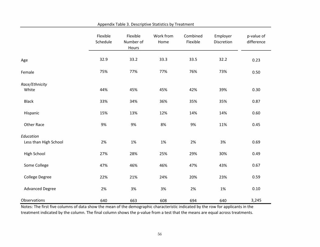
information is related to the wage gap. Appendix Table 3 shows that, consistent with random assignment,

workers in the different treatments have similar demographic characteristics.

4.2 Main Treatments

We begin with visual nonparametric and parametric summaries of the data. We show binned scatterplots

of the inattention-corrected fraction of applicants who chose the arrangement with the amenity, against the

wage gap (4w) between this job and the job without the amenity. We overlay the scatterplot with the ML and

breakpoint model fits, which can be interpreted as cdfs of the WTP distribution since they are monotonic and

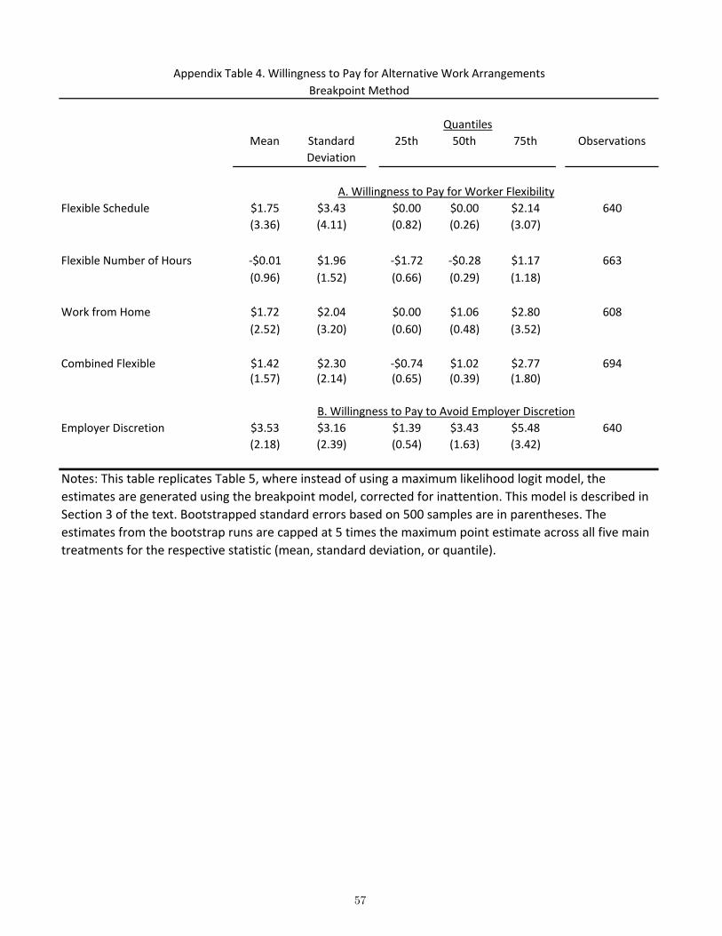
bounded between 0 and 1. We also report statistics from the WTP distribution using the ML model in Table

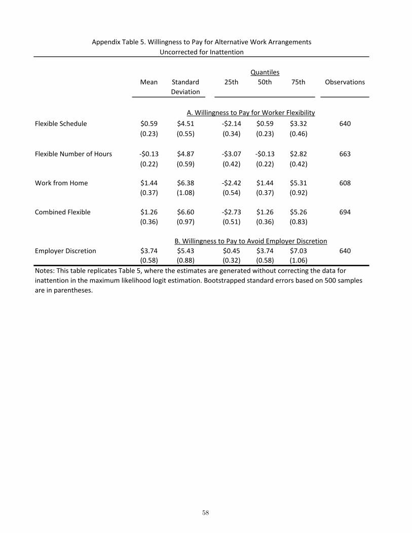
5 and the breakpoint model in Appendix Table 4. Statistics from the ML inattention-uncorrected estimates

are presented in Appendix Table 5 and scatterplots with the uncorrected data are presented primarily in

appendix figures. We discuss the estimates for each of the main alternatives sequentially below.

Flexible Scheduling

The open circles in Figure 1 plot the raw fraction of workers choosing the flexible-schedule job at each

wage gap, without the inattention correction. There is a strong positive relationship between the premium

for the flexible alternative (4w) and the probability that an applicant chose the flexible job. Reading from

this figure where these points intersect the y-axis at 0.5 and multiplying by−1, the median WTP for flexible

scheduling is positive but less than $1 per hour.25 Only 60% of applicants chose the flexible alternative when

4w = 0, suggesting that a large fraction of applicants place no value on this arrangement. In the figure we

can see that when 4w = $5, that is, when the flexible position pays $5 per hour more than the baseline

position, approximately 20% of applicants still choose the fixed position. This gap is expected if there is

inattention. As we discussed above, we fit a line over the range of points between 4w = 2 and 4w = 5

to estimate the share of applicants who choose the dominated position (the baseline position) when it pays

$5 per hour less than the more-flexible position. We do not interpret the share of applicants choosing the

flexible position when 4w is large and negative (that is, when flexibility is more expensive) as reflecting

inattention because there might be applicants who have a strong preference for flexibility.

After estimating the inattention rate using the procedure described above, we calculate the inattention-

corrected shares Y .26 These shares are plotted in the filled circles in Figure 1 along with the estimated

implied cdfs using the ML and breakpoint models. The inattention correction shifts shares that are greater

25The x-axis of this graph shows the wage premium for the job with the higher amenity. Multiplying this by -1 gives the cost ofthe amenity. The cost that 50% of workers is willing to pay is the median WTP.

26Technically these are not shares because they can be greater than 1 or less than 0, but we use this term for convenience.

14

than 0.5 towards 1 and shares that are less than 0.5 towards 0, making the implied cdfs steeper. This changes

the tails of the WTP distribution (where the y-axis meets the lower and upper quantiles) but not the median.

Inspecting this figure we can see that after correcting for inattention almost everyone prefers the flexible

alternative when it pays more, modulo sampling error. This is effectively mechanical at4w = $5, but not at

other values of4w. There is a “cliff” in the cdf at4w = 0, indicating a mass point in the WTP distribution

at this point; approximately 60% of workers do not value being able to make their own schedule at all. The

ML model cannot capture this extreme nonlinearity while the breakpoint model does. In both models most

individuals do not value the ability to make their own schedule and the median WTP for flexible scheduling

is 0 or close to 0. However, there is a tail of individuals who place a high value on this option: the top 25%

of workers – those workers with a WTP in the top 25% of the WTP distribution – are willing to give up

at least 10% of their wages to be able to make their own schedule (Table 5 and Appendix Table 4).27 This

quantitatively and qualitatively important heterogeneity in valuations is something that we observe across

all arrangements we consider. We see a very similar pattern of estimates in the nationally-representative

UAS discussed below.

One potential concern is that at 40 hours per week there may be limited latitude to adjust schedules. To

investigate this possibility, we conducted a supplementary study where we gave workers a choice between

a baseline job and one of our five alternatives, but all jobs were 20 hours per week rather than 40 hours

per week.28 These estimates are reported in Appendix Table 6. The median WTP remains very low in this

part-time alternative: we estimate it at $0.55 (se = $0.50).

The participants in our experiment are a selected sample of workers who responded to our job adver-

tisement. We can construct WTP estimates that match the demographic and education characteristics of

the hourly workforce by reweighting the sample. We construct WTP estimates that weight our sample to

match a nationally-representative sample of hourly workers (those in the 2016 March CPS) using DiNardo,

Fortin and Lemieux (1996) weights. We create two sets of weights: the first uses only the characteristics

collected before participants saw their job options (age, race, and gender) and the second adds educational

attainment categories.29 Descriptive statistics from the March 2016 CPS, our experimental sample, and

our experimental sample reweighted with both sets of weights are in Appendix Table 7. Appendix Table 8

presents willingness to pay estimates using the reweighting. The results are very similar to the estimates

27In the tables we report WTP in levels, as in the experimental variation. We divide our estimates by $17, the approximateaverage wage presented to workers (and the approximate average wage selected) to convert the levels into percentages.

28The flexible number of hours job allows workers to choose the number of hours they work up to 20 hours per week.29To create the first set of weights, we use race dummies, a female indicator, age, age interacted with race dummies, age interacted

with the female dummy, and the female dummy interacted with race dummies. We add educational attainment indicators to createthe second set of weights.

15

using the unweighted data, suggesting that our estimates appear representative of a wider population. This

similarity between the weighted and unweighted estimates is also observed for the other arrangements we

examine. This is largely because as discussed below, aside from by gender, there are not large differences

in WTP by worker characteristics. We provide additional evidence that the estimates are representative in

Section 5 where we report WTP estimates from a discrete choice experiment embedded into a nationally-

representative survey.

The appendix shows the robustness of these results to several different estimation strategies. Appendix

Tables 9 and 10 show the results using different estimates of inattention and estimates of inattention that are

internally estimated in equation 1, respectively.30 Appendix Table 11 limits the sample to (1) workers who

completed the job application, (2) unemployed workers, and (3) workers who were not employed part-time.

Flexible Number of Hours

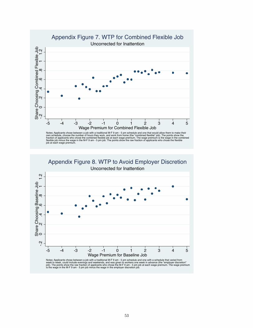
For the remaining treatments, we show the inattention-corrected figures in the text; the uncorrected

versions are in Appendix Figures 5-8. The low valuation for flexibility, on average, is even more striking for

the ability to choose the number of hours worked, as shown in Figure 2. Here the more parsimonious ML

model provides a reasonable fit to the data. The figure shows that the median worker actually slightly prefers

the M-F 9 am - 5 pm job over the ability to choose the number of hours worked. While the median worker

does not value being able to choose the number of hours she works, the top 25% of workers are willing to

give up about 7% of their wages for this flexibility.

We again explore the sensitivity of the estimates to changing the jobs to 20 hour-per-week positions.

This is particularly important for the flexible number of hours comparison because of the possibility that

applicants dislike the flexible option because they believe that the position is less likely to come with benefits.

We eliminate this potential concern by limiting the positions to a maximum of 20 hours. In this 20-hour

version, we see a somewhat higher mean valuation for this alternative (Appendix Table 6), but it remains

small and the median WTP is both insignificantly different from 0 and from the estimate in the 40-hour

version.

Because the negative valuation of the flexible hours arrangement by a subset of applicants is somewhat

puzzling, we created a focus group on Mechanical Turk to help us understand why some people might prefer

less hours flexibility. We gave Mechanical Turk workers the choice between the baseline and flexible hours

position at the same wage and asked them to explain their choice. By virtue of being on Mechanical Turk,

the workers in this survey were much more likely to prefer the flexible number of hours option. However,

30When α is estimated internally, it averages 15.8% across treatments (when allowed to vary only by treatment) and 17.0% (whenallowed to vary by gender and education within treatment), as compared to 14.5% when using the dominated position approach thatwe employ for the main results.

16

the ones who preferred the M-F 9 am - 5 pm job typically mentioned that they liked having someone else

set the schedule and tell them how many hours they should work. They expressed concern that if they could

choose it would be difficult to force themselves to work their desired number of hours.31 This qualitative

evidence suggests that, as previously suggested in Kaur et al. (2015), there may be psychological, not just

economic, factors that enter into the decision over work arrangements.32

The flexible number of hours arrangement offers jobseekers two benefits. It allows workers to make

adjustments if they need to work more or fewer hours in a given week and it allows them to optimize

the number of hours worked if they typically prefer to work fewer than 40 hours. To disentangle these two

possible benefits, and to better understand jobseekers’ labor supply behavior, we designed an auxiliary study

that elicited workers’ preferences over the number of hours of work. We gave applicants choices between

jobs with different wage and hour combinations. We elicited preferences over a 20 versus 40 hour-per-week

position, as before, randomly varying the wage gap between the two jobs such that either wage could be up

to +/− $5 per hour from the other. The higher-paying job paid $16 per hour. Using the above framework,

we can estimate WTP for the 40 hour-per-week job relative to the 20 hour-per-week job. For this exercise,

we specify an inattention rate of α = 0.145 (the mean in our data) rather than estimating it from the share

choosing a dominated position since there is no obvious dominated position for these comparisons.

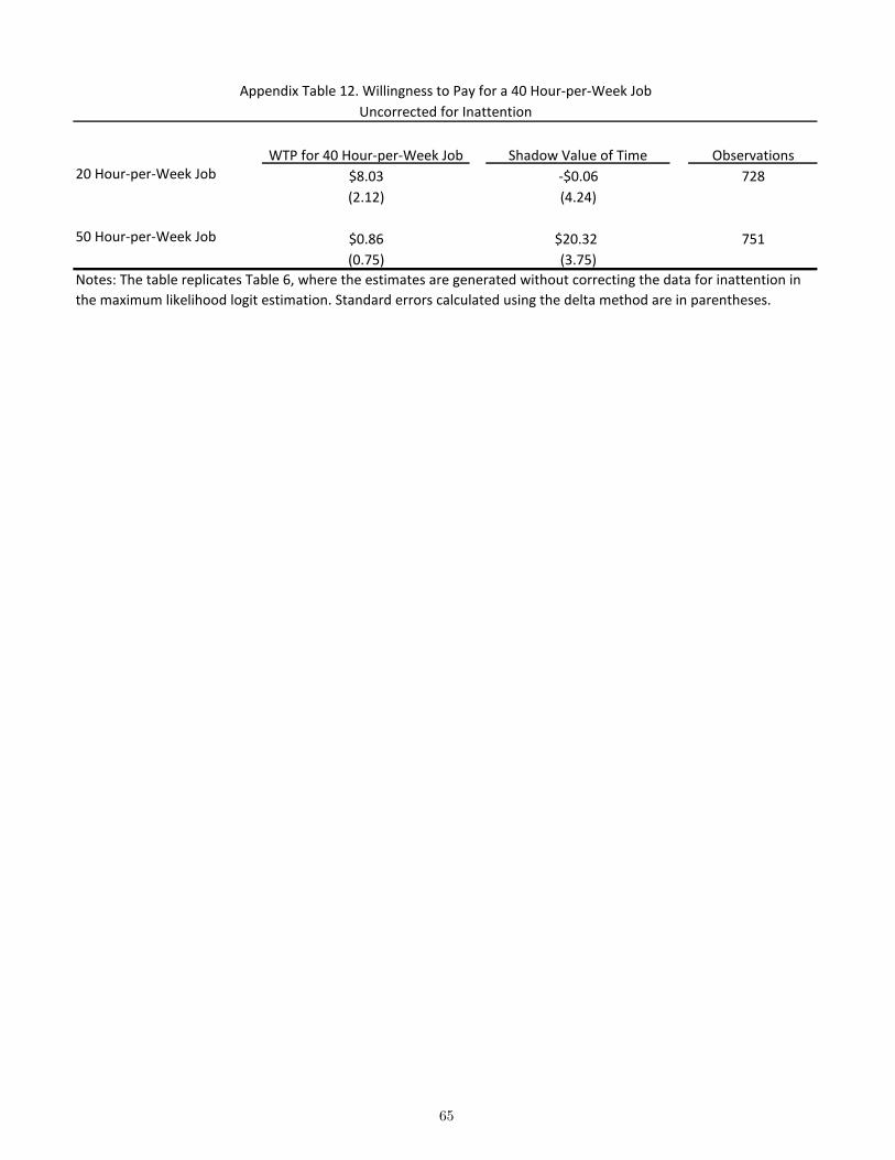
Inattention-corrected WTP estimates are shown in Table 6 and uncorrected estimates are in Appendix

Table 12. At the wages we offer, most workers prefer the 40-hour job: the median worker is willing to take a

$6 per hour pay cut for a 40-hour job relative to a 20-hour job. This implies a median value of time of $4 per

hour between 20 and 40 hours of work.33 Even at the top of the distribution, workers’ value of time is fairly

low. The 75th percentile value of time is approximately $11, well below the predicted market hourly wage

of $16 for the applicant pool.34 In the standard labor supply model, the decision to work part-time when a

worker is unconstrained is due to a high shadow value of time and/or a low wage. Our estimates suggest that

31These are a sample of the responses conditional on choosing the baseline job: “Although being able to choose my hours wouldbe nice, I would kind of have to force myself to work the 40 hours a week;” “I like that the hours and pay are fixed... [with theflexible hours job] I might be tempted to work less hours at the start of [the week] then work longer hours later to compensate ormake enough for that week which would be tiring and stressful;” “I would prefer to have a set schedule every week. A routineis better for me personally;” “[the fixed schedule] suits me better. I like it when someone tells me how long I should work. Thatway there’s an expectation that I can live up to. If I were to choose the hours that I would like to work, it would make me feeluncomfortable and I wouldn’t be sure how the employer would feel about that;” “I prefer to have set hours so I will know for surewhat my schedule will be. This makes it much easier for me to plan other activities and know the expectations.”

32While not mentioned in our focus group, another potential explanation for some workers actually disliking this type of flex-ibility is that it could lead to more work-family conflict or higher expectations from family members for home production (e.g.,Schieman and Young, 2010).

33This value of time is calculated as the amount the worker has to earn per hour in hours 20 through 40 to be indifferent between

the 20 and 40 hour-per-week jobs: 40×(16−WT P)−20×1620 .

34The 75th percentile value of time is calculated using the 25th percentile of the WTP distribution ($2.54 per hour). To calculateapplicants’ predicted market wage, we estimate the average hourly wage in 2016 for hourly workers with the education, race, andgender composition of workers in our sample using CPS data.

17

jobseekers by and large prefer working 40 hours, even at wages substantially lower than the one we offered.

This may explain the very low valuation for hours flexibility since one of its primary benefits (lower regular

hours) appears to be of low value to most jobseekers.

This finding is also relevant for understanding the prevalence of part-time work. In 2016, 23% of workers

worked less than 35 hours per week, and 19% of workers reported working fewer than 35 hours per week

by choice (Flood et al., 2015). With the usual caveats about generalizing, our estimates suggest that most

workers would prefer full-time jobs, with a relatively small fraction preferring part-time work at the same

hourly wage. While this may seem obvious given the distribution of hours, one might have hypothesized

that 40 hour-per-week work hour blocks exceed the preferred hours of many workers due to technological

or organizational constraints. Our experimental evidence suggests this is not the case.

We also investigated preferences for working overtime. Estimating how workers value overtime is par-

ticularly important in the context of the Fair Labor Standards Act (FLSA), which requires employers to pay

most hourly workers time-and-a-half for work over 40 hours per week. To our knowledge, it is not known

how this legislated wage premium compares to workers’ WTP to avoid working these additional hours.

Overtime pay complicates estimating WTP for positions over 40 hours per week. If we presented a 40

versus 50 hours choice without mentioning overtime pay it would be unclear what applicants assume about

overtime pay. To circumvent this problem, we gave some applicants a choice between a 40 hour-per-week

job and a 50 hour-per-week job which both paid the same base wage ($16 per hour). We randomly varied the

overtime premium so that workers would either earn 1.5 × or 2 × wages for hours over 40 hours per week.

Using the fraction of applicants who chose the 50-hour position at the two overtime premia and assuming a

logistic distribution for WTP, we can recover estimates of the WTP distribution.

We have to pay most workers a premium to work over 40 hours: 40 hours appears close to the bliss point

at workers’ predicted market wage. Fifty-five percent of jobseekers accept overtime at 1.5×wages and 66%

accept overtime at 2× wages: the FLSA overtime requirements make the median jobseeker in our applicant

group close to indifferent towards working overtime.35 When assuming a logistic distribution, these rates

imply a WTP to work 40 hours per week of $0.88 in terms of the overall wage (not just for hours over 40).

Workers’ average value of time between 40 and 50 hours of work is over $20 per hour, substantially higher

than their predicted market wage and their value of time before 40 hours of work.

Working from Home

While we see that workers largely do not value choosing the number of hours they work or choosing

which hours these are, applicants do value working from home. The cdf of WTP for this alternative relative

35Both of these rates are inattention-corrected using the average inattention rate in the experiment.

18

to the baseline job is shown in Figure 3. The average worker is willing to give up about 8% of wages for

this option.36 Twenty-five percent of applicants are willing to pay at least $2.45 per hour, or about 14% of

wages, to work from home. Yet, approximately 20% of applicants choose to work exclusively on-site even

when there is no wage penalty for doing so (4w = 0). Bloom et al. (2015) also find that many workers

(50% in the company they study) prefer working on-site, all else equal.37 However, the estimates suggest

that almost no workers are willing to accept a lower wage for the on-site option.

Combined Flexible Option

The distribution of WTP for the option that combines flexible scheduling, flexible number of hours, and

working from home is shown in Figure 4. If these types of flexibility are complements, workers could value

the sum of the components more than the parts. We don’t see evidence supporting this: the mean valuation

of this combined option ($1.17) is close to the sum of its components ($1.59). This approximate equivalence

does, however, provide some reassurance that we are not subjected to the embedding bias of Kahneman and

Knetsch (1992).38 Overall, the combined flexible option looks very similar to the work from home option,

the only worker-friendly alternative that workers seem to value.

Employer Discretion

While most workers seem content to work a regular M-F 9 am - 5 pm job with a fixed schedule and a

set number of hours, they are quite averse to arrangements where the employer has discretion over the work

schedule. As a reminder, we gave workers a choice of a 40 hour-per-week, M-F 9 am - 5 pm job and a 40

hour-per-week job where the employer sets the schedule – which can include evenings and weekends, but

not nights – one week in advance.39 Figure 5 shows the cdfs for the WTP distribution to avoid this option.

Note here that the baseline M-F 9 am - 5 pm job is now the higher amenity position and the y-axis is the

fraction of people who choose the baseline job. The x-axis is the wage difference between the baseline

position and the employer discretion position. For this alternative, the ML and breakpoint models yield an

almost identical fit, suggesting no mass point in the WTP distribution. The average worker is willing to

give up 20% of wages to avoid this employer discretion (Table 5 and Appendix Table 4). And while there

is variation in workers’ aversion to this work arrangement, even the bottom 25% of workers are willing to

give up 10% of earnings to avoid this option. Here we see a similar pattern of estimates in the nationally-

representative UAS study discussed below as well as in the 20 hour-per-week comparisons (Appendix Table

36Estimated mean WTP is about 5% for the 20 hour-per-week version (Appendix Table 6).37The choice we study is slightly different from the one in Bloom et al. (2015) in that our choice provided workers the option of

working from home, not a potential requirement to do so.38The embedding bias occurs when individuals are estimated to have a higher WTP for a good when the good is evaluated on its

own rather than when it is presented as part of a larger, composite good.39In a pilot, we told workers we would give them this schedule two weeks in advance and the results were similar.

19

6).

Workers may dislike employer discretion either because it entails working non-standard hours or because

it requires workers to adjust their schedules on short notice. We use two sets of supplemental treatments

to distinguish between these possibilities. We find that workers have a strong aversion for working non-

standard times, in particular evenings and weekends. However, conditional on working non-standard hours,

they do not appear to dislike having their hours change from week to week or learning their schedules only

a week in advance.

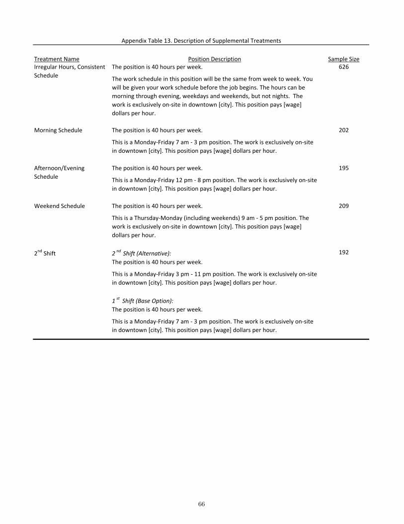
In the first supplementary treatment we gave some workers a choice between a standard M-F 9 am - 5 pm

job and a job with a potentially non-standard schedule that was consistent from week to week. (The exact

wording of this treatment and the others in this section are presented in Appendix Table 13.) The position

description stated that the work schedule would be the same from week to week, but would be determined

at a future time, before the job begins.40 This job differs from the employer discretion job only in that in

this job the hours are the same from week to week, while in the employer discretion job, the schedule can

change from week to week and workers are only guaranteed a week’s notice of their schedule. Despite the

fact that this job came with consistency and ability for more advanced planning, the average worker required

the same amount to take this job (20%) as they did for the employer discretion job (Table 7). This points to

the non-standard work schedule as the more likely reason for the strong distaste for irregular jobs.

We test workers’ aversion to non-standard schedules directly in the second set of supplementary treat-

ments. Here we elicit preferences for schedules that involve working alternative times and days. We gave

workers a choice between our baseline M-F 9 am - 5 pm job and jobs with consistent alternative schedules:

(1) Monday - Friday 7 am - 3 pm, (2) Monday - Friday 12 pm - 8 pm, and (3) Thursday - Monday (including

weekends) 9 am - 5 pm. On average, workers like the 7 am - 3 pm schedule. However, they dislike working

evenings and weekends. The average worker requires 14% more to work evenings and 19% more to work

weekends. It is interesting that the point estimate for the mean WTP to avoid weekend work ($3.27) is

very close to the corresponding point estimate to avoid employer discretion ($3.41). This pattern further

reinforces the conclusion that the aversion to employer discretion is rooted in a distaste for non-standard

work schedules. These findings are also helpful in that these very differently-worded comparisons lead us to

the same conclusions, quantitatively and qualitatively, suggesting internal consistency in the experimental

approach.41

40The schedule in this job was described as follows: “The work schedule in this position will be the same from week to week.You will be given your work schedule before the job begins. The hours can be morning through evening, weekdays and weekends,but not nights.”

41Diamond (1996) recommends testing for internal consistency in contingent valuation surveys. We go further in Section 5 bycomparing WTP estimates in the market setting to estimates from a nationally-representative survey.

20

We also estimate workers’ willingness to pay to work the “1st shift” (M-F 7 am - 3 pm) relative to the

“2nd shift” (M - F 3 pm - 11 pm), by having workers choose between these two options. We find that

workers strongly prefer the first to the second shift. Even the 25% of workers who least dislike the later

shift require approximately 8% more to work the 2nd shift. This is larger than the 2nd shift wage premium

reported in employer surveys. These surveys tend to find that only a relatively small share of employers has

a 2nd shift premium, and when they do it is in the 5%−10% range (Aguirre and Moore-Ede, 2014).

5 Understanding America Study

To further probe the external validity of our experimental results, we designed a survey to elicit valuations of

work arrangements from participants in the nationally-representative Understanding America Study.42 We

focus on three work arrangements: flexible scheduling, working from home, and employer discretion.

All employed and unemployed respondents were asked to consider the following scenario about an

employer discretion job:

Imagine that you are applying for a new job in your [current line of work, same line of work as your last

job], and you have been offered two positions. Both positions are the same as your [current/last] job in all

ways, and to each other, other than the work schedule and how much they pay. ¶ Please read the

descriptions of the positions below. ¶ Position 1) This position is 40 hours per week. The work schedule is

Monday - Friday 9am - 5pm. This position pays the same as your [current/last] job. ¶ Position 2) This

position is 40 hours per week. The work schedule in this position varies from week to week. You will be

given your work schedule one week in advance by your employer. The hours can be morning through

evening, weekdays and weekends, but not nights. ¶ This position pays “X” your current job. ¶ Which

position would you choose?

Here, [current/last] is “current” for employed workers and “last” for unemployed workers. Employed

workers were instructed that these positions were in their current line of work, while unemployed

respondents were told the positions were in the same line of work as their last job. For employed workers

“X” randomly varies between “30% less than,” “the same as,” “2% more than,” “5% more than,” “10%

42The UAS is an internet survey run out of the University of Southern California and established and directed by Arie Kapteyn.It consists of a panel of respondents who were randomly selected to participate in an ongoing web-based survey. Because it wasestablished in 2013, there are only a small number of papers that have utilized the survey, but it is closely related in design to theRand American Life Panel which has a long track record. See here for further details: https://uasdata.usc.edu/.

21

more than,” “15% more than,” “25% more than,” and “35% more than.”43 These values were chosen to

match the values used in our experiment, where the largest wage gap offered was 31%. We used fewer

values of X – “5% more than,” “15% more than”, and “35% more than,” – for the unemployed group since

it is a much smaller sample. We use workers’ choices when the employer discretion job pays 30% less than

the Monday - Friday 9 am - 5 pm job to measure inattention. As in our experiment, we assume that workers

choosing the employer discretion job when it pays 30% less are inattentive. We randomized whether the

employer discretion position was Position 1 or Position 2.

We ask workers a similar question to elicit their WTP to work from home, with two adjustments. First,

we allow for the possibility that some workers cannot do their jobs from home. We first ask workers,

regardless of where they actually work, what fraction of their work could feasibly be completed from home.

If they answered at least 10%, our hypothetical positions are described as being in the workers’ current line

of work and the same as their current job in all ways other than the work location and pay. If less than 10%

of their work could be completed from home, we describe the jobs as being a new line of work.44 Second,

to determine the effect of travel time on WTP for working from home, we randomize the one-way commute

time “Y”. We chose the commute times, 10, 20, 30, and 40 minutes, to match the mean commute time in the

experimental sample and use the same values of “X” as in the employer discretion question.

Imagine that you are applying for a new job in [your current line of work, the same line of work as your

last job, a different line of work] and you have been offered two positions. Both positions are the same [as

your current main job, as your last job] in all ways and to each other, other than the work location and how

much they pay. Please read the descriptions of the positions below. ¶ Position 1) This position has the same

schedule as your [current, last] job. In this job, you have the option of working from home as well as on-site

“Y” minutes from your home. This position pays the same as your [current, last] job. ¶ Position 2) This

position has the same schedule as your [current, last] job. This job requires you to work exclusively on-site

“Y” minutes from your home. ¶ This position pays “X” your [current, last] job. ¶ Which position would

you choose?

To elicit WTP for flexible scheduling, we first ask respondents whether they can choose the days and

times that they work. Unemployed and self-employed respondents are not included. If the respondent

reports having a flexible job, we ask:

Suppose your primary employer gives you the option of working a fixed work schedule, Monday-Friday43We also clarify that “By pay we mean your salary if you [are,were] a salaried employee or your hourly pay if you [are,were]

an hourly employee. If you [are,were] a part-time salaried employee we mean the salary you would have received if working on afull-time basis.”

44Unemployed workers are asked this question about their previous job and treated accordingly.

22

during the daytime. Under this arrangement you would continue to work your usual number of hours but

once your schedule is set you may not change the times and days of work. In exchange for having this fixed

rather than flexible schedule you would get [2/5/10/20/35]% higher pay. Would you agree to this

arrangement if given the choice?

If the respondent does not report having a flexible job we ask:

Suppose your primary employer gives you the option of being able to make your own work schedule.

Under this arrangement, you would continue to work your usual number of hours but you may freely

choose the times and days you work. In exchange for having this flexible rather than fixed schedule you

would get [2/5/10/20/35]% lower pay. Would you agree to this arrangement if given the choice?

The UAS allows us to ask about the presence of children in the home, which seemed inappropriate on a

job application. The survey targeted 2,318 respondents and the response rate was 84%.45

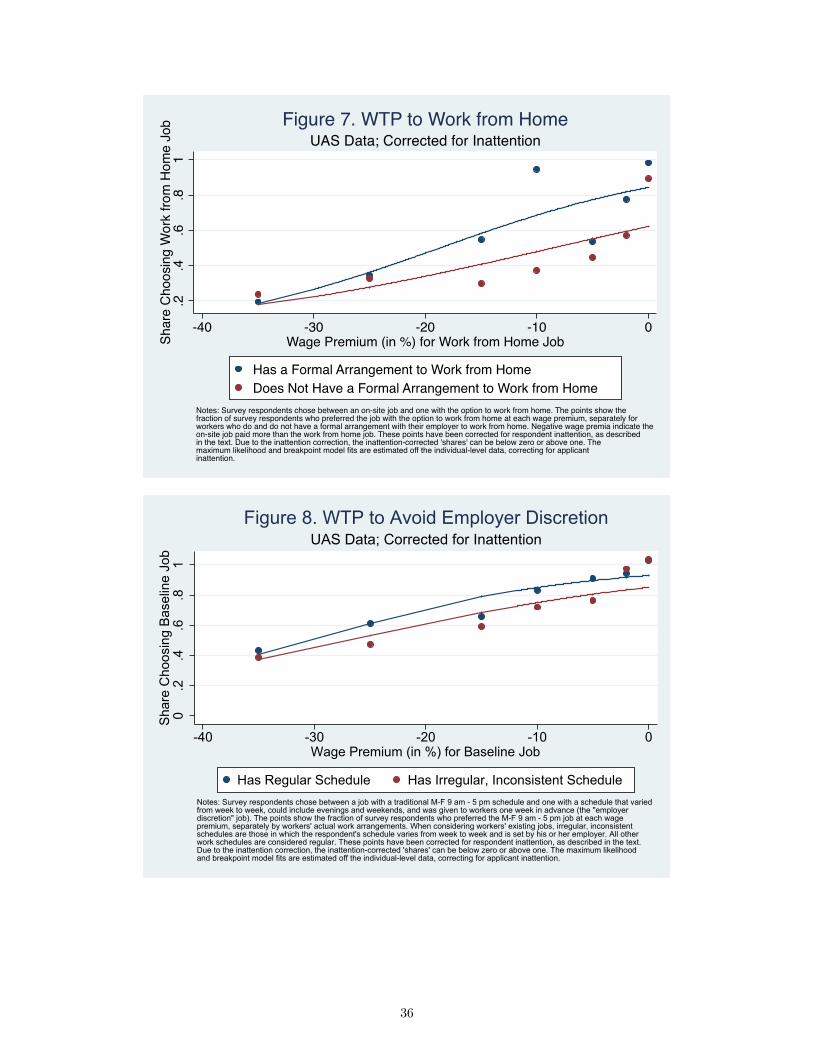
We present the findings in two ways. We show figures like the ones for job applicants, plotting the share

of respondents who selected either the baseline position (in the baseline vs. employer discretion comparison)

or the work-from-home or flexible-schedule position. We also estimate inattention-corrected ML models,

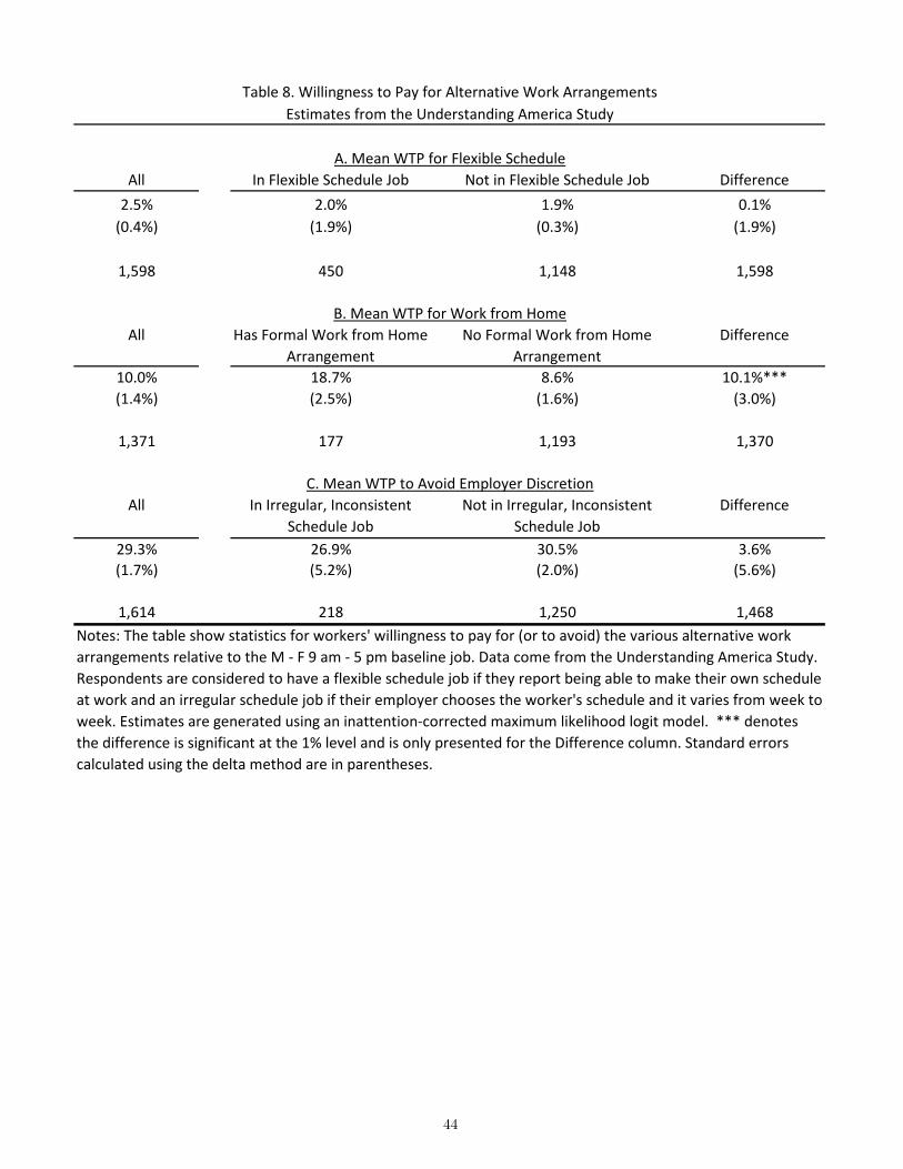
as above, to quantify valuations over these alternatives (Table 8). In the UAS, workers’ average willingness

to pay for flexible scheduling was 2.5% of wages, relative to 2.8% in our experimental data. This argues

against the concern that experimental participants disguised their desire for flexibility to be more appealing

applicants. We designed our choice page to explicitly eliminate this concern – assuring applicants that (1)

their choice would not affect whether they were hired, but only what job they were matched to and (2)

their choice would be reviewed only after hiring decisions were made. Applicants’ willingness to avoid

the employer discretion job also suggests that they were not simply choosing the most-palatable job to

employers.

Figure 6 plots the choices for the flexible-schedule job for survey respondents not in flexible-schedule

jobs. There is very little demand in this group for flexible positions; only half of respondents are willing to

take even a 2% pay cut for flexibility. Among individuals currently in positions with flexible scheduling, it is

more nuanced. While the mean WTP is still quite low among this group (2.0%), there is a subset of workers

that really values flexibility. The top 25% of workers in flexible jobs is willing to give up 16% of their pay

for the option to make their own schedule. This is consistent with sorting in the labor market, where workers

with the highest WTP for flexible scheduling are in flexible-schedule jobs.46 This may also be driven by the45We added the work from home questions in a later module. We targeted the same individuals, but the response rate was 74%.46Past evidence on sorting into job attributes based on preferences includes Viscusi and Hersch (2001), Borghans et al. (2006),

and Krueger and Schkade (2008).

23

endowment effect, with workers valuing the ability to make their own schedules because they have it.

Figure 7 plots the WTP to work from home separately for workers with and without formal work from

home arrangements. Overall, mean WTP for this type of flexibility (10.0%) is similar to the WTP we

estimate in the experiment. When we re-weight WTP in the UAS by the distribution of workers’ actual

commute times in the experiment, we get an average WTP for working at home of 8.4%, very similar to the

7.8% we obtain in the experiment. Consistent with labor market sorting, workers with formal work-from-

home arrangements are willing to pay significantly more (18.7% of wages vs. 8.6%) for this option. We

also estimate the impact of randomly-assigned travel time on the WTP for home work in the UAS (Table 9).

WTP for working from home is relatively similar when workers have 10- and 20-minute one-way commutes

(6.9% and 7.4%, respectively). It starts increasing when workers have to travel at least an hour round-trip.

We also estimated WTP in the field study by workers’ estimated actual commute time to the job. For this

exercise we used workers’ zip codes and the Google Maps API to calculate the typical driving time to the

downtown area of each worker’s metro area (where the job was said to be located) on a Monday at 8 am.

Most workers who applied to the position were relatively close to the stated work location; 75% had less

than a 25 minute one-way commute and only 12% live more than 35 minutes away. Due to the low number

of longer distance commuters, we cannot obtain precise estimates on how WTP varies by commute time in

the field.

Table 8 shows the additional wages workers need to accept a job with employer discretion. The estimated

mean WTP to avoid employer discretion in the survey is 29.3% as compared to 23.1% in the field study.

Amongst unemployed workers in the UAS, WTP to avoid employer discretion is almost identical to the field

study (22.7%).47 Consistent with labor market sorting, the average worker in an employer discretion job is

less averse to this job than is the average worker in a job without employer discretion, though this difference

is not significant (Table 8). Nevertheless, workers in jobs with employer discretion would be willing to give

up a significant fraction of their wages for M-F 9 am - 5 pm jobs: the top 25% of workers would give up

at least 43% of their earnings (Figure 8). This suggests the presence of frictions or other job characteristics

that prevent perfect sorting.

6 Heterogeneity in Valuations

A number of papers suggest that women value flexibility and standard work schedules more than do men

(e.g., Wiswall and Zafar, 2016) and that this may explain gender wage gaps (e.g., Goldin and Katz, 2011

47While one might have worried that many experimental participants were unemployed because they dislike employer discretion,unemployed workers do not dislike employer discretion more than do employed workers.

24

and Cortes and Pan, 2016). We find that women do have a higher valuation for worker-friendly work

arrangements and a stronger distaste for employer discretion than do men. However, the differences in work

schedules by gender along these margins are not large enough to explain a substantial part of gender wage

gaps.

Table 10 shows mean willingness to pay by gender for the five main alternative work arrangements in

our field experiment and Appendix Table 14 shows the quantiles of the WTP distributions. On average,

neither men nor women are willing to pay much for flexibility in their schedules or in the number of hours

they work. While we do not have information on whether the workers in our experiment have children, we

do have this information for workers in the UAS. Table 11 shows that, on average, even women with young

children (under four years of age), are not willing to take a pay cut for flexible scheduling. Even at the upper

quantiles of the distribution, women with young children do not have higher WTP for flexible scheduling

than do men. This is consistent with the fact that women with young children are not more likely to be in

jobs with flexible schedules (Table 11).

While women do not seem to value the flexibility to adjust their schedule from the traditional M-F 9 am

- 5 pm schedule, they do seem to be willing to pay substantially more than are men for the ability to work

from home (more than twice as much, though this difference is not statistically significant). They are also

willing to pay more for the combined flexible job. And women are willing to pay twice as much as are men

to avoid employer discretion (Table 10). In particular, in the UAS, we find that women with young kids are

willing to give up almost 40% of their wages to avoid a job with an irregular schedule. Unlike women, men

with young children are not willing to pay more than other men to avoid a non-standard schedule (Table 11).

Women with young children also appear to have a higher WTP to work from home than do other women.48

As we would expect based on their preferences, women are more likely to work from home (12.9% of

female and 7.3% of male hourly workers have a formal work-from-home arrangement). Women are also

less likely to be in jobs with inconsistent, irregular schedules (16.6% of women vs. 19.3% of men). These

gaps change to 4.4% and 5.7%, respectively when controlling for education, race and ethnicity, age, marital

status, self-employment, and part-time work.49 However, because the difference in the prevalence of these

arrangements by gender is so small, even with sizable compensating differentials, these differences cannot

48Our results are similar when we consider children of different ages. For all ages up to 18, we find women with children thatage or younger have a higher WTP to avoid employer discretion than do other women. The difference is significant at the 5% levelonly for children under three years old. Women with young children are never willing to pay more for flexible scheduling than areother women, regardless of the age cutoff we use. And women with young children always have a higher WTP to work at homethan do other women, but this difference is only ever significant at the 10% level.

49These statistics come from the UAS. They differ from the prevalence numbers in Table 11 since here we consider only hourlyworkers, for whom we think our experiment is most representative. Using all workers in the UAS, women are 2.6 percentage pointsmore likely to have a work-from-home arrangement (1.3 percentage points with controls) and 5.2 percentage points less likely tohave an inconsistent, irregular schedule (7.6 percentage points with controls).

25

explain large gender wage gaps. For example, with a 20% compensating differential for both work at home

and working a fixed schedule instead of an irregular one, the differences by gender in the prevalence of these

arrangements would only lead to a 1.7% raw gender wage gap or a 2.0% gap with controls.

While we do find large differences by gender in WTP for alternative work arrangements, we do not find

significant or consistently-signed differences by the other characteristics we have: ethnicity, age, education,

number of ACT WorkKeys questions answered correctly (experimental data only), or family income (UAS

data only). Appendix Table 15 shows the differences in WTP for alternative work arrangements for these

subgroups.

Table 12 presents results from regressions of whether the applicant chose the more-flexible job on worker

characteristics. We limit the regression to choices in our main treatments where the more-flexible job had a

lower wage. (In the employer discretion treatment, the more-flexible job is the baseline job.) We control for

the wage gap 4w. Consistent with our other results, workers choosing worker-friendly arrangements are

more likely to be female, but they look similar on other characteristics.

7 Discussion and Conclusion

We implement a discrete choice experiment in the job application process for a national call center to es-

timate workers’ willingness to pay for alternative work arrangements. Despite widely held views on the

importance of workplace flexibility (see e.g., Dominus, 2016), the majority of workers do not value flexible

scheduling or the ability to choose the number of hours they work. Workers do value the option to work from

home and strongly dislike employers setting their schedules on short notice, mainly because they don’t want

to work evenings and weekends. Overall, the traditional M-F 9 am – 5 pm schedule works well for most

people, perhaps because this schedule allows them to coordinate their leisure time. Despite these strong

preferences for traditional hours, the incidence of odd hour work is high in the United States. Hamermesh

and Stancanelli (2015) find that adjusting for demographics and number of hours worked, workers in the

United States are far more likely to work unusual hours than workers in continental Europe.

We find that jobseeker aversion to irregular schedules appears to be rooted more in their distaste for

evening and weekend work than inconsistency of schedules. This may be surprising given the amount of

recent policy attention to providing workers with predictability and stability in scheduling. For example, San

Francisco and Seattle have recently passed laws that require some employers to give workers their schedules

with two weeks notice and pay workers additional “predictability pay” if they change schedules within this

window (Tu, 2016 and Sahadi, 2014). In 2015, the New York attorney general investigated 13 large firms

26

for giving workers their schedules on too-short notice (Tabuchi, 2015). Meanwhile, Starbucks changed its

policies to provide baristas with at least one week of advanced scheduling (Kantor, 2014), while Walmart

provided some workers with fixed shifts with the same hours each week (DePillis, 2016). We note, however,

that our experiment does not include any jobs with on-call scheduling or in which workers learn their shifts

less than a week in advance. Workers may still have a strong aversion to these scheduling practices.

Our estimates of the WTP distribution for workplace amenities allow us to shed light on market compen-

sating differentials. For all of the job attributes we consider, there is considerable evidence of heterogeneity

in valuations, suggesting that any analysis based on mean WTP alone will lead to possibly misleading con-

clusions. While scheduling flexibility is not valued by most workers, the right tail in the WTP distribution

still allows for potentially large market compensating wage differentials. The estimates imply that an em-

ployer could set the wage of a flexible-schedule job or a work-from-home job at 11% or 14% below the

market wage of a fixed-schedule job, respectively, and still attract at least 25% of the applicants who would

have applied to the fixed-schedule job at the higher wage.

Whether there is a business case for setting lower wages and providing this flexibility depends on a

number of things, including the relative productivity of workers with high WTP. In the Chinese firm studied

by Bloom et al. (2015), workers who chose to work from home appear at least as productive ex ante as

workers who did not. In our experiment, workers who select into flexible positions differ significantly

only in their gender; they have similar educational characteristics and scores on the cognitive application

questions as workers choosing less-flexible positions (Table 12). Another important factor is the extent to

which a firm can distinguish higher-ability applicants with a high WTP for these arrangements from lower-

ability workers since setting a lower wage would mean attracting more lower-ability applicants. A firm

would also need to consider the impact of these arrangements on worker productivity, turnover, and capital

costs.50

Alternatively, we can interpret our estimates as providing the WTP distribution for the overall workforce

(or the population of hourly workers). There is evidence that this is a reasonable approximation given the

close correspondence between the weighted and unweighted estimates, and the experimental and nationally-

representative survey estimates. Viewed this way, the WTP distributions shed light on the cost to firms

of alternative work arrangements. In the frictionless Rosen (1986) framework, workers with the highest

valuations for an amenity work at firms with the lowest cost of providing it. These firms provide the amenity,

while higher-cost firms employing lower-valuation workers do not. The market compensating differential is

50In a randomized experiment, Bloom et al. (2015) find that working from home increased the productivity of call center workersin a Chinese company. Moen et al. (2016) experimentally evaluate the effects of greater employee control over work time in a U.S.company and find evidence of higher job satisfaction and lower stress among employees.

27

the marginal worker’s valuation of the amenity, or equivalently, the marginal firm’s cost of providing it.

Taking our estimated distribution of WTP as the market distribution, we can calculate the implied market

compensating differential for an attribute by inverting E[Y | 4w

]. Under perfect sorting, if p is the share of

workers in the alternative arrangement, the marginal worker’s valuation is the 1− p percentile of the WTP

distribution. This is of course not meant to be taken literally as the actual market compensating differential –

there are many reasons why such differentials may not appear – but it is a useful way to assess magnitudes.51

In the UAS survey, 20% of hourly workers report being able to make their own schedules. Based on

our estimates, there are still workers on the margin who would choose flexible scheduling at a 12% wage

discount. The fact that employers are not offering these marginal workers flexible scheduling suggests that

flexible scheduling is quite costly for the marginal employer to implement. To the extent that there is not

perfect sorting of workers to firms based on the value of the amenity, this conclusion is amplified: there are

workers in inflexible jobs willing to take even larger pay cuts for flexible scheduling.52 Offering flexible

scheduling could be costly to firms because it leads to difficulties in worker coordination or in the ability to

monitor workers.

We can do a similar calculation for the ability to choose the number of hours worked. Given that 18%

of hourly workers in the UAS report being able to choose the number of hours they work, this suggests a

market compensating differential of 10% – a sizable compensating differential even given that the average

worker does not value this type of flexibility.

Despite the fact that the average worker places a relatively high valuation on working from home, only a

relatively small share of hourly workers (10% in the UAS) has a formal work-from-home arrangement. This

suggests that there are workers who don’t have this option who would be willing to take 21% lower wages

for the ability to work from home. The fact that they are not working from home suggests that it is likely

quite costly for employers to implement this type of flexibility.53

Women value working from home and dislike employer discretion more than men do. However, because

men are only slightly less likely to work from home and slightly more likely to work irregular schedules,

51In the presence of frictions, there may be no market compensating differential, even if workers have an aversion to a jobattribute. Our finding of heterogenous valuations provides support for the general case of the Lang and Majumdar (2004) matchingmodel which can explain the absense of compensating differentials, the low incidence of job amentities, and the potential forpareto-improving regulations on workplace conditions.

52One caveat is that firms may be prevented from lowering wages by the minimum wage. However, in the UAS we find that theprevalence of and WTP for flexible scheduling are similar when we restrict attention to workers earning above-minimum wages.

53This may be surprising given the positive benefits of work from home found in Bloom et al. (2015). Some jobs (e.g., operatinga cash register) cannot be conducted from home and many others may require more cooperation and teamwork, potentially reducingthe benefits of home work. Alternatively, many employers may overestimate the costs of providing worker flexibility. Altman andGolden (2007) and Hohl (2015) also suggest that flexible scheduling may reduce firms’ costs (e.g., by reducing turnover) or have anegligible effect on costs.

28

even with large compensating differentials, these differences in preferences cannot explain a large part of

gender wage gaps.

References

Abaluck, Jason and Jonathan Gruber, “Choice inconsistencies among the elderly: evidence from planchoice in the Medicare Part D program,” The American Economic Review, 2011, 101 (4), 1180–1210.

Aguirre, Acacia and Andrew Moore-Ede, “Shiftwork Practices 2014 Manufacturing,” Circadian Infor-mation, 2014.

Bloom, Nicholas, James Liang, John Roberts, and Zhichun Jenny Ying, “Does Working from HomeWork? Evidence from a Chinese Experiment,” The Quarterly Journal of Economics, 2015, 165, 218.

Bonhomme, Stèphane and Grègory Jolivet, “The Pervasive Absence of Compensating Differentials,”Journal of Applied Econometrics, 2009, 24 (5), 763–795.

Borghans, Lex, Bas Ter Weel, and Bruce A Weinberg, “People people: Social capital and the labor-market outcomes of underrepresented groups,” Technical Report, National Bureau of Economic Research2006.

Brown, Charles, “Equalizing Differences in the Labor Market,” The Quarterly Journal of Economics, 1980,pp. 113–134.

Card, David, “The effect of unions on the structure of wages: A longitudinal analysis,” Econometrica:Journal of the Econometric Society, 1996, pp. 957–979.

Chetty, Raj, Adam Looney, and Kory Kroft, “Salience and taxation: Theory and evidence,” The Americaneconomic review, 2009, 99 (4), 1145–1177.

Cortes, Patricia and Jessica Pan, “When Time Binds: Returns to Working Long Hours and the GenderWage Gap among the Highly Skilled,” 2016.

Council of Economic Advisors, “Work-Life Balance and the Economics of Workplace Flexibility,” March2010. https://www.whitehouse.gov/files/documents/100331-cea-economics-workplace-flexibility.pdf.

DellaVigna, Stefano, “Psychology and economics: Evidence from the field,” Journal of Economic litera-ture, 2009, 47 (2), 315–372.

Deloitte, “Workplace of the Future: Creating an Elastic Workplace,” Human Capital Trends, 2013.https://www2.deloitte.com/content/dam/Deloitte/global/Documents/HumanCapital/dttl-humancapital-trends5-workplaces-no-exp.pdf.

DePillis, Lydia, “Walmart Is Rolling out Big Changes to Worker Schedules This Year,” Washington Post,February 2016.

Diamond, Peter, “Testing the Internal Consistency of Contingent Valuation Surveys,” Journal of Environ-mental Economics and Management, 1996, 30 (3), 337–347.

Diamond, Peter A and Jerry A Hausman, “Contingent Valuation: Is Some Number Better Than NoNumber?,” The Journal of Economic Perspectives, 1994, 8 (4), 45–64.

29

DiNardo, John, Nicole M Fortin, and Thomas Lemieux, “Labor Market Institutions and the Distributionof Wages, 1973-1992: A Semiparametric Approach,” Econometrica, 1996, 64 (5), 1001–1044.

Dominus, Susan, “Rethinking the Work-Life Equation,” New York Times Magazine, February 2016.https://www.nytimes.com/2016/02/28/magazine/rethinking-the-work-life-equation.html.

Eriksson, Tor and Nicolai Kristensen, “Wages or fringes? Some evidence on trade-offs and sorting,”Journal of Labor Economics, 2014, 32 (4), 899–928.

Ferrell, Diana and Fiona Greig, “Paychecks, Paydays and the Online Platform Economy,” JPMorganChase & Co. Institute, February 2016.

Filer, Randall K, “Male-Female Wage Differences: The Importance of Compensating Differentials,” In-dustrial & Labor Relations Review, 1985, 38 (3), 426–437.

Flood, Sarah, Miriam King, Steven Ruggles, and J. Robert Warren, “Integrated Public Use MicrodataSeries, Current Population Survey: Version 4.0,” [Dataset], Minneapolis: University of Minnesota, 2015.http://doi.org/10.18128/D030.V4.0.

Flory, Jeffrey A, Andreas Leibbrandt, and John A List, “Do Competitive Workplaces Deter FemaleWorkers? A Large-Scale Natural Field Experiment on Job-Entry Decisions,” The Review of EconomicStudies, 2015, pp. 122–155.

Gariety, Bonnie Sue and Sherrill Shaffer, “Wage Differentials Associated with Flextime,” Monthly LaborReview, 2001, 124, 68.

and , “Wage Differentials Associated with Working at Home,” Monthly Labor Review, March 2007,pp. 61–67.

Goddeeris, John H, “Compensating Differentials and Self-Selection: An Application to Lawyers,” TheJournal of Political Economy, 1988, pp. 411–428.

Goldin, Claudia, “A Grand Gender Convergence: Its Last Chapter,” The American Economic Review, 2014,104 (4), 1091–1119.

and Lawrence F Katz, “The Cost of Workplace Flexibility for High-Powered Professionals,” The Annalsof the American Academy of Political and Social Science, 2011, 638 (1), 45–67.

and , “A Most Egalitarian Profession: Pharmacy and the Evolution of a Family-Friendly Occupation,”Journal of Labor Economics, 2016, 34 (3), 705–745.

Hall, Robert E and Andreas I Mueller, “Wage Dispersion and Search Behavior,” Technical Report, Na-tional Bureau of Economic Research 2015.

Hamermesh, Daniel S and Elena Stancanelli, “Long Workweeks and Strange Hours,” ILR Review, 2015,68 (5), 1007–1018.

Hanley, Nick, Robert E Wright, and Vic Adamowicz, “Using Choice Experiments to Value the Environ-ment,” Environmental and Resource Economics, 1998, 11 (3-4), 413–428.

Hausman, Jerry A, Jason Abrevaya, and Fiona M Scott-Morton, “Misclassification of the DependentVariable in a Discrete-Response Setting,” Journal of Econometrics, 1998, 87 (2), 239–269.

30

Hedegaard, Morten and Jean-Robert Tyran, “The Price of Prejudice,” Technical Report, University ofCopenhagen Department of Economics 2014.

Hwang, Hae-shin, Dale T Mortensen, and W Robert Reed, “Hedonic Wages and Labor Market Search,”Journal of Labor Economics, 1998, 16 (4), 815–847.

Johnson, F Reed, Emily Lancsar, Deborah Marshall, Vikram Kilambi, Axel Mühlbacher, Dean ARegier, Brian W Bresnahan, Barbara Kanninen, and John FP Bridges, “Constructing experimentaldesigns for discrete-choice experiments: report of the ISPOR conjoint analysis experimental design goodresearch practices task force,” Value in Health, 2013, 16 (1), 3–13.

Kahneman, Daniel and Jack L Knetsch, “Valuing Public Goods: The Purchase of Moral Satisfaction,”Journal of Environmental Economics and Management, 1992, 22 (1), 57–70.

Kantor, Jodi, “Starbucks to Revise Policies to End Irregular Schedules for Its 130,000 Baristas,” NewYork Times, August 2014. https://www.nytimes.com/2014/08/15/us/starbucks-to-revise-work-scheduling-policies.html.

Katz, Lawrence F and Alan B Krueger, “The Rise and Nature of Alternative Work Arrangements in theUnited States, 1995-2015,” 2016.

Kaur, Supreet, Michael Kremer, and Sendhil Mullainathan, “Self-control at work,” Journal of PoliticalEconomy, 2015, 123 (6), 1227–1277.

Kostiuk, Peter F, “Compensating Differentials for Shift Work,” Journal of Political Economy, 1990,pp. 1054–1075.

Krueger, Alan B and David Schkade, “Sorting in the Labor Market Do Gregarious Workers Flock toInteractive Jobs?,” Journal of Human Resources, 2008, 43 (4), 859–883.

Lanfranchi, Joseph, Henry Ohlsson, and Ali Skalli, “Compensating Wage Differentials and Shift WorkPreferences,” Economics Letters, 2002, 74 (3), 393–398.

Lang, Kevin and Sumon Majumdar, “The Pricing of Job Characteristics When Markets Do Not Clear:Theory and Policy Implications,” International Economic Review, 2004, 45 (4), 1111–1128.

List, John A and Jason F Shogren, “Calibration of the difference between actual and hypothetical valua-tions in a field experiment,” Journal of Economic Behavior & Organization, 1998, 37 (2), 193–205.

Manski, Charles F, “The Structure of Random Utility Models,” Theory and Decision, 1977, 8 (3), 229–254.

McFadden, Daniel, “Conditional Logit Analysis of Qualitative Choice Behavior,” in Paul Zarembka, ed.,Frontiers in Econometrics, Academic press, 1973, chapter 4, pp. 105–142.

Moen, Phyllis, Erin L. Kelly, Wen Fan, Shi-Rong Lee, David Almeida, Ellen Kossek, and Orfeu Bux-ton, “Does a Flexibility/Support Organizational Initiative Improve High-Tech Employees’ Well-Being?Evidence from the Work, Family, and Health Network,” American Sociological Review, 2016, 81 (1),134–164.

Oettinger, Gerald S, “The Incidence and Wage Consequences of Home-Based Work in the United States,1980–2000,” Journal of Human Resources, 2011, 46 (2), 237–260.

Rosen, Sherwin, “Hedonic Prices and Implicit Markets: Product Differentiation in Pure Competition,”Journal of Political Economy, 1974, 82 (1), 34–55.

31

, “The Theory of Equalizing Differences,” Handbook of Labor Economics, 1986, 1, 641–692.

Sahadi, Jeanne, “San Francisco Passes Retail Worker ‘Bill of Rights’,” CNN Money, December 2014.http://money.cnn.com/2014/11/26/pf/san-francisco-retail-restaurant-workers/.

Schieman, Scott and Marisa Young, “Is There a Downside to Schedule Control for the Work-FamilyInterface?,” Journal of Family Issues, 2010, 31 (10), 1391–1414.

Smith, Robert S, “Compensating Wage Differentials and Public Policy: A Review,” Industrial and LaborRelations Review, 1979, pp. 339–352.

Sorkin, Isaac, “Ranking Firms Using Revealed Preference,” 2015.

Stern, Scott, “Do Scientists Pay to Be Scientists?,” Management Science, 2004, 50 (6), 835–853.

Taber, Christopher and Rune Vejlin, “Estimation of a Roy/Search/Compensating Differential Model ofthe Labor Market,” Technical Report, National Bureau of Economic Research 2016.

Tabuchi, Hiroko, “Retailers Scrutinized for Schedules And Staffing,” New York Times, April 2015.https://www.nytimes.com/2015/04/13/business/retailers-scrutinized-for-schedules-and-staffing.html.

Tu, Janet I., “Seattle City Council Approves Worker-Scheduling Law,” The Seattle Times, September 2016.http://www.seattletimes.com/business/retail/seattle-council-approves-worker-scheduling-law/.

Viscusi, W Kip and Joni Hersch, “Cigarette smokers as job risk takers,” Review of Economics and Statis-tics, 2001, 83 (2), 269–280.

and Joseph E Aldy, “The Value of a Statistical Life: A Critical Review of Market Estimates Throughoutthe World,” Journal of Risk and Uncertainty, 2003, 27 (1), 5–76.

Weber, Lauren, “Retailers Are Under Fire for Work Schedules,” Wall Street Journal, April 2015.

Wiswall, Matthew and Basit Zafar, “Preference for the Workplace, Human Capital, and Gender,” Techni-cal Report, National Bureau of Economic Research 2016.

32

-.20

.2.4

.6.8

11.

2Sh

are

Cho

osin

g Fl

exib

le S

ched

ule

Job

-5 -4 -3 -2 -1 0 1 2 3 4 5Wage Premium for Flexible Schedule Job

Uncorrected for Inattention Corrected for InattentionMaximum Likelihood Logit Breakpoint Model

Notes: Applicants chose between a job with a traditional M-F 9 am - 5 pm schedule and one in which they could make their ownschedule (still working 40 hours per week). The open circles show the fraction of applicants who chose the flexible schedulejob at each wage premium. The wage premium is the wage in the flexible schedule job minus the wage in the M-F 9 am - 5 pmjob. The filled circles show these fractions corrected for applicant inattention, as described in the text. Due to theinattention correction, the inattention-corrected 'shares' can be below zero or above one. The maximum likelihood andbreakpoint model fits are estimated off the individual-level data, correcting for applicant inattention.

Figure 1. WTP for Flexible Schedule

-.20

.2.4

.6.8

11.

2Sh

are

Cho

osin

g Fl

exib

le N

umbe

r of H

ours

Job

-5 -4 -3 -2 -1 0 1 2 3 4 5Wage Premium for Flexible Number of Hours Job

Maximum Likelihood Logit Breakpoint ModelNotes: Applicants chose between a job with a traditional M-F 9 am - 5 pm schedule and one in which they could choose thenumber of hours (up to 40) of work each week. The points show the fraction of applicants who chose the job with the flexiblenumber of hours at each wage premium. The wage premium is the wage in the flexible number of hours job minus the wage in theM-F 9 am - 5 pm job. These points have been corrected for applicant inattention, as described in the text. Due to theinattention correction, the inattention-corrected 'shares' can be below zero or above one. The maximum likelihood andbreakpoint model fits are estimated off the individual-level data, correcting for applicant inattention.

Corrected for InattentionFigure 2. WTP for Flexible Number of Hours

33

-.20

.2.4

.6.8

11.

2Sh

are

Cho

osin

g W

ork

from

Hom

e Jo

b

-5 -4 -3 -2 -1 0 1 2 3 4 5Wage Premium for Work from Home Job

Maximum Likelihood Logit Breakpoint ModelNotes: Applicants chose between an on-site job and one with the option to work from home. The scatter points show thefraction of applicants who chose the job with the option to work from home at each wage premium. The wage premium is the wagein the work from home job minus the wage in the on-site job. These points have been corrected for applicant inattention, asdescribed in the text. Due to the inattention correction, the inattention-corrected 'shares' can be below zero or above one.The maximum likelihood and breakpoint model fits are estimated off the individual-level data, correcting for applicantinattention.

Corrected for InattentionFigure 3. WTP to Work from Home

-.20

.2.4

.6.8

11.

2Sh

are

Cho

osin

g C

ombi

ned

Flex

ible

Job

-5 -4 -3 -2 -1 0 1 2 3 4 5Wage Premium for Combined Flexible Job

Maximum Likelihood Logit Breakpoint ModelNotes: Applicants chose between a job with a traditional M-F 9 am - 5 pm schedule and one that would allow them to make theirown schedule, choose the number of hours they work, and work from home (the "combined flexible" job). The points show thefraction of applicants who chose the combined flexible job at each wage premium. The wage premium is the wage in the combinedflexible job minus the wage in the M-F 9 am - 5 pm job. These points have been corrected for applicant inattention, asdescribed in the text. Due to the inattention correction, the inattention-corrected 'shares' can be below zero or above one.The maximum likelihood and breakpoint model fits are estimated off the individual-level data, correcting for applicantinattention.

Corrected for InattentionFigure 4. WTP for Combined Flexible Job

34

-.20

.2.4

.6.8

11.

2Sh

are

Cho

osin

g Ba

selin

e Jo

b

-5 -4 -3 -2 -1 0 1 2 3 4 5Wage Premium for Baseline Job

Maximum Likelihood Logit Breakpoint ModelNotes: Applicants chose between a job with a traditional M-F 9 am - 5 pm schedule and one with a schedule that varied fromweek to week, could include evenings and weekends, and was given to workers one week in advance (the "employer discretion"job). The points show the fraction of applicants who chose the M-F 9 am - 5 pm job at each wage premium. The wage premium isthe wage in the M-F 9 am - 5 pm job minus the wage in the employer discretion job. These points have been corrected forapplicant inattention, as described in the text. Due to the inattention correction, the inattention-corrected 'shares' can bebelow zero or above one. The maximum likelihood and breakpoint model fits are estimated off the individual-level data,correcting for applicant inattention.

Corrected for InattentionFigure 5. WTP to Avoid Employer Discretion

0.2

.4.6

.81

Shar

e C

hoos

ing

Flex

ible

Sch

edul

e Jo

b

-40 -30 -20 -10 0Wage Premium (in %) for Flexible Schedule

Has Flexible Job Has Inflexible JobNotes: Survey respondents chose between a job with a traditional M-F 9 am - 5 pm schedule and one in which they could maketheir own schedule (still working 40 hours per week). The points show the fraction of survey respondents who preferred theflexible schedule job at each wage premium, separately for workers in jobs with and without flexible schedules. Whenconsidering workers' existing jobs, flexible jobs are defined as those in which the respondent is able to make his or her ownschedule, and all other jobs are defined as having inflexible schedules. Negative wage premia indicate the M-F 9 am - 5 pmjob paid more than the flexible schedule job. These points have been corrected for respondent inattention, as described inthe text. Due to the inattention correction, the inattention-corrected 'shares' can be below zero or above one. The maximumlikelihood and breakpoint model fits are estimated off the individual-level data, correcting for applicant inattention.

UAS Data; Corrected for InattentionFigure 6. WTP for Flexible Schedule

35

.2.4

.6.8

1Sh

are

Cho

osin

g W

ork

from

Hom

e Jo

b

-40 -30 -20 -10 0Wage Premium (in %) for Work from Home Job

Has a Formal Arrangement to Work from Home Does Not Have a Formal Arrangement to Work from Home

Notes: Survey respondents chose between an on-site job and one with the option to work from home. The points show thefraction of survey respondents who preferred the job with the option to work from home at each wage premium, separately forworkers who do and do not have a formal arrangement with their employer to work from home. Negative wage premia indicate theon-site job paid more than the work from home job. These points have been corrected for respondent inattention, as describedin the text. Due to the inattention correction, the inattention-corrected 'shares' can be below zero or above one. Themaximum likelihood and breakpoint model fits are estimated off the individual-level data, correcting for applicantinattention.

UAS Data; Corrected for InattentionFigure 7. WTP to Work from Home

0.2

.4.6

.81

Shar

e C

hoos

ing

Base

line

Job

-40 -30 -20 -10 0Wage Premium (in %) for Baseline Job

Has Regular Schedule Has Irregular, Inconsistent ScheduleNotes: Survey respondents chose between a job with a traditional M-F 9 am - 5 pm schedule and one with a schedule that variedfrom week to week, could include evenings and weekends, and was given to workers one week in advance (the "employerdiscretion" job). The points show the fraction of survey respondents who preferred the M-F 9 am - 5 pm job at each wagepremium, separately by workers' actual work arrangements. When considering workers' existing jobs, irregular, inconsistentschedules are those in which the respondent's schedule varies from week to week and is set by his or her employer. All otherwork schedules are considered regular. These points have been corrected for respondent inattention, as described in the text.Due to the inattention correction, the inattention-corrected 'shares' can be below zero or above one. The maximum likelihoodand breakpoint model fits are estimated off the individual-level data, correcting for applicant inattention.

UAS Data; Corrected for InattentionFigure 8. WTP to Avoid Employer Discretion

36

No Industry Fixed Effects

Industry Fixed Effects

No Industry Fixed Effects

Industry Fixed Effects

No Industry Fixed Effects

Industry Fixed Effects

Schedule FlexibilityCan vary the times at which workday 0.063*** 0.064*** 0.051 -0.109 0.046*** 0.054***starts or end (0.010) (0.010) (0.058) (0.078) (0.012) (0.012)

Work from HomeDoes any work from home 0.080*** 0.101*** 0.322** 0.234 0.107*** 0.098***

(0.014) (0.013) (0.137) (0.145) (0.023) (0.023)

Formal work from home arrangement 0.100*** 0.071*** 0.030 0.316* 0.145*** 0.124***(0.026) (0.025) (0.199) (0.170) (0.037) (0.036)

Irregular ScheduleWorks an irregular schedule -0.702*** -0.029** -0.111 -0.131 -0.20* 0.019

(0.011) (0.012) (0.074) (0.081) (0.012) (0.012)

Works an irregular but consistent -0.053*** -0.019 -0.100 -0.212* -0.010 0.021schedule (0.012) (0.012) (0.095) (0.110) (0.013) (0.013)

Works an irregular, inconsistent schedule -0.079*** -0.034* -0.090 0.024 -0.030 0.005(0.019) (0.019) (0.100) (0.121) (0.020) (0.019)

Observations 27,030 27,030 306 306 16,446 16,446

Table 1: Estimating Compensating Differentials from Observational Data

Notes: Data come from the 2001 and 2004 CPS work schedules supplement. Each cell shows the result of a separate regression of log weekly earnings on the work arrangement indicated by the row, with controls for hours worked per week in a respondent's main job, an indicator for working part-time, race/ethnicity, gender, educational attainment, marital status, geographic region, age, self-employment, and an indicator for being born outside the US, and, where indicated by the column, 3-digit industry. "Phone occupations" include telemarketers, bill and account collectors, customer service representatives, and interviewers (except eligibility and loan). Respondents are considered to work "irregular but consistent schedules" if they work regular evening shifts, regular night shifts, or split shifts. They are considered to work "irregular, inconsistent schedules" if they report working a rotating shift, an "irregular schedule arranged by [their] employer," or some "other" type of schedule. They are considered to work an "irregular schedule" if they work either an irregular but consistent schedule or an irregular, inconsistent schedule. The number of observations reported indicates the number of employed respondents with non-missing earnings in each survey and group. Robust standard errors are in parentheses. *,**, and *** indicate statistical significance at the 10%, 5%, and 1% levels, respectively.

All Phone Occupations All Hourly Workers

Using Weekly Earnings; CPS Work Schedules Supplement

37

Treatment Name Position Description Sample SizeFlexible Schedule The position is 40 hours per week.

You can make your own schedule. This can be a M-F 9 am - 5 pm schedule or other days and times. The work is exclusively on-site in downtown [city]. This position pays [wage] dollars per hour.

640

Flexible Number of Hours In this position you can choose the number of hours you work, up to and including 40 hours each week.

The position has a M-F daytime schedule. The work is exclusively on-site in downtown [city]. This position pays [wage] dollars per hour.

663

Work from Home The position is 40 hours per week.

This is a M-F 9 am - 5 pm position. You have the option of working from home as well as on-site in downtown [city]. This position pays [wage] dollars per hour.

608

Combined Flexible You can choose the number of hours you work, up to and including 40 hours each week. You can make your own schedule. This can be a M-F 9 am - 5 pm schedule or other days and times.

You have the option of working from home as well as on-site in downtown [city].

This position pays [wage] dollars per hour.

694

Employer Discretion The position is 40 hours per week.

The hours in this position vary from week to week. You will be given your work schedule one week in advance. The hours can be morning through evening, weekdays and weekends, but not nights.

The work is exclusively on-site in downtown [city]. This position pays [wage] dollars per hour.

640

Table 2. Description of Main Treatments

38

Experiment Main

Treatments

CPS (phone occupations)

CPS (phone occupations, in

cities)

UAS CPS (all)

(1) (2) (3) (4) (5)

Female 75% 66% 65% 47% 52%

Currently Employed 39% 100% 100% 92% 95%Full-time 16% 81% 82% 76% 77%Part-time 23% 19% 18% 16% 18%

Unemployed 61% 0% 0% 8% 5%

AgeAverage Age 33.0 38.9 38.8 42.9 44.4< 30 years old 49% 32% 32% 18% 24%30-40 years old 28% 25% 27% 29% 18%> 40 years old 23% 43% 42% 52% 58%

EducationLess than High School 2% 6% 6% 7% 15%High School 28% 31% 29% 29% 28%Some College 46% 28% 28% 19% 18%College Degree 22% 31% 32% 33% 28%Advanced Degree 2% 4% 4% 12% 11%

RaceWhite 43% 58% 53% 64% 64%Black 34% 17% 18% 11% 12%Hispanic 14% 18% 21% 17% 16%Other 9% 7% 8% 8% 8%

Observations 3,245 1,038 735 1,950 100,400

Panel B. UAS

Experiment, UAS, and Comparison SamplesTable 3. Descriptive Statistics

Panel A. Experiment

Notes: The first column of each panel presents descriptive statistics on the sample of workers in our five main experimental treatments (Panel A) and the Understanding America Study sample (Panel B). The remaining columns present descriptive statistics on comparison samples. CPS data are from March 2016. "Phone occupations" include telemarketers, bill and account collectors, customer service representatives, and interviewers (except eligibility and loan). The "in cities" column is limited to respondents who live in a metropolitan area (either inside or outside the central city).

39

Flexible Schedule

Flexible Number of

Hours

Work from Home

Combined Flexible

Employer Discretion

Age 0.750 0.271 0.875 0.720 0.200

Female 0.677 0.573 0.065 0.630 0.734

White 0.327 0.829 0.313 0.583 0.811

Black 0.372 0.083 0.328 0.437 0.983

Hispanic 0.039 0.292 0.035 0.764 0.293

Other Race 0.101 0.302 0.328 0.967 0.133

p-Values from Regressions of Covariates on Wage Gap DummiesTable 4. Randomization Assessment

Notes: Each cell reports the p-value of an F-statistic from a separate regression of the demographic characteristic indicated by the row on dummies for the difference in offered wages between the baseline M-F 9 am - 5 pm job and the position indicated by the column. This table includes all applicants who were presented with the choice, regardless of whether they made a choice. There are 711 applicants in the Flexible Schedule treatment, 724 in the Flexible Number of Hours treatment, 695 in the Work from Home treatment, 739 in the Combined Flexible treatment, and 763 in the Employer Discretion treatment.

40

Mean Standard Deviation

25th 50th 75th Observations

Flexible Schedule $0.48 $2.15 -$0.82 $0.48 $1.79 640(0.24) (1.12) (0.57) (0.24) (0.85)

Flexible Number of Hours -$0.22 $2.24 -$1.58 -$0.22 $1.14 663(0.22) (0.94) (0.54) (0.22) (0.68)

Work from Home $1.33 $1.86 $0.20 $1.33 $2.45 608(0.29) (0.85) (0.50) (0.29) (0.68)

Combined Flexible $1.17 $2.33 -$0.25 $1.17 $2.58 694(0.32) (0.76) (0.46) (0.32) (0.65)

Employer Discretion $3.41 $2.95 $1.63 $3.41 $5.20 640(0.47) (0.90) (0.50) (0.47) (0.88)

Quantiles

Table 5. Willingness to Pay for Alternative Work Arrangements

Notes: All treatments are compared to the baseline Monday-Friday, 9 am - 5 pm position. Estimates are generated using an inattention-corrected maximum likelihood logit model using data from the experiment. Bootstrapped standard errors based on 500 samples are in parentheses.

A. Willingness to Pay for Worker Flexibility

B. Willingness to Pay to Avoid Employer Discretion

41

WTP for 40 Hour-per-Week Job Shadow Value of Time Observations20 Hour-per-Week Job $6.00 $4.01 728

(1.30) (2.61)

50 Hour-per-Week Job $0.88 $20.41 751(0.73) (3.66)

Table 6. Willingness to Pay for a 40 Hour-per-Week Job

Notes: The table provides workers' mean willingness to pay for a 40 hour-per-week job relative to a 20 hour- and a 50 hour-per-week job. Estimates are based on an inattention-corrected maximum likelihood logit model using data from the experiment. The table also displays workers' average shadow value of time from 20 to 40 hours of work and from 40 to 50 hours of work, calculated from the mean WTPs as described in the text. Standard errors calculated using the delta method are in parentheses.

42

Alternative Option Base Option Mean Standard Deviation

25th 50th 75th Observations

M-F 9 am - 5 pm $3.42 $5.73 -$0.05 $3.42 $6.89 626(0.50) (1.05) (0.48) (0.50) (1.04)

M-F 9 am - 5 pm -$1.09 $1.12 -$1.77 -$1.09 -$0.41 202(0.44) (1.52) (0.74) (0.44) (1.24)

M-F 9 am - 5 pm $2.39 $4.34 -$0.24 $2.39 $5.02 195(0.73) (1.04) (0.46) (0.73) (1.28)

M-F 9 am - 5 pm $3.27 $4.13 $0.76 $3.27 $5.77 209(0.70) (0.99) (0.55) (0.70) (1.18)

$5.20 $6.21 $1.43 $5.20 $8.96 192(1.72) (2.13) (0.76) (1.72) (2.94)

Table 7. Unpacking Aversion to Employer Discretion

Notes: The table provides statistics on workers' willingness to pay for the base option relative to the alternative option. Estimates are based on an inattention-corrected maximum likelihood logit model using data from the experiment. Bootstrapped standard errors based on 500 samples are in parentheses. Appendix Table 13 contains the job description text for each treatment.

2nd Shift (M-F 3 pm - 11 pm)

1st Shift (M-F 7 am - 3 pm)

Quantiles

Irregular Hours, Consistent Schedule

Weekend Schedule (Th-M 9 am - 5 pm)

Afternoon/Evening Schedule (M-F 12 pm - 8 pm)

Morning Schedule (M-F 7 am - 3 pm)

43

All In Flexible Schedule Job Not in Flexible Schedule Job Difference2.5% 2.0% 1.9% 0.1%

(0.4%) (1.9%) (0.3%) (1.9%)

1,598 450 1,148 1,598

All Has Formal Work from Home Arrangement

No Formal Work from Home Arrangement

Difference

10.0% 18.7% 8.6% 10.1%***(1.4%) (2.5%) (1.6%) (3.0%)

1,371 177 1,193 1,370

All In Irregular, Inconsistent Schedule Job

Not in Irregular, Inconsistent Schedule Job

Difference

29.3% 26.9% 30.5% 3.6%(1.7%) (5.2%) (2.0%) (5.6%)

1,614 218 1,250 1,468Notes: The table show statistics for workers' willingness to pay for (or to avoid) the various alternative work arrangements relative to the M - F 9 am - 5 pm baseline job. Data come from the Understanding America Study. Respondents are considered to have a flexible schedule job if they report being able to make their own schedule at work and an irregular schedule job if their employer chooses the worker's schedule and it varies from week to week. Estimates are generated using an inattention-corrected maximum likelihood logit model. *** denotes the difference is significant at the 1% level and is only presented for the Difference column. Standard errors calculated using the delta method are in parentheses.

A. Mean WTP for Flexible Schedule

B. Mean WTP for Work from Home

C. Mean WTP to Avoid Employer Discretion

Table 8. Willingness to Pay for Alternative Work ArrangementsEstimates from the Understanding America Study

44

Mean Observations Mean Observations

6.9% 361 $1.22 232(2.4%) (1.22)

7.4% 321 $1.36 211(3.1%) (0.49)

12.0% 359 $1.25 89(2.7%) (2.70)

15.0% 330 $2.36 65(2.9%) (5.71)

Notes: The table shows statistics for workers' willingness to pay for the work from home job relative to the M - F 9 am - 5 pm baseline job. Data in Panel A come from the Understanding America Study and use the job distance specified in the vignette, which was randomized across job respondents. Data in Panel B come from the experiment and use the applicant's distance from the job, calculated using the Google Maps API as described in the text. Distances are for a one-way commute. Estimates are based on an inattention-corrected maximum likelihood logit model using data from the experiment. Standard errors calculated using the delta method (Panel A) and bootstrapping (Panel B) are in parentheses.

I. Job is 10 Minutes Away I. Job is Less Than 15 Minutes Away

II. Job is 20 Minutes Away II. Job is 15-24 Minutes Away

III. Job is 30 Minutes Away III. Job is 25-34 Minutes Away

Table 9. Willingness to Pay for Work from Home Option by Commute TimeUsing Data from the Survey and the Experiment

Panel A. UAS Panel B. Experiment

IV. Job is 40 Minutes Away IV. Job is 35 or More Minutes Away

45

Mean WTP to AvoidFlexible Schedule Flexible Number of

HoursWork from Home Combined

FlexibleEmployer Discretion

Female $0.58 -$0.19 $1.59 $1.56 $4.27(0.34) (0.28) (0.40) (0.48) (0.78)

Male $0.16 -$0.34 $0.68 $0.03 $2.11(0.34) (0.36) (0.42) (0.43) (0.54)

$0.42 $0.15 $0.91 $1.52** $2.16**(0.48) (0.46) (0.58) (0.63) (0.98)

Observations 609 638 576 654 621

Data from the Experiment

Mean WTP for Flexibility

Notes: The table shows the mean willingness to pay for or to avoid each alternative work arrangement, by gender. Estimates are generated using an inattention-corrected maximum likelihood logit model using data from the experiment. Bootstrapped standard errors based on 500 samples are in parentheses. For the gender difference estimates, ** denotes significance at the 5% level.

Difference(Female - Male)

Table 10. Willingness to Pay by Gender

46

% in Flexible Schedule Jobs

WTP for Flexible

Schedule

Observations % with Formal Work from Home

Arrangement

WTP to Work from Home

Observations % in Irregular, Inconsistent

Schedule Jobs

WTP to Avoid Employer Discretion

Observations

27.6% 1.6% 138 18.6% 15.4% 120 13.6% 37.9% 141(0.8%) (5.4%) (7.4%)

28.9% 1.7% 724 10.8% 8.4% 638 12.4% 29.8% 742(0.5%) (2.6%) (2.5%)

p-value of Difference 0.79 0.88 0.09 0.24 0.76 0.30

19.3% 1.8% 118 9.2% 8.0% 87 13.6% 24.4% 110(0.6%) (5.6%) (3.9%)

26.7% 3.6% 617 9.6% 10.3% 524 18.9% 29.0% 620(0.6%) (1.8%) (2.9%)

p-value of Difference 0.14 0.05 0.91 0.70 0.25 0.34

p-value: Difference between Women with Children under 4 and All Other Groups 0.85 0.25 0.05 0.29 0.59 0.22

Women without Children under 4

B. MenMen with Children under 4

Men without Children under 4

Notes: Estimates are generated using an inattention-corrected maximum likelihood logit model using data from the UAS. Standard errors calculated using the delta method are in parentheses. Respondents are considered to have a flexible schedule job if they are able to set their own schedule and are considered to have an irregular, inconsistent schedule job if their employer sets their schedule and their schedule varies from week to week. The fraction of each group in each type of job is conditional on employment.

Women with Children under 4

Table 11. WTP by Gender and Parental StatusData from Understanding America Study

Flexible Schedule Employer Discretion

A. Women

Work from Home

47

Female 0.133*** 0.140***(0.028) (0.032)

Black 0.001 -0.012(0.029) (0.033)

Hispanic -0.002 0.013(0.040) (0.046)

Other Race 0.030 -0.001(0.045) (0.050)

Some College -0.004 -0.005(0.032) (0.034)

College Degree or More 0.024 0.021(0.037) (0.040)

ACT Questions Correct 0.000 -0.004(0.012) (0.013)

Above Median Age 0.013 -0.014(0.025) (0.030)

Mean of Dependent Variable 0.444 0.438 0.437 0.437 0.445 0.434Observations 1564 1538 1301 1301 1620 1180R-Squared 0.028 0.014 0.021 0.021 0.016 0.037

Dependent Variable: Chose More-Flexible Job

Notes: Each column presents the results of a regression of an indicator for whether a worker chose the more-flexible of the jobs presented on the characteristics in the left-most column. Applicants from the Flexible Schedule, Flexible Number of Hours, Work from Home, Combined Flexible, and Employer Discretion treatments who were presented a choice in which the more-flexible job was offered at a lower wage are included. The more-flexible job in the Employer Discretion treatment is the baseline job. All regressions include a control for the difference in the wages offered. *** denotes the coefficient is significant at the 1% level.

Table 12. Relationship between Job Choice and Applicant Characteristics

48

Appendix Figure 1. Job Advertisement

Phone Survey Associate ([city, state]) The [center] is currently recruiting phone survey interviewers to join our call center team in [city]. This is not a sales or telemarketing position. Please follow the link [link] to apply to this opportunity. We do not accept applications through email. Essential Functions Make phone calls in order to implement phone surveys Desired Skills Good communication skills Ability to work with others Used to basic computer and/or mobile applications

Principals only. Recruiters, please don’t contact this job poster.

do NOT contact us with unsolicited services or offers compensation: $11.00 - $16.001 dollars/hour employment type: employee’s choice

1 Notes: This was $11.00 - $16.00 in some cities and $14.00 to $19.00 in others.

49

Appendix Figure 2. Example Job Description Page

Notes: The name of the center is redacted.

50

-.5-.2

50

.25

.5.7

51

Coef

ficie

nt S

ize

-$5.00

-$4.00

-$3.00

-$2.75

-$2.50

-$2.25

-$2.00

-$1.75

-$1.50

-$1.25

-$1.00

-$0.75

-$0.50

-$0.25

$0.25

$0.50

$0.75

$1.00

$1.25

$1.50

$1.75

$2.00

$2.25

$2.50

$2.75

$3.00

$4.00

$5.00

Consta

nt

Wage Gap DummiesNotes: The figure plots the coefficients from a regression of a dummy for choosing one of the two job options (i.e., notexiting the application before making a choice) on dummies for the wage gap between the more- and less-flexible jobs. Datafrom the Flexible Schedule, Flexible Number of Hours, Work from Home, Combined Flexible, and Employer Discretion treatmentsare included. Applicants are included if they were presented with the job options. The omitted category is a $0 wage gap.Vertical bars show 95% confidence intervals.

Appendix Figure 3. Probability of Choosinga Job Option by Wage Gap-.5

-.25

0.2

5.5

.75

1C

oeffi

cien

t Siz

e

-$5.00

-$4.00

-$3.00

-$2.75

-$2.50

-$2.25

-$2.00

-$1.75

-$1.50

-$1.25

-$1.00

-$0.75

-$0.50

-$0.25

$0.25

$0.50

$0.75

$1.00

$1.25

$1.50

$1.75

$2.00

$2.25

$2.50

$2.75

$3.00

$4.00

$5.00

Consta

nt

Wage Gap DummiesNotes: The figure plots the coefficients from a regression of a dummy for submitting the demographic information after the job choiceon dummies for the wage gap between the more- and less-flexible jobs. Data from the Flexible Schedule, Flexible Number of Hours,Work from Home, Combined Flexible, and Employer Discretion treatments are included. The omitted category is a $0 wage gap.Vertical bars show 95% confidence intervals.

Appendix Figure 4. Probability of Submitting SubsequentDemographic Information by Wage Gap

51

-.20

.2.4

.6.8

11.

2Sh

are

Cho

osin

g Fl

exib

le N

umbe

r of H

ours

Job

-5 -4 -3 -2 -1 0 1 2 3 4 5Wage Premium for Flexible Number of Hours Job

Notes: Applicants chose between a job with a traditional M-F 9 am - 5 pm schedule and one in which they could choose thenumber of hours (up to 40) of work each week. The points show the raw fraction of applicants who chose the job with theflexible number of hours at each wage premium. The wage premium is the wage in the flexible number of hours job minus thewage in the M-F 9 am - 5 pm job.

Uncorrected for InattentionAppendix Figure 5. WTP for Flexible Number of Hours

-.20

.2.4

.6.8

11.

2Sh

are

Cho

osin

g W

ork

from

Hom

e Jo

b

-5 -4 -3 -2 -1 0 1 2 3 4 5Wage Premium for Work from Home Job

Notes: Applicants chose between an on-site job and one with the option to work from home. The points show the raw fraction ofapplicants who chose the job with the option to work from home at each wage premium. The wage premium is the wage in the workfrom home job minus the wage in the on-site job.

Uncorrected for InattentionAppendix Figure 6. WTP to Work from Home

52

-.20

.2.4

.6.8

11.

2Sh

are

Cho

osin

g C

ombi

ned

Flex

ible

Job

-5 -4 -3 -2 -1 0 1 2 3 4 5Wage Premium for Combined Flexible Job

Notes: Applicants chose between a job with a traditional M-F 9 am - 5 pm schedule and one that would allow them to make theirown schedule, choose the number of hours they work, and work from home (the "combined flexible" job). The points show thefraction of applicants who chose the combined flexible job at each wage premium. The wage premium is the wage in the combinedflexible job minus the wage in the M-F 9 am - 5 pm job. The points show the raw fraction of applicants who chose the flexiblejob at each wage premium.

Uncorrected for InattentionAppendix Figure 7. WTP for Combined Flexible Job

-.20

.2.4

.6.8

11.

2Sh

are

Cho

osin

g Ba

selin

e Jo

b

-5 -4 -3 -2 -1 0 1 2 3 4 5Wage Premium for Baseline Job

Notes: Applicants chose between a job with a traditional M-F 9 am - 5 pm schedule and one with a schedule that varied fromweek to week, could include evenings and weekends, and was given to workers one week in advance (the "employer discretion"job). The points show the raw fraction of applicants who chose the M-F 9 am - 5 pm job at each wage premium. The wage premiumis the wage in the M-F 9 am - 5 pm job minus the wage in the employer discretion job.

Uncorrected for InattentionAppendix Figure 8. WTP to Avoid Employer Discretion

53

Data Source All Phone Occupations

All Hourly Workers

Hours Worked per WeekCurrently working part-time CPS MORGs 0.23 0.25 0.29

Average number of hours worked per week CPS MORGs 38.6 37.1 36.1

Currently working part-time UAS 0.17 0.24 0.19

Average number of hours worked per week UAS 39.9 35.9 38.6

Schedule FlexibilityCan vary the times at which workday CPS WSS 0.35 0.30 0.24starts or endCan choose the times and days worked UAS 0.27 0.25 0.20

Determines number of hours worked per week UAS 0.28 0.26 0.18

Work from HomeDoes any work from home CPS WSS 0.19 0.07 0.05

Formal work from home arrangement CPS WSS 0.03 0.03 0.02

Ever works from home UAS 0.33 0.27 0.16

Formal work from home arrangement UAS 0.15 0.22 0.10

Irregular ScheduleWorks an irregular schedule CPS WSS 0.17 0.17 0.23

Works an irregular but consistent CPS WSS 0.10 0.10 0.15schedule

Works an evening shift CPS WSS 0.06 0.08 0.10

Works a night shift CPS WSS 0.03 0.02 0.05

Works a split shift CPS WSS 0.01 0.00 0.01

Works an irregular, inconsistent schedule CPS WSS 0.7 0.07 0.08

Knows schedule at least two weeks UAS 0.81 0.90 0.72in advance

ObservationsCPS MORGs 185,630 3,211 97,603

CPS WSS 121,203 1,058 16,462

UAS 1,786 28 828

Data from CPS and UAS

Notes: Data on hours worked per week come from the 2016 Current Population Survey Monthly Outgoing Rotation Groups (CPS MORGs). Other data come from the 2001 and 2004 CPS Work Schedules Supplement (CPS WSS) and the Understanding America Study (UAS) from 2016. Only employed respondents are included. The number of observations reported includes all employed respondents for each survey and group and is not necessarily the number of respondents with data for each survey question.

Appendix Table 1. Prevalence of Alternative Work Arrangements

54

Flexible Schedule

Flexible Number of

Hours

Work from Home

Combined Flexible

Employer Discretion

Age 0.705 0.310 0.633 0.676 0.255

Female 0.770 0.812 0.157 0.564 0.488

White 0.414 0.846 0.115 0.654 0.920

Black 0.355 0.146 0.131 0.772 0.987

Hispanic 0.011 0.224 0.212 0.714 0.165

Other Race 0.246 0.360 0.152 0.933 0.302

Appendix Table 2. Randomization Assessment: Workers who Made a Job Choice Onlyp-values from Regressions of Covariates on Wage Gap Dummies

Notes: This table replicates Table 4, where the sample is limited to individuals who chose one of the two positions presented. Each cell reports the p-value of an F-statistic from a separate regression of the demographic characteristic indicated by the row on dummies for the difference in offered wages between the baseline M-F 9 am - 5 pm job and the job indicated by the column. There are 640 applicants in the Flexible Schedule treatment, 663 in the Flexible Number of Hours treatment, 608 in the Work from Home treatment, 694 in the Combined Flexible treatment, and 640 in the Employer Discretion treatment.

55

Flexible Schedule

Flexible Number of

Hours

Work from Home

Combined Flexible

Employer Discretion

p-value of difference

Age 32.9 33.2 33.3 33.5 32.2 0.23

Female 75% 77% 77% 76% 73% 0.50

Race/EthnicityWhite 44% 45% 45% 42% 39% 0.30

Black 33% 34% 36% 35% 35% 0.87

Hispanic 15% 13% 12% 14% 14% 0.60

Other Race 9% 9% 8% 9% 11% 0.45

EducationLess than High School 2% 1% 1% 2% 3% 0.69

High School 27% 28% 25% 29% 30% 0.49

Some College 47% 46% 46% 47% 43% 0.67

College Degree 22% 21% 24% 20% 23% 0.59

Advanced Degree 2% 3% 3% 2% 1% 0.10

Observations 640 663 608 694 640 3,245

Appendix Table 3. Descriptive Statistics by Treatment

Notes: The first five columns of data show the mean of the demographic characteristic indicated by the row for applicants in the treatment indicated by the column. The final column shows the p-value from a test that the means are equal across treatments.

56

Mean Standard Deviation

25th 50th 75th Observations

Flexible Schedule $1.75 $3.43 $0.00 $0.00 $2.14 640(3.36) (4.11) (0.82) (0.26) (3.07)

Flexible Number of Hours -$0.01 $1.96 -$1.72 -$0.28 $1.17 663(0.96) (1.52) (0.66) (0.29) (1.18)

Work from Home $1.72 $2.04 $0.00 $1.06 $2.80 608(2.52) (3.20) (0.60) (0.48) (3.52)

Combined Flexible $1.42 $2.30 -$0.74 $1.02 $2.77 694(1.57) (2.14) (0.65) (0.39) (1.80)

Employer Discretion $3.53 $3.16 $1.39 $3.43 $5.48 640(2.18) (2.39) (0.54) (1.63) (3.42)

Notes: This table replicates Table 5, where instead of using a maximum likelihood logit model, the estimates are generated using the breakpoint model, corrected for inattention. This model is described in Section 3 of the text. Bootstrapped standard errors based on 500 samples are in parentheses. The estimates from the bootstrap runs are capped at 5 times the maximum point estimate across all five main treatments for the respective statistic (mean, standard deviation, or quantile).

Quantiles

Appendix Table 4. Willingness to Pay for Alternative Work ArrangementsBreakpoint Method

B. Willingness to Pay to Avoid Employer Discretion

A. Willingness to Pay for Worker Flexibility

57

Mean Standard Deviation

25th 50th 75th Observations

Flexible Schedule $0.59 $4.51 -$2.14 $0.59 $3.32 640(0.23) (0.55) (0.34) (0.23) (0.46)

Flexible Number of Hours -$0.13 $4.87 -$3.07 -$0.13 $2.82 663(0.22) (0.59) (0.42) (0.22) (0.42)

Work from Home $1.44 $6.38 -$2.42 $1.44 $5.31 608(0.37) (1.08) (0.54) (0.37) (0.92)

Combined Flexible $1.26 $6.60 -$2.73 $1.26 $5.26 694(0.36) (0.97) (0.51) (0.36) (0.83)

Employer Discretion $3.74 $5.43 $0.45 $3.74 $7.03 640(0.58) (0.88) (0.32) (0.58) (1.06)

Notes: This table replicates Table 5, where the estimates are generated without correcting the data for inattention in the maximum likelihood logit estimation. Bootstrapped standard errors based on 500 samples are in parentheses.

Quantiles

Appendix Table 5. Willingness to Pay for Alternative Work ArrangementsUncorrected for Inattention

A. Willingness to Pay for Worker Flexibility

B. Willingness to Pay to Avoid Employer Discretion

58

Mean Standard Deviation

25th 50th 75th Observations

Flexible Schedule $0.55 $1.45 -$0.33 $0.55 $1.43 176(0.50) (1.51) (0.73) (0.50) (1.28)

Flexible Number of Hours $0.39 $1.79 -$0.70 $0.39 $1.47 182(0.37) (0.87) (0.46) (0.37) (0.78)

Work from Home $0.89 $2.87 -$0.84 $0.89 $2.63 193(0.37) (0.95) (0.63) (0.37) (0.73)

Combined Flexible $1.24 $1.85 $0.12 $1.24 $2.36 181(0.49) (1.03) (0.60) (0.49) (0.95)

Employer Discretion $2.64 $4.33 $0.02 $2.64 $5.26 178(0.69) (1.01) (0.43) (0.69) (1.23)

Notes: This table replicates Table 5, where both the baseline treatment and the alternative treatments are 20 hours per week. The Flexible Number of Hours treatment allows the worker to choose the number of hours worked up to 20 hours per week.

Quantiles

Appendix Table 6. WTP Estimates for Alternative Work ArrangementsAll Jobs Limited to 20 Hours per Week

A. Willingness to Pay for Worker Flexibility

B. Willingness to Pay to Avoid Employer Discretion

59

CPSHourly

WorkersUnweighted Weighted Using Pre-

Experiment Demographics

Weighted Using All Demographics

Female 50% 75% 50% 49%

Age 39.4 33.0 38.4 38.7

RaceWhite 59% 43% 59% 61%Black 13% 34% 13% 13%Hispanic 20% 14% 21% 19%Other Race 8% 9% 8% 7%

EducationLess than High School 12% 2% 2% 13%High School 33% 28% 26% 29%Some College 23% 46% 44% 23%College Degree 27% 22% 25% 29%More than College 5% 2% 3% 7%

Observations 7,567 3,245 2,912 2,334

Appendix Table 7. Descriptive Statistics: Experimental Sample and March CPS

Notes: The first column of data shows descriptive statistics for hourly workers in the March 2016 CPS. The second, third, and fourth columns of data show descriptive characteristics for the experimental sample, with different weights. Pre-experiment demographics are collected before the job options are presented. These weights are constructed using race categories, a female dummy, age, and age*race, age*female, and female*race interaction terms. The weights in the final column are generated using these characteristics and educational attainment categories. Sample weights are capped at a maximum of 10 standard deviations above the sample mean weight. This restriction affects 2 observations in the third column of data and 5 observations in the fourth.

Experiment

Weighted and Unweighted Estimates

60

Mean Standard Deviation

25th 50th 75th Observations

Willingness to Pay forFlexible Schedule $0.38 $3.52 -$1.75 $0.38 $2.51 582

(0.25) (1.11) (0.65) (0.25) (0.78)

Flexible Number of Hours -$0.11 $0.69 -$0.53 -$0.11 $0.30 598(0.25) (1.04) (0.66) (0.25) (0.69)

Work from Home $1.30 $1.89 $0.15 $1.30 $2.44 541(0.41) (0.86) (0.40) (0.41) (0.84)

Combined Flexible $1.13 $1.45 $0.25 $1.13 $2.01 613(0.38) (0.84) (0.59) (0.38) (0.68)

Willingness to Pay to AvoidEmployer Discretion $3.11 $4.28 $0.52 $3.11 $5.71 578

(0.59) (0.90) (0.46) (0.59) (1.04)

Willingness to Pay forFlexible Schedule $0.20 $0.39 -$0.03 $0.20 $0.44 447

(0.18) (0.75) (0.45) (0.18) (0.52)

Flexible Number of Hours -$0.28 $1.26 -$1.04 -$0.28 $0.49 493(0.35) (1.16) (0.67) (0.35) (0.89)

Work from Home $1.35 $1.44 $0.48 $1.35 $2.22 438(0.80) (1.35) (0.56) (0.80) (1.52)

Combined Flexible $1.36 $1.33 $0.55 $1.36 $2.17 498(0.66) (0.95) (0.49) (0.66) (1.14)

Willingness to Pay to AvoidEmployer Discretion $3.70 $4.99 $0.68 $3.70 $6.72 458

(1.85) (3.29) (0.95) (1.85) (3.73)Notes: Weights are calculated using the DiNardo, Fortin and Lemieux (1996) method, matching the covariate distribution of the March 2016 CPS. Panel A uses race dummies, a female dummy, age, and age*race, age*female, and female*race interaction terms to create weights. Panel B adds educational attainment categories. Estimates are based on an inattention-corrected maximum likelihood logit model using data from the experiment. Bootstrapped standard errors based on 500 samples are in parentheses. Sample weights are capped at a maximum of 10 standard deviations above the sample mean weight. This restriction affects 2 observations in Panel A and 5 observations in Panel B.

Quantiles

Reweighted by Demographic Characteristics to Match March 2016 CPSAppendix Table 8. Willingness to Pay for Alternative Work Arrangements: Robustness to Reweighting

A. Weighted Using Pre-Experiment Characteristics Only

B. Weighted Using All Demographic Characteristics

61

Mean Standard Deviation

25th 50th 75th Observations

Willingness to Pay forFlexible Schedule $0.26 $0.64 -$0.13 $0.26 $0.65 640

(0.14) (0.59) (0.30) (0.14) (0.45)

Flexible Number of Hours -$0.22 $2.31 -$1.61 -$0.22 $1.18 663(0.21) (0.45) (0.31) (0.21) (0.37)

Work from Home $1.42 $5.01 -$1.62 $1.42 $4.45 608(0.33) (0.85) (0.46) (0.33) (0.74)

Combined Flexible $1.21 $3.84 -$1.12 $1.21 $3.54 694(0.31) (0.68) (0.39) (0.31) (0.61)

Willingness to Pay to AvoidEmployer Discretion $3.51 $3.92 $1.13 $3.51 $5.88 640

(0.44) (0.60) (0.28) (0.44) (0.75)

Willingness to Pay forFlexible Schedule $0.51 $2.52 -$1.01 $0.51 $2.04 640

(0.21) (0.44) (0.27) (0.21) (0.40)

Flexible Number of Hours -$0.18 $2.98 -$1.98 -$0.18 $1.63 663(0.21) (0.48) (0.34) (0.21) (0.38)

Work from Home $1.38 $3.79 -$0.92 $1.38 $3.68 608(0.31) (0.75) (0.43) (0.31) (0.64)

Combined Flexible $1.22 $4.20 -$1.33 $1.22 $3.77 694(0.31) (0.72) (0.41) (0.31) (0.64)

Willingness to Pay to AvoidEmployer Discretion $3.41 $2.90 $1.66 $3.41 $5.17 640

(0.42) (0.47) (0.29) (0.42) (0.65)

Quantiles

Robustness to Alternative Inattention MeasuresAppendix Table 9. Willingness to Pay for Alternative Work Arrangements

Notes: Each panel replicates Table 5, using a different measure of inattention. Panel A bases the inattention rate on the fraction of applicants who, when asked to recall which job option they chose, responded incorrectly. The inattention rate varies by treatment. Panel B bases the inattention measure on the fraction of applicants who chose a position which explicitly instructed applicants not to choose it (13.0% of applicants). This is uniform across treatments. Robust standard errors based on the delta method are in parentheses.

A. Inattention Estimate from Incorrect Recall of Choice

B. Inattention Estimate from Choice of Unavailable Position

62

Mean Standard Deviation

25th 50th 75th Observations

Willingness to Pay forFlexible Schedule $0.22 $0.37 -$0.01 $0.22 $0.44 640

(0.14) (0.13) (0.11) (0.14) (0.19)

Flexible Number of Hours -$0.27 $0.96 -$0.85 -$0.27 $0.31 663(0.19) (0.52) (0.40) (0.19) (0.33)

Work from Home $1.33 $1.92 $0.16 $1.33 $2.49 608(0.27) (0.58) (0.35) (0.27) (0.52)

Combined Flexible $1.18 $2.78 -$0.50 $1.18 $2.87 694(0.31) (1.00) (0.55) (0.31) (0.79)

Willingness to Pay to AvoidEmployer Discretion $3.50 $3.91 $1.14 $3.50 $5.87 640

(0.45) (1.00) (0.47) (0.45) (0.96)

Willingness to Pay forFlexible Schedule $0.32 $0.47 $0.04 $0.32 $0.60 466

(0.13) (0.11) (0.14) (0.13) (0.14)

Flexible Number of Hours -$0.23 $1.55 -$1.18 -$0.23 $0.71 524(0.23) (0.87) (0.51) (0.23) (0.64)

Work from Home $1.22 $1.63 $0.23 $1.22 $2.21 467(0.48) (1.16) (0.40) (0.48) (1.13)

Combined Flexible $1.22 $2.66 -$0.39 $1.22 $2.83 527(0.59) (1.31) (0.39) (0.59) (1.34)

Willingness to Pay to AvoidEmployer Discretion $3.57 $3.14 $1.66 $3.57 $5.47 488

(0.51) (0.86) (0.44) (0.51) (0.92)Notes: Each panel replicates Table 5, where the error rate (alpha) is estimated as a parameter in the maximum likelihood model. Panel A estimates alpha by treatment only. Panel B estimates alpha by treatment, gender, and education level. Robust standard errors based on the delta method are in parentheses.

Appendix Table 10. Willingness to Pay for Alternative Work ArrangementsRobustness to Inattention Rates Estimated Within the Model

Quantiles

A. Inattention Rate Estimated by Treatment Only

B. Inattention Rate Estimated by Treatment, Gender, and Education

63

Mean Standard Deviation

25th 50th 75th Observations

Flexible Schedule $0.29 $0.57 -$0.06 $0.29 $0.64 484(0.19) (0.87) (0.47) (0.19) (0.63)

Flexible Number of Hours -$0.25 $2.14 -$1.55 -$0.25 $1.05 527(0.23) (0.97) (0.62) (0.23) (0.65)

Work from Home $1.22 $1.75 $0.16 $1.22 $2.28 485(0.35) (1.00) (0.55) (0.35) (0.82)

Combined Flexible $1.04 $2.02 -$0.18 $1.04 $2.27 548(0.33) (0.72) (0.43) (0.33) (0.65)

Employer Discretion $3.43 $2.76 $1.76 $3.43 $5.10 494(0.48) (1.12) (0.56) (0.48) (1.03)

Flexible Schedule $0.26 $2.95 -$1.53 $0.26 $2.05 292(0.27) (1.29) (0.77) (0.27) (0.88)

Flexible Number of Hours -$0.51 $2.91 -$2.27 -$0.51 $1.26 309(0.36) (1.38) (0.86) (0.36) (0.96)

Work from Home $1.16 $1.40 $0.31 $1.16 $2.01 299(0.35) (0.72) (0.43) (0.35) (0.66)

Combined Flexible $0.48 $2.44 -$1.00 $0.48 $1.96 320(0.46) (1.25) (0.72) (0.46) (1.02)

Employer Discretion $3.93 $4.16 $1.41 $3.93 $6.46 320(0.61) (0.73) (0.37) (0.61) (1.01)

Flexible Schedule $0.41 $2.94 -$1.37 $0.41 $2.19 532(0.25) (1.40) (0.74) (0.25) (1.01)

Flexible Number of Hours -$0.40 $2.53 -$1.93 -$0.40 $1.13 537(0.26) (1.02) (0.59) (0.26) (0.74)

Work from Home $1.36 $1.77 $0.28 $1.36 $2.43 493(0.31) (0.89) (0.55) (0.31) (0.69)

Combined Flexible $0.87 $2.40 -$0.58 $0.87 $2.32 554(0.33) (0.80) (0.48) (0.33) (0.68)

Employer Discretion $3.53 $2.79 $1.84 $3.53 $5.23 538(0.48) (0.86) (0.47) (0.48) (0.88)

Quantiles

Appendix Table 11. Willingness to Pay for Alternative Work ArrangementsRobustness: Limited to Different Subsamples

Notes: Each panel replicates Table 5, limiting the included observations to different subsamples. Panel A limits the sample to applicants who finished the application, Panel B limits the sample to unemployed applicants, and Panel C limits the sample to applicants who are either unemployed or in full-time jobs. Estimates are based on an inattention-corrected maximum likelihood logit model using data from the experiment. Bootstrapped standard errors based on 500 samples are in parentheses.

A. Applicants who Completed the Application Only

B. Unemployed Workers Only

C. Excluding Workers with Part-Time Jobs

64

WTP for 40 Hour-per-Week Job Shadow Value of Time Observations20 Hour-per-Week Job $8.03 -$0.06 728

(2.12) (4.24)

50 Hour-per-Week Job $0.86 $20.32 751(0.75) (3.75)

Appendix Table 12. Willingness to Pay for a 40 Hour-per-Week Job

Notes: The table replicates Table 6, where the estimates are generated without correcting the data for inattention in the maximum likelihood logit estimation. Standard errors calculated using the delta method are in parentheses.

Uncorrected for Inattention

65

Treatment Name Position Description Sample SizeIrregular Hours, Consistent Schedule

The position is 40 hours per week.

The work schedule in this position will be the same from week to week. You will be given your work schedule before the job begins. The hours can be morning through evening, weekdays and weekends, but not nights. The work is exclusively on-site in downtown [city]. This position pays [wage] dollars per hour.

626

Morning Schedule The position is 40 hours per week.

This is a Monday-Friday 7 am - 3 pm position. The work is exclusively on-site in downtown [city]. This position pays [wage] dollars per hour.

202

Afternoon/Evening Schedule

The position is 40 hours per week.

This is a Monday-Friday 12 pm - 8 pm position. The work is exclusively on-site in downtown [city]. This position pays [wage] dollars per hour.

195

Weekend Schedule The position is 40 hours per week.

This is a Thursday-Monday (including weekends) 9 am - 5 pm position. The work is exclusively on-site in downtown [city]. This position pays [wage] dollars per hour.

209

2nd Shift 2 nd Shift (Alternative): The position is 40 hours per week.

This is a Monday-Friday 3 pm - 11 pm position. The work is exclusively on-site in downtown [city]. This position pays [wage] dollars per hour.

1 st Shift (Base Option): The position is 40 hours per week.

This is a Monday-Friday 7 am - 3 pm position. The work is exclusively on-site in downtown [city]. This position pays [wage] dollars per hour.

192

Appendix Table 13. Description of Supplemental Treatments

66

Mean Standard Deviation

25th 50th 75th Observations

Female $0.58 $1.83 -$0.53 $0.58 $1.69 456(0.34) (1.24) (0.59) (0.34) (1.01)

Male $0.16 $3.29 -$1.84 $0.16 $2.15 153(0.34) (1.04) (0.69) (0.34) -0.74

Difference $0.42 -$1.46 $1.31 $0.42 -$0.46 609(Female - Male) (0.48) (1.57) (0.90) (0.48) (1.21)

Female -$0.19 $2.49 -$1.71 -$0.19 $1.32 491(0.28) (1.19) (0.69) (0.28) (0.85)

Male -$0.34 $1.42 -$1.20 -$0.34 $0.51 147(0.36) (1.05) (0.67) (0.36) (0.78)

Difference $0.15 $1.08 -$0.50 $0.15 $0.80 638(Female - Male) (0.46) (1.57) (0.94) (0.46) (1.16)

Female $1.59 $1.53 $0.66 $1.59 $2.51 441(0.40) (1.19) (0.79) (0.40) (0.85)

Male $0.68 $1.94 -$0.50 $0.68 $1.86 135(0.42) (1.33) (0.72) (0.42) (1.07)

Difference $0.91 -$0.41 $1.16 $0.91 $0.66 576(Female - Male) (0.58) (1.72) (1.04) (0.58) (1.32)

Female $1.56 $2.83 -$0.16 $1.56 $3.27 496(0.48) (1.44) (0.83) (0.48) (1.14)

Male $0.03 $0.97 -$0.56 $0.03 $0.62 158(0.43) (0.72) (0.48) (0.43) (0.72)

Difference $1.52** $1.86 $0.40 $1.52** $2.65** 654(Female - Male) (0.63) (1.65) (0.95) (0.63) (1.37)

Female $4.27 $3.24 $2.30 $4.27 $6.23 453(0.78) (1.02) (0.64) (0.78) (1.26)

Male $2.11 $3.76 -$0.17 $2.11 $4.39 168(0.54) (0.89) (0.44) (0.54) (0.99)

Difference $2.16** -$0.51 $2.47*** $2.16** $1.85 621(Female - Male) (0.98) (1.40) (0.78) (0.98) (1.66)

Quantiles

Appendix Table 14. Willingness to Pay for Alternative Work Arrangements by Gender

Notes: Estimates are generated using an inattention-corrected maximum likelihood logit model using data from the experiment. Bootstrapped standard errors based on 500 samples are in parentheses. For the gender difference (female - male) estimates, **, *** denote significance at the 5%, and 1% levels, respectively.

B. Willingness to Pay for Flexible Number of Hours

A. Willingness to Pay for Flexible Schedule

C. Willingness to Pay for Work from Home

D. Willingness to Pay for Combined Flexible Job

E. Willingness to Pay to Avoid Employer Discretion

67

Mean WTP to Avoid

Mean WTP to Avoid

Flexible Schedule

Flexible Number of

Hours

Work from Home

Combined Flexible

Employer Discretion

Flexible Schedule

Work from Home

Employer Discretion

All $0.48 -$0.22 $1.33 $1.17 $3.41 2.5% 10.0% 29.3%(0.24) (0.22) (0.29) (0.32) (0.47) (0.3%) (1.4%) (1.7%)

Race/EthnicityWhite $0.61 -$0.20 $1.60 $1.54 $3.04 2.3% 10.4% 29.7%

(0.29) (0.30) (0.32) (0.51) (0.55) (0.3%) (1.3%) (2.0%)

Non-White $0.19 -$0.66 $0.67 $0.72 $3.53 3.2% 8.6% 28.6%(0.37) (0.36) (3.45) (0.48) (0.76) (1.2%) 4.1% (3.1%)

p-value of Difference 0.36 0.35 0.79 0.23 0.62 0.44 0.67 0.76

EducationLess than a College Degree $0.34 -$0.21 $0.88 $0.91 $3.79 1.9% 11.1% 28.8%

(0.27) (0.27) (0.39) (0.38) (0.70) (0.4%) (2.4%) (2.6%)

College Degree or More $0.55 -$0.72 $2.63 $1.52 $2.69 3.5% 9.0% 29.8%(0.25) (0.48) (0.95) (0.54) (0.70) (0.6%) (1.5%) (2.1%)

p-value of Difference 0.56 0.35 0.08 0.34 0.25 0.02 0.44 0.77

IncomeBelow Median Income ($67,500) 1.7% 11.0% 27.2%

(0.4%) (2.0%) (2.4%)

At or Above Median Income ($67,500) 3.1% 9.2% 31.3%(0.5%) (1.9%) (2.4%)

p-value of Difference 0.02 0.50 0.24

AgeBelow Median Age (30) $0.21 -$0.29 $0.90 $0.92 $3.27 1.8% 7.7% 26.5%

(0.34) (0.31) (0.40) (0.53) (0.65) (0.6%) (4.7%) (4.4%)

At or Above Median Age (30) $0.68 -$0.05 $1.60 $1.47 $3.41 2.7% 10.4% 29.9%(0.32) (0.33) (0.50) (0.42) (0.62) (0.4%) (1.4%) (1.8%)

p-value of Difference 0.33 0.61 0.28 0.42 0.99 0.17 0.59 0.47

ACT WorkKeys QuestionsBelow Median Score (3) $0.23 -$0.30 $1.68 $0.64 $3.26

(0.33) (0.50) (21.36) (0.49) (0.84)

At or Above Median Score (3) $0.27 $0.29 $0.32 $0.40 $0.69(0.41) (0.02) (0.34) (0.77) (0.45)

p-value of Difference 0.35 0.97 0.99 0.22 0.68Notes: Cells present the mean willingness to pay for (or to avoid) the arrangement indicated by the column for the subsample indicated by the row. Estimates are based on an inattention-corrected maximum likelihood logit model. Bootstrapped standard errors from 500 samples are in parentheses.

Appendix Table 15. Willingness to Pay for Alternative Work Arrangements by Subgroup

A. Experiment Data B. UAS Data

Mean WTP for Mean WTP for

68