OPERATIONS RESEARCH AND DECISIONS No. 2 2017 DOI: 10.5277/ord170206 Bogdan RĘBIASZ 1 Bartłomiej GAWEŁ 1 Iwona SKALNA 1 VALUING MANAGERIAL FLEXIBILITY. AN APPLICATION OF REAL-OPTION THEORY TO STEEL INDUSTRY INVESTMENTS In the steel industry which is subject to significant volatility in its output prices and market de- mands for different ranges of products the diversification of production can generate important value for switch real options. Therefore, a common practice is to invest in various assets, thus generating the possibility of diversification of production and valuable switch options. The incremental benefit of product switch options in steel plant projects has been assessed. Such options are valued using the Monte Carlo simulation and modeling the prices of and demand for steel products as geometric Brown- ian motion (GBM). Our results show that this option can generate a significant increase in the net pre- sent value (NPV) of metallurgical projects. Keywords: real options, switch options, stochastic processes, investment decision, Monte Carlo simulation 1. Introduction Steel is a highly versatile alloy that can be adapted to suit a wide range of applica- tions throughout industry. The abundance of the raw materials required for its produc- tion and its low production cost, give steel an advantage over other comparable materi- als, and make it the most important alloy in modern society [20]. However, the steel sector is one of the industries that are highly affected by market uncertainties, which can exert great influence on the process of making investment decisions, as well as on the profitability of the resulting investments. The prices of and demand for steel products are subject to significant volatility. For example, the price of hot rolled plates varied from approximately USD 250.0/ton to _________________________ 1 AGH University of Science and Technology, ul. Gramatyka 10, 30-067 Krakow, Poland, e-mail addresses: [email protected], [email protected], [email protected]
Transcript
O P E R A T I O N S R E S E A R C H A N D D E C I S I O N S No. 2 2017 DOI: 10.5277/ord170206
Bogdan RĘBIASZ1 Bartłomiej GAWEŁ1
Iwona SKALNA1
VALUING MANAGERIAL FLEXIBILITY. AN APPLICATION OF REAL-OPTION THEORY TO STEEL INDUSTRY INVESTMENTS
In the steel industry which is subject to significant volatility in its output prices and market de-mands for different ranges of products the diversification of production can generate important value for switch real options. Therefore, a common practice is to invest in various assets, thus generating the possibility of diversification of production and valuable switch options. The incremental benefit of product switch options in steel plant projects has been assessed. Such options are valued using the Monte Carlo simulation and modeling the prices of and demand for steel products as geometric Brown-ian motion (GBM). Our results show that this option can generate a significant increase in the net pre-sent value (NPV) of metallurgical projects.
Keywords: real options, switch options, stochastic processes, investment decision, Monte Carlo simulation
1. Introduction
Steel is a highly versatile alloy that can be adapted to suit a wide range of applica-tions throughout industry. The abundance of the raw materials required for its produc-tion and its low production cost, give steel an advantage over other comparable materi-als, and make it the most important alloy in modern society [20]. However, the steel sector is one of the industries that are highly affected by market uncertainties, which can exert great influence on the process of making investment decisions, as well as on the profitability of the resulting investments.
The prices of and demand for steel products are subject to significant volatility. For example, the price of hot rolled plates varied from approximately USD 250.0/ton to
_________________________ 1AGH University of Science and Technology, ul. Gramatyka 10, 30-067 Krakow, Poland, e-mail
USD 1200.0/ton between 2000 and 2009 and the apparent consumption (production plus imports minus exports) of hot dip galvanised sheets in Poland varied from approx-imately 846.0 thousand ton to 1123.0 thousand ton between 2009 and 2015. This vola-tility stems in part from the fact that different steel products are consumed by distinct sectors of an economy, and even though correlated, can generate valuable product switch options [20, 22]. To take advantage of this flexibility, steel companies invest in various assets.
The flexibility linked to uncertainties regarding the prices of and demands for prod-ucts cannot be captured by traditional valuation methodologies, such as discounted cash flow [1–3, 5–7, 9, 12, 13, 16, 18–20, 24, 25]. Instead, it can be valued as a real option, which appraises the correct present value of the available output switch option. Alt-hough it is intuitive that switch options seem to have significant value, it is important to know how to evaluate them, in order to correctly appraise investment projects [20].
Switch options refer here to changes in the raw materials used, products manufac-tured, and other production factors or an entire technological process. Such changes aim to adapt to changes in the market situation. They are synchronized with changes in the relation of the prices of raw materials to the prices of products on the market. In order to evaluate the incremental benefit of product switch options in a steel plant project, a Monte Carlo simulation is used in this paper. The behaviour of prices and demands is modelled as geometric Brownian motion (GBM). The valuation of switch options be-gins with a cash flow simulation, in which various product mixes are tested in diverse scenarios describing product demand and prices, taking into consideration capital ex-penditures that may be incurred in adapting the production process.
The case study presented here concerns the effect of the flexibility available to a producer of coated sheet that produces organic coated sheets or alternatively decreases production and sells hot dip galvanised sheets, when the price of organic coated sheets generates a negative cash flow or when the price of hot dip galvanised sheets is high enough to give a higher cash flow than from organic coated sheets.
The rest of the paper is organized as follows. In Section 2, a review of the bibliog-raphy on real-option valuation of projects is made. Section 3 presents the model and methodology of valuing a product switch option. Section 4 presents a case study to-gether with the data and results obtained. Section 5 contains some concluding remarks.
2. Evaluation of investment projects using real options
The net present value (NPV) is one of the most common concepts used to determine the present value of an investment. It is computed as a sum of discounted net cash flows appearing in consecutive years of the economic life of an investment project. NPV in-dicates to investors the value added by a project to a company and allows projects to be
Valuing managerial flexibility
93
prioritized in situations involving several investment opportunities. However, in the pres-ence of a high level of uncertainty and managerial flexibility, traditional valuation rules fail to provide comprehensive indicators for investment decisions. Thus, it is necessary to use additional tools that are able to opitmize managerial choices in an uncertain environ-ment [9, 20]. The most appropriate tool for this purpose is the real options theory [2].
Real option theory was introduced by Myers [2] as a new area of financial research. The origin of real options was based on the idea that real assets (projects) could be evaluated in a similar way to financial options. Real options, in contrary to NPV, allow a project to be modified by subsequent decisions, once it has been undertaken. NPV makes no provision for the flexibility of a project and, consequently, undervalues its benefits.
Much interesting research on the real options theory concerns mining investments [3, 5, 8, 12, 24, 25, 27]. Slade [25] valued the managerial flexibility of investments in copper mining in Canada. He focused on flexible operations, stressing the fact that tem-porary shutdowns are more commonly observed than the opening or closing of opera-tions. Brennan and Schwartz [5] defined the options of abandoning or temporarily shut-ting down mining projects. Another relevant contribution was made by Bjerksund and Ekern [3]. They evaluated a bundle of options and their interactions in the analysis of an oil field. Gligoric et al. [12] developed a model on the basis of a full analysis of the discounted cash flow for project regarding an underground zinc mine. Fuzzy interval grey system theory was used to forecast zinc prices, whereas GBM was used to forecast the operating costs over the time frame of the project.
Samis and Davis [24] used Monte Carlo simulation with both discounted cash flow and techniques for pricing real options to evaluate an actual project financing proposal for a small gold mine. Dimitrakopoulos [9] proposed a simulation-based method for assessing a real option value (ROV) that can handle multiple uncertainties, as well as the variability of cash flow that characterizes mining projects. Furthermore, the author presents an example for investigating the impact that ROV may have on the profitability of a project by improving the decision making process.
Wilimowska and Łukaniu [27] presented a binomial model for valuating a real op-tion and its application to valuate defer and abandon options on the basis of an example of a hypothetical mining firm. Dessureault et al. [8] used real option pricing as a method for the flexible valuation of a mining project. They presented methods that can be used for calculating process and project volatility in operations and provides practical appli-cations to mining operations in the USA and Canada.
The papers mentioned above are very interesting from the point of view of the prac-tical use of real options in the mining industry. However, because of the specifity of the mining industry, they rather focus on defer and abandon options and do not analyze the problem of a switch option.
There is a considerable literature related to the application of the real options theory in the electrical power sector [13, 16]. Among the research carried out on switch options,
B. RĘBIASZ et al.
94
it is worth mentioning the work of Bastian-Pinto et al. [1], where the option to switch product output in an ethanol production plant is valued, more specifically, as the option to change the final product – sugar or ethanol. The authors calculate the value of the option, available to this industry, of delivering the product that maximizes revenue at each future period. When valuating such a switch option, they take into account the variability of prices and demand for sugar and ethanol. Prices are modelled using a model of correlated mean reverting processes and options are valuated using the Monte Carlo method. Based on an analysis of this research, it can be stated that the option of switching products has a similar effect in the metallurgical industry. However, the specifity of the latter must be taken into account.
Many interesting articles concern the metallurgical industry, especially the smelting of aluminum [2, 6, 7]. In [2], the authors studied the effect of the flexibility available to a typical smelter (aluminum processing plant) that buys its electricity through long term contracts or alternatively owns a co-generation unit, of stopping production and selling its electricity on the spot market, when the price of its output, aluminum, generates neg-ative or unrewarding cash flows, or when the spot price of electricity is high enough to give a greater cash flow than from its normal production process.
There are also a few studies related to the steel sector and the analysis of real op-tions. Muharam [18] values the real options of investment deferral, expansion and aban-donment in the steel industry but does not consider product switch options in this sector. He analyses the risk faced by SMEs in the steel industry, aiming to exploit it in a differ-ent perspective. The author argues that ROV is capable of providing solutions to deal with the lack of strategic management practices in SMEs by providing guidelines for general applications of risk assessment to strategic planning. Ozorio et al. [20] value an output switch option in a hypothetical integrated steel plant composed of a blast furnace and a hot laminator. In their analyses, they take into account the variability of prices, but assume a constant demand. The variability of prices is modelled using Geometric Brownian Motion or a mean reverting process. The authors state that there is no con-sensus as to which stochastic process is more appropriate. They support the thesis of Dixit and Pindyck [10], that the definition of the process depends as much on statistical as on theoretical considerations. Results show that such an option can generate a signif-icant increase in the NPV of an integrated steel plant.
3. Model and methodology
This section introduces the model and methodology for valuating the option of a product switch. Firstly, the modelling of uncertainty using the geometric Brownian motion has been described. Next, a Monte Carlo simulation for estimating the value of such a product switch option has been presented.
Valuing managerial flexibility
95
3.1. Modeling uncertainty by geometric Brownian motion (GBM)
Geometric Brownian motion (GBM) is usually used to describe stock prices. It is the logarithmic transformation of a continuous-time random walk [10, 21, 23]. In the literature related to capacity planning [11] and commodity prices [1, 3, 17, 19], the GBM has been used to describe demand. GBM is a special case of Brownian motion or a Wie-ner process. The variable q follows GBM if it satisfies the following diffusion equation [1, 16, 20, 26]:
dqt = qt dt + σqt dwt (1)
where t tdw dt is the standard increment of a Wiener process, whereas and are, respectively, the drift parameter and the standard deviation parameter. The random in-novations t are identically distributed and independent (iid) variables from the stand-ard normal distribution.
Based on the simple derivation below, the differences between the qt after logarith-mic transformation follow a normal distribution, which implies that the qt themselves follow the lognormal distribution [5, 16, 26].
t
t
t dwdtqdq
(2)
2
ln2t td q dt dw
(3)
2
2ln ln ln ~ ,2
TT t
t
qq q N T t T tq
(4)
For simplicity, let rt stand for the difference between qt and qt–1 based on a finite interval after logarithmic transformation:
1
ln tt
t
qrq
(5)
Let Δ denote the length of time between two observations, where the length of time between qt and qt–1 is normalized to be equal to one. The distribution of rt follows a nor-mal distribution with the parameters defined below:
B. RĘBIASZ et al.
96
2
2~ ,2tr N
(6)
Based on the relations constructed above, the drift and variance parameters of GBM can be estimated from the data using the sample mean r and the standard deviation sr. A detailed derivation is presented below [5, 16, 26]:
1lnln ttt qqr (7)
ΔrE t
2
2 (8)
ΔσrV t2 (9)
n
rr
n
tt
1 (10)
n
ttr rr
ns
1
2
11
(11)
ˆ rs
(12)
22ˆˆ
2 2rsr r
(13)
Once the parameters have been estimated, sample paths can be generated based on the results derived from Ito’s lemma [23].
2
0ln ln ( )2t tq q t w (14)
2 2
0 0exp exp2 2t t tq q t w q t t
(15)
Valuing managerial flexibility
97
where
0 ~ (0, )tw w N t (16)
Hence,
2
1 exp2t t tq q
(17)
3.2. Estimating the risk-premium
When estimating the product switch option value, a Monte Carlo simulation must be carried out under the assumption that the random variables involved follow a risk- -neutral GBM. These simulations are performed as follows [1, 4, 14]:
2
1 exp2t t tq q
(18)
Risk-premium () estimation can be done as described in Hull [14] and applied in several studies, such as Irwin [15] and Blank et al. [4]. This approach estimates the risk premium using the correlation between the underlying asset return and market return, together with their volatilities [4, 14, 15, 20], i.e.:
im i mi
m
(19)
where: i – risk-premium of the price (demand) process of asset i, im – correlation be-tween the market return and asset return, i – volatility parameter for asset i, m – mar-ket volatility parameter, m – market risk premium.
4. Case study of a product switch option
4.1. Definition of the problem
In this section, the model used for valuating product switch options is defined. Us-ing this model and Monte Carlo simulation, a product switch option in a hypothetical production setup (see Fig. 1) is valued.
B. RĘBIASZ et al.
98
In this case, the effectiveness of the project – the construction of a new organic- -coated sheet (OC sheet) plant – is analyzed. This plant can produce OC sheet – a prod-uct made from hot-dip galvanised sheets (HDG sheet) with greater added value and several uses. For the analyzed production setup, cold-rolled sheets (CR sheets) are the basic feedstock. CR sheets are converted into HDG sheets. HDG sheets are partly sold and partly converted into OC sheets. The latter are all sold. Steel scrap is waste in the production of HDG sheets and OC sheets and is sold.
Fig. 1. Description of the analyzed production setup
Firstly, the basic case is analyzed. It consists of a standard valuation of a cash flow from which a static NPV (Eq. (20)) for the projected construction of a new OC sheet plant is obtained. The annual cash flows, used to calculate the static NPV, obtained by investing in the OC plant can be estimated from Eqs. (21)–(41):
0
1
T
tt
tris
ICFNPV I
r
(20)
– for 0, 1, , – 1t t t
t t
ICF ZNo DAh DAo ZKOo
ZNh DAh ZKOh t T
(21)
for t t t
t
t
t t
RICF ZNo DAh DAo ZKOo
ZNh DAh ZKOh
o
t T
V
RVh
(22)
ZNot = SPot – Kot – max(SPot – Kot, 0)Ta for t = 0, 1, …, T (23)
ZNht = SPot – Kht – max(SPht – Kht, 0)Ta for t = 0, 1, …, T (24)
– SRot × OPCo – DAh –DAo – GAh – GAo for t = 1, 2, …, T (32)
Kht = SRh(1)t × Cc(1)t – OPCh × SRh(1)t – DAh – GAh for t = 0, 1, …, T (33)
Cc(1)t = Mc × Sct – (Mc – 1) × Szt for t = 0, 1, …, T (34)
Cc(2)t = Mc × Mh × Sct – (Mc × Mh –1) × Szt for t = 0, 1, …, T (35)
ZKOot = KOot – KOot–1 for t = 0, 1, …, T (36)
ZKOht = KOht – KOht–1 for t = 0, 1, …, T (37)
for 0, 1, ,
t t t t tt
t t t
SPo SPo Ko DAo DAhKOoSq Cna Cz
tKo DAoCzb
TDAh
(38)
Czb
DAhKhCz
DAhKhCnaSPh
SqSPhKOh tttt
t
for t = 0, 1, …, T (39)
B. RĘBIASZ et al.
100
f
0.
or
7 0.7 t t tt tt
t t t
Ko DAo DAhSPo SPoRVoSq Cna Cz
Ko DAo DAhCz
t Tb
(40)
0.7 0.7 t tt t t tT
Kh DAhSPh SPh Kh DAhRVhSq Cna Cz Czb
for t = T (41)
where: ICFt – cash flow in year t for the project – construction of a new OC sheet plant, rris – weighted average cost of capital, I – capital expenditure on the project, ZNot – net profit in year t in the scenario where the project is implemented, ZNht – net profit in year t in the scenario where the project is not implemented, SPot – revenue in year t in the scenario where the project is implemented, SPht – revenue in year t in the scenario where the project is not implemented, Kot – total cost in year t in the scenario where the project is implemented, Kht – total cost in year t in the scenario where the project is not implemented, CAPh – installed capacity of the HDG sheet plant, CAPo – installed capacity of the OC sheet plant, SFht – sales forecast for HDG sheets in year t, SFot – sales forecast for OC sheets in year t, MSh – market share for HDG sheets, MSo – market share for OC sheets, ACht – forecasted apparent consumption of HDG sheets in year t, ACot – forecasted apparent consumption of OC sheets in year t, SRot – sale of OC sheets realized in year t in the scenario where the project is implemented, SRh(1)t – sale of HDG sheets realized in year t in the scenario where the project is not implemented, SRh(2)t – sale of HDG sheets realized in year t in the scenario where the project is implemented, Sht – price of HDG sheet per ton in year t, Sot – price of OC sheet per ton in year t, Sct – price of CR sheet per ton in year t, Szt – price of steel scrap per ton in year t, Cc(1)t – cost of CR sheet per ton of HDG sheet in year t, Cc(2)t – cost of CR sheet per ton of OC sheet in year t, Mc – per unit consumption of CR sheet when producing HDG sheet,
Valuing managerial flexibility
101
Mh – per unit consumption of HDG sheet when producing OC sheet, OPCh – other (with the exception of the cost of CR sheet) annual variable production costs per ton for HDG sheet, OPCo – other (with the exception of the cost of CR sheet) annual variable production costs per ton for OC sheet, GAh – annual fixed costs for HDG plant, GAo – incremental annual fixed costs for OC plant, DAh – annual amortization for HDG plant, DAo – annual amortization for OC plant, KOot – net working capital in year t in the scenario where the project is implemented, KOht – net working capital in year t in the scenario where the project is not implemented, ZKOot – change in net working capital in year t in the scenario where the project is implemented, ZKOht – change in net working capital in year t in the scenario where the project is not implemented, RVot – residual value in year t in the scenario where the project is implemented, RVht – residual value in year t in the scenario where the project is not implemented, Sq – cash in hand turnover, Cz – inventory turnover, Czb – debtor turnover, Cna – receivables turnover, T – economic life-cycle of project, Ta – tax
Equations (21) and (22) are used to compute the cash flow for the project – con-struction of a new OC sheet plant – in successive years of the project’s life-cycle. Equa-tion (21) concerns the years 0, 1, ..., T – 1, whereas Eq. (22) concerns the last year T. Cash flow is computed according to an incremental relationship, i.e., the cash flow which would arise without taking into account the investment is subtracted from the cash flow which takes into account the construction of a new OC sheet plant.
Equations (23) and (24) show how to compute the net profit in the scenario where the project is implemented and in the scenario where the project is not implemented, respectively. The key problem in computing these profits is determining the revenue and total costs resulting from the analyzed scenarios.
The revenue is computed using Eqs. (25)–(31). The revenue in the scenario where the project is implemented is computed using Eq. (25). Equations (27) (29) and (31) enable computing the level of sales in this case. The revenue in the scenario where the project is not implemented is computed using Eq. (26). Equations (28) and (30) are used to compute the level of sales in this case.
When computing the static NPV, the amount of OC sheets sold (in the scenario where the project is implemented (SRot)) is determined as the minimum of the following two values:
B. RĘBIASZ et al.
102
the product of the forecasted apparent consumption of OC sheets and market share,
the available capacity for producing OC sheets. The amount of HDG sheets sold in this scenario (SRh(2)t) is determined as the min-
imum of the following two quantities: the product of the forecasted apparent consumption of HDG sheets and market
share, the available capacity for producing HDG sheets minus the usage of HDG sheets
to produce OC sheets. In this case, the greatest possible sales of OC sheets are realized according to pro-
duction capacity and market conditions. The sales of HDG sheets stem from the market conditions, production capacities and the amount of HDG used to produce OC sheets. On the other hand, the level of sales of HDG sheets in the scenario where the project is not implemented (SRh(1)t), is determined as the minimum of the two following quanti-ties:
the product of the forecasted apparent consumption of HDG sheets and market share,
the available capacity for producing HDG sheets. The remaining quantities required to calculate the NPV are computed based on the
revenue resulting from these sales. Equations (32) (33) are used to compute the total costs, and Eqs. (34) and (35) to
compute the cost of materials, for both of the scenarios analyzed. Equations (37)–(39) enable assessing the change in the level of working capital in
each year of the analyzed scenarios. The level of working capital is computed as a func-tion of the levels of cash in hand turnover, inventory turnover, debtor turnover and re-ceivables turnover.
Equations (40) and (41) are used to compute the residual value for the analyzed scenarios. The residual value is computed according to the Wilcox formula, which de-termines that the residual value is equal to [28]:
100% of the value of means of payment, 70% of the book value of supplies, 70% of the book value of debts, –100% of the value of liabilities. The static NPV is calculated N times using Monte Carlo simulation according to
Eq. (20). The result gives an estimate of the probability distribution of the static NPV. The GBM stochastic process defined by Eq. (17) is used to define the underlying uncer-tainty. The uncertainty of demand for HDG sheets, OC sheets and the uncertainty of prices for CR sheets, HDG sheets, OC sheets and scrap are taken into consideration. Such a calculation takes into account the correlations between the prices of the follow-
Valuing managerial flexibility
103
ing products: steel scrap, CR sheets, HDG sheets and OC sheets. The correlation be-tween the apparent consumption of HDG sheets and OC sheets is also taken into account in the calculating procedure.
Next, the switch option is valued. The analysis of the static NPV of the project does not take into account the managerial flexibility of being able to switch the output product. In some periods, the production of HDG sheet may be a more interesting and profitable alternative to the company than the production of OC sheet. Therefore, in such cases the switch option is realized. The largest possible sales of HDG sheets are realized according to the available production capacities and market conditions. The sales of OC sheets stem from market conditions, production capacities and the avail-ability of feedstock, i.e., HDG sheets. When the product switch option is realized, the level of sales of OC sheets (SRo(3)t) is determined as the minimum of the following quantities:
the product of the forecasted apparent consumption of OC sheet and market share, available capacity for producing OC sheets, available feedstock in the form of HDG sheets. The sales of HDG sheets in this case is determined as the minimum of the following
quantities: the product of the forecasted apparent consumption of HDG sheets and market
share, capacity for producing HDG sheets, i.e. it is assumed to equal SRh(1)t. The values of product switch options can be obtained by simulating the incremental
cash flows defined for the level of sales of OC sheets and HDG sheets discussed above in relation to the cash flow defined according to the conditions assumed in the calcula-tion of the static NPV. The following equations are used to compute the value of the switch option:
*
01 1
Tt
tt f
ICFOPTr
(42)
OPT0 − value of the switch option at time 0, rf − risk free rate, *tICF − incremental cash
flow related to the product switch option in year t,
* max 1 1
– ; 0 for 1, 2, , 1
t t t
t t
ICF ZNo DAo DAh ZKOo
ZNo DAo DAh ZKOo t T
(43)
B. RĘBIASZ et al.
104
* max 1 1 1
– 1 ; 0 for
t t t t
t t t
ICF ZNo DAo DAh ZKOo RVo
ZNo DAo DAh ZKOo RVo t T
(44)
The values of ZNo(1)t, ZKOo(1)t, RVo(1)t correspond respectively to the net profit, change in working capital and residual value after realizing the product switch option. They are computed based on the values of SPot, and Kot which are given by the follow-ing formulas:
SPot = SRo(3)t × Sot + SRh (1)t × Sht (45)
3 2 – 1 1 – 1
– 3 – – – –
t t t t t t
t
Ko SRo Cc SRh Cc OPCh SRh
SRo OPCo DAh DAo GAh Gao
(45)
(1)(3) min ; ; tt t
SRhSRo SFo CAPo CAPhMh
(47)
The remaining parameters necessary to calculate the ICFt* are defined according to
the equations shown above in the calculation of the static NPV. Nevertheless, both the simulations and discount rate must assume risk neutrality, as
when valuing options, the level of risk will change when these options are exercised. Thus, we must use the risk-free rate for discounting the incremental cash flows when the option is exercised, but these must be simulated using a risk-neutral expectation. Therefore, the GBM stochastic process defined by Eq. (18) is used here to model the underlying uncertainty.
It is important to mention that it is assumed that the flexibility of switching output back and forth does not involve any operating cost for the analyzed plant. Also, the status of the output product at any moment in time is only dependent on the free cash flow at that time. This enables flexibility to be valued as a bundle of European call options, for which a Monte Carlo simulation approach is applicable.
4.2. Data used in the calculation
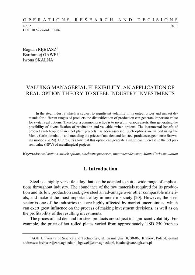
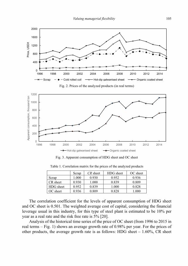
The data used in the analysis are presented in Figs. 23 and Table 1. Figure 2 shows the prices (in real terms) of CR sheet, HDG sheet, OC sheet and scrap. Figure 3 shows the apparent consumption of HDG sheet and OC sheet. Table 1 presents the correlation matrix for the prices of the analyzed products.
Valuing managerial flexibility
105
Fig. 2. Prices of the analyzed products (in real terms)
Fig. 3. Apparent consumption of HDG sheet and OC sheet
Table 1. Correlation matrix for the prices of the analyzed products
The correlation coefficient for the levels of apparent consumption of HDG sheet
and OC sheet is 0.501. The weighted average cost of capital, considering the financial leverage usual in this industry, for this type of steel plant is estimated to be 10% per year as a real rate and the risk free rate is 5% [20].
Analysis of the historical time series of the price of OC sheet (from 1996 to 2015 in real terms – Fig. 1) shows an average growth rate of 0.98% per year. For the prices of other products, the average growth rate is as follows: HDG sheet – 1.60%, CR sheet
– 1.86%, scrap – 1.74%. Based on this, we estimate an annual price growth rate of 1.5% in common for all of the products, as it is assumed that this increase was partly a result of the structural changes which occurred in the sector during the economic boom, which occurred in 2006–2007.
Analysis of the historical series of the apparent consumption of OC sheet and HDG sheet (from 1996 to 2015, Fig. 2) shows an average growth rate of 8.00% per year for HDG sheet and 9.23% for OC sheet. Based on this, we use 7.00% as the annual increase in demand for all products, as it is assumed (as above) that this increase was partly a result of the structural changes which occurred in the sector during the economic boom, which occurred in 2006–2007.
The volatility parameter was estimated by the standard deviation of the log return of the price series and demand series shown, respectively, in Figs. 1 and 2 according to Eqs. (10)(12). These values are equal to:
for prices: scrap 16.37%, CR sheet 21.09%, HDG sheet 19.92%, OC sheet 13.70%; for apparent consumption: HDG sheet 11.97%, OC sheet 16.64%. The other variable production costs (energy, manpower and maintenance) amount to
approximately USD 114.0 per ton of HDG sheet and USD 174.0 per ton of OC sheet. The fixed costs for a HDG sheet plant are estimated as USD 31.08 million per year. The incre-mental fixed costs for an OC sheet plant are estimated as USD 12.95 million per year. The initial investment for an OC sheet plant amounts to approximately USD 40 million. The market share for HDG sheet was estimated to be 30% and for OC sheet to be 25%.
Using the methodology described above (Eq. (19)), the premiums () were esti-mated as follows:
for prices: scrap 0.81%, CR sheet 0.79%, HDG sheet 1.01%, OC sheet 0.75%; for apparent consumption: HDG sheet 1.32%, OC sheet 2.11%. On the basis of these assumptions, the simulations were realized and the static NPV
and the value of a product switch option for the project were calculated.
Valuing managerial flexibility
107
4.3. Results and discussion
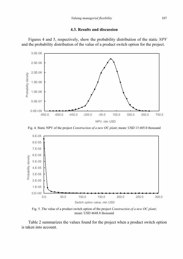
Figures 4 and 5, respectively, show the probability distribution of the static NPV and the probability distribution of the value of a product switch option for the project.
Fig. 4. Static NPV of the project Construction of a new OC plant; mean: USD 13 605.0 thousand
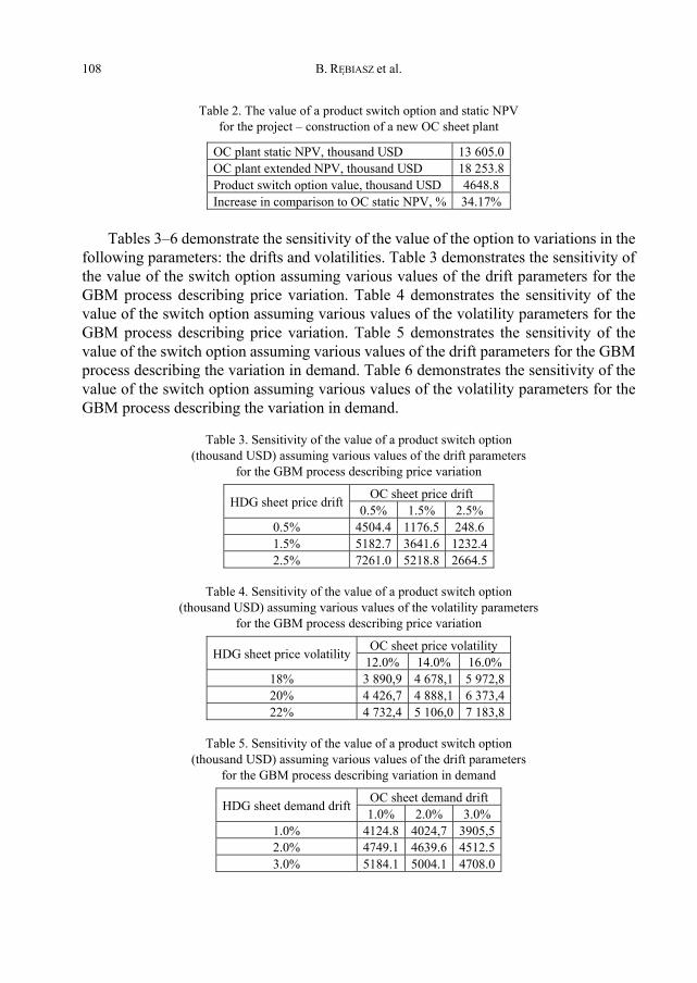
Fig. 5. The value of a product switch option of the project Construction of a new OC plant;
mean: USD 4648.8 thousand
Table 2 summarizes the values found for the project when a product switch option is taken into account.
Tables 3–6 demonstrate the sensitivity of the value of the option to variations in the
following parameters: the drifts and volatilities. Table 3 demonstrates the sensitivity of the value of the switch option assuming various values of the drift parameters for the GBM process describing price variation. Table 4 demonstrates the sensitivity of the value of the switch option assuming various values of the volatility parameters for the GBM process describing price variation. Table 5 demonstrates the sensitivity of the value of the switch option assuming various values of the drift parameters for the GBM process describing the variation in demand. Table 6 demonstrates the sensitivity of the value of the switch option assuming various values of the volatility parameters for the GBM process describing the variation in demand.
Table 3. Sensitivity of the value of a product switch option (thousand USD) assuming various values of the drift parameters
As can be seen in Table 2, assuming that the prices of the analyzed products follow
GBM, the value of a product switch option represents 34.17% of the static NPV. In Tables 3 and 5, it can be observed that the value of a product switch option increases as the drift of the price of and demand for HDG sheet increases relative to the drift of the price of and demand for OC sheets.
Tables 4 and 6 show that the value of the switch option increases as the volatility of the prices of and demand for the analyzed products increases.
The sensitivity analysis shows that product switch options have a significant rele-vance to the evaluation of a project in the steel industry for a wide range of values of the parameters describing the underlying stochastic processes.
5. Conclusions
Investment decisions in industrial plants are taken in an uncertain environment, where the variability of prices and the quantities demanded have the capacity to signif-icantly affect the economic performance of projects.
The proposed model of a product switch option was tested on a hypothetical exam-ple, which is similar to many real case studies in the metallurgical industry and the ex-perimental results verify the rationality and effectiveness of the method.
This paper estimated the projected cash flows, which are dependent on fluctuations in demand and prices, and calculated the value of the option available to this industry of delivering the product that maximizes revenue in each future period. Using a GBM approach, the authors concluded that this option significantly increases the NPV of an OC sheet production plant and considerably enhances the value created by metallurgical projects for shareholders.
Furthermore, it is possible to observe that the value of the product switch option increases when the drift of the price of and demand for HDG plate is greater than the drift of the price of and demand for OC plates and as the volatility of demand and prices increases. The sensitivity analysis shows that product switch options have a significant relevance to the evaluation of a project in the metallurgical industry for a wide range of values of the parameters describing the underlying stochastic processes.
B. RĘBIASZ et al.
110
References
[1] BASTIAN-PINTO C., BRANDÃO T., HAHN W.J., Flexibility as a source of value in the production of al-ternative fuels. The ethanol case, Energy Economics, 2009, 31 (3), 411–422.
[2] BASTIAN-PINTO C., EDUARDO L., BRANDÃO T., RAPHAEL R., OZORIO L.M., Financial Valuation of Op-erational Flexibilities in the Aluminum Industry Using Real Option Theory, [in:] Proc. 17th Annual International Conference Real Options: Theory Meets Practice, Tokyo 2013, 1–23.
[3] BJERKSUND P., EKERN S., Managing investment opportunities under price uncertainty. From last chance to wait and see strategies, Fin. Manage., 1990, 19 (3), 65–83.
[4] BLANK F.F., BAYDIA T.K.N., DIAS M.A., Private infrastructure investment through public private partnership. An application to a toll road highway concession in Brazil, 13th Annual International Conference on Real Options, Braga, Portugal, Santiago, Spain, 2009, 1–21.
[6] BYKO M., TMS Plenary Symposium. Energy Reduction in the Aluminum Industry, J. Miner., Met. Mater. Soc., 2002, 54 (5), 39–40.
[7] DAS S., LONG W., HAYDEN H., GREEN J., HUNT W., Energy implications of the changing world of alu-minum metal supply, J. Miner., Met. Mater. Soc., 2004, 56 (8), 14–17.
[8] DESSUREAULT S., KAZAKIDIS V.N., MAYER Z., Flexibility valuation in operating mine decisions using real options pricing, Int. J. Risk As. Manage., 2007, 7 (5), 656–674.
[9] DIMITRAKOPOULOS R., SABOUR S.A.A., Evaluating mine plans under uncertainty. Can the real options make a difference?, Res. Pol., 2007, 32 (3), 116–125.
[10] DIXIT A.K., PINDYCK R.S., Investment under Uncertainty, Princeton University Press, 1994. [11] DULEY B.D.L.J., JOHNSON B.E., As Good as It Gets. Optimal Fab Design and Deployment, IEEE
investment based on fuzzy-interval grey system theory and geometric Brownian motion, J. Appl. Math., 2014, article ID 914643, 1–12.
[13] HERBELOT O., Option valuation of flexible investments. the case of environmental investments in the electric power industry, Department of Nuclear Engineering Massachusetts Institute of Technology, 1992 (https://dspace.mit.edu/bitstream/handle/1721.1/50208/35720932.pdf?sequence = 1).
[14] HULL J.C., Options, futures and other derivatives securities, 6th Ed., Prentice Hall, Englewood Cliffs 2006.
[15] IRWIN T., Public Money for Private Infrastructure. Deciding When to Offer Guarantees, Output-Based Subsidies, and Other Fiscal Support, World Bank Working Paper, 2003 (https://openknowledge. worldbank.org/handle/10986/15117 License: CC BY 3.0 IGO).
[16] MARATHE R., RYAN S.M., On the validity of the geometric Brownian motion assumption, Eng. Econ., 2005, 50 (2), 1–40.
[17] MOREIRA A., ROCHA K., DAVID P., Thermopower generation investment in Brazil. Economic condi-tions, En. Policy, 2004, 32 (1), 91–100.
[18] MUHARAM F.M., Assessing risk for strategy formulation in steel industry through real options analy-sis, J. Global Strat. Manage., 2011, 5 (2), 5–15.
[19] MYERS S., Determinants of corporate borrowing, J. Fin. Econ., 1977, 5 (2), 147–175. [20] OZORIO L.M., BASTIAN-PINTO C., BAIDYA T.K.N., BRANDÃO T., Investment decision in integrated steel
plants under uncertainty, Int. Rev. Fin. Anal., 2013, 27 (3), 55–64. [21] PINDYCK R.S., RUBINFELD D., Econometric Models and Economic Forecasts, McGraw-Hill, 1998. [22] REBIASZ B., Polish steel consumption 1974–2008, Res. Pol., 2006, 31 (1), 37–49. [23] RUEY S.T., Analysis of Financial Time Series, Wiley, New York 2002.
Valuing managerial flexibility
111
[24] SAMIS M., DAVIS G.A., Using Monte Carlo simulation with DCF and real options risk pricing tech-niques to analyse a mine financing proposal, Int. J. Fin. Eng. Risk Manage., 2014, 1 (3), 264–281.
[25] SLADE M., Valuing managerial flexibility. An application of real-option theory to mining investments, J. Environ. Econ. Manage., 2001, 41 (2), 193–233.
[26] WATTANARAT V., PHIMPHAVONG P., MATSUMARU M., Demand and Price Forecasting Models for Stra-tegic and Planning Decisions in a Supply Chain, Proc. of the School of Science of Tokai University, 2010, 3 (2), 37–42.
[27] WILIMOWSKA Z., ŁUKANIUK M., Binomial model of valuation of property options, Bad. Oper. Dec., 2005 (1), 71–83 (in Polish).