University of Oxford Kellogg College Master of Science in Mathematical Finance Valuing power plants under emission reduction regulations and investing in new technologies: An exchange option on real options d-fine GmbH 1 Supervisor: Professor Sam Howison 2 April 2010 1 d-fine GmbH, Opernplatz 2, 60313 Frankfurt, Germany (info@d-fine.de) 2 University of Oxford, Mathematical Institute, [email protected]
Transcript
University of Oxford
Kellogg College
Master of Science in Mathematical Finance
Valuing power plants under emissionreduction regulations and investing in newtechnologies: An exchange option on real
options
d-fine GmbH1
Supervisor: Professor Sam Howison2
April 2010
1d-fine GmbH, Opernplatz 2, 60313 Frankfurt, Germany ([email protected])2University of Oxford, Mathematical Institute, [email protected]
Abstract
In this dissertation we model the value of a power generation asset through areal option approach. With electricity, fuel and emission allowances we expressevery essential uncertainty on the energy market by an own stochastic process andderive an optimal clean spark spread. Typical operational constraints of a powerplant are taken into account. Beside analysing the behaviour of the generationasset under different constraints, we want to evaluate the option to invest in newtechnologies to improve these constraints. In this dissertation, we do not set upthe standard American option with strike equal to the investment as usual, butset up an exchange option on two real options with different constraints. We showthat this approach handles an option on new technology much more sensitive tothe individual price uncertainties and considers all possible employments. If theintrinsic value of the exchange option exceeds the realization costs, it is time toinvest. We also state an explicit Monte Carlo algorithm and present numericalresults for the option to install a Carbon Capture and Storage unit.
The world demand for energy is constantly rising. Nowadays, especially for newemerging economies like India, China and Brazil, energy is the basis for economicgrowth and wealth. In contrast, it is well known that the fossil energy sourceson earth are limited and the accessible coal stocks, oil and gas sources will lastfor few more decades only. Additionally, pollution and global climate changebecomes a big issue around the world with the power industry as the biggest pol-luter. Do these aspects put fuel-fired power plants to the stack of old technologies?
A first argument against this hypothesis is, that by 2015 a generation of nuclearpower plants in European nations will have to be shut down because they arebecoming old and unsafe3 and no new ones could be build well-timed for yearsafter that4. Secondly, alternative resources like Uranium will last for 83 years atthe current rate of consumption5. This is shorter than other fossil energy resourcelike coal with its current reserves-to-production ratio of 137 years according toIEO20096. Thirdly, renewables are not reliable and even the latest technology im-provements are far away from generating the needed huge amount of electricity.And last but not least, there are several technology improvements in efficiency,flexibility and emission reduction for coal and gas power plants. Thus, the majorpart of electricity produced worldwide currently comes and will come from fuel-driven power plants for the next decades, which makes them a desirable object forinvestors. For example, in the IEO2009 reference case, world coal consumptionincreases by 49% from 2006 to 2030.
For an investment in existing or new physical assets it is necessary to evaluatethe proper value of the object. In this thesis we want to estimate the value offuel driven power plants as electricity generation assets which consuming fuel andproducing emissions. We do this by simulating electricity, fuel and emission al-lowances as uncertainties on the energy market, each through a selected stochasticprocess and derive the so called clean spark spread, the margin between these threecommodities.
For valuation we use a real option approach. An alternative and common methodis called Discounted Cash Flows (DCF) which sums the expected, discountedfuture cash flows to estimate the present value. There are three mainly disadvan-
3ARD, www.tagesschau.de/inland/meldung1516.html Standorte und Laufzeiten deutscherAtomkraftwerke, 2004
4The Economist, How long till the lights go out?, Aug 6th 20095International Atomic Energy Agency, Nuclear Technology Report 2009, 20096Energy Information Administration, International Energy Outlook 2009, May 2009
3
tages of the DCF method. Firstly, the estimated value of the cash flows may bedifficult to assess for distant years. Secondly, it is difficult to assess right discountfactors including the risk aversion of investors and thirdly, it does not includetechnical properties of the facility or operational irregularity. For more details onDCF and its merits and limits see for example [Geman05]. Differently to DCF,the real option approach can captures typical operational constraints of a powerplant. Also the operational, irreversible decisions a plant operator will have madeare considered by setting the asset to different states. One more advantage ofa real option approach is, that it captures the impact of price volatility to thevalue of a power plant more realistically. Keeping in mind that a modern peaker- a very flexible generation unit - has very high ramp rates, the operator has theoption to adjust production over very short time periods to face price movementsin a volatile market. Surely, a real option approach also has its difficulties. Anappropriate stochastic process can be measured only if there are liquid markets.We will come back to this issue in section 4.2.
One special goal in this dissertation is to introduce the additional uncertaintyemission allowance prices into the clean spark spread by a separate stochasticprocess and observe its affect to power plant values. Our motivation is that cli-mate change due to industry emission has become a severe political issue becauseit affects the environment of the whole planet and is thought to be responsible fornatural disasters. There are new regulations from advisors to meet their promisesto reduce emission made in the Kyoto Protocol. The Kyoto protocol takes careof six different greenhouse gases: carbon dioxide CO2, methane CH4, nitrous ox-ide N2O, sulphur hexafluoride SF6, hydrofluorocarbons H − FKW/HFCs andperfluorocarbons FKW/PFCs. On the one hand, emissions of most of thesegases are allowed under restrictions and taxation and the costs per emitted unitis rather deterministic. Thus we will capture these costs in the deterministic op-erational and maintaining costs. One the other hand, CO2 is part of the Kyotoemissions trading flexible mechanism and thus emission allowance prices dependon supply and demand. In the European Union, a very important instrument isthe European Union Emission Trading Scheme (EU-ETS) where CO2 emissionallowances can be traded between emission producers and emission reducers orother counterparties. Here we focus on this market. A short introduction to theEU-ETS is given in the Appendix.
Furthermore, we want to evaluate the option to invest into emission reductiontechnologies like a Carbon Capture and Storage (CCS) unit. Small pilot plantshave been built with these new technologies but nobody knows whether or whenit will be needed to install CCS in big projects. To handle this issue we do not
4
follow former articles on this topic which go from the costs point of view andtry to identify building costs and average savings and model an American option.We come from the profit point of view and use our real option model to valuethe actual returns including the new technology. This approach handles a newtechnology much more sensitive and consider all its possible employments thanstandard American options. In fact, a technology investment is originally nothingelse than an exchange of operational parameters and thus can be modelled as anexchange option on two real options with different constraints.
The thesis is organised as follows: we start by setting up the model to value ageneral fuel-driven generation asset. The clean spark spread is defined and for alluncertainties proper stochastic processes are identified. Then, in section 2.3 weintroduce the treatment of a number of general constraints on generation assets,which leads us to a complex multi-state problem. In section 3 we explain thereal option approach to model this multi-state problem. To solve it the dynamicprogramming technique is introduced in section 3.2 Then, we use Least SquareMonte Carlo methods firstly introduced by Longstaff and Schwartz to find a so-lution. Numerical and implementation aspects are showed in section 4 and someanalyses on assets with typical constraints are illustrated together. Going one stepfurther, section 5 describes the valuation of an investment option on technologicalimprovements or upgrades that influence model parameters. According to thisAmerican style option, price and volatility boundaries are identified to catch theoptimal exercise time. We close the discussion by giving an outlook of furtheranalysis and investigations.7
7Special thanks to Tilman Huhne and Yuri Ivanov for their useful comments.
5
2 Modelling power plants
In the following section we will set up a model to value a general fuel fired powerplant including its operational constraints.
2.1 The clean spark spread
A fuel-fired power plant converts a particular fuel like coal, gas or biomass intoelectricity. This conversion involves at least two marketed commodities, fuel andelectricity. Thus, the value of a fuel fired power plant V strongly depends on the socalled spark spread Π, defined as the difference between the marked price of elec-tricity PE (US$/MWh) and the price of gas, coal or biomass P F (US$/mmBtu)used for the generation of electricity. It also depends on the two prices individ-ually because a power plant needs starting fuel or consumes electricity by itself.We will come back to these issues in section 2.3. In this thesis, the amount ofnatural gas is measured in million British Thermal Units (mmBtu). The standardunit for coal or biomass is tonne but can be converted easily to mmBtu. For ex-ample, one tonne of anthracite coal is equivalent to 25.09 mBtu8. Sometimes, inliterature the spark spread for a coal fired power plant is called dark spark spread.
The first proposals for this valuation approach came from Hsu [Hsu98] and Deng,Johnson and Sogomonian [Deng98], who modelled the payoff of a generator as thespark spread:
Π = PE −HRPF (1)
where HR (mmBtu/MWh) denotes the heat rate, the amount of fuel burned toproduce 1 unit of electricity. In their approach, the value of a power plant V is thesum of European style options with this spark spread as payoff for every 1 MWhelectricity generation. An extension to this model includes the costs for emissionproduced by burning fuel according to the EU-ETS. It is called the clean sparkspread and defined as:
Πc = PE −HRPF − ERPA (2)
where PA (US$/tonne CO2) stands for the allowance price to emit one tonne ofcarbon dioxide and ER (tonnes CO2/MWh) is the number of tonnes of carbondioxide emitted by production of 1 MWh of electricity. If we define q (MW) asthe generation level of the power plant - power output or energy generated per
8A energy units conversion table can be found at: http://www.energystar.gov/ia/business/tools resources/target finder/help/Energy Units Conversion Table.htm
6
time - and redefine HR = HR(q) (mmBtu/h) and ER = ER(q) (tonnes CO2/h)accordingly, the clean spark spread Πc(q) of the power plant is
Πc(q) = qPE −HR(q)P F − ER(q)PA. (3)
For the purpose of maximizing profit, a power plant operator will switch gener-ation on whenever it is profitable to do so, i.e. when at time t the clean sparkspread Πc
t(qt) exceeds the operational costs OMt (US$/h). Assuming a very shortswitching time, fast notice of price movements and deterministic interest rates,we can state that the value of the generation asset at time t0 is
Vt0 =
tN∑t=t0
D(t0, t)Et0 [∆tmax (Πct(qt)−OMt, 0) |Ft0 ] (4)
where the number N depends on the granularity ∆t = ti+1 − ti for all i = 0...Nand the plant’s lifetime T = tN . For practical applications, the granularity shouldcomply with the operational precision of the generator. Here D(t0, t) stands forthe discount factor from t0 to t and Et0 stands for the expectation at time t0 underan appropriate filtration Ft0 . A filtration is an increasing sequence of σ-algebrasFtt≥t0 on a measurable space Ω. Here Ω is the probability space for price move-ments with the risk neutral measure Q. In (4) we used the principle of efficientand complete markets without arbitrage where a Q-Martingale exists under therisk neutral measure Q. For more details on probability spaces, filtrations and riskneutral measures in arbitrage free financial markets see for example [Hull02]. Wenotice that (4) is equal to the value of a strip of standard European style spreadoptions.
In literature there exist many models to describe price uncertainties with stochas-tic processes that are trying to catch observable market behaviour. Before we willextend our model to real options by considering operational constraints, we wantto discuss the behaviour of the three price uncertainties.
2.2 Energy markets
2.2.1 Electricity prices
Electricity is one of the most exotic commodity due to its lack of efficient stora-bility. We have to keep in mind that power itself is not a tradable asset, i.e. spotpower can be sold during a price spike but it cannot be borrowed, shorted, andthen bought back and returned several days later. Thus, intertemporal conceptslike efficient markets for asset pricing do not apply to power spot dynamics. Nev-ertheless, efficient markets still can be applied to the pricing of derivatives on
7
power and we will use observable market values for spot hourly auction prices inorder to calibrate implied model parameters. For more details on this topic see[Seppi02].
0
10
20
30
40
50
60
70
80
15
.09
. 0
0-0
1
12
-13
16
.09
. 0
0-0
1
12
-13
17
.09
. 0
0-0
1
12
-13
18
.09
. 0
0-0
1
12
-13
19
.09
. 0
0-0
1
12
-13
20
.09
. 0
0-0
1
12
-13
21
.09
. 0
0-0
1
12
-13
Time
€/MWh
0
5.000
10.000
15.000
20.000
25.000
MWh
Price
Volume
Figure 1: Spot Hourly Auction prices at the European Energy Exchange, Phelix,from Tue. 15th Sep. 2009 to Mon. 21st Sep. 2009
Regarding liquid markets like the European Energy Exchange EEX in Fig. 19,we can observe some special behaviour of electricity spot prices. First, there is ahourly structure in the price level that reflects the average schedule of private andindustrial consumers. Market participants distinguish these hourly periods intothe following so called Blocks: Offpeak, Off Peak I, Off Peak II, Night, Morning,High Noon, Afternoon, Rush Hour, Evening and Business Hours. Second there isa difference between working days and weekends or bank holidays on total demandand price levels consequently. Third, on the intraday spot market we can observeprice spikes emerging when demand exceeds the current supply, i.e. when a baseload plant in the power grid has an unscheduled forced outage.
For our purpose to value a power plant as an option to produce electricity only ifit is profitable, according to the constraints given in section 2.3, we explicitly take
9source: www.eex.com
8
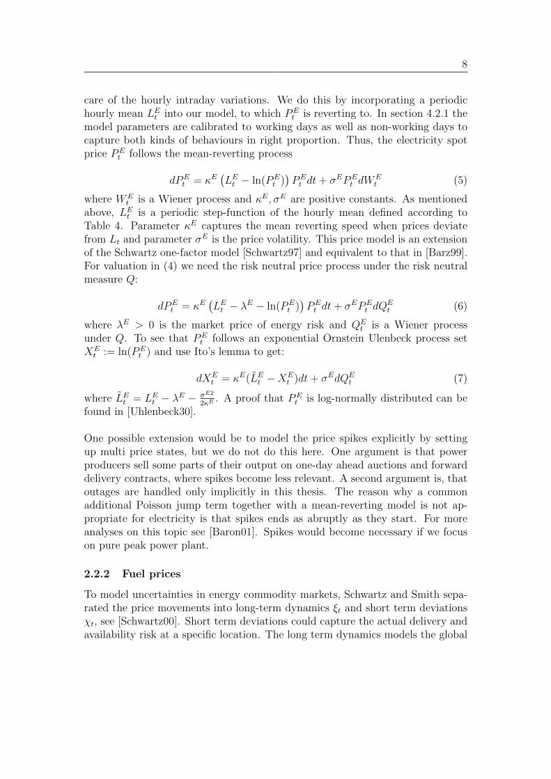
care of the hourly intraday variations. We do this by incorporating a periodichourly mean LEt into our model, to which PE
t is reverting to. In section 4.2.1 themodel parameters are calibrated to working days as well as non-working days tocapture both kinds of behaviours in right proportion. Thus, the electricity spotprice PE
t follows the mean-reverting process
dPEt = κE
(LEt − ln(PE
t ))PEt dt+ σEPE
t dWEt (5)
where WEt is a Wiener process and κE, σE are positive constants. As mentioned
above, LEt is a periodic step-function of the hourly mean defined according toTable 4. Parameter κE captures the mean reverting speed when prices deviatefrom Lt and parameter σE is the price volatility. This price model is an extensionof the Schwartz one-factor model [Schwartz97] and equivalent to that in [Barz99].For valuation in (4) we need the risk neutral price process under the risk neutralmeasure Q:
dPEt = κE
(LEt − λE − ln(PE
t ))PEt dt+ σEPE
t dQEt (6)
where λE > 0 is the market price of energy risk and QEt is a Wiener process
under Q. To see that PEt follows an exponential Ornstein Ulenbeck process set
XEt := ln(PE
t ) and use Ito’s lemma to get:
dXEt = κE(LEt −XE
t )dt+ σEdQEt (7)
where LEt = LEt − λE − σE2
2κE. A proof that PE
t is log-normally distributed can befound in [Uhlenbeck30].
One possible extension would be to model the price spikes explicitly by settingup multi price states, but we do not do this here. One argument is that powerproducers sell some parts of their output on one-day ahead auctions and forwarddelivery contracts, where spikes become less relevant. A second argument is, thatoutages are handled only implicitly in this thesis. The reason why a commonadditional Poisson jump term together with a mean-reverting model is not ap-propriate for electricity is that spikes ends as abruptly as they start. For moreanalyses on this topic see [Baron01]. Spikes would become necessary if we focuson pure peak power plant.
2.2.2 Fuel prices
To model uncertainties in energy commodity markets, Schwartz and Smith sepa-rated the price movements into long-term dynamics ξt and short term deviationsχt, see [Schwartz00]. Short term deviations could capture the actual delivery andavailability risk at a specific location. The long term dynamics models the global
9
long term demand and supply risk of exhausting resources. A third aspect is theweather. Besides the usage as fuel gas in power plants, natural gas is neededin cold winters to heat homes, offices and facilities. The additional demand in-creases prices during these periods. If we consider the pure spark spread withoutany constraints and look at period of years we could average these effects out.But later we will introduce constraints and we also take a look at timescales ofa few month. Thus we model the additional demand with a seasonal factor s(t).All three aspects are observable in the current market Futures illustrated in Fig.210.
3
4
5
6
7
8
9
Ju
l. 0
9
Ju
l. 1
0
Ju
l. 1
1
Ju
l. 1
2
Ju
l. 1
3
Ju
l. 1
4
Ju
l. 1
5
Ju
l. 1
6
Ju
l. 1
7
Time
$/mmBtu
Figure 2: Natural Gas Future prices with monthly delivery for different maturitiesat New York Mercantile Exchange, Henry Hub, on 14th Sep. 2009
Putting everything together, we assume the following 2-factor Schwartz-Smithprocess with seasonality for fuel spot price P F
t at time t:
P Ft = eχt+ξts(t) (8)
where
10source: Reuters
10
dχt = −κχtdt+ σχdW χt
dξt = µdt+ σξdW ξt
dW χt dW
ξt = ρχξdt
(9)
and
s(t) :=12∑i=1
θi(t)
[γi + (γi+1 − γi)
t− titi+1 − ti
]. (10)
Here W χt and W ξ
t are two Wiener processes with correlation ρχξ. κ > 0 is thereverting speed of χt to zero, µ > 0 is the drift of ξt and σχ, σξ > 0 measuring bothrisks accordingly. In the seasonality function s(t), γi > 0 are the monthly seasonalfactors normalized to 1 by the constraint 1
12
∑12i=1 γi = 1 and θi(t) represents the
characteristic indicator function:
θi(t) :=
1 if t ∈ [ti, ti+1]0 otherwise.
(11)
Thus s(t) is a periodic function defined through linear interpolation between the12 seasonal factors γi, see Figure 3.
0 1 2 30.9
0.95
1
1.05
1.1
time (years)
se
aso
na
l fa
cto
r
Figure 3: A normalized seasonality curve s(t) with γi estimated from market dataJanuary 2010.
11
Because Natural Gas is traded in monthly contract, 12 is the maximum numberof seasonal factors one can estimate out of market data at once. In literatureit is quite common to model the seasonality by an additive term like s(t) =∑S
i=1 bEi sin(2πit
P) + cEi cos(
2πitP
). In one of our last module hand in [Ludwig09]we showed that constant seasonal factors are much more applicable and easierto calibrate to market data than additive trigonometric functions. The reason isthat the market amplitudes of seasonal oscillations are proportional to the futureprices, see Figure 2. Especially they are not constant as an additive term wouldsuggest. This is the reason why we multiply prices with the seasonal factor s(t)here. As in the previous section, for option valuation we define the risk-neutralprocess
dχt = (−λχ − κχt)dt+ σχdQχt
dξt = (µ− λξ)dt+ σξdQξt
(12)
where λχ, λξ > 0 and Qχt , Q
χt are Wiener processes under the risk-neutral measure
Q. For the log-price XFt = ln(P F
t ) we get the following evolution equation:
dXFt = (µ− λχ − κχt)dt+ σχdQχ
t + σξdQξt + ln(s(t)) (13)
where µ = µ− λξ.
2.2.3 Emission allowance prices
The European Union Emission Trading Scheme (EU-ETS) is a system wherebyCO2 emission allowances are traded among the market participants and thus varywith the level of demand. For the power plant valuation, we want to find an appro-priate price process to model this uncertainty. At the present time, one problemto find a stochastic process with stable parameters is the frequent changes of theEU-ETS by regulators. As mentioned above, the Member States set up their ownNational Allocation Plan (NAP) and choose the industry sectors that have to par-ticipate nationwide. Great Britain for example, add a big amount of allocationsto their NAP after the trial period (2005-2007) already started which caused abig price drop throughout the European Union. Later, at the beginning of thesecond period (2008-2012), there were more changes like the convertibility to theKyoto Certified Emission Reduction units (CER) and for the beginning of thethird period, 2013, more changes are constituted already, see section 6. A secondproblem is, that at least 95% of allowances were free of charge in the fist trialperiod. This fact prevented a strong exchange and thus the development of a veryliquid market. Bigger nations like Germany even allocated 100% of allowances for
12
this period free of charge11. A change away from these free allocations towardsmore auctions will continue in 2013. Thirdly, emitters have to deliver the neededamount of allowances at the end of each year and not at the time of emission.Furthermore, holders can transfer unused allowances to the next year within thesame period, but not across the border of different periods. Both facts can sup-port the occurrence of strong price movements or even jumps.
In literature, we found different approaches to model this uncertainty emissionallowance prices. For example, Abadie and Chamorro [Chamorro08] observed themarket behaviour of European emission allowance future contracts over a periodof one year. With 1,325 daily observations for 5 futures contracts maturing fromDec-08 to Dec-12 they figured out that the behaviour of prices is hardly con-sistent with a mean reversion process. Truck [Trueck08] analysed GARCH andRegime-switching models and conclude that: ’the best example fit to the data isprovided by a regime-switching model with an autoregressive process in the baseregime and a normal distribution for the spike regime. Results for the GARCHand normal mixture regime-switching models are only slightly worse’. Daskalakis[Daskal05] suggests that CO2 emission allowance price levels are non-stationaryand exhibit abrupt discontinuous shifts. For logarithmic returns they find thatthe distribution is clearly non-normal and characterized by heavy tails. Theyfurther find that the best model fits for allowance prices in terms of likelihoodis obtained by a geometric Brownian motion with an additional jump-diffusioncomponent. ’This model is also able to produce the discontinuous shifts in theunderlying diffusion that are observed in the CO2 emission allowances prices’. Ananalysis at a big European bank - name is confidential - give us the insight that’the jumps’ - of a Merton jump-diffusion model - ’seem to be a key ingredientin the CO2 modelling’. Some compared GARCH models fit quite good also, butrequire more parameters to estimate and thus loose robustness.
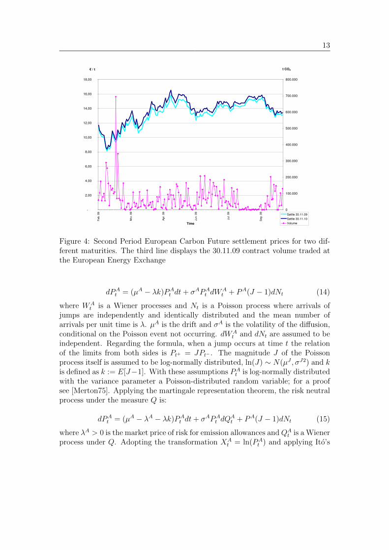
Considering the market behaviour - the structure of demand and supply and thearrival of important new information as described above - the presence of jumps isreasonable. Regarding Fig. 4, it is also reasonable to expect that beside the timeswhen such information arrives, there will be ”quiet” times as Merton describedin his paper [Merton75]. In addition, the historical returns in the bank analysisshow fat tails and some negative skewness that could corresponds to the presenceof jumps with negative jump mean. Thus, in this thesis we will apply the jump-diffusion model proposed by Merton to model the price of the allowance to emit1 tonne of CO2 at time t:
11Federal Ministry for the Environment, Nature Conservation and Nuclear Safety, NationalAllocation Plan for the Federal Republic of Germany, March 2004
13
-
2,00
4,00
6,00
8,00
10,00
12,00
14,00
16,00
18,00
Feb. 09
Mrz
. 09
Apr.
09
Jun. 09
Jul. 0
9
Sep. 09
Time
€ / t
0
100.000
200.000
300.000
400.000
500.000
600.000
700.000
800.000
t CO2
Settle 30.11.09
Settle 30.11.10
Volume
Figure 4: Second Period European Carbon Future settlement prices for two dif-ferent maturities. The third line displays the 30.11.09 contract volume traded atthe European Energy Exchange
dPAt = (µA − λk)PA
t dt+ σAPAt dW
At + PA(J − 1)dNt (14)
where WAt is a Wiener processes and Nt is a Poisson process where arrivals of
jumps are independently and identically distributed and the mean number ofarrivals per unit time is λ. µA is the drift and σA is the volatility of the diffusion,conditional on the Poisson event not occurring. dWA
t and dNt are assumed to beindependent. Regarding the formula, when a jump occurs at time t the relationof the limits from both sides is Pt+ = JPt− . The magnitude J of the Poissonprocess itself is assumed to be log-normally distributed, ln(J) ∼ N(µJ , σJ2) and kis defined as k := E[J−1]. With these assumptions PA
t is log-normally distributedwith the variance parameter a Poisson-distributed random variable; for a proofsee [Merton75]. Applying the martingale representation theorem, the risk neutralprocess under the measure Q is:
dPAt = (µA − λA − λk)PA
t dt+ σAPAt dQ
At + PA(J − 1)dNt (15)
where λA > 0 is the market price of risk for emission allowances andQAt is a Wiener
process under Q. Adopting the transformation XAt = ln(PA
t ) and applying Ito’s
14
Lemma12 yields:
dXAt = µAdt+ σAdQA
t +
Nt+dt∑i=Nt
ln(Ji) (16)
= µAdt+ σAdQAt + ln(J)dNt. (17)
where µA = µA − λA − λk − σA2
2.
2.2.4 Correlations
From the nature of things it is clear that electricity prices, fuel prices and emissionallowance prices are not independent and their processes that are responsible forprice development are correlated. The correlations between the four stochasticprocesses are:
Thus far we defined the Clean Spark Spread for a fuel fired power plant as a stripof European style spread options the operator holds. But a power plant can’t beswitched on and off immediately whenever it is profitable to do so. There areseveral constraints on the operating states transforming the operator’s decisionpossibilities into real options. Les Clewlow and Chris Strickland [Clewlow09],Chung-Li Tseng [Tseng09] or Graydon Barz [Barz02], for example, introducedmethods to model complex operational constraints. The following list summarizesoperational constraints that can be found in literature applied on spark spreadsand power plant valuation approaches. The text in parenthesis indicates if theconstraint is handled in this dissertation or not:
12Using the generalised Ito formula for semi-martingales; proof see e.g. [Duevel01]
15
• minimum stable generation (yes)• ramp-up rates (yes)• ramp-down rate (yes)• minimum up time (yes)• minimum down time (yes)• cold time (yes)• start-up costs (yes)• shut-down costs (yes)• variable operational and maintenance cost (yes)• self used electricity (yes)• forced outages (no)• scheduled maintenance (no)• over fireing (no)• outside temperature (no)• fuel transportation costs (no)• power transmission costs (no)
Before we discuss every constraint in detail, we want to recall the time discreti-sation into N time intervals with ti ∈ [t0, T ] for all i = 1...N where tN = T is theremaining lifetime of the power plant and ∆t = ti+1 − ti is constant.
2.3.1 Heat rate, emission rate and optimal generation level
We already introduced the power plant generation level qt in section 2.1. Thecapacity qmax is the maximum generation level of the plant, qmin the level of min-imum stable generation and qt ∈ [qmin, qmax]. Once the generator is producingelectricity at time t, the operator can switch qt to any level within [qmin, qmax].That means qt is a real time decision process and does not restrict any furtherdecisions.
As is standard, the heat rate HR is modelled as a quadratic function of the gen-eration level qt. For arguments on this assumption see [Wood84]. We define:
HR(qt) = a0 + a1qt + a2q2t (19)
where a0, a1, a2 > 0 are positive constants. A chemical engineer at Didcot13
provides us with the information that the emission rate has a constant proportionto the fuel burned, no matter which temperature or pressure exists in the reactor.So we define the emission rate ER at time t to be:
13The RWE npower site at Didcot UK is host to two power stations - 2000MW dual-fired coalstation and the 1360 MW combined cycle gas turbine station.
16
ER(qt) = qt · E (20)
where E > 0 (tonnes CO2/MWh) is the constant emission quotient specifyinghow many tonnes of CO2 are emitted by producing one MWh of electricity.
The dispatch problem of the power unit is to determine the optimal generationlevel q∗t at time t. Since the clean spark spread (3) is a convex quadratic functionof market prices observed at time t, q∗t can be calculated by maximizing:
Πc(qt) = qt · PEt −HR(qt)P
Ft + ER(qt)P
At
= qt(PEt − E · PA
t )− (a0 + a1qt + a2q2t )P
Ft .
(21)
We know that Π′(q) = (PE − E · PA) − (a1 + 2a2q)PF , set Π′(q) = 0 and note
that Π′′(q) < 0 always, to get q =(PE−E·PA
PF− a1
)1
2a2. So the optimal generation
level q∗t at time t is:
q∗t = min(qmax,max(qmin,
(PEt − E · PA
t
P Ft
− a1
)1
2a2
)). (22)
2.3.2 Ramp rates and start up costs
Most power plants cannot change their generation level instantaneously. A morerealistic dispatch algorithm has to consider ramp rates (MW/h) defined as therate at which the unit’s generation level q can increase or decrease in time. Nor-mally, ramp up rates can be classified as cold rc, warm rw or hot rh depending onhow long the unit has been off-line. The ramp down rate is equal to rh.
Given the unit is hot at time t already, assume that qmax−qminrh
< ∆t. The ramp
rates are captured in the calculation by defining the changing time τ =|q∗t−q∗t−1|
rhand adding the following penalty term to the operational costs:
Sh(t) = τ
[Πct(q∗t )− Πc
t(q∗t + q∗t−1
2)
]. (23)
We noticed that Sh(t) ≥ 0 always and Sh(t) = 0 if the plant operates on theoptimal level already. This is a quite good approximation neglecting the smallquadratic term of HR for the short time τ only. Moreover, the turbine channelof a generator can only be opened when a minimum level of pressure holds inthe connected steam-pipes. Otherwise the turbine would start to toggle. Thisimplies, that from a cold or a warm start the first fuel is burned only to heat thesteam-cycle and build up pressure in the pipes.
17
To capture this fact we define the time needed to reach the minimum stable gen-eration level tc,w = qmin
rc,wand assume that the time to reach the optimal generation
level tc,w + τ < ton. Here ton is the minimum up time defined in section 2.3.3. Thecost for the fuel burned and the CO2 emitted are:
St =(∫ tc,w
0HR(rc,wt)dt
)P Ft +
(∫ tc,w0
ER(rc,wt)dt)PAt
=(∫ tc,w
0a0 + a1rc,wt+ a2r
2c,wt
2dt)P Ft +
(∫ tc,w0
Erc,wtdt)PAt
=(a0tc,w + a1
2qmintc,w + a2
3q2mintc,w
)P Ft +
(E a1
2qmintc,w
)PAt
=[(a0 + a1
2qmin + a2
3q2min
)P Ft +
(E a1
2qmin
)PAt
]tc,w.
(24)
The complete start up costs Sc,w(t) include these fuel and emission costs St, theoptimal clean spark spread Πc
t(q∗t ) lost during this heat up time and the penalty
term Sh(t) to reach the optimal generation level:
Sc,w(t) = St + (Πct(q∗t )− Sh(t)) tc,w +
(Sminh (t+ tc,w)− Sh(t+ tc,w)
). (25)
Here, (Πct(q∗t )− Sh(t)) tc,w stands for a sum over discrete time intervals until tc,w
is reached. Sminh indicates that τmin =q∗t−qmin
rhis used instead of the original τ .
This is the reason why we add the difference Sminh (t+ tc,w)− Sh(t+ tc,w) here.Sometimes in literature these values are called switching cash flows, whish takecare of the fractional part of ∆t, i.e. 60 minutes, after the switch is completed.As an example, if the switch of qt takes 15 minutes, the switching cash flow isthe spark spread produced minus the optimal spark spread for these 15 minutes.After that, the plant is operating in the new optimal mode for the residuary 45minutes.
2.3.3 Minimum up time, minimum down time and cold time
The minimum time a unit must remain on after start up is called minimum uptime ton > 0. The minimum time the unit must remain off after shut down iscalled minimum down time toff > 0. During these periods no operating decisionscan be made. Furthermore, leaving the power plant off-line for a longer period,the reactor starts to cool down continuously. The time from shut down to thetime when the reactor reaches the surrounding temperature is called cold timetcold > toff > 0. We define the state variable:
xi ∈ X = −tcold, ...,−toff, ...,−1, 1, ..., ton (26)
which indicates the reactor state at time ti. After start up the state is increasingfrom 1 to ton, after shut down the state is decreasing from −1 to −toff or −tcold
18
probably. We notice that 0 is not a state. The future state xi+1 depends on theformer state xi and on the decision ui at time ti by the plants operator: ui = 0 forturning down and ui = 1 for turning up. Using these definitions, the constraintsfor minimum up time, minimum down time and cold time are:
xt+1(ut, xt) :=
min(ton,max(xt, 0) + 1) if ut = 1max(−toff,min(xt, 0)− 1) if ut = 0,
(27)
with the following possible decisions ui ∈ 0, 1 at time t:
ut(xt) :=
0 ∨ 1 if xt ∈ [−tcold,−toff]0 if − toff < xt ≤ −11 if 1 ≤ xt < tup0 ∨ 1 if xt = tup.
(28)
For a start-up from xi = −tcold the ramp rate is rc and for a start up from−tcold < xi ≤ −toff the ramp rate is rw. For later purpose, we define the set ofall possible decision paths Ux0 for ui from t0 to T starting with x0 at time t0; so(ut)t=t0...T ∈ Ux0 .
2.3.4 Variable operational and maintenance costs
The operational and maintenance costs OM > 0 typically include costs suchas workforce, administration, facility management and quick maintenance duringproduction. Often OM is measured on a yearly basis. The variable operationalcosts V OM additionally include costs that occur according to the flexible gener-ation like start up costs discussed in the sections above:
V OMt(xt, ut) = OM +
Sh(t) + Sc(t) + Su if ut = 1 ∧ xt = −tcoldSh(t) + Sw(t) + Su if ut = 1 ∧ −tcold < xt ≤ −toff
Sh(t) if ut = 1 ∧ xt > 0Sd if ut = 0 ∧ xt > 00 otherwise
(29)where Sd, Su > 0 are the constant shut down/start-up costs respectively.
2.3.5 Forced and scheduled outages
The scheduled outages represent the planned downtime for maintenance of theplant. Typically, this downtime is of the order of 2-4 weeks per annum [Geman05].Scheduled outages from time t1 to time t2 can be simulated in the Monte Carloalgorithm introduced below by setting ut = 0 for all t ∈ [t1, t2] and for all sim-ulations, as soon as ut is free to be chosen. Forced outages represent unplanned
19
downtime caused by a technical failure of the unit. Power producers are veryconcerned by the Equivalent Forced Outage Rate (EFOR) which is defined as thenumber of outage hours in a given period divided by the number of generationhours in the same period. Outages rates depend on the type of unit and can varyaccording to the season from 3% to 20%, see [Geman05]. In this thesis outages areincluded indirectly by multiplying the clean spark spread Πc
t with (1 − EFOR)at every time when the power unit is at state xt = ton.
20
3 A Real option approach for valuing power plants
3.1 The real option approach
By simply including all path-dependent constraints from section 2.3 into the op-tion valuation in (4), the value of the power asset at time t0 would be:
Vt0 = Et0
[maxu∈Ux0
tN∑t=t0
D(t0, t)∆t (utΠt(q∗t )− V OMt(xt, ut))
∣∣∣∣∣Ft0]. (30)
Braz called this a ‘single-stage’ problem because the commitment decisions forall time periods i= 1...T are determined after the optimisation problem is solved.This approach is flawed because of the following two reasons: First, prices arenot known before the commitment decisions are made. However, since the com-mitment is optimised in every scenario - if we think in terms of Monte Carlosimulation to solve the problem - V0 obtained in Equation (30) is an upper boundof the true power plant value. This is analogous to all path-dependent options likeBermudan-style or American-style options. Second, the commitment decision ob-tained in each scenario iteration is independent, i.e., no useful information aboutthe commitment decisions can be extracted from the simulation. This problem iswell known from pricing path dependent American style options.
A better way is to incorporate uncertainty into the dynamic commitment decision-making by a ‘multi-stage’ stochastic model. Thus, the true value of the real optionis:
Vt0(x0) = maxu∈Ux0
Et0
[tN∑t=t0
D(t0, t)∆t (utΠt(q∗t )− V OMt(xt, ut)) |Ft0
](31)
where the optimal exercise strategy is fundamentally determined by the condi-tional expectation of the payoff. The boundary conditions at time T are:
VT (xT ) = maxuT
(∆t(uTΠT (q∗T )− V OMT (xT , uT ))) (32)
for all states xT ∈ X.
3.2 Real option valuation using dynamic programming
3.2.1 Backward induction
Regarding (31), the problem now is to find the optimal exercise strategy u ∈ Ux0
conditional to the information given at time t0. First, we reformulate (31) by using
21
Bellman’s principle of optimality, see [Bellman57]. We decompose the probleminto two components: the actual payoff structure for a small time period ∆t andthe value of the continuing option Vt1 according to (31). Assuming that it isappropriate to use the methods of dynamic programming, Bellman’s principle ofoptimality states that the expected value of the sum of both components is equalto Vt0(x0) as ut0 is chosen optimal:
(33)The speciality of this recursive formulation is, that if we know Vt1(x1) for all x1,we only have to optimize the current decision u0 at time point t0. Applying thesame principle to Vt1(x1), Vt2(x2) and so on, we get a recursive formulation of theoptimization problem with the boundary given in (32). We want to repeat thisrecursive formulation in more detail:
In order to value a power plant with flexible operating characteristics X, one mustdetermine the optimal operating policy u ∈ U of the plant. Thus, the operatormust consider not only the cash flow (Πi − V OMi) for the next time interval[ti, ti+1], but also the ’residual value’ Vi+1 of the state xi+1 that the decision uigives the plant after ∆t. This residual value Vi+1 is the value of the cash flowfor the remainder of the plant’s lifetime T , given the decision ui. Each possibledecision ui(xi) at time ti implies the ’switching cash flow’:
ti) should indicate the dependency of the ’switching cash
flow’ on the current market prices. If the operator changes the operating modefrom xi at time ti to xi+1(ui, xi) at time ti+1 - by making a possible decision ui(xi)according to (27) - the expected value of the power plant at time ti is:
where Eti is the expected value operator conditional on information available attime ti. As mentioned above, we call this a ’multiple-stage’ problem because everydecision could change the state of the unit. The value of the power plant is givenby choosing the optimal decision:
Vti(xi) = maxui(xi)
νti(xi, ui, Pi). (36)
The solution method uses backward induction; we start at the final time T withthe boundary given in (32) and determine the ’switching cash flows’ going from
22
state xT−1 to all other possible states xT ∈ X through decision uT−1. The valuefunction in is then simply the optimum given by (36). We do this for all statesxT−1 ∈ X. Note that if xT−1 = xT , the plant stays at the current operating statebut even though, there is a ’switching cash flow’. The same thing is done for timeT − 2, T − 3,... until we reach t0.
The only remaining item for valuation is to determine the conditional expectationsof the relevant values. Due to the complicated nature of the problem as well asthe stochastic behaviour of the clean spark spread, an analytical or closed formsolution is not feasible. Thus, we turn to the power of using Least Squares MonteCarlo (LSM) next.
3.2.2 Least squares Monte Carlo
The issues that mandates the use of Monte Carlo techniques is the fact thatthe operational constraints, introduced in the previous section, make the prob-lem highly path dependent. Although the problem exhibits a complex structure,Monte Carlo simulations are still relatively easy to implement and provide a highgrade of flexibility which we will take advantage of in later sections. A disadvan-tage is the slow convergence of the error variance, which is ∼ 1/
√M , where M
is the number of simulations. An alternative method would be a 3-dimensionallattice approach in which for every single state an individual tree is built. Thisapproach often is called forests and should have better performance but less flex-ibility. For an example of using a multi-dimensional forest method for real optionvaluation, we refer to [Barz02].
As we mentioned in section 3.1, we can’t optimize along a Monte Carlo pathbecause this would imply the knowledge of the future price development and thuslead to perfect decisions - an overestimation. Differently, to solve the dynamicprogramming problem in (33), we have to compute the conditional expectationsand make a decision conditional on the information given at the current time t. Toachieve that, we use the Least Squares Monte Carlo method (LSM) introducedby Longstaff and Schwartz [Longstaff01] for American options. The idea is toapproximate the conditional expectation by a finite set of analytic basis functionsof the current market prices and regress the function parameters by minimizingthe least squares error. We do not want to go into details on the LSM methodhere; for the complete theory see [Longstaff01]. Transferred to our ’multi-stage’problem (33), we first fix the state xt ∈ X at time t. Then, for a fixed possibledecision ut, we assume that ν(xt, ut, Pt) can be approximated by a second orderpolynomial:
where for every t, bt,0 is a scalar, bt,1 a 3-dimensional vector and bt,2 a 3x3-Matrixof coefficients. For every Monte Carlo simulation P j
t at time t, j = 1..M , wecalculate sc(xt, ut, P
jt ) according to (34) and define
νjt (xt, ut) :=(sc(xt, ut, P
jt ) +D(ti, ti+1)V j
t+1(xt+1)). (38)
which is (34) for one simulation P jt . Notice that due to our backward induction we
already know V jt+1(xt+1) - defined in (41) - here. From these simulated νjt J=1..M
we can now regress the coefficients bt,k by minimizing the least square approxi-mation error:
bt,k = arg minbt,k
M∑j=1
(νjt (xt, ut)− ft,xt,ut(P
jt ))2. (39)
νt(, , Pt) and thereby the regression coefficients bt,k depend on seasonal pricevariables known at time t, including the information about the season of the year,the day of the week and the hour of the day. Thus, these regression coefficientsbt,k are different for each time step ti ∈ [t0, T ]. For simplicity, we skip the indexfor x and u here. If we repeat this procedure for every possible decision ut, itgives us the estimates fxt,ut of the switching alternatives in (36). Thus, for everysimulation P j
t , we choose the ujt that maximizes fxt,ut(Pjt ):
ujt = arg maxut
ft,xt,ut(Pjt ). (40)
Note this function depends only on current information P jj at time t. Now we can
use ujt to evaluate equation (36):
V jt (xt) = νjt (xt, u
jt). (41)
We recall this optimization for every initial state xt ∈ X to find all V jt (xt). After
all, we can go one step backward in time to ti−1 and resume this method as longas we reach t0. Then,
Vt0(x0) =1
M
M∑j=1
V jt0(x0). (42)
We want to notice, that ft,xt,ut(Pjt ) is only used to find the appropriate decision
ujt . For the real option value itself, we take the exact value νjt (xt, ujt). Longstaff
and Schwartz stated, that otherwise this expectation function is biased. Since we
24
are using these approximations to arrive at an optimal decision, any error in theapproximation leads to a sub-optimal decision. Hence this will undervalue thepower plant.
For the approximation function ft,xt,ut(Pt) we used the single order prices PEt ,
P Ft , PA
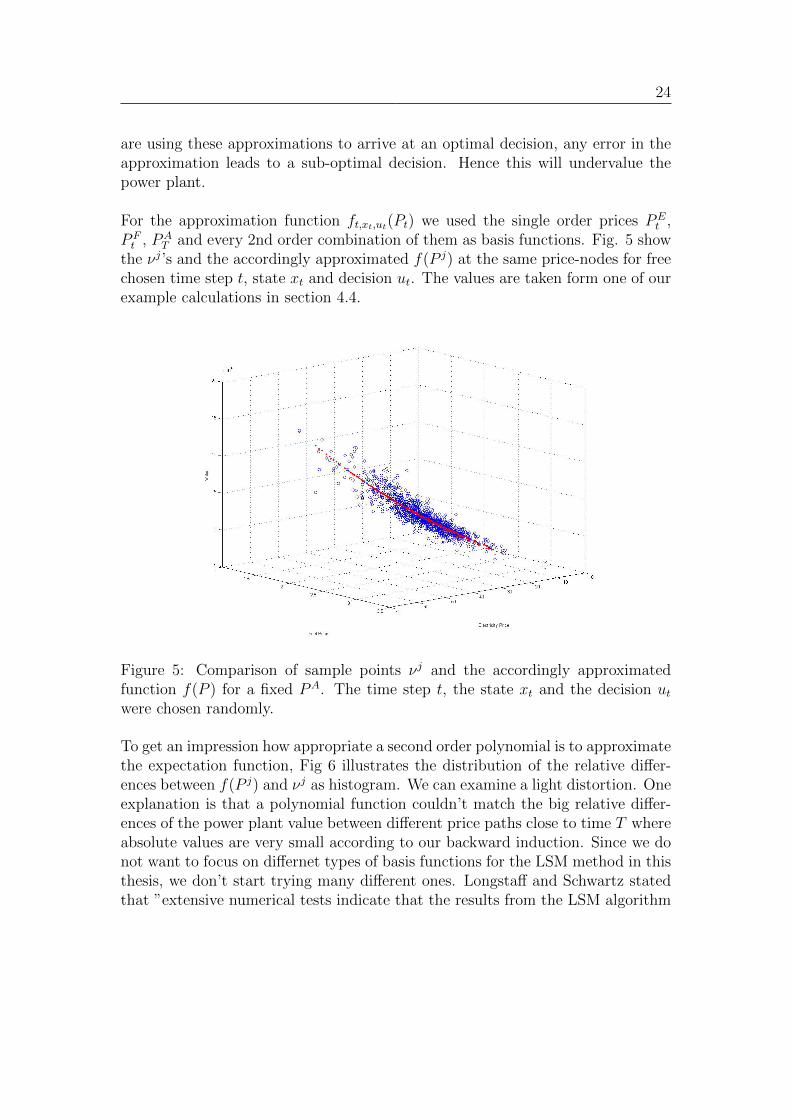
T and every 2nd order combination of them as basis functions. Fig. 5 showthe νj’s and the accordingly approximated f(P j) at the same price-nodes for freechosen time step t, state xt and decision ut. The values are taken form one of ourexample calculations in section 4.4.
Figure 5: Comparison of sample points νj and the accordingly approximatedfunction f(P ) for a fixed PA. The time step t, the state xt and the decision utwere chosen randomly.
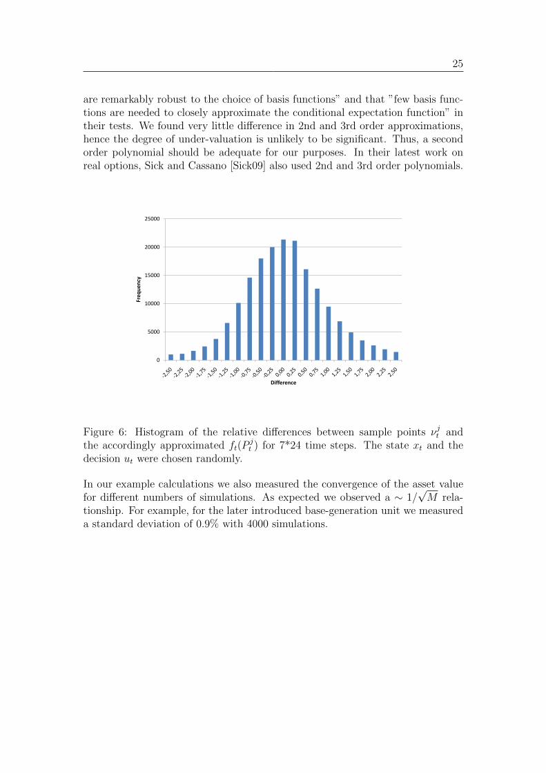
To get an impression how appropriate a second order polynomial is to approximatethe expectation function, Fig 6 illustrates the distribution of the relative differ-ences between f(P j) and νj as histogram. We can examine a light distortion. Oneexplanation is that a polynomial function couldn’t match the big relative differ-ences of the power plant value between different price paths close to time T whereabsolute values are very small according to our backward induction. Since we donot want to focus on differnet types of basis functions for the LSM method in thisthesis, we don’t start trying many different ones. Longstaff and Schwartz statedthat ”extensive numerical tests indicate that the results from the LSM algorithm
25
are remarkably robust to the choice of basis functions” and that ”few basis func-tions are needed to closely approximate the conditional expectation function” intheir tests. We found very little difference in 2nd and 3rd order approximations,hence the degree of under-valuation is unlikely to be significant. Thus, a secondorder polynomial should be adequate for our purposes. In their latest work onreal options, Sick and Cassano [Sick09] also used 2nd and 3rd order polynomials.
10000
15000
20000
25000
Frequency
0
5000
10000
15000
20000
25000
Frequency
Difference
Figure 6: Histogram of the relative differences between sample points νjt andthe accordingly approximated ft(P
jt ) for 7*24 time steps. The state xt and the
decision ut were chosen randomly.
In our example calculations we also measured the convergence of the asset valuefor different numbers of simulations. As expected we observed a ∼ 1/
√M rela-
tionship. For example, for the later introduced base-generation unit we measureda standard deviation of 0.9% with 4000 simulations.
26
4 Implementation aspects
The following section provide key figures about the Monte Carlo simulation ofthe price paths, the calibration of price parameters to historical market data andthe efficient implementation of the model algorithm. Additionally, some results ofexample calculations are presented. Here the asset properties are chosen accordingto typical, real world power plants. Furthermore, two short analysis show thebehaviour of the asset value when input parameters or asset constraints change.
4.1 Monte Carlo simulation
To simulate random price paths for Monte Carlo valuation the transition equa-tion for each price process is needed. We begin with the transition equation forelectricity prices according to the mean reverting process (6):
Pt+∆t = Pte−κE∆t exp
[(1− e−κE∆t)Lt + σE
√(1− e−2κE∆t)
2κEΦEt
](43)
with ΦE a collection of i.i.d. standard normal random variables. Here ∆t is theinfinitesimal time step. The transition equation for fuel prices according to the2-factor Schwartz-Smith model (13) is
χt+1 = χte−κχ∆t − λχ 1−e−κχ∆t
κχ+ σχ
√1−e−2κχ∆t
2κχΦχt ,
ξt+1 = ξt + µ∆t+ σξ√
∆tΦξ,P Ft+1 = eχt+1+ξt+1s(t),
(44)
with Φχ,Φξ collections of i.i.d. standard normal random variable. Determiningthe value of s(t), we have to be careful about the right season at time t0 when theprocess starts. For proofs of (43) and (44) see [Dixit94], p.76. Last but not leastthe transition equation for allowance prices according to (15) is:
Pt+1 = Pt exp(µA∆t+ σA
√∆tΦA
t + ln(Jt)ΦNt
)(45)
where ΦN is a collection of i.i.d events of a standard Poisson process with λ meanarrivals per time. Above we defined k := E[J − 1] = exp(µJ + σJ2/2) − 1. If wetransform this equation to express µJ with k, we get the jump amplitude:
ln(Jt) = ln(k + 1)− σJ2
2+ σJΦJ
t . (46)
Here ΦA,ΦJ are collections of i.i.d. standard normal random variables. So for thePoisson process we simulate the jump times from an exponential distribution firstand then simulate ΦJ only for these times. To include the correlations given in
27
(18) into the simulation, we generate four independent collections of i.i.d. standardnormal random events and multiply them with the Cholesky decomposition matrixU of the correlation matrix
Before we can simulate price paths according to (43), (44), (45), (46) and (47),we have to find appropriate values for all relevant parameters. To obtain these,we calibrate each price process to current or historical market data of liquidlytraded contracts. The following sections describe how we did this for our examplecalculations.
4.2.1 Electricity prices
First, we observed end-of-day prices of hourly contracts from the intraday spotmarket of the European Energy Exchange (EEX) over a two-year period from19.01.2007 to 19.01.200914. Then, for each of the 24 one-hour contracts, we tookthe 60 day average of historic log-prices15 as an estimation of LEt . By applying alinear regression on the same data as an alternative and comparing the results, wefound out that both estimates for LEt are very close. The results can be found inTable 4. Secondly, after bringing the contracts into the right chronological order,we used the following description of log-price movements, derived from (44):
xt+1 − xt = (1− eκ∆t)(Lt − xt) + εt= a+mxt + εt,
(48)
to regress κ by minimizing the mean square error to the market log-returns. Thestandard deviation from this linear regression multiplied by
√−2κ/(e−2κ − 1) is
an appropriate estimation of the volatility σE. Note that the time unit of theseestimations is one hour.
4.2.2 Fuel prices
The power plant model can be applied to oil, coal, gas and biomass as fuels. Sincean observation and comparison of all different fuel types would to go beyond the
14Source: Bloomberg15with a lower bound c > e 10.00
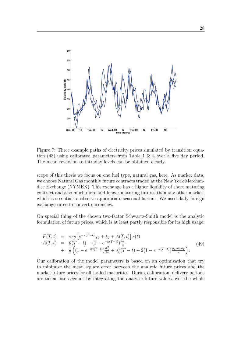
Figure 7: Three example paths of electricity prices simulated by transition equa-tion (43) using calibrated parameters from Table 1 & 4 over a five day period.The mean reversion to intraday levels can be obtained clearly.
scope of this thesis we focus on one fuel type, natural gas, here. As market data,we choose Natural Gas monthly future contracts traded at the New York Merchan-dise Exchange (NYMEX). This exchange has a higher liquidity of short maturingcontract and also much more and longer maturing futures than any other market,which is essential to observe appropriate seasonal factors. We used daily foreignexchange rates to convert currencies.
On special thing of the chosen two-factor Schwartz-Smith model is the analyticformulation of future prices, which is at least partly responsible for its high usage:
F (T, t) = exp[e−κ(T−t)χ0 + ξ0 + A(T, t)
]s(t)
A(T, t) = µ(T − t)− (1− e−κ(T−t))λχκ
+ 12
((1− e−2κ(T−t))
σ2χ
2κ+ σ2
ξ (T − t) + 2(1− e−κ(T−t))ρχξσχσξ
κ
).
(49)
Our calibration of the model parameters is based on an optimization that tryto minimize the mean square error between the analytic future prices and themarket future prices for all traded maturities. During calibration, delivery periodsare taken into account by integrating the analytic future values over the whole
29
delivery period. Due to time we can’t go into details here. Another recommendedestimation method would be a filtering technique like [Kalman60]. We had theopportunity to re-calibrate the implied parameters every day over a six-monthperiod and observed very little variation in values, which is a good indicator thattwo-factor Schwartz-Smith is an appropriate model.
Jan. 01 Jan 02 Jan 033
3.5
4
4.5
5
5.5
6
time (month)
Na
tura
l G
as (
€/m
mB
TU
)
Figure 8: Three example paths of Natural Gas prices simulated by transitionequation (44) using calibrated parameters from Table 1 & 2 over a two yearperiod. The seasonal shape can be observed.
4.2.3 Emission allowance prices
According to European regulatory requirements for carbon emissions, which arebriefly described in the Appendix, a CO2 allowance can be delivered for a specifiedamount of emission that was produced at an arbitrary time point of the year. Ifwe think in terms of commodities, the ’delivery period’ of a carbon future, whichholds this allowance to emit CO2, is the whole year. Thus, the front-year carbonfuture price can be interpreted as a kind of spot price for CO2 emissions.
Furthermore, as we see in Figure 4, carbon futures on different maturities havevery similar price movements. In fact, one can measure a correlation of 99% be-tween two certificates in sequence. Hence, for the parameter calibration of the
30
assumed spot process (15), we only considered the front-year future history. Wetook observed market prices over a two year period from 19.01.2007 to 19.01.2009and apply a Maximum Likelihood Estimation (MLE). The estimator is the (log-)probability density function of the Merton jump-diffusion model (15), which canbe found in closed form using Fourier Transformation techniques on the Charac-teristic function (proof see e.g. [Labahn G.]).
pdf(x) =e−λT√
2π
∞∑n=0
(λT )n
n!
e− (µAT+nµJ−x)2
2(Tσ2A
+nσ2J
)√Tσ2
A + nσ2J
(50)
4.2.4 Correlations
Firstly, we measured the 24-hour average of electricity price for each observed dayand calculated daily returns. Additionally, we took the daily returns of the front-year future for emission allowances, the daily returns of the generic front-monthNatural Gas future for χ and the daily returns of the last generic Natural Gas fu-ture for ξ. With these four histories of daily returns, each over a two-year period,all correlations between PE, χ, ξ and PA can be estimated. The results can befound in Table 3. All correlations found out to be tiny except for ρχξ. Especiallythe zero correlation between electricity and Natural Gas and the negative corre-lation between electricity and emission allowances are conspicuous. An argumentfor the former could be that electricity traders are focusing on actual, local powerdemand - standard market instruments are regional one-day ahead auctions - andNatural Gas traders are looking for longer periods - standard market instrumentsare monthly Future contracts with a one-month delivery period. An argumentfor the later could be that higher power prices make regenerative power assetsmore valuable and emission would decrease in the long run. But these are justhypotheses.
Table 4: Hourly LEt values, estimated from one-hour period contracts traded atthe intraday spot market at the EEX from Dec 2008 till Jan 2009.
32
4.3 The algorithm
Before we present some results from example valuations of power assets with typ-ical constraints, we want to give a short overview of the numerical algorithm.Once more, a real option valuation is more complex than other path-dependentinstruments. Beside the high path-dependency, a valuation algorithm must con-sider several states simultaneously. Furthermore, at every valuation point on thesimulated paths, at every node on the extended trees (if using forests) or on everygrid point (if using a three-dimensional mesh), the possibility of switching to otherstates must be considered and valued.
As described in section 3.2.1, for every state and every Monte Carlo path we muststep backwards in time from the asset’s maturity T to the actual valuation datet0 and find the optimal state to switch to at every time point. The decision ismade by estimating the expected value (35) for every possible decision via leastsquare regression, which is described in section 3.2.2.
A first possible optimization of the algorithm is to recognize, that in our powerplant model there are tcold + ton states in total but only for 2 + tcold − toff states,x ≤ toff or x = ton, can the operational decisions affect the future state. In allother states, toff < x < ton, the operational decision can optimize the clean sparkspread but the future state is deterministic. This should be considered when al-locating cash.
A second simplification is the pre-generation of the complete, optimal clean sparkspread paths. In section 2.3 we defined the variable operational and maintenancecosts V OMt(xt, ut) for a fixed price path on every time point t, for every statext and for every decision ut. The special trick was to include all predictable in-stant and future losses like losses from changing operational level to optimumor start up fuel costs. With this technique V OMt(xt, ut) looks a little bit morecomplex than defining only actual losses when they appear but gives us the oppor-tunity to simulate the discrete Monte Carlo price paths and calculate Πc,j(q∗t ) andV OM j
t (xt, ut) in advance. The following pseudo-code shows the full algorithm tovaluate the real option:
1. simulate M Monte Carlo price path Pjj∈M according to (43), (44), (45),(46) and (47) using parameters from Table 4, 1, 2 & 3
2. calculate Πc,j(q∗t ) ∀j ∈ [1,M ], t ∈ [t0, T ] according to (3) and (22)
3. calculate V OM jt (xt, ut), ∀j ∈ [1,M ], t ∈ [t0, T ], xt ∈ X and ut ∈ 0, 1
according to (29)
33
4. calculate V jT (xT ), ∀j ∈ [1,M ], xT ∈ X according to (32)
5. for t = T − 1 until t0 do (t = t− 1):
(a) for all xt ∈ X do:
i. calculate switching cash flow sc(xt, 0, Pjt ) and sc(xt, 1, P
jt ) accord-
ing to (34) and νj(xt, 0, Pjt ) and νj(xt, 1, P
jt ) according to (38)
∀j ∈ [1,M ]
ii. calculate the coefficients bkt through regression according to (61)
iii. make decision ujt(xt) according to (40) ∀j ∈ [1,M ]
iv. calculate V jt (xt) according to (41) ∀j ∈ [1,M ]
6. calculate V0(x0) = 1/M∑
j Vj
0 (x0).
4.4 Example valuations
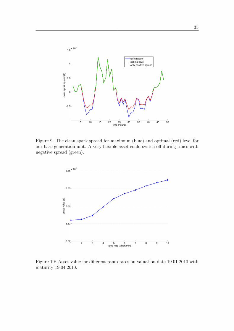
In this section we analyse how changes in some of the path-dependent constraintsaffect the value of a generation asset. We do this by comparing assets with variousconstraints to a base-generation unit with typical constraints. The properties ofour base-generation unit, introduced in equations (19), (20), (26) & (29) can befound in Table 5. If not stated otherwise, for all calculations we used the calibratedmarket parameters from section 4.2.In our first example we will examine different ramp rates rh. The ramp ratemainly defines the time needed for the adjustment to the optimal operationallevel. Figure 9 should give an impression how the optimized level q∗ changes thevalue of the clean spark spread Πc without shutting down the power plant. Nowwe changed rh and revalued the asset leaving all other market parameters andconstraints untouched. Of course, we also kept the same random numbers for allcalculations. Figure 10 shows the results: a higher rh has only little affect on theaverage asset value - about 10.000 e per month.
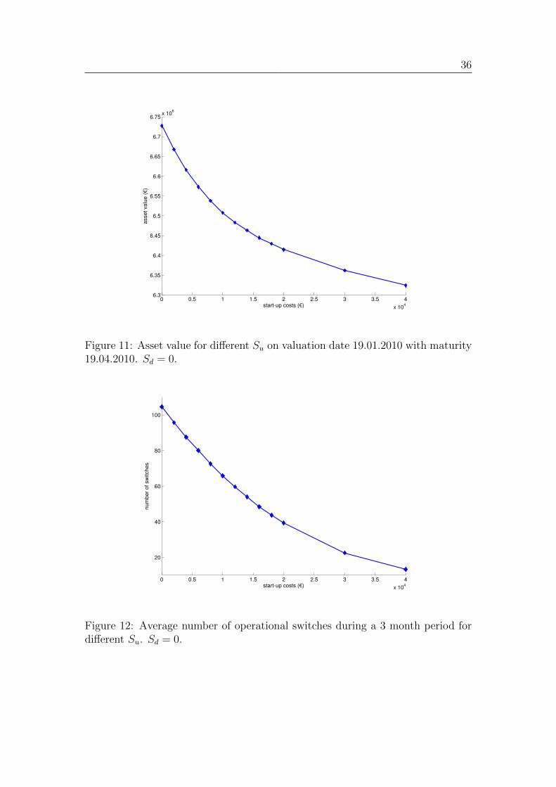
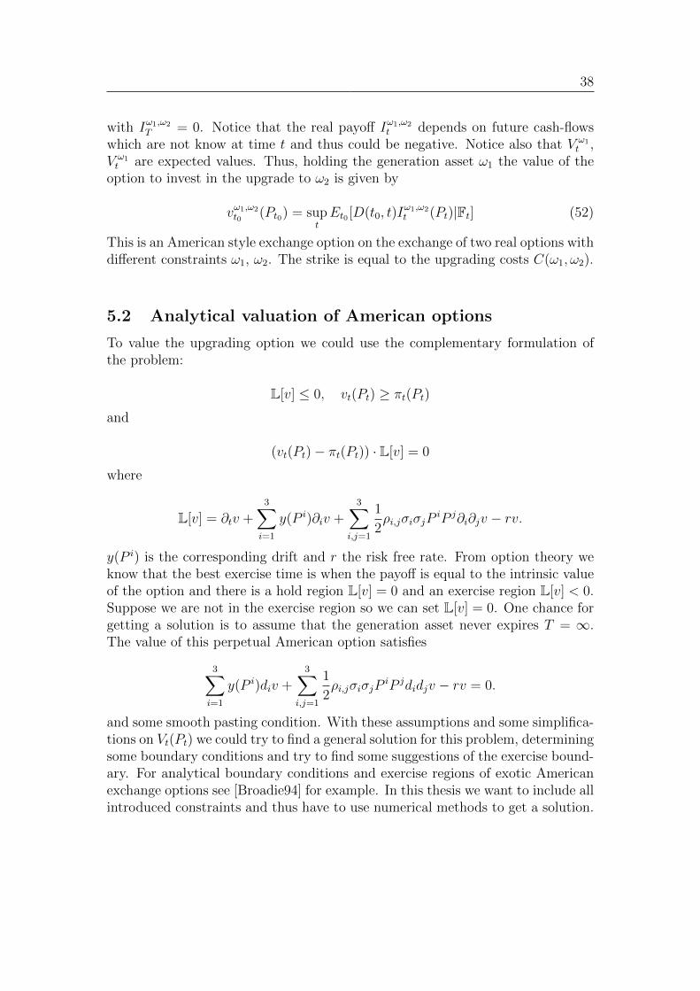
As a second example we regarding start-up Su and shut-down costs Sd. As wesaw in Figure 9 an immediate shut-down and start-up would be preferable atbeginning and end of negative clean spark spread periods. These times appearoften but persists only for a short while. Beside off- and on-times, shut-down andstart-up costs are the essential criteria for the decision to shut down or not. Inour analysis we changed Su to various levels and revalued the power plant. Wecould set Su = 0 without noticeable influence on the decision finding. Figure 11and Figure 12 illustrate the results.
Table 5: Typical constraints for a Combined Cycle Gas Turbine (CCGT). The in-formation come for the engineer at Didcot, the references given in the introductionand some google search on power plants.
In the literature generation assets are often grouped into three categories, Baseload, Mid-merit and Peaking units. Base-load units, as the name implies, handlethe base load of the grid. They have high start costs and have long minimum upand down times. Mid-merit units, on the other hand, tend to be less efficient thanbase-load units but typically have lower start costs, shorter minimum up/downtimes, and less time to ramp up to maximum capacity. Peaking units tend tohave high heat rates and are designed to be able to meet sudden peaks in demandand consequently have low start costs, short minimum up/down times, and canquickly ramp up to maximum generation, see [Clewlow09b]. Regarding these as-pects Clewlow and Strickland state that Base load, Mid-merit and Peaking unitscan be regarded as in-the-money, at-the-money and out-of-money options havingmore intrinsic or more extrinsic value. Here we don’t want to strictly divide phys-ical assets into categories but want to emphasise that crossings are smooth.
Now we could analyse a lot more sensitivities of constraints or market parametersand valuate different real units, but here we want to make a further step first. Wewant to value the possibility to changed a constraint, maybe through technologicalimprovements, as an exchange-option on two real options.
35
5 10 15 20 25 30 35 40 45 50
-0.5
0
0.5
1
1.5x 10
4
time (hours)
cle
an
sp
rak s
pre
ad
(€
)
full capacity
optimal level
only positive spread
Figure 9: The clean spark spread for maximum (blue) and optimal (red) level forour base-generation unit. A very flexible asset could switch off during times withnegative spread (green).
1 2 3 4 5 6 7 8 9 106.62
6.63
6.64
6.65
6.66x 10
6
ramp rate (MWh/min)
asse
t va
lue
(€
)
Figure 10: Asset value for different ramp rates on valuation date 19.01.2010 withmaturity 19.04.2010.
36
0 0.5 1 1.5 2 2.5 3 3.5 4
x 104
6.3
6.35
6.4
6.45
6.5
6.55
6.6
6.65
6.7
6.75x 10
6
start-up costs (€)
asse
t va
lue
(€
)
Figure 11: Asset value for different Su on valuation date 19.01.2010 with maturity19.04.2010. Sd = 0.
0 0.5 1 1.5 2 2.5 3 3.5 4
x 104
20
40
60
80
100
start-up costs (€)
nu
mb
er
of sw
itch
es
Figure 12: Average number of operational switches during a 3 month period fordifferent Su. Sd = 0.
37
5 Investing in new technologies
As we already pointed out in the introduction, there are a lot of new technologiesto improve efficiency of the generator or reduce the emission output of the plant.On the one hand, the actual energy market condition does not force an immediateinstallation for most of these innovations. On the other hand, by holding a phys-ical generation asset, the investor not only holds the real option but additionallysome American style options to install these new technologies. We will call themupgrading options. Thus, when an investor of a new power plant has to decidethe specifications, he should only compare the expected values of all possible con-straints but also consider the value of upgrading options - if there are any. Anexample is the investment in a new coal power plant and the choice is whether ornot to install a Carbon Capture Unit to reduce emissions. The question is: whatis the value of an upgrading option and when is the time to invest?
Luis M. Abadie and Chamorro [Chamorro08] as well as Stein-Erik Fleten andErkka Nasakkala [Nasakkala05] analysed investment options in power plants. Ei-ther they used DCF methods or they left out operational constraints and used aone dimensional stochastic process for the whole clean spark spread only, in orderto get analytical solutions. As mentioned before, the generation asset and espe-cially an upgrading option do not only depend on the pure clean spark spread. Ifwe think of an emission reduction installation without any side effects, the mar-ket conditions for emission allowances would be the essential criteria and not thespark spread itself. Here we want to go this different way. We want to use theintroduced real options as underlyings of the upgrading option while keeping eachprice process PE, PF , PA as uncertainty.
5.1 An American style exchange option on real options
To model an upgrading option we first define the set of all feasible values for allconstraint parameters as Ω. One point ω ∈ Ω represents a specific power plant.We denote the value of this power plant by V ω
t (Pt). For the sake of simplicity,the actual state xt are left out in the following. Especially for longer runningmaturities T , the actual state xt is insignificant for the whole value Vt. Now, atechnical improvement would change the power plant ω1 to a plant with differentspecifications ω2. Let C(ω1, ω2) denote the constant or deterministic costs for thistechnical improvement from ω1 to ω2. Then, the payoff value of the option is
Iω1,ω2t (Pt) = V ω2
t (Pt)− V ω1t (Pt)− C(ω1, ω2) (51)
38
with Iω1,ω2
T = 0. Notice that the real payoff Iω1,ω2t depends on future cash-flows
which are not know at time t and thus could be negative. Notice also that V ω1t ,
V ω1t are expected values. Thus, holding the generation asset ω1 the value of the
option to invest in the upgrade to ω2 is given by
vω1,ω2t0 (Pt0) = sup
tEt0 [D(t0, t)I
ω1,ω2t (Pt)|Ft] (52)
This is an American style exchange option on the exchange of two real options withdifferent constraints ω1, ω2. The strike is equal to the upgrading costs C(ω1, ω2).
5.2 Analytical valuation of American options
To value the upgrading option we could use the complementary formulation ofthe problem:
L[v] ≤ 0, vt(Pt) ≥ πt(Pt)
and
(vt(Pt)− πt(Pt)) · L[v] = 0
where
L[v] = ∂tv +3∑i=1
y(P i)∂iv +3∑
i,j=1
1
2ρi,jσiσjP
iP j∂i∂jv − rv.
y(P i) is the corresponding drift and r the risk free rate. From option theory weknow that the best exercise time is when the payoff is equal to the intrinsic valueof the option and there is a hold region L[v] = 0 and an exercise region L[v] < 0.Suppose we are not in the exercise region so we can set L[v] = 0. One chance forgetting a solution is to assume that the generation asset never expires T = ∞.The value of this perpetual American option satisfies
3∑i=1
y(P i)div +3∑
i,j=1
1
2ρi,jσiσjP
iP jdidjv − rv = 0.
and some smooth pasting condition. With these assumptions and some simplifica-tions on Vt(Pt) we could try to find a general solution for this problem, determiningsome boundary conditions and try to find some suggestions of the exercise bound-ary. For analytical boundary conditions and exercise regions of exotic Americanexchange options see [Broadie94] for example. In this thesis we want to include allintroduced constraints and thus have to use numerical methods to get a solution.
39
5.3 Numeric valuation
To value the American style upgrading option numerically we are following thesame steps as for the valuing of our real option in section 3. Our problem is tosolve
vω1,ω2t0 = sup
tEt0 [D(t0, t)I
ω1,ω2t (Pt)|Ft0 ] (53)
where Pt := (PEt , P
Ft , P
At ) and the boundary conditions at time T are given by
vω1,ω2
T (PT ) = max(Iω1,ω2
T (PT ), 0). (54)
Again we perform a backward induction and using Bellman’s principle of optimal-ity to get:
vω1,ω2t = max
(Et[I
ω1,ω2t (Pt)|Ft], Et[D(t, t+ 1)vω1,ω2
t+1 |Ft].)
(55)
To simplify notation we define
νext (Pt) := Et[Iω1,ω2t (Pt)|Ft]) (56)
νholdt (Pt) := Et[D(t, t+ 1)vω1,ω2
t+1 |Ft]) (57)
as the expected values and (55) becomes
vω1,ω2t = max
(νext (Pt), ν
holdt (Pt)
). (58)
We also leave out the index ω1, ω2 if it is clear. In section 3.2.2 we already havesimulated M price paths P j
t and calculated M value paths V j,ωit for j = 1..M ,
t = 1..T and i = 1, 2 accordingly; see (41). We can use these already simulatedpaths to value the exchange option by applying the least square Monte Carlomethod once more. In the following we take the average of V j,ωi
t (xt) over xt toexclude the irrelevant state. We assume again that νholdt (Pt) can be approximatedby a second order polynomial:
where for every time t, et,0 is a scalar, et,1 a 3-dimensional vector and et,2 a 3x3-Matrix of coefficients. For every Monte Carlo simulation P j
t at time t, j = 1..M ,we define
νhold,jt := D(t, t+ 1)vjt+1. (60)
which is (57) for one simulation P jt . Notice that due to the backward induction
we already know vjt+1 - defined in (62) - here. From these simulated νhold,jt J=1..M
40
we can now regress the coefficients et,k by minimizing the least square approxi-mation error:
et,k = arg minet,k
M∑j=1
(νhold,jt − fholdt (P j
t ))2
. (61)
Then we do the same kind of regression for νext but here we have to split into νω1t
and νω2t to approximate the expected value of V ω1
t and V ω1t separately by fω1
t andfω2t accordingly. After all, for every simulation P j
t , we set:
vjt =
νω2,jt − νω1,j
t − C if fω2t (P j
t )− fω1t (P j
t )− C > fholdt (P jt )
νhold,jt othewise(62)
Repeating this we go the steps backward in time as long as we reach t0. Then,
vt0 =1
M
M∑j=1
vjt0 . (63)
We notice that we have the opportunity to let the approximation of the conditionalexpectation ft not depend on all uncertainties but only on the essential ones. Asmentioned before, if we imagine of an CO2 filter without any additional costs orside effects Pt := (PE
t ) would be the right choice.
5.4 Examples
As an example we analyse the installation of a long-lived Carbon Capture andStorage (CCS) unit. On the one hand, a CCS is a huge plant by its own and cansave up to 90% CO2 output of a generation asset. On the other hand, it consumesa significant amount of the plant’s electricity output - about 15%. Additionally,there are CO2 transportation and storage costs - about 7.3e /t - and usual oper-ation and maintenance costs - about 550e /h. Since it haven’t been build before,the initial installation costs of a CCS unit could only be estimated to about 200Mio.e 16.
Yet, we haven’t introduced CO2 transportation and storage costs as well as self-used energy in our model. To do this we define fE as the proportional factor forCO2 output and fP as the proportional factor for electricity output. With thesefactors the clean spark spread in (3) changes to
16The values were taken from [Chamorro08] were more information on CCS units can befound.
41
Πc(q) = qfPPE −HR(q)P F − fEER(q)PA − (1− fE)ER(q)P S (64)
where P S is the constant price for CO2 transportation and storage. Furthermore,the optimal operational level defined in (22) becomes
q∗t = min(qmax,max(qmin,
(fPP
Et − fEE · PA
t − (1− fE)EP S
P Ft
− a1
)1
2a2
)).
(65)We do not change the start-up fuel and emission costs St in (24) because a CCSunit can’t operate during the start-up period. With these adjustments we cannow define the two generation assets ω1 and ω2 for our exchange option. Theirproperties are the same as for the base-generation asset in Table 5. The additionaland adjusted properties for ω1 and ω2 can be found in Table 6:
ω1 ω2
fP 100% fP 85%fE 100% fE 10%P S 0.0 e /t P S 7.3 e /tOM 600 e /h OM 1050 e /h
Cω1,ω2 200 Mio. e
Table 6: The different properties of the held asset without CCS ω1 and the up-graded asset with CCS ω2.
Since the biggest effect of a CCS installation is the emission reduction, the optionvalue vω1,ω2 strongly depends on the emission allowance price level PA
t . If T isfixed, the question of best exercise becomes: at which price level PA
0 the intrinsicoption value is equal to the payoff? Thus, we analysed the behaviour of the up-grade option vω1,ω2
0 and the payoff Iω1,ω2
0 under different PA0 . In the first run we
didn’t change PE and P F . Figure 13 shows the results17.
We observed that the value of the CCS is virtually zero for quite a large range ofallowance prices. For higher PA
0 the option value and the payoff seems to converge,but they do not - see Figure 14. The reason here is, that the electricity price levelleft unchanged and does not allow for the higher emission allowance costs. Thus,the clean spark spread Πt decrease under the OM level, even for ω2. At thatpoint, the electricity generation becomes unprofitable and V ω2 , vω1,ω2 decrease.
17Due to runtime, we reduced T and changed C accordingly
42
15 20 25 30 35 40
-2
-1
0
1
x 106
emission allowance price (€)
va
lue
(€
)
Figure 13: The value of the CCS upgrade option (green) and its payoff (blue)according to Table 6 with runtime T = 3 month and suitable investment costsC = 1.250.000 e .
20 30 40 50 60 70 80 90 100
-5
0
5
x 105
emission allowance price (€)
va
lue
(€
)
Figure 14: The value of the CCS upgrade option (green) and its payoff (blue) forhigh PA
0 according to Table 6 with runtime T = 1 month and suitable investmentcosts C = 416.666 e .
43
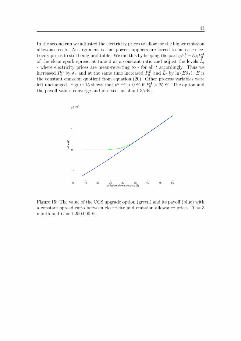
In the second run we adjusted the electricity prices to allow for the higher emissionallowance costs. An argument is that power suppliers are forced to increase elec-tricity prices to still being profitable. We did this by keeping the part qPE
0 −ERPA0
of the clean spark spread at time 0 at a constant ratio and adjust the levels Lt- where electricity prices are mean-reverting to - for all t accordingly. Thus weincreased PA
0 by δA and at the same time increased PE0 and Lt by ln (EδA). E is
the constant emission quotient from equation (20). Other process variables wereleft unchanged. Figure 15 shows that vω1,ω2 > 0 e if PA
0 > 25 e . The option andthe payoff values converge and intersect at about 35 e .
10 15 20 25 30 35 40 45 50
-1
0
1
2x 10
6
emission allowance price (€)
va
lue
(€
)
Figure 15: The value of the CCS upgrade option (green) and its payoff (blue) witha constant spread ratio between electricity and emission allowance prices. T = 3month and C = 1.250.000 e .
44
6 Conclusions
In this thesis we introduced a model for valuing generation assets which consideran own stochastic process for each price uncertainty of the clean spark spread. Weincluded many different but typical power plant properties into the model at thesame time. The resulting real option problem was solved by backward inductionusing a least square Monte Carlo method. With this model one can estimate thevalue for different types of generation assets. Especially when a power supplier hasto extend or rebuild his portfolio of power plants he could estimate the expectedprofits. Additionally, he could analyse the affect of the asset profits and operationmoods when there are essential changes in the energy market and he could figureout if an asset with different properties would show a different behaviour.
Beside the asset value, operational states and switching decisions are importantissues for a power plant operator. Our real option model support a concrete deci-sion for the actual state and a decision path according to price movements whichcan be used for a running unit. Especially the operator can figure out if it isvaluable for a specified unit to switch off during the low-price period at night ornot. Surely, after some time the model parameters must be recalibrated to thechanged market.
Generation asset runtimes may be up to 40 years. This is a known problem forstochastic valuation of generation asset because the maturities of market contractscomes up to at least 10 years. Furthermore long maturing contracts becomes veryilliquid. Thus, it is highly questionable if the calibrated parameters of the stochas-tic price processes could describe the behaviour of prices for longer maturities. Inour example calculation we only used shorter maturities to avoid this kind ofproblem.
In section 5 we consider that a generation asset always comes with options toupgrade the plant properties and its constraints. We showed a way to value thesekinds of options on real options. Here we could make full use of our model withthree individual described price processes. A model with a single process for theclean spark spread could not capture the origin of the differences. In our CCSexample we could find boundaries for emission allowance prices where it is optimalto exercise. An emission allowance prices above this point would bring no use foremission abatement - in our model world - but increase power prices.
There are a lot of open issues and some possible extension of our model whichleaves space for further analyses. At the end, we want to list a few here:
45
• A more complex but adequate model for electricity prices would be a regimeswitching process that consists of a spike regime and a base regime - see forexamples [Ronn02]. This model would take care of observable price spikesin the electricity market that are occurring through supply lacks due tounscheduled or forced outages.
• More power plant properties and operational constraints could be consideredwhich leads us to a wider range of operational states and possible decisions.A high sophisticated approach could even consider the opportunity to resellstored fuel of the fuel stack.
• To improve the least square Monte Carlo approach, one could compare dif-ferent sets of base-function and provide additional details on adequacy andconvergence. On the other side, the same regression function could be usedfor more than one time point to improve the algorithm speed. For example,one approximation function is regressed for every hour of the day but is usedfor several days of the month, to keep respect of the hourly electricity pricelevels.
• We could analyse hedging strategies with standard market future or optioncontracts.
• Last but not least we are sorry that there wasn’t time to look at specialaspects of coal, bio fuel or multi-fuel power plants.
46
The European Union Emission Trading Scheme
The EU-ETS is the largest multi-national, emissions trading scheme in the worldand is a major pillar of European Union climate policy18. The EU-ETS currentlycovers more than 10,000 installations which are collectively responsible for closeto half of the EU’s emission of CO2
19. Since 1 January 2005, companies that arepart of the EU-ETS have needed allowances to emit CO2. Sanctions are severeif companies decide not to comply with the regulation. If a firm does not delivera sufficient amount of allowances at the end of each year, it will have to pay apenalty and will have to deliver the missing EU allowances the following year.
There was a trial period (2005-2007) mainly intended for large industrial emit-ters. Each Member State set up its own National Allocation Plan (NAP) whichmust indicate how many emission allowances the Member State intends to issuealtogether. The Member must allocate at least 95% of allowances for this pe-riod free of charge20. This approach has been criticized as giving rise to windfallprofits, being less efficient than auctioning, and providing too little incentive forinnovative new competition to provide clean, renewable energy. To address theseproblems, the European Commission proposed various changes in a January 2008package - start of the first Kyoto commitment period (2008-2012) - including theabolishment of NAP’s from 2013 and auctioning a far greater share (60%) of emis-sion permits.
The EU scheme used to be a system of climate change policy that was com-pletely independent of International Climate Change Policy such as the UnitedNations’ Framework Convention on Climate Change (UNFCCC, 1992) or the Ky-oto Protocol that was subsequently (1997) established under it. When the KyotoProtocol came into force on 16 February 2005, the EU ETS had already becomeoperational. Only later, the EU decided to accept Kyoto flexible mechanism cer-tificates as compliance tools within the EU ETS. The Linking Directive allowsoperators to use a certain amount of Kyoto certificates from flexible mechanismprojects in order to cover their emissions21. According to the Kyoto Protocol, theEuropean Union must reduce its emissions by 8% below the 1990 levels during2008 to 201222.
18Oxford Journals, Review of Environmental Economics and Policy, 200719http://en.wikipedia.org/wiki/European Union Emission Trading Scheme20Federal Ministry for the Environment, Nature Conservation and Nuclear Safety, National
Allocation Plan for the Federal Republic of Germany, March 200421http://en.wikipedia.org/wiki/Clean Development Mechanism22United Nations, Kyoto Protocol to the United Nations Framework Convention On Climate
Change,1998
47
Like the Kyoto trading scheme, the EU scheme allows a regulated operator to usecarbon credits in the form of Emission Reduction Units (ERU) to comply withits obligations. A Kyoto Certified Emission Reduction unit (CER), producedby a carbon project that has been certified by the UNFCCC’s Clean Develop-ment Mechanism Executive Board, or Emission Reduction Unit (ERU) certifiedby the Joint Implementation project’s host country or by the Joint Implementa-tion Supervisory Committee, are accepted by the EU as equivalent. Thus one EUAllowance Unit of one tonne of CO2 (EUA) was designed to be identical with theequivalent Assigned Amount Unit (AAU) of CO2 defined under Kyoto. Hence,because of the EU’s decision to accept Kyoto-CERs as equivalent to EU-EUAs,it will be possible to trade EUAs and UNFCCC-validated CERs on a one-to-onebasis within the same system.
48
References
[Baron01] Baron M., Rosenberg M., Sidorenko N., Modelling and Predictionwith Automatic Spike Detection, Energy and Power Risk Manage-ment, pp. 36-9, October 2001
[Barz02] Barz G., Tseng C.-Li, Power Plant Operations and Real Options,Real Options and Energy Management by Ehud I. Ronn, page 255,Risk Waters Group Ltd, 2002
[Bellman57] Bellman R., Dynamic Programming, Princeton University Press,1957
[Broadie94] Broadie M., Detemple J., The Valuation of American Options onMultiple Assets, Scientific Series, Montreal, Septembre 1994
[Chamorro08] Abadie L.M., Chamorro J.M., European CO2 prices and carboncapture investments, Elsevier, Energy Economics 30 (2008) 2992-3015, April 2008
[Clewlow09] Clewlow L., Meador D., Sobey R., Strickland C., Valuing Genera-tion Assets, Masterclass series at energyrisk.com, June 2009
[Clewlow09b] Clewlow L., Meador D., Sobey R., Strickland C., Lujun Liu J.,Valuing Generation Assets Using Monte Carlo Simulation, Master-class series at energyrisk.com, September 2009
[Daskal05] Daskalakis G., Psychoyios D., Markellos R., Modeling CO2 emis-sion allowance prices and derivatives: evidence from the EEX,ERIM Report Series ERS-2005-052-F&A, 2005
[Deng98] Deng S. , Johnson B., Sogomonian A., Exotic Electricity Optionsand the Valuation of Electricitiy Generation and Transmission, pre-sented at the Chicago Risk Management Conference, Chicago 1998
[Dixit94] Dixit A.K., Pindyck R.S., Investment under Uncertainty, PrincetonUniversity Press, Princeton, N.J., 1994
[Duevel01] Dueuvelmeyer, D., Untersuchungen zu Chancen und Risiken vonAnti-Trend-Strategien am Beispiel des DAX-Futures, TechnischeUniversity Chemnitz, den 11. Januar 2001
49
[Geman05] Geman H., Commodities and commodity derivatives, John Wiley &Sons Ltd, England 2005
[Hsu98] Hsu M., Using Financial Options Theory to Value and Hedge Nat-ural Gas Power Assets, presented at the EPRI’s Pricing Energy ina Competitive Market Conference, Washington D.C. 1998
[Hull02] Hull J.C., Options, Futures, and other Derivatives, Prentice Hall,July 2002
[Kalman60] Kalman R.E., A New Approach to Linear Filtering and PredictionProblems, Transaction of the ASME, Journal of Basic Engineering,1960
[Labahn G.] Labahn G., Closed Form PDF for Merton’s Jump Diffusion Model,University of Waterloo, Canada, May 2003
[Longstaff01] Longstaff F.A., Schwartz E.S., Valuing American Options by Simu-lation: A Simple Least-Squares Approach, The Review of FinancialStudies, 14(1), page 113, 2001
[Ludwig09] Ludwig S.E., Two Different Ways of Modelling Seasonality, Uni-versity of Oxford, March 2009
[Merton75] Merton R.C., Option Pricing When Underlying Stock Returns AreDiscontinuous, WP 787-75 Massachusetts Institute of Technology,April 1975
[Nasakkala05] Nasakkala E., Fleten S.-E., Flexibility and technology choice ingas fired power plant investments, Elsevier, Review of FinancialEconomics 14 (2005) 371-393, May 2005
[Ronn02] Ronn E. I., Real Options and Energy Management, Risk WatersGroup Ltd, 2002
[Trueck08] Truck S., Benz E., Modeling the price dynamics of CO2 emissionallowances, Elsevier B.V. 2008
[Tseng09] Tseng C.-Li, Zhu W., Dmitriev A., Variable capacity utilization,ambient temperature shocks and generation, asset valuation, Else-vier, Energy Economics 2009
[Schwartz97] Schwartz E.S., The Stochastic Behavior of Commodity Prices: Im-plications for Valuation and Hedging, The Journal of Finance, Vol.52, No.3, July 1997
50
[Schwartz00] Schwartz E.S, Smith J.E., Short-Term Variations and Long-TermDynamics in Commodity Prices, Management Science, Vol. 46, No.7, pp. 893-911, Jul. 2000
[Seppi02] Seppi D.J., Risk-Neutral Stochastic Processes for CommodityDerivative Pricing: An Introduction and Survey, Real Options andEnergy Management by Ehud I. Ronn, page 255, Risk WatersGroup Ltd 2002
[Sick09] Sick G., Cassano M. Valuation of a Spark Spread: an LM6000Power Plant, University of Calgary, May 2009
[Uhlenbeck30] Uhlenbeck G.E., Ornstein L. S., On the theory of Brownian Motion,Physical Review. 36, page 823–841, 1930
[Wood84] Wood A.J., Wollenberg B.F., Power Generation, Operation andControl, John Wiley & Sons, New York 1984