DISCUSSION PAPER SERIES Forschungsinstitut zur Zukunft der Arbeit Institute for the Study of Labor Valuing School Quality via a School Choice Reform IZA DP No. 4719 January 2010 Stephen Machin Kjell G. Salvanes
Transcript
DI
SC
US
SI
ON
P
AP
ER
S
ER
IE
S
Forschungsinstitut zur Zukunft der ArbeitInstitute for the Study of Labor
Any opinions expressed here are those of the author(s) and not those of IZA. Research published in this series may include views on policy, but the institute itself takes no institutional policy positions. The Institute for the Study of Labor (IZA) in Bonn is a local and virtual international research center and a place of communication between science, politics and business. IZA is an independent nonprofit organization supported by Deutsche Post Foundation. The center is associated with the University of Bonn and offers a stimulating research environment through its international network, workshops and conferences, data service, project support, research visits and doctoral program. IZA engages in (i) original and internationally competitive research in all fields of labor economics, (ii) development of policy concepts, and (iii) dissemination of research results and concepts to the interested public. IZA Discussion Papers often represent preliminary work and are circulated to encourage discussion. Citation of such a paper should account for its provisional character. A revised version may be available directly from the author.
IZA Discussion Paper No. 4719 January 2010
ABSTRACT
Valuing School Quality via a School Choice Reform* Among policymakers, educators and economists there remains a strong, sometimes heated, debate on the extent to which good schools matter. This is seen, for instance, in the strong trend towards establishing accountability systems in education in many countries across the world. In this paper, in line with some recent studies, we value school quality using house prices. We, however, adopt a rather different approach to other work, using a policy experiment regarding pupils’ choice to attend high schools to identify the relationship between house prices and school performance. We exploit a change in school choice policy that took place in Oslo county in 1997, where the school authorities opened up the possibility for every pupil to apply to any of the high schools in the county without having to live in the school’s catchment area (the rule that applied before 1997). Our estimates show evidence that parents substantially value better performing schools since the sensitivity of housing valuations to school performance falls significantly by over 50% following the school choice reform. JEL Classification: I2 Keywords: house prices, school performance, school reform Corresponding author: Kjell G. Salvanes Department of Economics Norwegian School of Economics and Business Administration Helleveien 30 N-5035 Bergen-Sandviken Norway E-mail: [email protected]
* We would like to thank Sandy Black, Steve Gibbons, Caroline Hoxby, Sandra McNally, Olmo Silva and numerous seminar and conference participants for some very helpful comments. We also thank Roger Bivand for his great help in producing the Figures.
1
1. Introduction
The way in which housing markets are affected by differences in local school quality is
an important economic and social phenomenon and a highly topical and politically
charged issue. All over the world, parents are concerned that they get the best education
for their children. Empirical evidence shows that parents are willing to pay significant
amounts of money to buy houses located in the catchment areas of better performing
schools.1
Many papers in this literature show there to be sizable and significant
capitalizations linked to school quality. However, an ongoing issue in this literature
concerns the means by which the impact of school quality on housing valuations is
identified. This is pertinent since the main empirical challenge is to ensure that results
capture only the portion of housing expenditures affected by variations in school quality,
and not due to other (observed and unobserved) housing characteristics or local
amenities.
Early work in this area tried to net out these correlated effects by conditioning on
a range of observables. More recent work has tried to deal more effectively with the
unobserved aspects. One strand considers house price differences across school
catchment area boundaries to remove unobserved heterogeneity that could contaminate
any house price-school quality relation seen in the data.2 Other researchers have adopted
a quasi-experimental approach based on the redrawing of catchment area boundaries.3
1 See the literature reviews of Black and Machin (2010) or Gibbons and Machin (2008). 2 There are by now quite a few boundary discontinuity papers. See, inter alia, the early papers by Bogart and Cromwell (1997) and Black (1999) and the more recent work combining the boundary approach with other empirical methods by Gibbons and Machin (2003), Gibbons, Machin and Silva (2009) or Bayer, Ferreira and McMillan (2007). 3 In the context of a loss of neighbourhood schools and re-districting in Cleveland, Bogart and Cromwell (2000) adopt a quasi-experimental approach based upon the redrawing of catchment area boundaries. Ries
2
Despite these advances in methodology, there remain concerns and worries about
identification. For example, some critics argue that administrative boundaries are
endogenous to housing prices, possibly because of differential growth over time or
because they have differing institutional features (e.g. in the US where local property
taxes may differ on either side of the boundary). Similarly quasi-experimental variations
based on redrawing boundaries are also likely to be endogenous to school quality and/or
house prices (i.e. there are correlated reasons as to why the boundaries were redrawn).
In this paper we therefore adopt a different approach to causally identify the
relationship between house prices and school quality. We also use a quasi-experiment,
but one that is very different to those used to date. We implement a research design
based on a school admissions reform. The reform increased pupil choice to high schools
by allowing mobility across catchment area boundaries that was not permitted before. We
use this variation (sometimes coupled with a boundary discontinuity approach) to identify
the relationship between house prices and school performance.
To be more specific, we study the change in school choice that took place in Oslo
county in 1997, where the school authorities opened up the possibility for every pupil to
apply to any high school. Prior to this, rigid catchment areas were present and children
had to attend schools in the area in which they resided. Thus to identify school quality
capitalization we are able to exploit both a time-series variation (through the school
choice experiment) as well as cross-sectional variation using neighbourhood
discontinuities generated by the catchment area approach that has been more commonly
used in the recent literature.
and Somerville (2004) also treat a redrawing of school catchment zones in Vancouver in January 2001 as an experiment that they claim exogenously induces changes in school quality that in turn can affect housing valuations.
3
Our estimates show that parents substantially value better performing schools.
They also show that school choice matters. When proximity to high school is the criterion
for admission, parents are prepared to pay significant amounts of money to live in the
catchment area of schools they prefer. However, once the reform occurred and the
residence based zoning criterion for admission was removed, the house price-school
performance relation was significantly weakened. Indeed, in most of the specifications
that we report the house price premium linked to school quality falls by at least 50
percent once school choice was introduced.
The rest of the paper is structured as follows. In Section 2 we discuss the key
features of the school choice reform. Section 3 describes the data and offers an initial
descriptive analysis. Section 4 presents the results, while Section 5 concludes.
2. The School Choice Reform
School Admissions in Norway
At elementary school level in Norway (for pupils aged 6-13 in grades 1-7) all
pupils are allocated to schools based on fixed school catchment areas within
municipalities. With the exception of some religious schools and schools using
specialized pedagogic principles, parents are not able to choose the school to which their
children are sent (except by moving neighbourhood). There is a direct link between
elementary school attendance and attendance at middle or lower secondary schools (ages
13-16/grades 8-10), in that elementary schools feed directly into these lower secondary
schools. In many cases, primary and lower secondary schools are also integrated.
4
Admissions procedures are different for upper secondary schools (attended by
pupils aged 16-19 in grades VG1-VG3), where they are administered at county level. In
some counties parents can freely choose schools, but in others children are allocated to
school based on well-defined catchment areas, or high school zones.
The Oslo School Choice Reform
The system for allocating pupils at elementary school in Oslo - by far the largest
county of Norway with half a million inhabitants4 - consists of a system of catchment
areas for 98 schools. These 98 elementary schools then link directly into 47 middle
schools. Before the 1997/1998 school year, there was a direct link between a group of
elementary/middle schools and a group of secondary schools such that pupils graduating
after the last year of middle school could choose only within six well-defined high school
zones. There was no possibility of applying outside the zones.5 Altogether there are 17
high schools in Oslo qualifying for an academic track (see Figure 1), and thus within each
zone there was on average around three high schools and eight middle schools.6
A change in high school admissions policy took place in the 1997/98 school year
(see Oslo kommune, 2005; Wærnes and Lindvig, 2000; Nordli-Hansen, 2006). In
February 1997 the municipality of Oslo (which also acts with the authority of a county
for secondary schools) decided to offer free choice at high school level. All fifteen year
olds were eligible to apply to any secondary school within Oslo from the school year
starting in August 1997. There had been a lot of discussion of this issue both in the press
4 Out of the total Norwegian population of four and a half million. 5 This rule of zones at the high school level was only used for high schools giving credits for entering college. This comprises about 85 percent of the pupil population. All vocational high schools had open enrolment prior to the reform. There are also two general high schools that, at least to a certain degree, had open enrolment prior to the reform. We exclude these from the empirical analysis. 6 The share of private schools at this level and at this time in Oslo comprised about 1 percent of the students (Nordli-Hansen, 2005).
5
and in the political arena from the fall of 1996, ensuring that parents and students were
well informed when the reform was enacted in the school year of 1997/1998.
Whilst at the time of the reform there was no public information on school
performance, there were very clear perceptions in the Oslo population (as in other parts
of the country) that pupil performance differences existed across schools.7 In addition, it
was clear what was considered as best performing schools were not equally distributed
across the city.8 Therefore, it was argued (mostly by right-center politicians in Oslo) that
a free choice system would improve allocation of talent in Oslo, as well as improving
accountability. Left oriented politicians, on the other hand, argued that free choice would
lead to elite schools and deprive schools located in the poorest areas of the county.9
From the school year 1997/98 onwards all students were able to apply to go to
high school anywhere within Oslo. Students ranked six schools according to their
preferences and the central school authorities in Oslo matched students to school based
on their average grades in 10th grade (the last year of lower secondary school). More
specifically, if some schools were over-subscribed, based on average grades students
were allocated to their second ranked school (and so on) until a match was found. The
grades were based on study of ten subjects from both exam results and assessment during
the year. Students were able to obtain grades from 1 to 6 in every subject (below in our
empirical work we consider three of these subjects: Mathematics, Norwegian and
English). One total grade then would be between 0 and 60, with the average being around
35. Only the central school authority was involved in the matching and not the schools
7 That the perception of how schools were ranked is also supported by the sociological literature (Nordli-Hansen, 2005), and by articles in the main newspapers around the time for applying to high schools. 8 Public information about school performance across high schools in Norway – league tables - became available from 2001 (see Raaum, Hægeland, Kirkebøen and Salvanes, 2004 for a description). 9 In 2005 the system of free choice was again changed to a combination of free choice and zoning.
6
themselves, so this was a one-sided matching process. Since the grades could vary
between 1 and 60, there does not appear to have been an issue of uniquely matching
students to schools. Indeed, it is clear that people had a strong knowledge of which
schools where considered the best, and certain schools had many more applications than
they had capacity to offer.
3. Data and Initial Descriptive Analysis
Data
Data on school zones were provided to us by the school authorities in Oslo and the exact
geo-codes were provided by the geo-map section of the Oslo municipalities. This office
also provided geo-codes for elementary and secondary schools in Oslo. We have matched
these to house price data from 1995 to 2002, comprising two and a half years of data on
house prices before the reform and five and a half years after the reform.
The geography of high school zones and schools in Oslo are laid out in the map in
Figure 1. It shows the six different high school zones (Center, East, North West, South,
South East and West). The Figure also shows catchment area boundaries for elementary
and secondary schools. From the Figure it is evident that most high schools are located in
Central Oslo and in the Western and North-Western Zones.
We use annual data on grade point averages from each secondary school in
Mathematics, Norwegian and English. These have also been provided by the education
authorities in Oslo. As already noted, the marks are scaled from 1 to 6, with 6 being the
highest mark. We use the high school pupil average over pupils, and then average over
the pre- and post-reform years. This should give a more ‘permanent’ measure of high
7
school performance, and is confirmed by the rankings of schools being very similar over
the years we study. The reason we average across schools within zones is that there was
choice across schools within zones.
The house price data covers transactions on all (used) houses and apartments sold
in Norway10, although we restrict the data set to Oslo for our purpose. The data is
collected by Statistics Norway (Lillegard, 1994) and the sales statistics are compiled from
two sources: the Register of Landed Property, Addresses and Buildings (GAB); and a
follow up survey conducted by Statistics Norway to obtain additional information on the
houses. These variables are: the age of the house, the size of the house in square metres,
the number of rooms, number of bathrooms, and year of renovation. It also contains
information on 6 categories of house type, from apartments in large high rises to villas.
The month of the transaction is given in the data. The response rate for the survey is
between 80 and 90 percent. This means that we have access to information on 80-90
percent of the census of all sold apartments and houses in Oslo.
From 1995 onwards it is possible to match in the identity of the owner and to link
this to register data.11 This was done by Statistics Norway using the personal identifier of
the buyer. This gives us a number of advantages. First, we can place all houses into their
relevant school zones. Second, we can link owners to a very extensive set of demographic
information. Third, we have annual geo-code for all inhabitants in Oslo so that we can
identify the demographic composition of school zones by year.
10 The data set does not include apartments owned by housing cooperatives since these properties are not traded freely in the market. 11 These register data are collected from other administrative sources and maintained by Statistics Norway. A description of these data sets is given in Møen, Salvanes and Sørensen (2004).
8
Table A1 in the Appendix presents descriptive statistics for the pre- and post
reform time periods. We have also defined a boundary sample covering all properties
within 500 meters of the catchment area boundaries. We use this sample since it is now
an established procedure in the literature to implement research designs treating
catchment area boundaries as discontinuities to identify the impact of school quality on
house prices (see, inter alia, Black, 1999; Gibbons and Machin, 2003; Kane, Staiger and
Reigg, 2005; Fack and Grenet, 2007), an approach we consider in more detail below.
Descriptive Statistics
Figure 2 shows the spatial distribution of high school grades across the city areas
of Oslo. Darker (lighter) shading corresponds to higher (lower) grades. It is clear that
schools in zones in the West; North-West and Centre do better.12 This corresponds
closely to the perceived ranking of parents in Oslo, as reported in the sociological
literature (Nordli-Hansen, 2005).
In Figure 3 we do the same exercise for house prices (measured in real NOK per
square metres). The Figure splits the house price distribution in 6 parts and again shows
higher (lower) mean prices in city areas in darker (lighter) shading. It is evident that the
high house price areas are also the West and North-West zones plus the Center zone,
which are the areas where the highest performing schools are located.
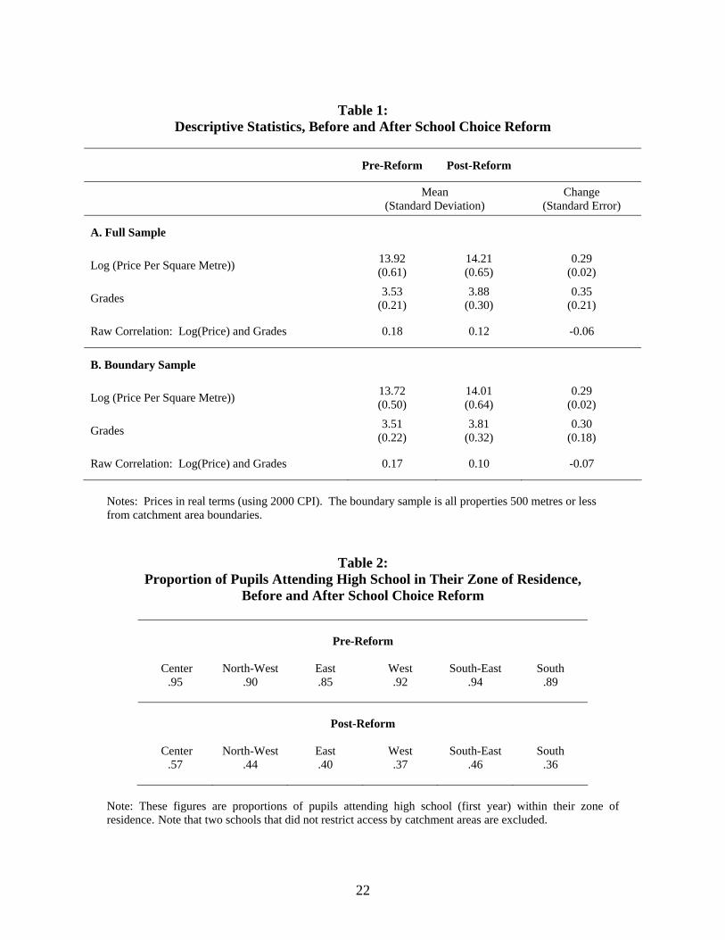
In Table 1 we present some descriptive statistics on house prices before and after
the school admissions reform and the simple correlation between log(house prices) and
school performance for various samples. The top Panel of the Table shows house prices
rose significantly between the two time periods, and that school grades went up a little
(but not by a statistically significant amount). It also shows a significant correlation 12 We have excluded the two schools in the Centre zone which had open access all the time.
9
between house prices and school performance in both the pre- and post-reform periods
but, interestingly, the correlation falls after the reform occurred. The lower Panel of the
Table considers the boundary sample defined as all properties within 500 meters of the
catchment area boundaries.13 It is interesting that very much the same pattern of change
of house prices and grades, and their correlations, is seen for this sub-sample.
One vital issue about the school reform is whether the opening up to school choice
did in fact alter high school attendance patterns. Table 2 shows the reform had a strong
impact on where students went to high school pre and post reform. In the pre-reform
period the vast majority of students (between 85-95 percent) attended a high school
within their zone of residence.14 After the reform, much more boundary crossing is seen
as only between 36 and 57 percent of the students went to a high school in the zone
where the student was living.
4. Methods and Results
Methods
At a particular point in time, say period t, a standard hedonic formulation15 relating log
(house prices) to school quality can be expressed as:
ististstist ut)s(e),g(s,γzβsp +++= (1) where pist is the log property price for house i in a neighbourhood or school catchment
zone s at time t, zist includes property, neighbourhood and demographic characteristics16,
13 We find similar results (in the descriptives and empirical work below) for cut-offs of 1000m and 250m. 14 There are likely to be several reasons why the pre-reform attendance rates are less than 100 percent, including some students moving in the middle of a school year, private schooling and school attendance outside Oslo county. 15 See Rosen (1974) for the classic exposition of the hedonic pricing approach and the review by Sheppard (1999).
10
sst measures school quality and the g(s, s(e), t) function contains various different fixed
effects, for school s, elementary school17 e (which is directly linked to school s as shown
in Figure 1 and as discussed in Section 2 above) and time t. Finally, uist is a random error
term.
This kind of function has been used in the existing literature to try to estimate β,
the sensitivity of house prices to (measured) school performance. One worry is that there
are unobserved variables which this approach cannot control for. Therefore, some studies
make use of the fact that there is a discontinuity at catchment area boundaries by
comparing houses on either side of school area boundaries, and thus effectively
controlling for unobserved characteristics of the houses or omitted neighbourhood
characteristics such as local public goods. This is a much more convincing approach, but
one worry that remains is that unobserved factors (like house maintenance) may grow
differently on either side of the borders. Moreover, even if houses were similar on either
side of the border when zone borders were originally established, houses may change
character over time as they are bought and sold. For example, it may be the case that if
one is willing to pay a premium to live in a school are with good school, it may also mean
that one is willing to invest more and maintain and improve the house.
The reform potentially changes the house price-school quality relation in a time
series context and we can use reform induced variations in school quality to get around
16 We present estimates that do and do not control for these characteristics as we remain uncertain about the plausibility of an exogeneity assumption about them owing to possible sorting by residents that is directly linked to the particular characteristics in question. 17 In Oslo there is a connection between elementary school attended and secondary school attendance, again working through fixed catchment zones although the link may not be too strong since even in the pre-reform period there was choice of high schools based on primary school marks within each zone. Hence, since there is a potential link between good primary schools/neighbourhoods and good high schools even after the reform. This is one reason why we also include elementary school fixed effects in some of our empirical specifications.
11
the problems linked to differential unobservables across boundaries. To do so we use
two, related but different, modelling strategies. First, we estimate equation (1) separately
for the pre-reform and post-reform time periods. Adding a k superscript (k = pre, post) to
(1) gives the equation
istk
istk
stkk
ist ut)s(e),(s,gzγsβp +++= (2) Thus we can study what happens to the school quality premium before and after
reform by testing the null hypothesis postpre ββ = .18 We implement this before-after
comparison for the full sample of housing transactions. We are also able to use the
discontinuity approach of controlling for additional common unobservables in the
boundary sub-sample. One feature of this is to generalise the g(.) function to include
boundary fixed effects, thus re-specifying as g(s, s(p), t, b), with b denoting a boundary:19
istk
istk
stkk
ist ub) t,s(e),(s,gzγsβp +++= (3) Our second approach recognises that the school choice reform induced policy
variation at the level of the admission zone, by permitting children to cross what were
previously non-crossable catchment area boundaries. The catchment area zones each
contained several high schools (around three on average). The idea behind this approach
is that the pre-reform capitalization is likely to be embedded in catchment area fixed
effects, αc. We therefore first estimate these catchment area fixed effects separately pre-
and post-reform, then relate them to school grades in a second stage at catchment area
level, c. 18 One way to think about this is that we are using a supply shock – the school reform – to identify the parameters in the hedonic price function for houses. 19 Use of boundaries amounts to assuming that unobserved factors affecting house prices change smoothly across space, and are not correlated with school quality differences across boundaries. Of course, there may be differences in sorting and unobserved house differences along borders. Our (effective) use of the school choice reform as an instrument, by estimating before and after reform, should enable us to avoid such potential problems.
12
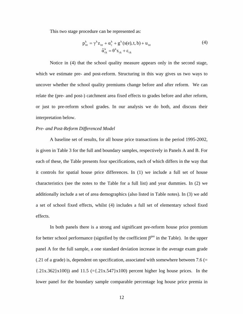
This two stage procedure can be represented as:
istkk
cistkk
ist ub) t,(s(e),gαzγp +++=
ckckkk
ck εsθα̂ +=
(4)
Notice in (4) that the school quality measure appears only in the second stage,
which we estimate pre- and post-reform. Structuring in this way gives us two ways to
uncover whether the school quality premiums change before and after reform. We can
relate the (pre- and post-) catchment area fixed effects to grades before and after reform,
or just to pre-reform school grades. In our analysis we do both, and discuss their
interpretation below.
Pre- and Post-Reform Differenced Model
A baseline set of results, for all house price transactions in the period 1995-2002,
is given in Table 3 for the full and boundary samples, respectively in Panels A and B. For
each of these, the Table presents four specifications, each of which differs in the way that
it controls for spatial house price differences. In (1) we include a full set of house
characteristics (see the notes to the Table for a full list) and year dummies. In (2) we
additionally include a set of area demographics (also listed in Table notes). In (3) we add
a set of school fixed effects, whilst (4) includes a full set of elementary school fixed
effects.
In both panels there is a strong and significant pre-reform house price premium
for better school performance (signified by the coefficient βpre in the Table). In the upper
panel A for the full sample, a one standard deviation increase in the average exam grade
(.21 of a grade) is, dependent on specification, associated with somewhere between 7.6 (=
{.21x.362}x100)) and 11.5 (={.21x.547}x100) percent higher log house prices. In the
lower panel for the boundary sample comparable percentage log house price premia in
13
the pre-reform period are between 7.0 and 10.4 percentage points. Thus in the pre-school
choice period with fixed catchment zones Oslo parents valued school quality very highly
indeed.
After the opening up to school choice, parents still strongly valued better school
performance, but the relationship with house prices significantly fell. This is shown by
the halving (or more) of the post-reform coefficient βpost shown in the Table. Indeed the
estimated coefficient falls very strongly and significantly (from -.18 to -.28 in the full
sample in Panel A and by a very similar -.18 to -.29 in the boundary sub-sample in Panel
B). All in all, this is very strongly suggestive of a significant impact of the opening up to
school choice on school quality related house price premia.20
One pertinent observation is that the house price premium does not fall to zero
when the catchment areas were removed. Presumably this is because transport costs still
remain, combined with the fact that persistent neighbourhood differences induced by the
former catchment areas remain. On the question of transport costs this generates a
willingness to pay to be closer to schools simply to reduce travel costs. Of course, school
locations do not change pre- and post-reform so our differencing across the pre- and post-
reform periods should not be affected by this.
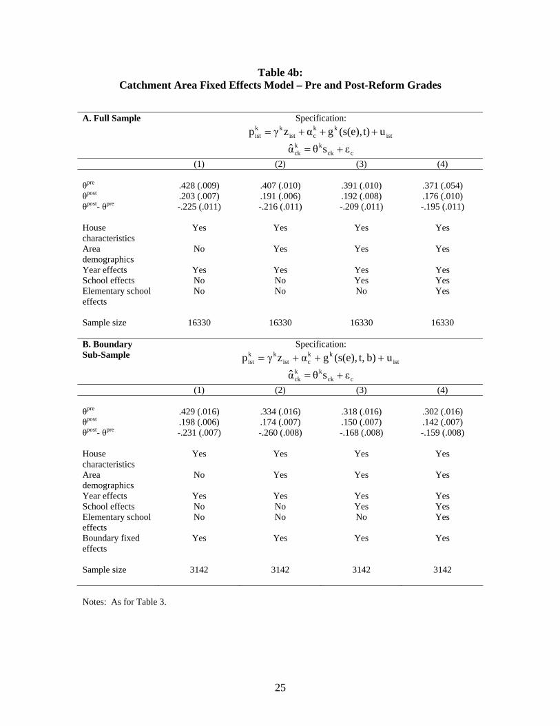
Catchment Area Fixed Effects Model
Tables 4a and 4b show results from the two stage approach. This, of course, is
similar to the fully differenced models in Table 3, but changes the focus to see how how
house price variations at the catchment area level vary with school quality change pre-
and post-reform. Tables 4a and 4b differ in which school quality measure is used. In
20 Inclusion of catchment area trends in all reported models made little difference and the key results remained intact.
14
Table 4a the catchment area fixed effects retrieved from the first stage are regressed on
pre-reform grades, whilst in Table 4b the same period grades are utilised. The story that
emerges is the same.21 Both Tables show a strong fall in the magnitude of the empirical
connection between house prices and school quality after the opening up to school
choice. In all specifications, this falls by 50 percent or more after the reform.
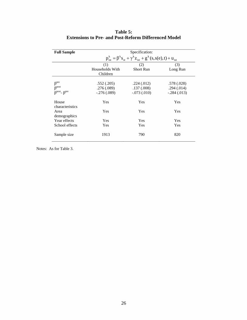
Extensions
In Table 5 we present some extensions and robustness checks. The very rich data
we have means that, unlike almost all studies in the literature, we know whether
households have children living in them. In (1) we thus consider results from the
differenced model for households with high school age children. For sample size reasons
we can do this only for the full sample, but the estimates are strikingly reassuring, with
the school quality premium falling by around 50 percent from .552 to .276.
In (2) and (3) we present (again for the full sample only) what we refer to as a
short run or 'instantaneous' sample (one year before reform, 1995-96, compared to one
year after, 1997-98) and a long run sample (one year before reform, 1995-96, compared
to five years later, 2001-02). Again reassuringly we find significant falls in the school
quality premium for both, but with there being stronger, more sizable effects in the long
run as compared to the short run 'instantaneous' impact.
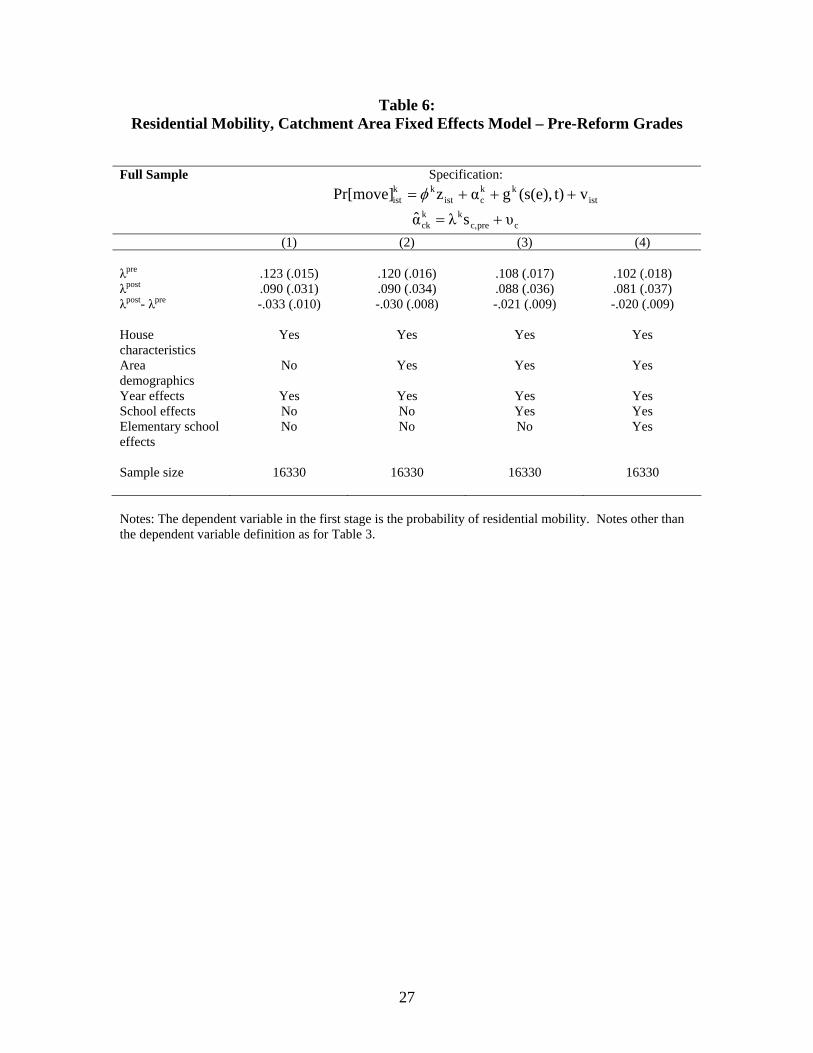
Residential Mobility Before and After the Reform
It is evident that another feature of the opening up to school choice would not
only be a reduced need for parents to pay for better school quality, but also a reduced
21 This is reassuring in that one may worry that estimates from the model including post-reform fixed effects could induce a bias as the first stage model does not capture pre-reform variation in school quality. This is not a problem in the models including pre-reform period fixed effects as school quality is assigned by the catchment area.
15
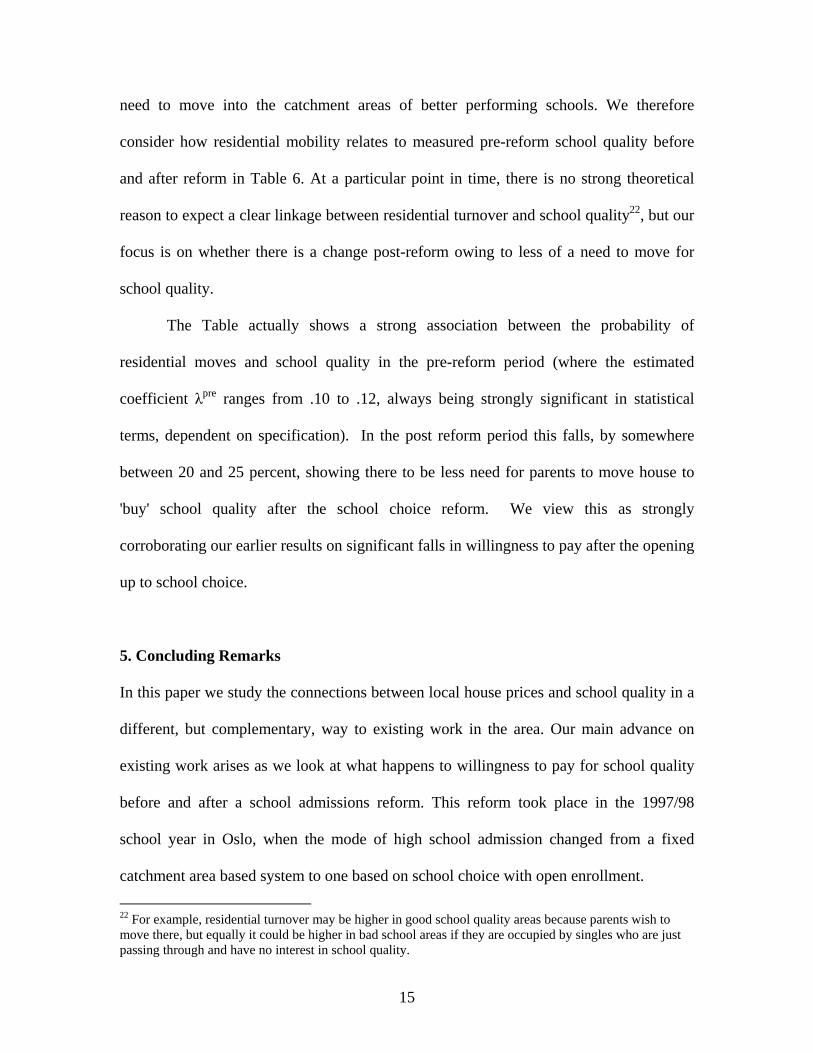
need to move into the catchment areas of better performing schools. We therefore
consider how residential mobility relates to measured pre-reform school quality before
and after reform in Table 6. At a particular point in time, there is no strong theoretical
reason to expect a clear linkage between residential turnover and school quality22, but our
focus is on whether there is a change post-reform owing to less of a need to move for
school quality.
The Table actually shows a strong association between the probability of
residential moves and school quality in the pre-reform period (where the estimated
coefficient λpre ranges from .10 to .12, always being strongly significant in statistical
terms, dependent on specification). In the post reform period this falls, by somewhere
between 20 and 25 percent, showing there to be less need for parents to move house to
'buy' school quality after the school choice reform. We view this as strongly
corroborating our earlier results on significant falls in willingness to pay after the opening
up to school choice.
5. Concluding Remarks
In this paper we study the connections between local house prices and school quality in a
different, but complementary, way to existing work in the area. Our main advance on
existing work arises as we look at what happens to willingness to pay for school quality
before and after a school admissions reform. This reform took place in the 1997/98
school year in Oslo, when the mode of high school admission changed from a fixed
catchment area based system to one based on school choice with open enrollment.
22 For example, residential turnover may be higher in good school quality areas because parents wish to move there, but equally it could be higher in bad school areas if they are occupied by singles who are just passing through and have no interest in school quality.
16
Our estimates based on the reform show evidence that parents substantially value
better performing schools. They also show that school choice matters. When proximity to
high school through residence in a fixed catchment area is the criterion for admission,
parents are prepared to pay significant amounts of money to live in the catchment area of
schools they prefer. The pre-reform magnitudes are in line with other work in the area
(perhaps towards the upper end), with a one standard deviation increase in test scores
implying a 7-10 percent higher level of house prices. However, once the reform occurred
and the proximity criterion for admission was removed, the house price-school
performance relation was significantly weakened, falling by a large magnitude with the
house price premium for school quality dropping by 50 percent or more compared to the
pre-reform time period.
17
References Bayer, P., F. Ferreira and R. McMillan (2007) A Unified Framework for Measuring
Preferences for Schools and Neighborhoods, Journal of Political Economy, 115, 588-638.
Black, S. (1999) Do Better Schools Matter? Parental Valuation of Elementary Education,
Quarterly Journal of Economics, 114, 578-599. Black, S. and S. Machin (2010) Housing Valuations of School Performance, forthcoming
in E. Hanushek, S. Machin and L. Woessmann (eds.) Handbook of the Economics of Education, Amsterdam: Elsevier.
Bogart, W. and B. Cromwell (1997) How Much More Is a Good School District Worth?,
National Tax Journal, 50, 215-232. Bogart, W. and B. Cromwell (2000) How Much is a Neighbourhood School Worth?,
Journal of Urban Economics, 47, 280-305. Fack, G. and J. Grenet (2007) Do Better Schools Raise Housing Prices? Evidence from
Paris School Zoning, Paris Ecole Normale Superieure, mimeo. Gibbons, S. and S. Machin (2003) Valuing English Primary Schools, Journal of Urban
Economics, 53, 197-219. Gibbons, S. and S. Machin (2008) Valuing School Quality, Better Transport and Lower
Crime, Oxford Review of Economic Policy, 24, 99-119. Gibbons, S., S. Machin and O. Silva (2009) Valuing School Quality Using Boundary
Discontinuities, Spatial Economics Research Centre, London School of Economics, Discussion Paper DP0018.
Kane, T., S. Riegg and D. Staiger (2005) School Quality, Neighborhood and Housing
Prices: The Impacts of School Desegregation, National Bureau of Economic Research Working Paper No. 11347.
Lillegard, S. (1994) Prisindekser basert på boligprisdatabasen. Møen, J., K. Salvanes and E. Sørensen (2004) Description of the Register Database at the
Norwegian School of Economics, mimeo, The Norwegian School of Economics. Nordli Hansen, M. (2005) Ulikhet i Oslo-skolen: Rekruttering og segregering, Tidsskrift
for Ungdomsforskning, 5, 3-26. Oslo kommune utdadanningsetatene (2005) Bakgrunnspapirer for Oslo Bystyrevedtak om
vedtak om inntaksregler for vidergående skole i Olso.
18
Hægeland, T., L. Kirkebøen, O. Raaum and K.G. Salvanes (2004) Marks Across Lower
Secondary Schools in Norway: What can be Explained by the Composition of Pupils and School Resources?, Rapport 11/2004, Statistics Norway.
Ries, J. and T. Somerville (2004) School Quality and Residential Property Values:
Evidence from Vancouver Rezoning, Working paper, Department of Economics, University of British Columbia.
Rosen, S. (1974) Hedonic Prices and Implicit Markets: Product Differentiation in Pure
Competition, The Journal of Political Economy, 82, 34-55 Sheppard, S. (1999) Hedonic Analysis of Housing Markets, in Handbook of Urban and
Regional Economics, (P. Cheshire, Ed.), Elsevier Science. Wærnes, J. and Y. Lindvig (2000) Fritt skolevalg eller sosial reproduksjon, Læringslaben.
19
Figure 1: High School Locations and Zones and Elementary and Secondary Catchment
Boundaries in Oslo, Pre-Reform
20
Figure 2: School Grades Pre-Reform
21
Figure 3:
House Prices Pre-Reform
22
Table 1:
Descriptive Statistics, Before and After School Choice Reform
Pre-Reform Post-Reform
Mean (Standard Deviation)
Change (Standard Error)
A. Full Sample
Log (Price Per Square Metre)) 13.92 (0.61)
14.21 (0.65)
0.29 (0.02)
Grades 3.53 (0.21)
3.88 (0.30)
0.35 (0.21)
Raw Correlation: Log(Price) and Grades 0.18 0.12 -0.06
B. Boundary Sample
Log (Price Per Square Metre)) 13.72 (0.50)
14.01 (0.64)
0.29 (0.02)
Grades 3.51 (0.22)
3.81 (0.32)
0.30 (0.18)
Raw Correlation: Log(Price) and Grades 0.17 0.10 -0.07
Notes: Prices in real terms (using 2000 CPI). The boundary sample is all properties 500 metres or less from catchment area boundaries.
Table 2: Proportion of Pupils Attending High School in Their Zone of Residence,
Before and After School Choice Reform
Pre-Reform
Center North-West East West South-East South
.95 .90 .85 .92 .94 .89
Post-Reform
Center North-West East West South-East South .57 .44 .40 .37 .46 .36
Note: These figures are proportions of pupils attending high school (first year) within their zone of residence. Note that two schools that did not restrict access by catchment areas are excluded.
Year effects Yes Yes Yes Yes School effects No No Yes Yes Elementary school effects
No No No Yes
Boundary fixed effects
Yes Yes Yes Yes
Sample size 3142 3142 3142 3142
Notes: The dependent variable is ln(sales price). School grades are an average of Norwegian and Math and English. Robust standard errors allowing for clustering at the high school catchment area level in parentheses. Sample is limited to all sales 1995-2002. House characteristics are: number of rooms, number of bathrooms, wc, square metres, whether renovated, year built, type of house in defined as apartments in small houses, single houses and apartments in high rises. Area demographics are: proportions with higher university degree, some college, and less than high school, proportion first and second generation immigrants for non-OECD countries, mean family earnings. The boundary sample restricts to houses 500 metres or less from the catchment area boundaries. Clustering of standard errors at high school catchment area.
24
Table 4a: Catchment Area Fixed Effects Model – Pre-Reform Grades
Year effects Yes Yes Yes Yes School effects No No Yes Yes Elementary school effects
No No No Yes
Sample size 16330 16330 16330 16330
Notes: The dependent variable in the first stage is the probability of residential mobility. Notes other than the dependent variable definition as for Table 3.
28
Appendix
Table A1: Descriptive Statistics (Means)
Full Sample Boundary Sub-Sample Pre-Reform Post-Reform Pre-Reform Post-Reform
Property Data Price Per Square Metre (NOK)
11575
18101
11524
17245
Number of rooms
3.89 3.58 3.27 3.13
Number of bathrooms
1.37 1.29 1.17 1.20
Number of WCs 1.60 1.45 1.27 1.31 Square metres 114.3 104.1 84.54 87.43 Year built 1956 1954 1961 1956 Proportion renovated
.37 .44 .26 .44
Proportion apartments in high rises
.62 .68 .81 .78
Proportion apartments
.15 .11 .08 .09
Proportion villas
.22 .20 .10 .12
Residents Data Proportion completed college
.18
.21
.18
.20
Proportion some college
.26 .27 .26 .26
Proportion less than high school
.35 .34 .35 .08
Proportion immigrants
.078 .087 .077 .091
Earnings (NOK) 182124 218039 183290 211966 School Data Grades