NASA/CR-2012-216311 Vandenberg Air Force Base Upper Level Wind Launch Weather Constraints Jaclyn A. Shafer ENSCO, Inc., Cocoa Beach, Florida NASA Applied Meteorology Unit, Kennedy Space Center, Florida Mark M. Wheeler ENSCO, Inc., Cocoa Beach, Florida NASA Applied Meteorology Unit, Kennedy Space Center, Florida July 2012
Transcript
NASA/CR-2012-216311
Vandenberg Air Force Base Upper Level Wind Launch Weather Constraints Jaclyn A. Shafer ENSCO, Inc., Cocoa Beach, Florida NASA Applied Meteorology Unit, Kennedy Space Center, Florida Mark M. Wheeler ENSCO, Inc., Cocoa Beach, Florida NASA Applied Meteorology Unit, Kennedy Space Center, Florida
July 2012
2
NASA STI Program ... in Profile
Since its founding, NASA has been dedicated to the advancement of aeronautics and space science. The NASA scientific and technical information (STI) program plays a key part in helping NASA maintain this important role. The NASA STI program operates under the auspices of the Agency Chief Information Officer. It collects, organizes, provides for archiving, and disseminates NASA’s STI. The NASA STI program provides access to the NASA Aeronautics and Space Database and its public interface, the NASA Technical Report Server, thus providing one of the largest collections of aeronautical and space science STI in the world. Results are published in both non-NASA channels and by NASA in the NASA STI Report Series, which includes the following report types: • TECHNICAL PUBLICATION. Reports of
completed research or a major significant phase of research that present the results of NASA Programs and include extensive data or theoretical analysis. Includes compilations of significant scientific and technical data and information deemed to be of continuing reference value. NASA counterpart of peer-reviewed formal professional papers but has less stringent limitations on manuscript length and extent of graphic presentations.
• TECHNICAL MEMORANDUM. Scientific
and technical findings that are preliminary or of specialized interest, e.g., quick release reports, working papers, and bibliographies that contain minimal annotation. Does not contain extensive analysis.
• CONTRACTOR REPORT. Scientific and
technical findings by NASA-sponsored contractors and grantees.
• CONFERENCE PUBLICATION. Collected papers from scientific and technical conferences, symposia, seminars, or other meetings sponsored or co-sponsored by NASA.
• SPECIAL PUBLICATION. Scientific,
technical, or historical information from NASA programs, projects, and missions, often concerned with subjects having substantial public interest.
• TECHNICAL TRANSLATION. English-
language translations of foreign scientific and technical material pertinent to NASA’s mission.
Specialized services also include organizing and publishing research results, distributing specialized research announcements and feeds, providing help desk and personal search support, and enabling data exchange services. For more information about the NASA STI program, see the following: • Access the NASA STI program home
page at http://www.sti.nasa.gov • E-mail your question via the Internet to
Vandenberg Air Force Base Upper-Level Wind Launch Weather Constraints Jaclyn A. Shafer ENSCO, Inc., Cocoa Beach, Florida NASA Applied Meteorology Unit, Kennedy Space Center, Florida Mark M. Wheeler ENSCO, Inc., Cocoa Beach, Florida NASA Applied Meteorology Unit, Kennedy Space Center, Florida National Aeronautics and Space Administration Kennedy Space Center Kennedy Space Center, FL 32899-0001
July 2012
2
Acknowledgements The author would like to thank Dr. William Bauman and Ms. Winnie Crawford of the Applied
Meteorology Unit and Dr. Lisa Huddelston and Dr. Frank Merceret of the Kennedy Space Center Weather Office for lending their time, data management, and statistical expertise to this task.
Available from:
NASA Center for AeroSpace Information 7115 Standard Drive
Hanover, MD 21076-1320 443-757-5802
This report is also available in electronic form at
Executive Summary The 30th Operational Support Squadron Weather Flight (30 OSSWF) provides
comprehensive weather services to the space program at Vandenberg Air Force Base (VAFB) in California. One of their responsibilities is to monitor upper-level winds to ensure safe launch operations of the Minuteman III ballistic missile. The 30 OSSWF tasked the Applied Meteorology Unit (AMU) to analyze VAFB sounding data with the goal of determining the probability of violating (PoV) their upper-level thresholds for wind speed and shear constraints specific to this launch vehicle, and to develop a tool that will calculate the PoV of each constraint on the day of launch.
In order to calculate the probability of exceeding each constraint, the AMU collected and analyzed historical data from VAFB. The historical sounding data were retrieved from the National Oceanic and Atmospheric Administration Earth System Research Laboratory archive for the years 1994-2011 and then stratified into four sub-seasons: January-March, April-June, July-September, and October-December.
The maximum wind speed and 1000-ft shear values for each sounding in each sub-season were determined. To accurately calculate the PoV, the AMU determined the theoretical distributions that best fit the maximum wind speed and maximum shear datasets. Ultimately it was discovered that the maximum wind speeds follow a Gaussian distribution while the maximum shear values follow a lognormal distribution. These results were applied when calculating the averages and standard deviations needed for the historical and real-time PoV calculations. In addition to the requirements outlined in the original task plan, the AMU also included forecast sounding data from the Rapid Refresh model. This information provides further insight for the launch weather officers (LWOs) when determining if a wind constraint violation will occur over the next few hours on day of launch.
The interactive graphical user interface (GUI) for this project was developed in Microsoft Excel using Visual Basic for Applications. The GUI displays the critical sounding data easily and quickly for the LWOs on day of launch. This tool will replace the existing one used by the 30 OSSWF, assist the LWOs in determining the probability of exceeding specific wind threshold values, and help to improve the overall upper winds forecast for the launch customer.
3. Historical Data ....................................................................................................................... 7
3.1 Collection ..................................................................................................................... 7 3.2 Processing.................................................................................................................... 7 3.3 Data Distributions ......................................................................................................... 8 3.4 Probability of Violation ................................................................................................ 11
4. Excel Graphical User Interface (GUI) .................................................................................. 13
4.1 Sounding Data ............................................................................................................ 13 4.2 Model Data ................................................................................................................. 13
5. Summary and Future Work ................................................................................................. 18
6. List of Acronyms.................................................................................................................. 19
Figure 1. Graphical representation of a northwest wind .................................................................... 6
Figure 2. The PDFs of the maximum speed observations (blue, left axis and solid grid lines) and ln of the observations (red, right axis and dotted grid lines). ................................... 9
Figure 3. Curves showing the relationship of the z values for the observations (blue) and the ln of the observations (red) to the theoretical Gaussian z values. .................................... 10
Figure 4. Same as Figure 3 but for wind shear ................................................................................. 11
Figure 6. Example screen shot of the X100 worksheet tab in GUI ................................................ 16
Figure 7. Screen shot of the RAP tab in GUI .................................................................................... 17
4
List of Tables Table 1. Summary of calculations used to determine 1000-ft shear .............................................. 8
Table 2. The first four moments including the median value of the observations and ln(observations) wind speed data for January-March ....................................................... 9
Table 3. The first four moments including the median value of the observations and ln(observations) wind shear data for January-March. ..................................................... 10
Table 4. Summary of maximum wind speed PoV statistics per sub-season .............................. 11
Table 5. Summary of maximum 1000-ft shear PoV statistics per sub-season ........................... 12
Table 6. List of Excel’s PoV calculations for the maximum wind speed and shear datasets. The output values were multiplied by 100 to convert to percentages. ......................... 12
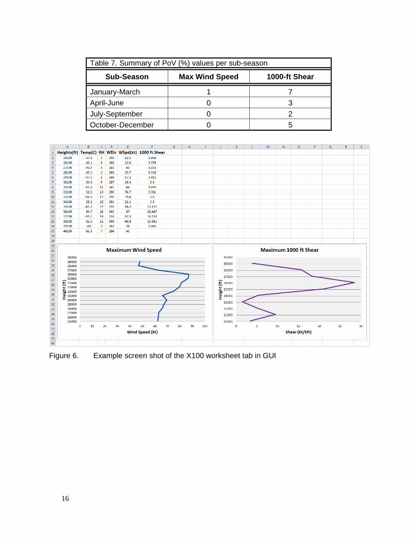
Table 7. Summary of PoV (%) values per sub-season .................................................................. 16
5
1. Introduction The 30th Operational Support Squadron Weather Flight (30 OSSWF) provides
comprehensive weather services to the space program at Vandenberg Air Force Base (VAFB) in California. One of their responsibilities is to monitor upper-level winds to ensure safe launch operations of the Minuteman III ballistic missile. The 30 OSSWF tasked the Applied Meteorology Unit (AMU) to analyze historical VAFB sounding data with the goal of determining the probability of violating (PoV) their upper-level thresholds for wind speed and shear constraints specific to this launch vehicle. The result is a tool that will replace their existing one, assist the 30 OSSWF Launch Weather Officers (LWOs) in determining the probability of exceeding specific wind threshold values, and improve the overall upper-level winds forecast.
6
2. Previous 30 OSSWF Operational Tool The 30 OSSWF provided the AMU with a Microsoft Excel spreadsheet containing their
current operational tool used for calculating wind shear and determining the likelihood of violating specific upper-level wind constraints. The AMU examined the contents of the file to determine how the values were calculated; it is important for the final tool to use the same equations as those used by the 30 OSSWF for consistent operational results. Some errors in the 30 OSSWF tool were discovered and the AMU informed the 30 OSSWF of the inconsistencies.
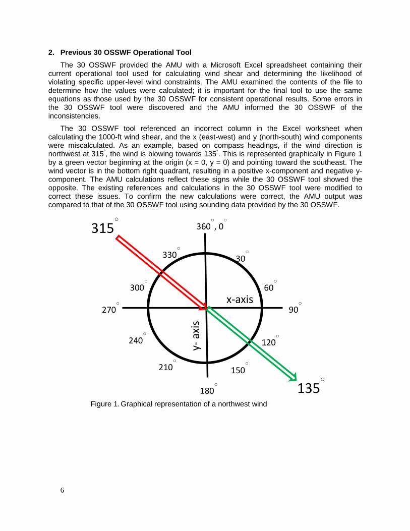
The 30 OSSWF tool referenced an incorrect column in the Excel worksheet when calculating the 1000-ft wind shear, and the x (east-west) and y (north-south) wind components were miscalculated. As an example, based on compass headings, if the wind direction is northwest at 315°, the wind is blowing towards 135°. This is represented graphically in Figure 1 by a green vector beginning at the origin (x = 0, y = 0) and pointing toward the southeast. The wind vector is in the bottom right quadrant, resulting in a positive x-component and negative y-component. The AMU calculations reflect these signs while the 30 OSSWF tool showed the opposite. The existing references and calculations in the 30 OSSWF tool were modified to correct these issues. To confirm the new calculations were correct, the AMU output was compared to that of the 30 OSSWF tool using sounding data provided by the 30 OSSWF.
Figure 1. Graphical representation of a northwest wind
y- a
xis
x-axis
360○, 0
○
30○
60○
90○
120○
150○
180○
210○
240○
270○
300○
330○
315○
135○
7
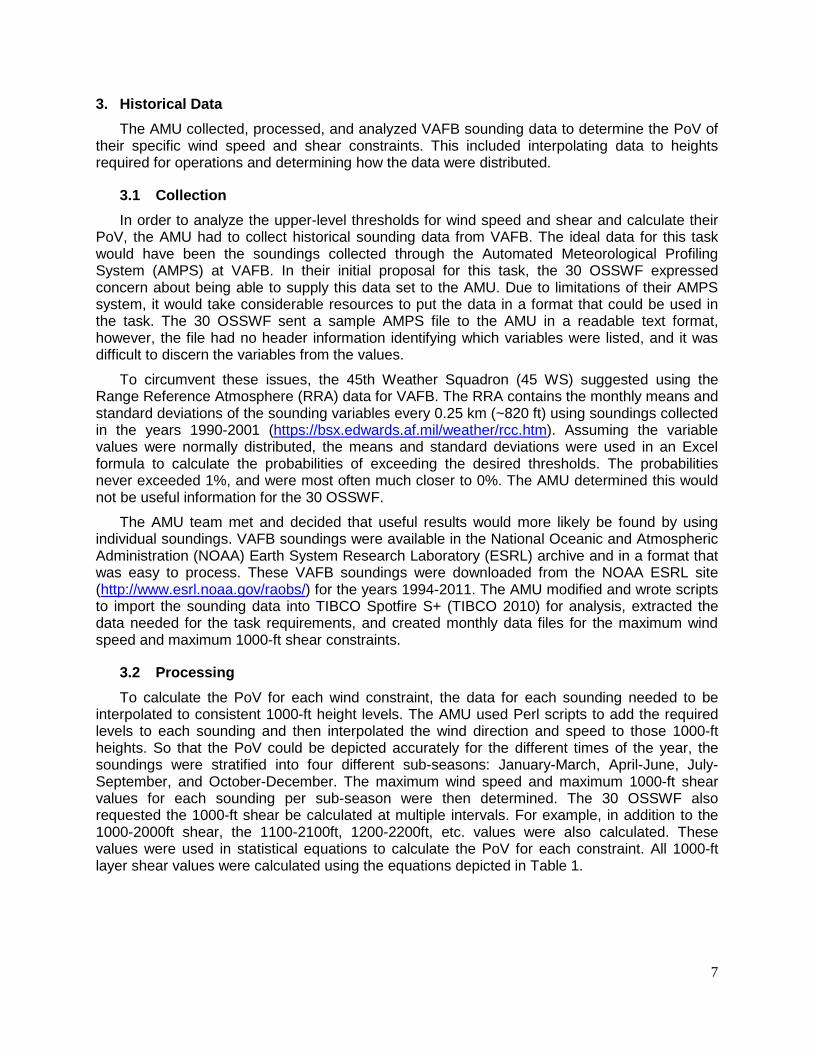
3. Historical Data The AMU collected, processed, and analyzed VAFB sounding data to determine the PoV of
their specific wind speed and shear constraints. This included interpolating data to heights required for operations and determining how the data were distributed.
3.1 Collection In order to analyze the upper-level thresholds for wind speed and shear and calculate their
PoV, the AMU had to collect historical sounding data from VAFB. The ideal data for this task would have been the soundings collected through the Automated Meteorological Profiling System (AMPS) at VAFB. In their initial proposal for this task, the 30 OSSWF expressed concern about being able to supply this data set to the AMU. Due to limitations of their AMPS system, it would take considerable resources to put the data in a format that could be used in the task. The 30 OSSWF sent a sample AMPS file to the AMU in a readable text format, however, the file had no header information identifying which variables were listed, and it was difficult to discern the variables from the values.
To circumvent these issues, the 45th Weather Squadron (45 WS) suggested using the Range Reference Atmosphere (RRA) data for VAFB. The RRA contains the monthly means and standard deviations of the sounding variables every 0.25 km (~820 ft) using soundings collected in the years 1990-2001 (https://bsx.edwards.af.mil/weather/rcc.htm). Assuming the variable values were normally distributed, the means and standard deviations were used in an Excel formula to calculate the probabilities of exceeding the desired thresholds. The probabilities never exceeded 1%, and were most often much closer to 0%. The AMU determined this would not be useful information for the 30 OSSWF.
The AMU team met and decided that useful results would more likely be found by using individual soundings. VAFB soundings were available in the National Oceanic and Atmospheric Administration (NOAA) Earth System Research Laboratory (ESRL) archive and in a format that was easy to process. These VAFB soundings were downloaded from the NOAA ESRL site (http://www.esrl.noaa.gov/raobs/) for the years 1994-2011. The AMU modified and wrote scripts to import the sounding data into TIBCO Spotfire S+ (TIBCO 2010) for analysis, extracted the data needed for the task requirements, and created monthly data files for the maximum wind speed and maximum 1000-ft shear constraints.
3.2 Processing To calculate the PoV for each wind constraint, the data for each sounding needed to be
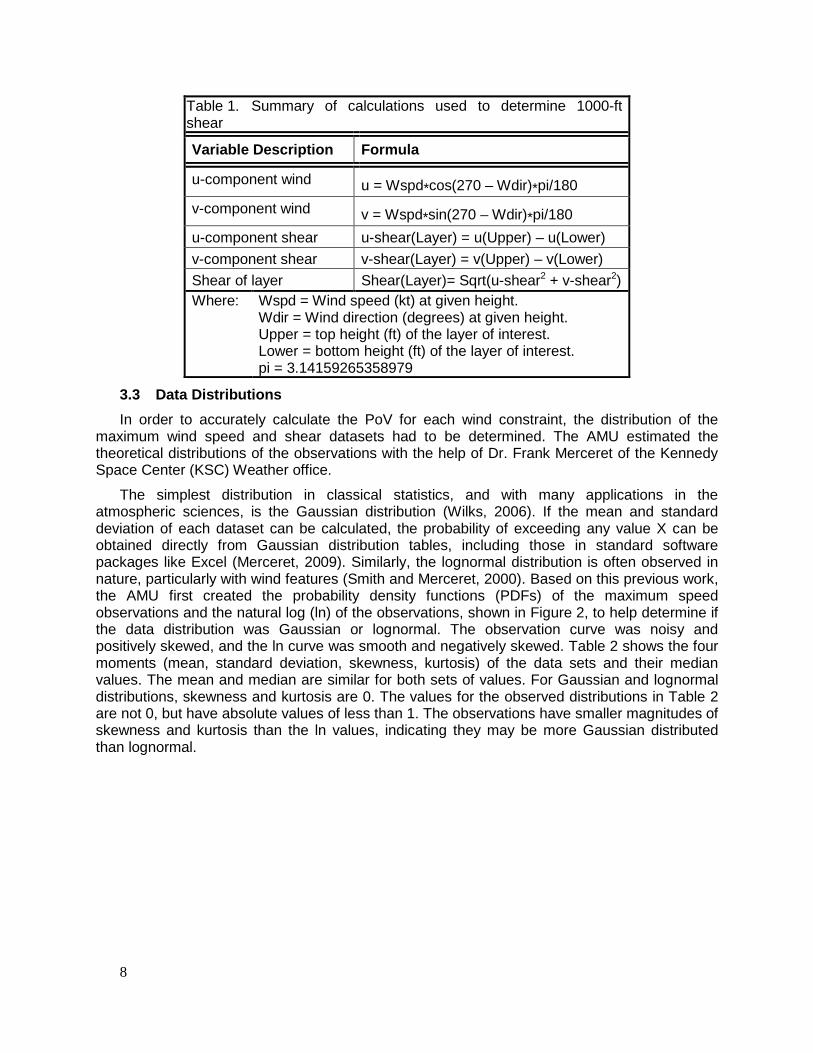
interpolated to consistent 1000-ft height levels. The AMU used Perl scripts to add the required levels to each sounding and then interpolated the wind direction and speed to those 1000-ft heights. So that the PoV could be depicted accurately for the different times of the year, the soundings were stratified into four different sub-seasons: January-March, April-June, July-September, and October-December. The maximum wind speed and maximum 1000-ft shear values for each sounding per sub-season were then determined. The 30 OSSWF also requested the 1000-ft shear be calculated at multiple intervals. For example, in addition to the 1000-2000ft shear, the 1100-2100ft, 1200-2200ft, etc. values were also calculated. These values were used in statistical equations to calculate the PoV for each constraint. All 1000-ft layer shear values were calculated using the equations depicted in Table 1.
Table 1. Summary of calculations used to determine 1000-ft shear
Variable Description Formula
u-component wind u = Wspd*cos(270 – Wdir)*pi/180 v-component wind v = Wspd*sin(270 – Wdir)*pi/180 u-component shear u-shear(Layer) = u(Upper) – u(Lower) v-component shear v-shear(Layer) = v(Upper) – v(Lower) Shear of layer Shear(Layer)= Sqrt(u-shear2 + v-shear2) Where: Wspd = Wind speed (kt) at given height.
Wdir = Wind direction (degrees) at given height. Upper = top height (ft) of the layer of interest. Lower = bottom height (ft) of the layer of interest. pi = 3.14159265358979
3.3 Data Distributions In order to accurately calculate the PoV for each wind constraint, the distribution of the
maximum wind speed and shear datasets had to be determined. The AMU estimated the theoretical distributions of the observations with the help of Dr. Frank Merceret of the Kennedy Space Center (KSC) Weather office.
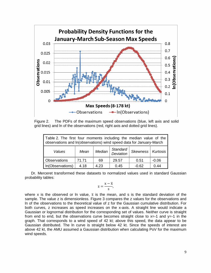
The simplest distribution in classical statistics, and with many applications in the atmospheric sciences, is the Gaussian distribution (Wilks, 2006). If the mean and standard deviation of each dataset can be calculated, the probability of exceeding any value X can be obtained directly from Gaussian distribution tables, including those in standard software packages like Excel (Merceret, 2009). Similarly, the lognormal distribution is often observed in nature, particularly with wind features (Smith and Merceret, 2000). Based on this previous work, the AMU first created the probability density functions (PDFs) of the maximum speed observations and the natural log (ln) of the observations, shown in Figure 2, to help determine if the data distribution was Gaussian or lognormal. The observation curve was noisy and positively skewed, and the ln curve was smooth and negatively skewed. Table 2 shows the four moments (mean, standard deviation, skewness, kurtosis) of the data sets and their median values. The mean and median are similar for both sets of values. For Gaussian and lognormal distributions, skewness and kurtosis are 0. The values for the observed distributions in Table 2 are not 0, but have absolute values of less than 1. The observations have smaller magnitudes of skewness and kurtosis than the ln values, indicating they may be more Gaussian distributed than lognormal.
9
Figure 2. The PDFs of the maximum speed observations (blue, left axis and solid grid lines) and ln of the observations (red, right axis and dotted grid lines).
Table 2. The first four moments including the median value of the observations and ln(observations) wind speed data for January-March
Values Mean Median Standard Deviation Skewness Kurtosis
Dr. Merceret transformed these datasets to normalized values used in standard Gaussian probability tables:
z =x − x�
s,
where x is the observed or ln value, x� is the mean, and s is the standard deviation of the sample. The value z is dimensionless. Figure 3 compares the z values for the observations and ln of the observations to the theoretical value of z for the Gaussian cumulative distribution. For both curves, z increases as speed increases on the x-axis. A straight line would indicate a Gaussian or lognormal distribution for the corresponding set of values. Neither curve is straight from end to end, but the observations curve becomes straight close to x=-1 and y=-1 in the graph. That corresponds to a wind speed of 42 kt; above this speed, the data appear to be Gaussian distributed. The ln curve is straight below 42 kt. Since the speeds of interest are above 42 kt, the AMU assumed a Gaussian distribution when calculating PoV for the maximum wind speeds.
10
Figure 3. Curves showing the relationship of the z values for the observations (blue) and the ln of the observations (red) to the theoretical Gaussian z values.
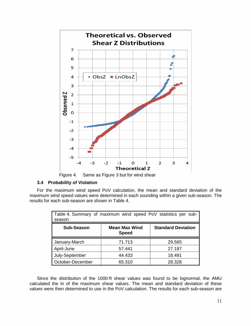
The AMU performed a similar analysis for the wind shear values. Table 3 shows the first four moments and median values for the two data sets. The values for the observations data set indicate it is not likely Gaussian distributed. The mean and median values are somewhat close, but skewness and kurtosis are far from 0. The values for ln of the observations are more indicative of a Gaussian distribution. The curve for the observations in Figure 4 is not straight at any point, but the ln curve becomes straight at x=-2.5 and y=-3 where the shear is 1.9 kt/1000 ft and remains quasi-straight through the point x=2.5 and y=2 where the shear value is 45 kt/1000 ft. The shear value of interest is well within the linear portion of the LN curve, leading the AMU to assume a lognormal distribution for the shear values.
Table 3. The first four moments including the median value of the observations and ln(observations) wind shear data for January-March.
Values Mean Median Standard Deviation Skewness Kurtosis
Since the distribution of the 1000-ft shear values was found to be lognormal, the AMU calculated the ln of the maximum shear values. The mean and standard deviation of these values were then determined to use in the PoV calculation. The results for each sub-season are
12
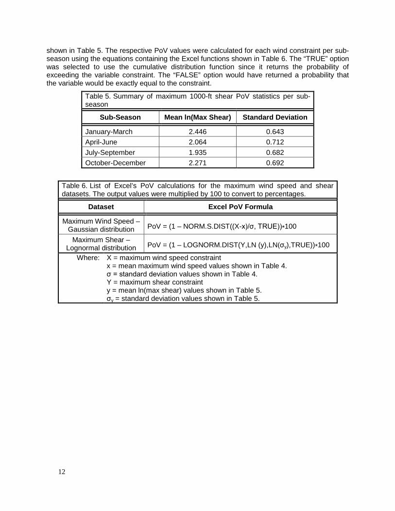
shown in Table 5. The respective PoV values were calculated for each wind constraint per sub-season using the equations containing the Excel functions shown in Table 6. The “TRUE” option was selected to use the cumulative distribution function since it returns the probability of exceeding the variable constraint. The “FALSE” option would have returned a probability that the variable would be exactly equal to the constraint.
Table 5. Summary of maximum 1000-ft shear PoV statistics per sub-season
Table 6. List of Excel’s PoV calculations for the maximum wind speed and shear datasets. The output values were multiplied by 100 to convert to percentages.
Dataset Excel PoV Formula
Maximum Wind Speed – Gaussian distribution PoV = (1 – NORM.S.DIST((X-x)/σ, TRUE))*100
Maximum Shear – Lognormal distribution PoV = (1 – LOGNORM.DIST(Y,LN (y),LN(σy),TRUE))*100
Where: X = maximum wind speed constraint x = mean maximum wind speed values shown in Table 4. σ = standard deviation values shown in Table 4. Y = maximum shear constraint y = mean ln(max shear) values shown in Table 5. σy = standard deviation values shown in Table 5.
13
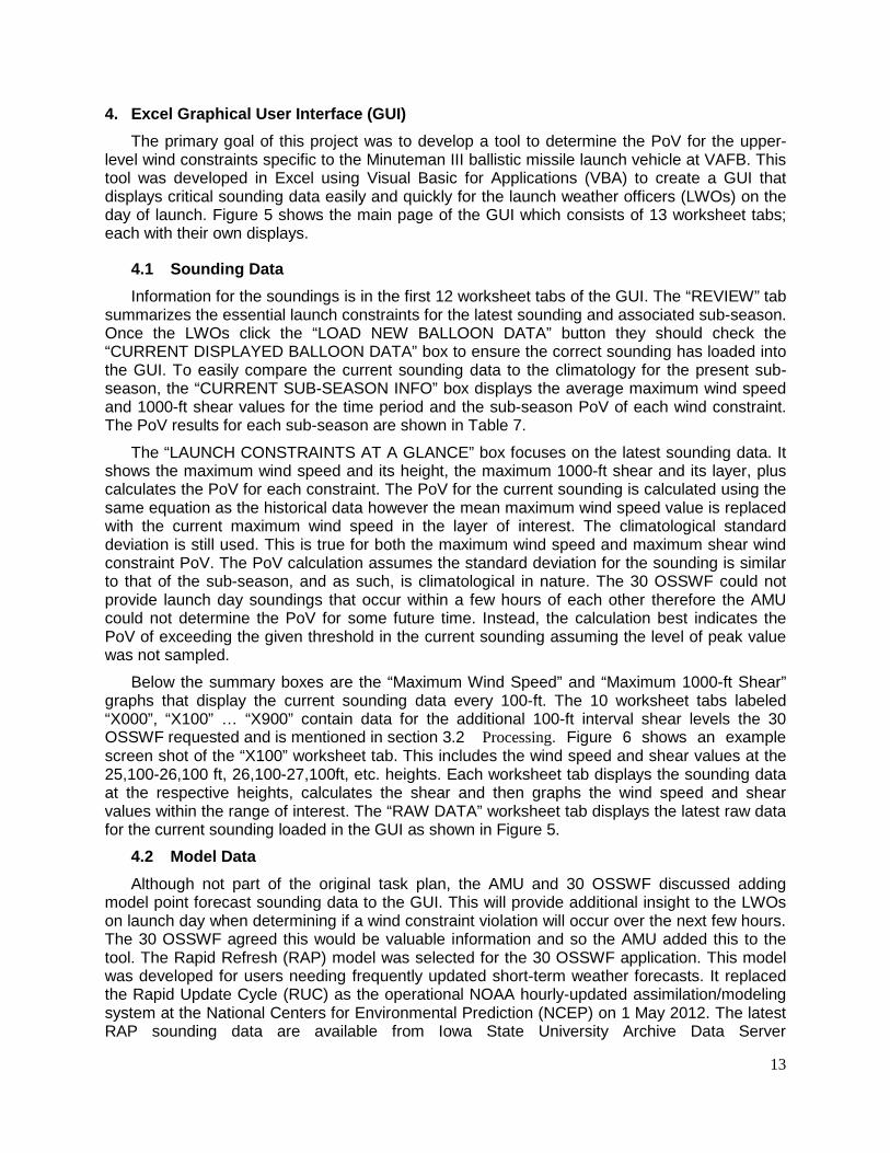
4. Excel Graphical User Interface (GUI) The primary goal of this project was to develop a tool to determine the PoV for the upper-
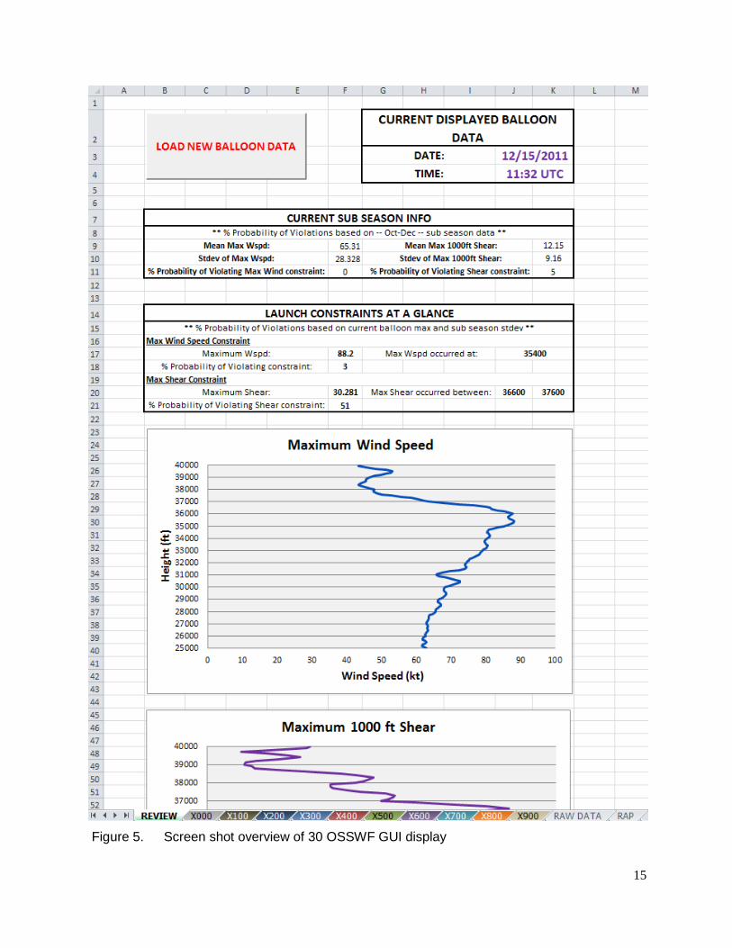
level wind constraints specific to the Minuteman III ballistic missile launch vehicle at VAFB. This tool was developed in Excel using Visual Basic for Applications (VBA) to create a GUI that displays critical sounding data easily and quickly for the launch weather officers (LWOs) on the day of launch. Figure 5 shows the main page of the GUI which consists of 13 worksheet tabs; each with their own displays.
4.1 Sounding Data Information for the soundings is in the first 12 worksheet tabs of the GUI. The “REVIEW” tab
summarizes the essential launch constraints for the latest sounding and associated sub-season. Once the LWOs click the “LOAD NEW BALLOON DATA” button they should check the “CURRENT DISPLAYED BALLOON DATA” box to ensure the correct sounding has loaded into the GUI. To easily compare the current sounding data to the climatology for the present sub-season, the “CURRENT SUB-SEASON INFO” box displays the average maximum wind speed and 1000-ft shear values for the time period and the sub-season PoV of each wind constraint. The PoV results for each sub-season are shown in Table 7.
The “LAUNCH CONSTRAINTS AT A GLANCE” box focuses on the latest sounding data. It shows the maximum wind speed and its height, the maximum 1000-ft shear and its layer, plus calculates the PoV for each constraint. The PoV for the current sounding is calculated using the same equation as the historical data however the mean maximum wind speed value is replaced with the current maximum wind speed in the layer of interest. The climatological standard deviation is still used. This is true for both the maximum wind speed and maximum shear wind constraint PoV. The PoV calculation assumes the standard deviation for the sounding is similar to that of the sub-season, and as such, is climatological in nature. The 30 OSSWF could not provide launch day soundings that occur within a few hours of each other therefore the AMU could not determine the PoV for some future time. Instead, the calculation best indicates the PoV of exceeding the given threshold in the current sounding assuming the level of peak value was not sampled.
Below the summary boxes are the “Maximum Wind Speed” and “Maximum 1000-ft Shear” graphs that display the current sounding data every 100-ft. The 10 worksheet tabs labeled “X000”, “X100” … “X900” contain data for the additional 100-ft interval shear levels the 30 OSSWF requested and is mentioned in section 3.2 Processing. Figure 6 shows an example screen shot of the “X100” worksheet tab. This includes the wind speed and shear values at the 25,100-26,100 ft, 26,100-27,100ft, etc. heights. Each worksheet tab displays the sounding data at the respective heights, calculates the shear and then graphs the wind speed and shear values within the range of interest. The “RAW DATA” worksheet tab displays the latest raw data for the current sounding loaded in the GUI as shown in Figure 5.
4.2 Model Data Although not part of the original task plan, the AMU and 30 OSSWF discussed adding
model point forecast sounding data to the GUI. This will provide additional insight to the LWOs on launch day when determining if a wind constraint violation will occur over the next few hours. The 30 OSSWF agreed this would be valuable information and so the AMU added this to the tool. The Rapid Refresh (RAP) model was selected for the 30 OSSWF application. This model was developed for users needing frequently updated short-term weather forecasts. It replaced the Rapid Update Cycle (RUC) as the operational NOAA hourly-updated assimilation/modeling system at the National Centers for Environmental Prediction (NCEP) on 1 May 2012. The latest RAP sounding data are available from Iowa State University Archive Data Server
14
(http://mtarchive.geol.iastate.edu) every hour and normally updated by 1hr and 45m after the hour. The “RAP” tab in the GUI displays two sounding graphs: one for wind speed and one for wind direction (See Figure 7). Each graph displays the respective variable for the current sounding profile plus 12 1-hour RAP forecast soundings. The RAP initialization time is based on the current UTC time.
Figure 6. Example screen shot of the X100 worksheet tab in GUI
17
Figure 7. Screen shot of the RAP tab in GUI
18
5. Summary and Future Work
The 30 OSSWF tasked the AMU to develop a tool that will calculate the PoV of the upper-level wind speed and shear constraints specific to the Minuteman III ballistic missile on the day of launch. In order to calculate each PoV, the AMU first collected historical sounding data from VAFB. The data were retrieved from the NOAA ESRL archive for the years 1994-2001 and stratified into four “sub-seasons” for analysis: January-March, April-June, July-September, and October-December. The maximum wind speed and 1000-ft shear values in increments of 100-ft for each sounding per sub-season were then determined. To accurately calculate the respective PoVs, the AMU determined the distribution of the maximum wind speed and maximum shear datasets by fitting these datasets with theoretical distributions. The AMU discovered that the maximum wind speeds followed a Gaussian distribution while the maximum shear values followed a lognormal distribution.
The AMU then developed a GUI in Excel using VBA that calculates the PoV for each wind constraint and displays current sounding data easily and quickly for the LWOs on launch day. In addition to the requirements outlined in the original task plan, the AMU also included forecast sounding data from the RAP model. This information provides further insight for the LWOs when determining if a wind constraint violation will occur over the next few hours. The AMU-developed tool will replace the existing one used by the 30 OSSWF, assist the LWOs in determining the probability of exceeding specific wind threshold values, and help to improve the overall upper-level winds forecast.
Another way to determine if a wind constraint violation will occur over the next few hours would be to conduct a statistical wind change study using 50 MHz wind profiler data similar to the calculations done in Merceret (1997). The results provided probabilities of exceeding a magnitude of wind vector change over 0.25, 1, 2 and 4 hours. The LWOs would determine what wind change between the last sounding and the launch time would pose an operational threat, then use pre-calculated values to determine the PoV of the constraint. The VAFB 50 MHz wind profiler is not yet functioning. Once it becomes operational, the AMU suggests that the data be archived in order to create these values for the 30 OSSWF.
19
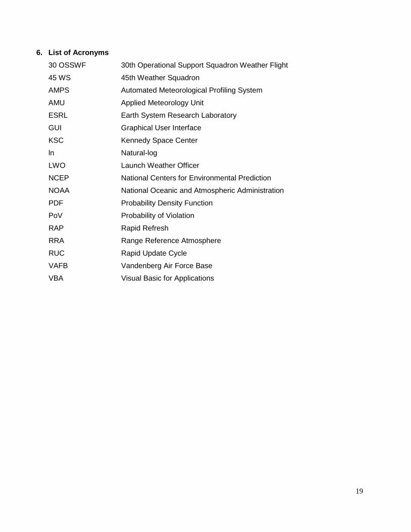
6. List of Acronyms 30 OSSWF 30th Operational Support Squadron Weather Flight
45 WS 45th Weather Squadron
AMPS Automated Meteorological Profiling System
AMU Applied Meteorology Unit
ESRL Earth System Research Laboratory
GUI Graphical User Interface
KSC Kennedy Space Center
ln Natural-log
LWO Launch Weather Officer
NCEP National Centers for Environmental Prediction
NOAA National Oceanic and Atmospheric Administration
PDF Probability Density Function
PoV Probability of Violation
RAP Rapid Refresh
RRA Range Reference Atmosphere
RUC Rapid Update Cycle
VAFB Vandenberg Air Force Base
VBA Visual Basic for Applications
20
7. References Merceret, F. J., 1997: Rapid temporal changes of midtropospheric winds. J. Appl. Meteor., 36,
1567-1575.
Merceret, F. J., 2009: Two empirical models for land-falling hurricane gust factors, National Weather Digest, 33(1), 27-36.
Smith, B. and F. J. Merceret, 2000: The lognormal distribution. College Math. J., 31, 259-261.
Wilks, D. S., 2006: Statistical Methods in the Atmospheric Sciences. 2nd ed. Academic Press, Inc., San Diego, CA, 88 pp.
21
NOTICE Mention of a copyrighted, trademarked or proprietary product, service, or document does not constitute endorsement thereof by the author, ENSCO Inc., the AMU, the National Aeronautics and Space Administration, or the United States Government. Any such mention is solely for the purpose of fully informing the reader of the resources used to conduct the work reported herein.