Page 1
Brigham Young University Brigham Young University
BYU ScholarsArchive BYU ScholarsArchive
Theses and Dissertations
2011-03-10
Variable Selection and Parameter Estimation Using a Continuous Variable Selection and Parameter Estimation Using a Continuous
and Differentiable Approximation to the L0 Penalty Function and Differentiable Approximation to the L0 Penalty Function
Douglas Nielsen VanDerwerken Brigham Young University - Provo
Follow this and additional works at: https://scholarsarchive.byu.edu/etd
Part of the Statistics and Probability Commons
BYU ScholarsArchive Citation BYU ScholarsArchive Citation VanDerwerken, Douglas Nielsen, "Variable Selection and Parameter Estimation Using a Continuous and Differentiable Approximation to the L0 Penalty Function" (2011). Theses and Dissertations. 2486. https://scholarsarchive.byu.edu/etd/2486
This Selected Project is brought to you for free and open access by BYU ScholarsArchive. It has been accepted for inclusion in Theses and Dissertations by an authorized administrator of BYU ScholarsArchive. For more information, please contact [email protected] , [email protected] .
Page 2
Variable Selection and Parameter Estimation using a Continuous and DifferentiableApproximation to the L0 Penalty Function
Douglas N. VanDerwerken
A project submitted to the faculty ofBrigham Young University
in partial fulfillment of the requirements for the degree of
Master of Science
H. Dennis Tolley, ChairDavid A. Engler
William F. Christensen
Department of Statistics
Brigham Young University
April 2011
Copyright c© 2011 Douglas N. VanDerwerken
All Rights Reserved
Page 4
ABSTRACT
Variable Selection and Parameter Estimation using a Continuous and DifferentiableApproximation to the L0 Penalty Function
Douglas N. VanDerwerkenDepartment of Statistics, BYU
Master of Science
L0 penalized likelihood procedures like Mallows’ Cp, AIC, and BIC directly penalizefor the number of variables included in a regression model. This is a straightforward ap-proach to the problem of overfitting, and these methods are now part of every statistician’srepertoire. However, these procedures have been shown to sometimes result in unstableparameter estimates as a result on the L0 penalty’s discontinuity at zero. One proposedalternative, seamless-L0 (SELO), utilizes a continuous penalty function that mimics L0 andallows for stable estimates. Like other similar methods (e.g. LASSO and SCAD), SELOproduces sparse solutions because the penalty function is non-differentiable at the origin.Because these penalized likelihoods are singular (non-differentiable) at zero, there is noclosed-form solution for the extremum of the objective function. We propose a continuousand everywhere-differentiable penalty function that can have arbitrarily steep slope in aneighborhood near zero, thus mimicking the L0 penalty, but allowing for a nearly closed-form solution for the β vector. Because our function is not singular at zero, β will haveno zero-valued components, although some will have been shrunk arbitrarily close thereto.We employ a BIC-selected tuning parameter used in the shrinkage step to perform zero-thresholding as well. We call the resulting vector of coefficients the ShrinkSet estimator. Itis comparable to SELO in terms of model performance (selecting the truly nonzero coeffi-cients, overall MSE, etc.), but we believe it to be more intuitive and simpler to compute. Weprovide strong evidence that the estimator enjoys favorable asymptotic properties, includingthe oracle property.
Keywords: Penalized likelihood; variable selection; oracle property; large p, small n
Page 6
ACKNOWLEDGMENTS
I would like to thank my advisor Dr. H. Dennis Tolley for proposing the ShrinkSet
penalty function and for his unrelenting insistence on rigor. In addition, I would like to
thank the other faculty members on my committee, especially Dr. David Engler, for their
helpful revisions. Many thanks also to Dr. Xihong Lin for her helpful comments and to Dr.
Valen Johnson for lending me R-code for the salary data analysis. Finally, I would like to
thank my wife, Charisse, for being supportive of me throughout this process, which included
many late nights in the Talmage building.
Page 8
CONTENTS
Contents . . . . . . . . . . . . . . . . . . . . . . . . . . . . . . . . . . . . . . . . . . vii
1 Introduction . . . . . . . . . . . . . . . . . . . . . . . . . . . . . . . . . . . . . . . 1
1.1 Outline . . . . . . . . . . . . . . . . . . . . . . . . . . . . . . . . . . . . . . . 2
2 Literature Review . . . . . . . . . . . . . . . . . . . . . . . . . . . . . . . . . . . . 3
2.1 Subset selection . . . . . . . . . . . . . . . . . . . . . . . . . . . . . . . . . . 4
2.2 Ridge regression . . . . . . . . . . . . . . . . . . . . . . . . . . . . . . . . . . 4
2.3 LASSO . . . . . . . . . . . . . . . . . . . . . . . . . . . . . . . . . . . . . . . 5
2.4 Bridge regression . . . . . . . . . . . . . . . . . . . . . . . . . . . . . . . . . 6
2.5 SCAD . . . . . . . . . . . . . . . . . . . . . . . . . . . . . . . . . . . . . . . 7
2.6 Adaptive LASSO . . . . . . . . . . . . . . . . . . . . . . . . . . . . . . . . . 8
2.7 SELO . . . . . . . . . . . . . . . . . . . . . . . . . . . . . . . . . . . . . . . 8
2.8 Other methods . . . . . . . . . . . . . . . . . . . . . . . . . . . . . . . . . . 9
3 Methods . . . . . . . . . . . . . . . . . . . . . . . . . . . . . . . . . . . . . . . . 11
3.1 Proposed penalty function . . . . . . . . . . . . . . . . . . . . . . . . . . . . 11
3.2 Iterative closed-form solution for our estimator . . . . . . . . . . . . . . . . . 13
3.3 Standard error formula . . . . . . . . . . . . . . . . . . . . . . . . . . . . . . 15
3.4 Selection of λ . . . . . . . . . . . . . . . . . . . . . . . . . . . . . . . . . . . 16
3.5 Selection of δ . . . . . . . . . . . . . . . . . . . . . . . . . . . . . . . . . . . 16
3.6 Oracle properties . . . . . . . . . . . . . . . . . . . . . . . . . . . . . . . . . 18
3.7 Application when p� n . . . . . . . . . . . . . . . . . . . . . . . . . . . . . 25
vii
Page 9
3.8 Other applications . . . . . . . . . . . . . . . . . . . . . . . . . . . . . . . . 27
4 Simulations and Results . . . . . . . . . . . . . . . . . . . . . . . . . . . . . . . 29
4.1 Estimator performance . . . . . . . . . . . . . . . . . . . . . . . . . . . . . . 29
4.2 Validation of Conjecture 1 . . . . . . . . . . . . . . . . . . . . . . . . . . . . 32
4.3 Simulations for large p, small n setting . . . . . . . . . . . . . . . . . . . . . 34
5 Data Analysis . . . . . . . . . . . . . . . . . . . . . . . . . . . . . . . . . . . . . 39
6 Conclusions and Further Research . . . . . . . . . . . . . . . . . . . . . . . . . . 43
Bibliography . . . . . . . . . . . . . . . . . . . . . . . . . . . . . . . . . . . . . . . . 45
viii
Page 10
chapter 1
INTRODUCTION
L0 penalized likelihood procedures like Mallows’ Cp, AIC, and BIC directly penalize for the
number of variables included in a regression model. This is a straightforward approach to
the problem of overfitting, and these methods are now part of every statistician’s repertoire.
However, Breiman (1996) demonstrates that these procedures can result in unstable param-
eter estimates. According to Dicker (2010), this instability is the result of the L0 penalty’s
discontinuity at zero. In addition, L0 likelihood procedures are generally NP-hard. In order
to improve computational efficiency over other methods and alleviate the instability prob-
lems identified by Breiman (1996), Dicker (2010) recommends “continuous penalty functions
designed to mimic the L0 penalty” and proposes one such penalty called the seamless-L0
(SELO). We go one step further and propose a continuous and differentiable penalty func-
tion that can have arbitrarily steep slope in a neighborhood near zero, thus mimicking the
L0 penalty, but allowing for a nearly closed-form solution for the β vector. The resulting
estimator is comparable to SELO in terms of model performance (selecting the truly nonzero
coefficients, overall MSE, etc.), but we believe it to be more intuitive and simpler to compute.
It has been shown (see Fan and Li (2001), Antoniadis and Fan (2001)) that a penalty
function cannot produce sparse solutions (solutions where many coefficients are estimated
to be zero) unless the penalty is singular at the origin. Because the proposed penalty
is differentiable at zero, it cannot produce sparse solutions on its own. However, due to
its arbitrarily steep slope in a neighborhood of the origin, the proposed penalty is able
to shrink estimates arbitrarily close to zero. We employ the same BIC-selected tuning
parameter to both shrink estimates towards zero and then threshold the shrunken estimates
to exactly zero. While our method at this point ceases to remain fully continuous, the
1
Page 11
amount of discontinuity is so small (because of the shrinkage step) that the major problems
with discontinuity identified by Breiman are averted. Importantly, the proposed estimator
appears to also enjoy asymptotic normality with the same asymptotic variance as the least
squares estimator. These properties (sparsity and asymptotic normality) comprise what Fan
and Li (2001) call the “oracle properties.” In other words, an oracle procedure performs as
well as if the set of truly nonzero coefficients were known in advance.
1.1 Outline
We first give a thorough discussion of the relevant literature on penalized likelihood meth-
ods. We then introduce the proposed penalty function and present an iterative closed-form
solution for β. We approximate the finite-sample distribution of the estimator, and establish
(through heuristic argument and simulation) its asymptotic oracle properties. We present
the results of various simulations and comment on various other applications of this method,
including where n � p. We conclude by analyzing a medical data set and a data set used
in a discrimination lawsuit. Throughout, we compare our method to standards in the field.
2
Page 12
chapter 2
LITERATURE REVIEW
Let X be an n × p data matrix where rows 1, . . . , n represent observations and columns
1, . . . , p represent variables. If an estimate for the intercept is desired, a column of 1’s may
be appended to X. The vector y is of length n and represents the response associated
with each observation. It is typically assumed that y follows a normal distribution with
expectation Xβ and variance σ2I when errors are independent, or more generally Σ. The
maximum likelihood estimator for β is β = (X′X)−1X′y. It is straightforward to show that
β is distributed normally with mean β and variance (X′X)−1σ2. Thus, the ordinary least
squares (OLS) estimator β is unbiased. Other advantages include that it has the minimum
variance of all unbiased estimators, that it is not computationally burdensome to calculate,
and that it is widely recognized and understood among other disciplines. In addition, it
is relatively easy to derive the OLS estimator’s finite-sample and asymptotic properties.
However, Hastie, Tibshirani, and Friedman (2009) point out two important drawbacks of β:
1. Prediction inaccuracy. Although β has zero bias, its variance can be high relative to
biased estimators. Shrinking or setting some coefficients to zero can improve overall
mean square error and prediction accuracy.
2. Interpretation. When p is high, it can be difficult to understand all effects simultane-
ously. Sometimes it may be advantageous to lose a little accuracy in exchange for a
more parsimonious model.
The following methods are meant to improve upon β in one or both of these areas.
3
Page 13
2.1 Subset selection
The idea of subset selection is to select the best subset (not necessarily proper) of the p
predictors of y in terms of some optimality criterion. The model chosen is the OLS estimator
fit on the X matrix of reduced dimensionality determined by those predictors which were
retained. Most optimality criteria directly penalize the number of terms in the model, thus
making use of the L0 penalty, and reward terms that are effective at reducing model error.
According to Dicker (2010), L0 penalties are of the form
pλ(βj) = λI{βj 6= 0},
where I is the indicator function. Examples of L0-based optimality criteria include Mallows’
Cp (Mallows 1973), AIC, (Akaike 1974), and BIC (Schwarz 1978). Breiman (1996) argues
that subset selection is unstable in that changing just one observation can drastically alter
the minimizer of the residual sum of squares. This is largely due to the all-or-nothing nature
of the L0 penalty. Less sophisticated methods such as choosing predictors so as to maximize
adjusted R2 or zero-thresholding coefficients with nonsignificant t-statistics are also meant
to reduce model size, but do not formally incorporate the L0 penalty.
2.2 Ridge regression
One of the first alternatives to ordinary least squares was ridge regression, which was de-
veloped by Hoerl and Kennard (1970) in order to deal with multicollinearity. The ridge
estimator is found by minimizing
Q(β) =n∑i=1
(yi − x′iβ
)2
+ λ
p∑j=1
β2j
with respect to β. In essence, the solution β minimizes the sum of squared residuals subject
top∑j=1
β2j ≤ f(λ),
4
Page 14
where f is a one-to-one function (Hastie et al. 2009). For λ > 0, Q(β) penalizes coefficients
based on their magnitude, where the amount of shrinkage is directly related to the choice of
λ. It is easily shown that
β = (X′X + λI)−1X′y
minimizes Q(β). Hoerl and Kennard (1970) introduced a graphic known as the “ridge
trace” to help the user determine the optimal value for λ. An important aspect of the
ridge shrinkage is that, in general, no coefficients are shrunk to exactly zero. Because ridge
regression does not shrink coefficients to zero, it is not really a variable selection technique.
We discuss it because it was one of the first attempts to gain popularity using an objective
function other than the sum of squared residuals. The other procedures presented below all
perform shrinkage of some coefficients to zero.
2.3 LASSO
LASSO, which stands for “least absolute shrinkage and selection operator,” was proposed
by Tibshirani (1996) as an alternative to subset selection and ridge regression that retains
the good features of both. Minimizing
Q(β) =n∑i=1
(yi − x′iβ
)2
+ λ
p∑j=1
|βj|
for a fixed value of λ with respect to β yields the LASSO estimate β. This is equivalent to
minimizing the sum of squared residuals subject to
p∑j=1
|βj| ≤ t,
where t ≥ 0 (or λ) is a tuning parameter that can be chosen by cross-validation, generalized
cross-validation, or “an analytical unbiased estimate of risk” (Tibshirani 1996). As in the
ridge case, increasing the tuning parameter leads to increased shrinkage. Unlike before, no
truly closed-form solution exists, though the iterative ridge regression algorithm
β(k+1)
= (X′X + λW)−1X′y,
5
Page 15
where W is a diagonal p × p matrix with diagonal elements |β(k)|−1, generally guarantees
convergence to the minimum of Q(β). Tibshirani (1996) offers several other algorithms for
finding β, but these were supplanted by the more efficient least angular regression (LARS)
algorithm in 2004 (Efron, Hastie, Johnstone, and Tibshirani 2004).
2.4 Bridge regression
Developed by Frank and Friedman (1993), bridge regression encompasses a large class of esti-
mators, of which subset selection, ridge, and LASSO are special cases. The bridge estimator
is found by minimizing:
Q(β) =n∑i=1
(yi − x′iβ
)2
+ λ
p∑j=1
|βj|γ
with respect to β where λ > 0 (as before) determines the strength of the penalty and γ > 0 is
an additional meta parameter that “controls the degree of preference for the true coefficient
vector β to align with the original variable axis directions in the predictor space” (Frank
and Friedman 1993). This is equivalent to minimizing the sum of squared residuals subject
top∑j=1
|βj|γ ≤ t
for some t, a function of λ. According to Fu (1998), Frank and Friedman (1993) did not
solve for the estimator of bridge regression for an arbitrary γ > 0, but they did recommend
optimizing the γ parameter. Fan and Li (2001) explain that the bridge regression solution
is only continuous for γ ≥ 1, but does not threshold (produce sparse solutions) when γ > 1.
Thus, only when γ = 1 (which is the LASSO penalty) is the solution continuous and sparse;
but then the solution is biased by a constant λ.
2.5 SCAD
The SCAD or “smoothly clipped absolute deviation” penalty was proposed by Fan and Li
(2001) in their seminal paper Variable Selection via Nonconcave Penalized Likelihood and
6
Page 16
its Oracle Properties. The SCAD penalty is best defined in terms of its first derivative,
p′λ(β) = λ
{I{β ≤ λ}+
(aλ− β)+(a− 1)λ
I{β > λ}},
where I is the indicator function. An important improvement of SCAD over LASSO is that
large values of β are penalized less than small values of β. Also, unlike traditional variable
selection procedures, the SCAD estimator’s sampling properties can be precisely established.
For example, Fan and Li (2001) demonstrated that as n increases, the SCAD procedure
selects the true set of nonzero coefficients with probability tending to one. In addition,
the SCAD estimator exhibits asymptotic normality with mean β and variance (X′X)−1σ2,
the variance with the true submodel known. These two properties — consistency in variable
selection (sometimes called “sparsity”) and asymptotic normality with the minimum possible
variance of an unbiased estimator — constitute the “oracle” properties. In other words, an
oracle procedure performs as well asymptotically as if the set of truly nonzero coefficients
were known in advance. Asymptotic oracle properties have become the gold standard in the
penalized likelihood literature. Finally, Fan and Li (2001) show that the SCAD penalty can
be effectively implemented in robust linear and generalized linear models.
2.6 Adaptive LASSO
LASSO was designed to retain the good features of subset selection (sparsity), and ridge
regression (continuity at zero, which leads to stable estimates). This it does, but at the cost
of producing asymptotically biased estimates because the penalty function is unbounded for
large βj. In addition, Zou (2006) proves that in nontrivial instances LASSO is inconsistent.
That is, in some cases it does not select, even asymptotically, the true set of nonzero coef-
ficients with probability tending to one. Therefore, LASSO was shown to not possess the
oracle properties. To remedy this problem, Zou (2006) proposes a weighted LASSO which
minimizes
Q(β) =n∑i=1
(yi − x′iβ
)2
+ λ
p∑j=1
wj|βj|.
7
Page 17
Zou (2006) suggests using wj = 1/|βj|γ, and calls the resulting estimator the adpative
LASSO. Optimal values of γ and λ can be found using two-dimensional cross-validation. The
minimum of Q(β) can be found efficiently using the LARS (Efron et al. 2004) algorithm since
the penalty function is convex. Importantly, for fixed p, as n increases, the adaptive LASSO
selects the true set of nonzero coefficients with probability tending to one. In addition,
the adaptive LASSO estimate exhibits asymptotic normality with mean β and variance
(X′X)−1σ2. Adaptive LASSO theory and methodology have been extended to generalized
linear models, where the oracle properties also hold.
2.7 SELO
The SELO or “seamless-L0” penalty was designed to mimic the L0 penalty without the jump
discontinuity. Proposed by Dicker (2010),
pSELO(βj, λ, τ) =λ
log(2)log
(|βj||βj|+ τ
+ 1
)utlizes a tuning parameter τ in addition to the λ parameter common in most penalized
likelihood procedures. When τ is small, pSELO(βj, λ, τ) ≈ λI{βj 6= 0}, yet because the
penalty is continuous, the L0 penalty’s inherent instability problems identified by Breiman
(1996) are mitigated. A recommended implementation fixes τ = 0.01, then maximizes the
penalized likelihood by a coordinate descent algorithm for a collection of λs, selecting the
optimal λ in terms of minimal BIC (Dicker 2010). (The LARS algorithm (Efron et al.
2004) could not be employed for optimization, because the SELO penalty is non-convex.)
Dicker (2010) shows through various simulations that in finite samples the SELO procedure
is superior to existing methods in terms of proportion of the time that the correct model
is selected, MSE, and model error (defined as (β − β)′Σ(β − β)). We shall use the same
simulation setup and criteria as Dicker (2010) to examine the finite-sample performance of
our estimator. Asymptotically, the SELO estimator enjoys the oracle properties described
by Fan and Li (2001).
8
Page 18
2.8 Other methods
The foregoing list is by no means exhaustive. It does, however, represent the most common
variable selection techniques based on penalized likelihood. Other variable selection methods
include the nonnegative garrote (Breiman 1995), the Dantzig selector (Candes and Tao 2007),
nonparametric methods (Doksum, Tang, and Tsui 2008), Bayesian methods (Mitchell and
Beauchamp 1988), the elastic net (Zou and Hastie 2005), neural networks (Wikel and Dow
1993), and random forests used for determining variable importance (Breiman 2001). In
addition, several authors have extended results for specific penalty functions to a broader
class of functions (see, for example, Fessler (1996), Antoniadis and Fan (2001), Fan and Li
(2001), or Antoniadis, Gijbels, and Nikolova (2009)).
9
Page 20
chapter 3
METHODS
3.1 Proposed penalty function
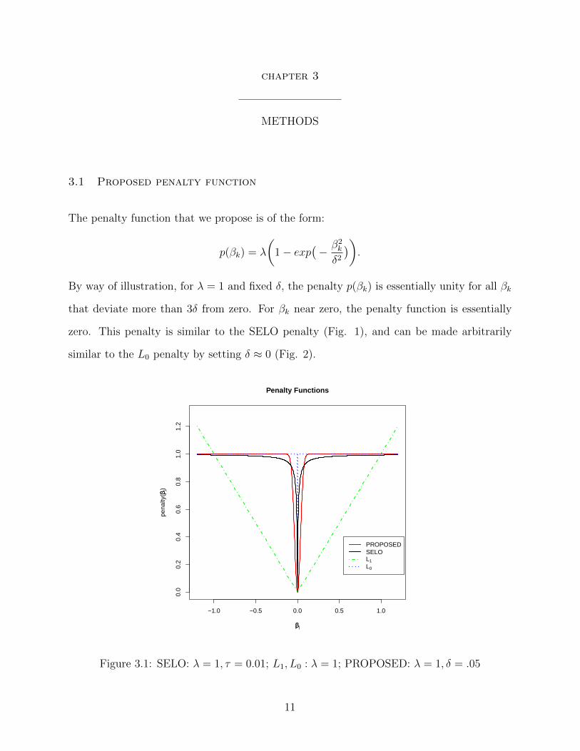
The penalty function that we propose is of the form:
p(βk) = λ
(1− exp
(− β2
k
δ2)).
By way of illustration, for λ = 1 and fixed δ, the penalty p(βk) is essentially unity for all βk
that deviate more than 3δ from zero. For βk near zero, the penalty function is essentially
zero. This penalty is similar to the SELO penalty (Fig. 1), and can be made arbitrarily
similar to the L0 penalty by setting δ ≈ 0 (Fig. 2).
−1.0 −0.5 0.0 0.5 1.0
0.0
0.2
0.4
0.6
0.8
1.0
1.2
Penalty Functions
ββj
pena
lty(ββ
j)
PROPOSEDSELOL1
L0
Figure 3.1: SELO: λ = 1, τ = 0.01; L1, L0 : λ = 1; PROPOSED: λ = 1, δ = .05
11
Page 21
In fact, it can be easily shown that the limit of p(βk) as δ2 → 0 is the L0 penalty. We state
this result as Theorem 1.
Theorem 1.
limδ2→0
pλ(βk) = λI{βk 6= 0},
where I is the indicator function.
Proof: Suppose βk 6= 0. Then limδ2→0
β2k
δ2=∞. Since limx→∞ e
−x = 0, we have limδ2→0 pλ(βk) =
λ. Now suppose βk = 0. By L’Hopital’s rule, we have limδ2→0β2k
δ2= 0. So limδ2→0 pλ(βk) =
λ(1− e0) = 0.
−1.0 −0.5 0.0 0.5 1.0
0.0
0.2
0.4
0.6
0.8
1.0
1.2
Limit of the Proposed Penalty Function
βj
pena
lty(β
j)
δ=0.4
δ=0.1
δ=0.005
PROPOSEDL0
Figure 3.2: L0 : λ = 1; PROPOSED: λ = 1 and δ varies. The limit of the proposed penalty
function as δ goes to zero is L0.
12
Page 22
We note that in their paper on categorizing classes of penalized likelihood penal-
ties, Antoniadis et al. (2009) refer to a slightly different form of p(βk) as an example of
a penalty function that is smooth at zero and non-convex. In addition, several papers on
image processing have cited this penalty function (sometimes called the Leclerc penalty) in
connection with shrinkage methods (e.g. Nikolova (2005), Corepetti, Heitz, Arroyo, Memin,
and Santa-Cruz (2006)). However, at the time of this writing, no attempt has been made in
the literature either to propose a method for obtaining an optimal value of δ, or to use this
penalty as the first step of a variable selection procedure, or to compare the associated sparse
estimator to established methods in terms of finite-sample or asymptotic performance, as
we do here.
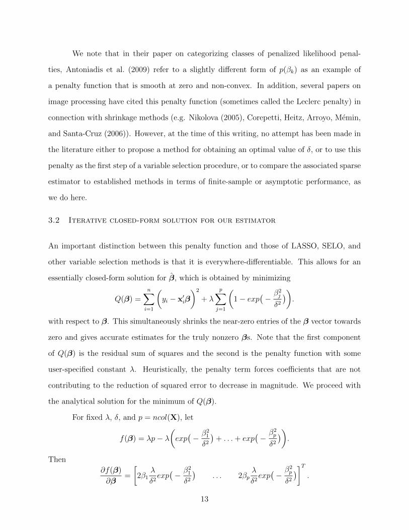
3.2 Iterative closed-form solution for our estimator
An important distinction between this penalty function and those of LASSO, SELO, and
other variable selection methods is that it is everywhere-differentiable. This allows for an
essentially closed-form solution for β, which is obtained by minimizing
Q(β) =n∑i=1
(yi − x′iβ
)2
+ λ
p∑j=1
(1− exp
(−β2j
δ2)).
with respect to β. This simultaneously shrinks the near-zero entries of the β vector towards
zero and gives accurate estimates for the truly nonzero βs. Note that the first component
of Q(β) is the residual sum of squares and the second is the penalty function with some
user-specified constant λ. Heuristically, the penalty term forces coefficients that are not
contributing to the reduction of squared error to decrease in magnitude. We proceed with
the analytical solution for the minimum of Q(β).
For fixed λ, δ, and p = ncol(X), let
f(β) = λp− λ(exp(− β2
1
δ2)
+ . . .+ exp(−β2p
δ2)).
Then
∂f(β)
∂β=
[2β1
λ
δ2exp(− β2
1
δ2)
. . . 2βpλ
δ2exp(−β2p
δ2)]T
.
13
Page 23
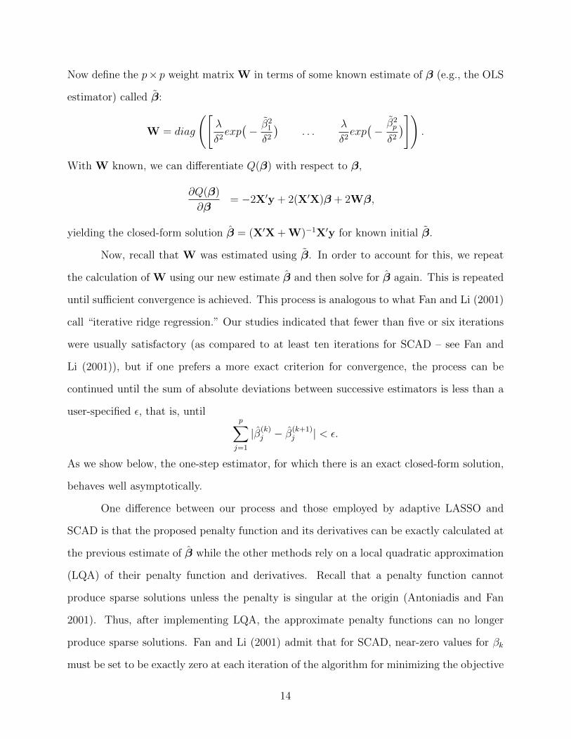
Now define the p× p weight matrix W in terms of some known estimate of β (e.g., the OLS
estimator) called β:
W = diag
([λ
δ2exp(− β2
1
δ2)
. . .λ
δ2exp(−β2p
δ2)])
.
With W known, we can differentiate Q(β) with respect to β,
∂Q(β)
∂β= −2X′y + 2(X′X)β + 2Wβ,
yielding the closed-form solution β = (X′X + W)−1X′y for known initial β.
Now, recall that W was estimated using β. In order to account for this, we repeat
the calculation of W using our new estimate β and then solve for β again. This is repeated
until sufficient convergence is achieved. This process is analogous to what Fan and Li (2001)
call “iterative ridge regression.” Our studies indicated that fewer than five or six iterations
were usually satisfactory (as compared to at least ten iterations for SCAD – see Fan and
Li (2001)), but if one prefers a more exact criterion for convergence, the process can be
continued until the sum of absolute deviations between successive estimators is less than a
user-specified ε, that is, untilp∑j=1
|β(k)j − β
(k+1)j | < ε.
As we show below, the one-step estimator, for which there is an exact closed-form solution,
behaves well asymptotically.
One difference between our process and those employed by adaptive LASSO and
SCAD is that the proposed penalty function and its derivatives can be exactly calculated at
the previous estimate of β while the other methods rely on a local quadratic approximation
(LQA) of their penalty function and derivatives. Recall that a penalty function cannot
produce sparse solutions unless the penalty is singular at the origin (Antoniadis and Fan
2001). Thus, after implementing LQA, the approximate penalty functions can no longer
produce sparse solutions. Fan and Li (2001) admit that for SCAD, near-zero values for βk
must be set to be exactly zero at each iteration of the algorithm for minimizing the objective
14
Page 24
function in order to “significantly reduce the computational burden.” Zou (2006) cites Fan
and Li’s LQA method when introducing adaptive LASSO, but fails to mention the implicit
zero-thresholding step. However, Zou and Li (2008), the (co-)authors of the adaptive LASSO
and SCAD papers, respectively, jointly wrote an article on one-step penalized likelihood
estimators, in which they are explicit about the fact that the zero-thresholding inherent in
LQA requires an additional tuning parameter (Zou and Li 2008).
Our method, on the other hand, can calculate the exact values of the penalty func-
tion and its derivatives at the previous estimate of β, because it is already everywhere-
differentiable. Because it is not singular at zero, it too must employ a zero-thresholding
tuning parameter. Recall that the proposed penalty is a function of λ and δ. These param-
eters must either be specified by the user or selected in terms of some optimality criterion.
The same tuning parameter δ can serve not only as an argument for the penalty function,
but also as a zero-thresholding cutoff to be used after our estimator converges to the mini-
mum of Q(β). Finding the minimum of Q(β) shrinks unimportant coefficients close to zero,
and then these coefficients can be set to be exactly zero, as in SCAD or adaptive LASSO.
We call it the ShrinkSet estimator to reflect this two-step process and because its function
as a variable selection technique is to reduce the dimensionality of our predictor space. The
method for choosing optimal values of λ and δ will be explained in more detail hereinafter.
3.3 Standard error formula
Letting A denote the set of indices corresponding to nonzero components of β, and for a fixed
matrix W, the vector βA is a linear combination of y. Thus, the exact variance-covariance
of βA, given W, is σ2(X′AXA+ WA,A)−1X′AXA(X′AXA+ WA,A)−1. Therefore, we estimate
the variance using the most recent estimate of W, called W:
V ar[βA
]= V ar
[βA|W
]= σ2(X′AXA + WA,A)−1X′AXA(X′AXA + WA,A)−1,
where σ2 = V ar [y] =(y −XAβA)′(y −XAβA)
(n− |A|)and |A| denotes the cardinality of A. This
corresponds nicely with the standard error estimates for adaptive LASSO, SCAD, and SELO
15
Page 25
obtained using a sandwich formula (see, for example, Tibshirani (1996)). Note that the limit
of V ar[βA
]as WA,A approaches the zero matrix is σ2(X′AXA)−1.
3.4 Selection of λ
The user specifies λ based on the perceived danger of overfitting. We would hope that a low
λ value would result in many nonzero βks and that a high λ value would allow only the most
extreme nonzero βks, as in LASSO. Because the ShrinkSet penalty is differentiable at zero,
however, it cannot shrink estimates to exactly zero, and so regardless of λ, the minimizer
of Q(β) retains all p coefficients. A reasonable surrogate, then, for the number of nonzero
parameters in the model, is
df(λ) = tr
(X(X′X + W(λ))−1X
),
which is monotone decreasing in λ (Hastie et al. 2009). If λ = 0, then df(λ) = p, and
the minimizer of Q(β) is the OLS estimator. Note that this corresponds nicely to the
interpretation of λ in the LASSO and ridge regression cases. Our studies suggest that after
zero-thresholding (discussed below), the resulting estimates β(λ) are similar across large
ranges of λ. Throughout this paper we use λ = 50, 000.
3.5 Selection of δ
Dicker (2010) cites several papers establishing the superiority of BIC tuning parameter
selection over GCV and AIC. Our simulations confirmed that in general BIC was a better
surrogate for MSE (prediction error) than was AIC or GCV. Following Dicker (2010), we
select the tuning parameter δ (for a fixed λ) so as to minimize
BIC(β) = log
[(y −Xβ)′(y −Xβ)
(n− d)
]+d× log(n)
n,
where d is the number of variables (nonzero coefficients) in the model.
Recall that everywhere-differentiable functions do not set any coefficients to exactly
zero. To produce sparse solutions using the ShrinkSet penalty, it is therefore necessary to
16
Page 26
employ a zero-thresholding function, which sets all components (of a vector-valued estimator)
to zero that do not exceed some threshold. A convenient choice for this threshold is δ. Thus
δ serves as a tuning parameter for the iterative ridge regression, which shrinks unimportant
βk towards zero, and as a zero-thresholding cutoff to be applied after said shrinkage. It turns
out that this thresholding after shrinkage is an important feature of our proposed variable
selection method. That the maximum penalized likelihood estimator (or its computationally
superior one-step surrogate) shrinks certain βk towards zero before employing the zero-
thresholding makes it superior to simply setting different sets of OLS coefficients to zero and
selecting the estimator with minimum BIC (see simulation studies section). This is equivalent
to running the ShrinkSet algorithm using λ = 0. The discontinuity discouraged by Breiman
(1996) is not so pronounced for relatively large λs, because the estimates are esentially
zero before they were set to be exactly zero. Also, unlike SCAD and adaptive LASSO, it
is not necessary to specify an additional tuning parameter, which can be computationally
burdensome.
In order to find the optimal δ, it was necessary to search over a dense grid of possible
values. The nature of the penalty function is such that δ ∈(0, max(|β|)
), but usually closer
to 0. We therefore begin our search over the range [ε, max(|β|)] for some user-specifed
ε > 0. A reasonable choice in many applications is ε = 0.005, or ε =1
2min(|β|). At each of
30 equally spaced δ values on this interval (endpoints included in the 30 values), we employ
the shrinking step by iteratively calculating β = (X′X+W(δ))−1X′y until convergence. We
then employ the zero-thresholding step by setting all βk < δ equal to zero. We calculate
BIC for each zero-thresholded β and find the δ associated with the minimum of the 30 BIC
values. Call this value δmin, and the δ values directly left and right of δmin call δL and
δR. We then narrow the search grid to [δL, δR] and calculate the thresholded estimate and
associated BIC at 30 equally spaced δ values in this range, including the endpoints. We
select as our optimal δ the value in the finer grid corresponding to the minimum BIC. We
found this approach to be more precise and more efficient than a dense search of the original
17
Page 27
range [ε, max(|β|)]. This is due to the relatively smooth, convex nature of the BIC curve
over this range. BIC(δ) will often have the same value for several values of δ in a small
range. This is because different choices for δ result in the same model. In these cases, we
select the smallest δ associated with the minimum BIC.
This procedure is one possible method for searching over a reasonably dense range of
δ values, but it can be easily adapted if the user desires more (or less) precision. For example,
in the p� n simulation studies, we elected to do a one-stage search over 30 equally spaced δ
values on[0.005,
1
4max(|β|)
]in order to save computation time. We found that regardless
of the setting the resulting estimator was largely invariant to the denseness of the δ-grid,
and the two-stage method described above was suitable for most applications.
3.6 Oracle properties
First recommended by Fan and Li (2001), procedures with the oracle properties have since
become the gold standard in the field of variable selection. The oracle properties are:
1. the procedure selects the truly nonzero βs and excludes the truly zero βs with proba-
bility tending to one as n increases, and
2. the nonzero components of the estimator are asymptotically normal about the true
nonzero β components with variance equal to the variance using OLS on the true
submodel.
More formally, let A denote the set of indices corresponding to truly nonzero components of
β, and let β be an estimator exhibiting the oracle properties. Then:
1. P (βA 6= 0) −→ 1 and P (βAc = 0) −→ 1 as n increases, and
2. βAd−→ N
(βA, (X
′AXA)−1σ2
).
18
Page 28
Let z(β, t) be a thresholding function that sets all components of β smaller than t in
(absolute value) to zero. That is, let
z(β, t) =
βk if |βk| ≥ t,
0 if |βk| < t.
Theorem 2.
For any threshold t such that 0 < t < min(|βA|
), there exists a pair (δ, λ) such that
z(β(δ, λ, β), t) selects the truly nonzero βs and excludes the truly zero-valued βs with prob-
ability tending to one. That is, there exists a pair such that:
limn→∞
P
(max
(|β
(1)
Ac |)< t < min
(|β
(1)
A |))
= 1.
Proof: Let t be such that 0 < t < min(|βA|
). Let i be the index corresponding to
max(|βAc|
)and let j be the index corresponding to min
(|βA|
). Consider the quotient
λ
δ2exp(−β2
j /δ2)
λ
δ2exp(−β2
i /δ2)
= exp
(β2i − β2
j
δ2
).
Note that:
limn→∞
P
(limδ2→0
exp
(β2i − β2
j
δ2
)=∞
)= 1,
because β is consistent which implies that the numerator of the exponent is asymptotically
positive in probability. However, for fixed λ,
limn→∞
P
(limδ2→0
λ
δ2exp(−β2
j /δ2) = 0
)= 1
and
limn→∞
P
(limδ2→0
λ
δ2exp(−β2
i /δ2) = 0
)= 1,
so
limn→∞
P
(limδ2→0
W(δ, λ, β) = [0]
)= 1.
19
Page 29
Instead of W = [0] (yielding β = (X′X + W)−1X′y = β and consequently no shrinkage),
we would prefer W to have high values on diagonal elements corresponding to zero-valued
β components, and near-zero values on diagonal elements corresponding to nonzero β com-
ponents. Note that in the ideal (but impossible) scenario, we would have:
Wp×p =
w1,1 0 · · · 0
0 w2,2 · · · 0
......
. . ....
0 0 · · · wp,p
,
where wA,A = 0 and wAc,Ac =∞. This would yield the solution
β =
βj if j ∈ A,
0 if j ∈ Ac,
which has the oracle properties. We show that min(WA,A) can be arbitrarily high in prob-
ability, while max(WAc,Ac) can be arbitrarily small (close to zero) in probability.
Choose M large enough and ε > 0 small enough that
β = (X′X + W)−1X′y ≈
βj if j ∈ A,
0 if j ∈ Ac
for
Wp×p =
w1,1 0 · · · 0
0 w2,2 · · · 0
......
. . ....
0 0 · · · wp,p
,
where max(wA,A) < ε and min(wAc,Ac) > M . Fix ε∗ > 0. From above, it is possible to
choose an n large enough and a δ2 small enough that
P
(exp( β2
i − β2j
δ2)>M
ε
)> 1− ε∗.
20
Page 30
For these values of n and δ2, we shall define λ =M + 1
1
δ2exp(−β2
j /δ2)
. Note that
λ
δ2exp(−β2
j /δ2)
λ
δ2exp(−β2
i /δ2)
= exp
(β2i − β2
j
δ2
)>M
ε
(with arbitrarily high probability), whileλ
δ2exp(−β2
j /δ2) > M , and
λ
δ2exp(−β2
i /δ2) < ε
(again, with arbitrarily high probability). Therefore,
β = (X′X + W)−1X′y ≈
βj if j ∈ A,
0 if j ∈ Ac
and the approximation can be as exact as desired (with arbitrarily high probability). More
specifically, the approximation can be exact enough that for any t such that 0 < t <
min(|βA|),
max(|β
(1)
Ac |)< t < min
(|β
(1)
A |)
with arbitrarily high probability. Therefore, for any t > 0, there exists a pair (δ, λ) such
that z(β(δ, λ, β), t) selects the truly nonzero βs and excludes the truly zero-valued βs with
probability tending to one.
We have proved that it is possible to shrink estimates in one step such that the largest
near-zero coefficient is arbitrarily small, and the smallest “nonzero” coefficient is arbitrarily
close to the corresponding the OLS-estimated coefficient. It is important however, that we
extend this theory to k-step estimator.
Conjecture 1.
Given a data set with n sufficiently large and fixed p, assume we have a pair (δ, λ) meeting
the criteria of Theorem 2. Then z(β(1), δ)
p−→ β.
Proof: (Outline) We know that βp−→ β, by the consistency of the OLS estimator.
This allowed us to establish that there exists a pair (δ, λ) such that z(β(1), δ)Ac = 0 and
21
Page 31
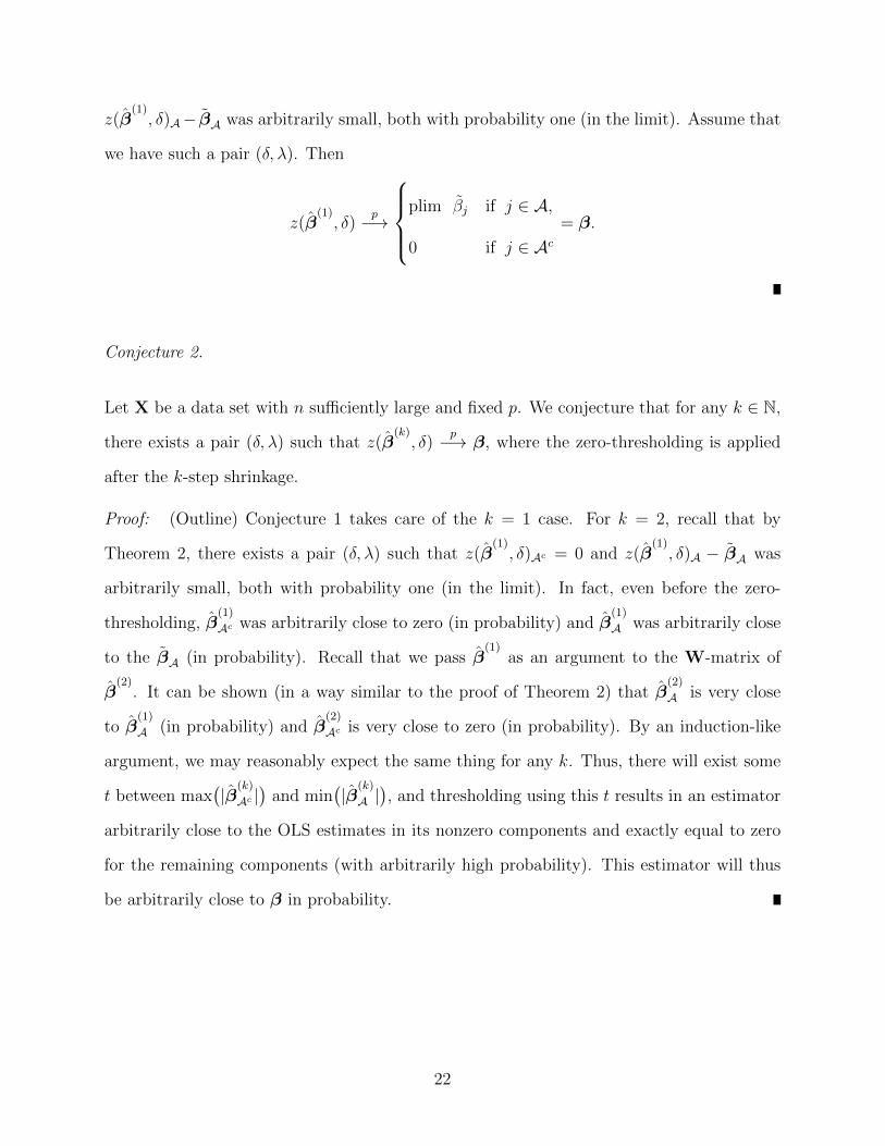
z(β(1), δ)A− βA was arbitrarily small, both with probability one (in the limit). Assume that
we have such a pair (δ, λ). Then
z(β(1), δ)
p−→
plim βj if j ∈ A,
0 if j ∈ Ac= β.
Conjecture 2.
Let X be a data set with n sufficiently large and fixed p. We conjecture that for any k ∈ N,
there exists a pair (δ, λ) such that z(β(k), δ)
p−→ β, where the zero-thresholding is applied
after the k-step shrinkage.
Proof: (Outline) Conjecture 1 takes care of the k = 1 case. For k = 2, recall that by
Theorem 2, there exists a pair (δ, λ) such that z(β(1), δ)Ac = 0 and z(β
(1), δ)A − βA was
arbitrarily small, both with probability one (in the limit). In fact, even before the zero-
thresholding, β(1)
Ac was arbitrarily close to zero (in probability) and β(1)
A was arbitrarily close
to the βA (in probability). Recall that we pass β(1)
as an argument to the W-matrix of
β(2)
. It can be shown (in a way similar to the proof of Theorem 2) that β(2)
A is very close
to β(1)
A (in probability) and β(2)
Ac is very close to zero (in probability). By an induction-like
argument, we may reasonably expect the same thing for any k. Thus, there will exist some
t between max(|β
(k)
Ac |)
and min(|β
(k)
A |), and thresholding using this t results in an estimator
arbitrarily close to the OLS estimates in its nonzero components and exactly equal to zero
for the remaining components (with arbitrarily high probability). This estimator will thus
be arbitrarily close to β in probability.
22
Page 32
Conjecture 3.
The proposed method of fixing λ and finding δ2 using t = δ and BIC will obtain a pair (λ, δ)
meeting the criteria of Theorem 2 and Conjecture 2 with probability tending to one as n
increases.
Proof: (Outline) We provide a heuristic argument for this conjecture. BIC has been shown
to be asymptotically consistent in a number of penalized likelihood model selection settings
as long as the true sparse model is among the candidate models (e.g. Dicker (2010), Zou,
Hastie, and Tibshirani (2007), Wang, Li, and Tsai (2007), and their references). For large
enough n, by searching over a range of zero-thresholding δ values, we essentially guarantee
that the true model will be among the candidate models. Thus, it is reasonable to suspect
that BIC will be consistent for model selection in this setting. Note that BIC being consistent
in this setting is equivalent to the pair (δmin(BIC), λ) meeting the criteria of Theorem 2 and
Conjecture 2.
The implication of Theorem 2 and Conjectures 1-3 is that the estimator obtained
using the described thresholding rule, z(β(β, δ, λ)(k), δ), will possess the oracle properties
for any k. This is due to the two-step nature of the ShrinkSet estimator, which shrinks the
near-zero estimates very close to zero and then sets them to zero. The coefficients far from
zero experience little shrinkage and mimic their corresponding OLS coefficients. We state
the oracle property implication formally in Theorem 3.
Theorem 3.
If Conjectures 2-3 hold, then the proposed k-step ShrinkSet estimator possess the oracle
properties for any k ∈ N .
Proof: By Conjecture 3, the proposed method of fixing λ and finding δ2 using t = δ
and BIC will obtain a pair (λ, δ) meeting the criteria of Conjecture 2. By Conjecture 2,
z(β(k), δ)
p−→ β for any k ∈ N .
23
Page 33
In the nonzero components of β, z(β(k), δ) converges in probability to β by virtue of
β(k)
’s arbitrary nearness to β. So, asymptotically, β(k)
A will have the same distribution as the
OLS estimator: it will be normally distributed with mean βA and variance (X′AXA)−1σ2.
In the zero-valued components of β, z(β(k), δ) converges in probability to β by
virtue of the thresholding rule. Since P(|β(k)i | < δ
), where i is the index corresponding
to max(|β
(k)
Ac |), approaches one asymptotically, the ShrinkSet estimator selects the truly
nonzero βs and excludes the truly zero-valued βs with probability tending to one.
In the simulation section, we show that δmin(BIC) tends to zero in probability, but
not as fast as the largest should-be-zero coefficients. Furthermore, we demonstrate that
as n increases, P(max(|β
(1)
Ac |) < δ)
approaches 1, thus showing that the requirements of
Theorem 2 have been met. We then demonstrate that for high n, the one-step ShrinkSet
procedure results in approximately normal estimators, with mean equal to the true β value
and variance approximately equal to that of the OLS estimator. This further establishes
the tenability of Conjectures 1-3, which, when combined with Theorem 2, imply that the
ShrinkSet estimators will possess the oracle properties.
3.7 Application when p� n
An important application of variable selection procedures is when there are many more
variables measured on each individual than there are individuals in the study, the so-called
“large p, small n” problem. For example, genomic data can have thousands of variables
collected on a few dozen patients. We describe two possible implementations of our approach
and compare these to two LASSO-based models built using glmnet (Friedman, Hastie, and
Tibshirani 2010). We do not include SELO in our comparison, because Dicker (2010) has
not extended the results to the p � n setting. In both ShrinkSet implementations, and
for the first LASSO model, we select the estimator which minimizes a BIC-type parameter
(called “extended BIC” (EBIC)), adapted for high-dimensional analysis. Following Lian
24
Page 34
(2010) closely, we minimize
EBIC(β) = log
[(y −Xβ)′(y −Xβ)
n
]+d · log(n)
√p
n.
Although Lian (2010) employs EBIC for high-dimensional varying coefficient models based
on B-spline basis expansions, our results suggest that their method can be used effectively
in simpler settings. For comparison, we also include a LASSO model selected by minimum
cross-validation error. We shall include two simulation scenarios: one with 7 nonzero coeffi-
cients out of p = 10, 000 with moderate covariance, and one with 16 nonzero coefficients out
of p = 1, 000 with very high covariance.
Implementation 1: Reducing X matrix in terms of correlation with y
Because our estimate is based on the X′X matrix, it is impossible to reliably estimate p > n
truly nonzero βs. However, if we constrain some of these estimates to be zero (which our
method does automatically), then we can produce reliable estimates of some subset of less
than n coefficients. We observed that choosing p < .85n columns of X was typically more
effective than choosing p < n. Therefore, we begin by selecting one at a time the .85n
columns of X most highly correlated with y. We redefine X as only those columns of X
and run our algorithm. This is very similar to the sure independence screening procedure
recommended by Fan and Lv (2008). In the results section, we call this the correlation
method.
Implementation 2: Reducing X matrix based on LASSO output
A dimension-reduction alternative is to use output from LASSO itself. We overfit a LASSO
model using glmnet with small λ and keep only those columns of X corresponding to nonzero
βs. If this is larger than .85n, we reduce further in terms of correlation with y, until we
have less than p ≤ .85n We then run our algorithm to shrink “nonsignificant” βs to zero.
We call this the hybrid method.
25
Page 35
LASSO with λ selected by EBIC
Using glmnet (Friedman et al. 2010), we obtain 100 different βs, each vector corresponding
to a different value of λ. We choose the model with the minimum EBIC.
LASSO with λ selected by cross-validation
Using cv.glmnet (Friedman et al. 2010), we find the value of λ associated with the minimum
cross-validation error. We then fit a LASSO model by passing this λ value as an argument
to glmnet (Friedman et al. 2010). We use leave-one-out cross-validation in the p = 1, 000
case and 10-fold cross-validation in the p = 10, 000 case.
3.8 Other applications
Robust regression
The least squares estimate is not robust against outliers, and nor is our proposed estimator,
because it relies on penalized least squares. However, if we use an outlier-resistant loss
function, such as Huber’s ψ function (Huber 1964), and minimize
Q(β) =n∑i=1
ψ(|yi − x′iβ|) + λ
p∑j=1
(1− exp
(−β2j
δ2)),
as suggested by Fan and Li (2001) (but with a different penalty), the result will be a robust
estimator, with nonsignificant terms shrunk to zero after the zero-thresholding step. We
suspect that a solution for this optimization is possible using iteratively reweighted least
squares, as shown by Fan and Li (2001), but with appropriate modification of the weights.
Link functions
Our method can also be generalized so as to accommodate different link functions such as
log, logit, and probit. For example, modifying a result by Zou (2006), the penalized logistic
26
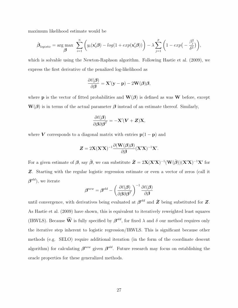
Page 36
maximum likelihood estimate would be
βlogistic = arg maxβ
n∑i=1
(yi(x
′iβ)− log(1 + exp(x′iβ))
)− λ
p∑j=1
(1− exp
(−β2j
δ2)),
which is solvable using the Newton-Raphson algorithm. Following Hastie et al. (2009), we
express the first derivative of the penalized log-likelihood as
∂`(β)
∂β= X′(y − p)− 2W(β)β,
where p is the vector of fitted probabilities and W(β) is defined as was W before, except
W(β) is in terms of the actual parameter β instead of an estimate thereof. Similarly,
∂`(β)
∂β∂βT= −X′(V +Z)X,
where V corresponds to a diagonal matrix with entries p(1− p) and
Z = 2X(X′X)−1∂(W(β)β)
∂β(X′X)−1X′.
For a given estimate of β, say β, we can substitute Z = 2X(X′X)−1(W(β))(X′X)−1X′ for
Z. Starting with the regular logistic regression estimate or even a vector of zeros (call it
βold), we iterate
βnew = βold −(∂`(β)
∂β∂βT
)−1∂`(β)
∂β
until convergence, with derivatives being evaluated at βold and Z being substituted for Z.
As Hastie et al. (2009) have shown, this is equivalent to iteratively reweighted least squares
(IRWLS). Because W is fully specified by βold, for fixed λ and δ our method requires only
the iterative step inherent to logistic regression/IRWLS. This is significant because other
methods (e.g. SELO) require additional iteration (in the form of the coordinate descent
algorithm) for calculating βnew given βold. Future research may focus on establishing the
oracle properties for these generalized methods.
27
Page 38
chapter 4
SIMULATIONS AND RESULTS
4.1 Estimator performance
Setup
We use the same simulation parameters as in Dicker (2010). That is, we set y = Xβ + ε
where X ∼ N(0,Σ), β = (3, 1.5, 0, 0, 2, 0, 0, 0)T , and ε ∼ N(0, σ2); we took Σ = (σij), where
σij = .5|i−j|; each simulation consisted of the generation of 1,000 independent data sets and
parameter estimation for each data set; four simulations were conducted: all combinations of
n ∈ {50, 100} and σ2 ∈ {1, 9}. Metrics observed at each iteration of the simulations include:
1. whether the correct set of nonzero coefficients was selected,
2. the average model size (number of nonzero coefficients),
3. the mean squared error,||β − β||2
p, and
4. the model error, (β − β)TΣ(β − β).
All simulations in this paper were performed on a Mac OS X (Version 10.5.8) with a 2.66
GHz Intel Core 2 Duo processor.
One drawback we see in some of the literature on variable selection is a neglect to
fairly compare the proposed method to OLS. For example, Dicker (2010) asserts that OLS
does not perform variable selection and proceeds to compare its performance in model size
to those of variable selection methods without any attempt to pare down the OLS model. A
fairer approach would be to include some automated OLS-based variable selection method,
like a stepwise selection procedure or even regular OLS with all nonsignificant (α = 0.05,
29
Page 39
for example) estimates set to zero. In the next section we present our proposed method’s
results, along with those of Dicker (2010) for reference. We also include OLS results where
nonsignificant estimates were estimated to be zero.
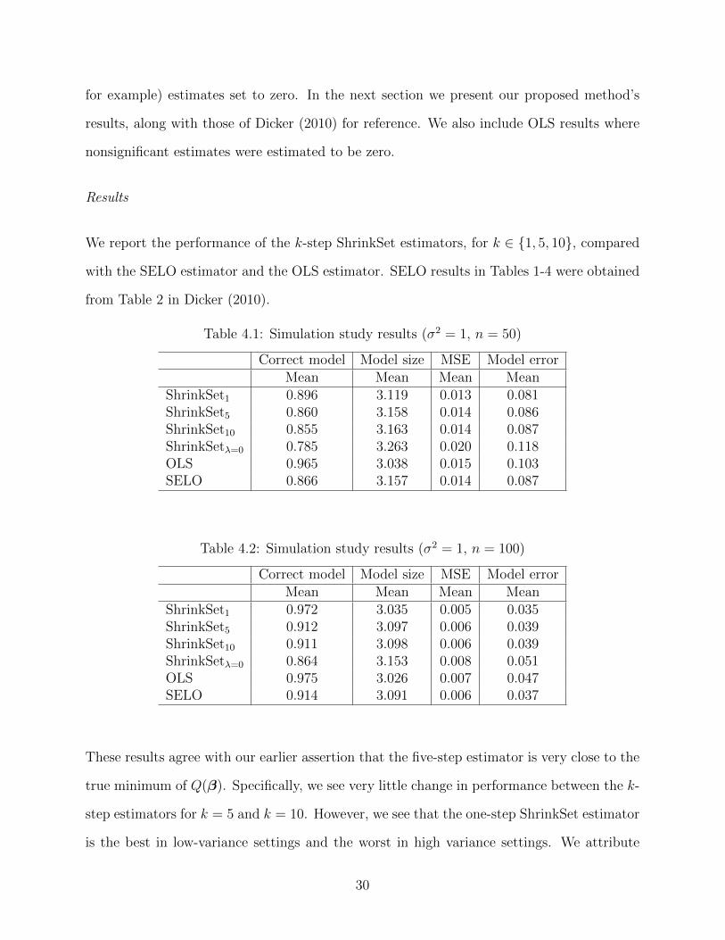
Results
We report the performance of the k-step ShrinkSet estimators, for k ∈ {1, 5, 10}, compared
with the SELO estimator and the OLS estimator. SELO results in Tables 1-4 were obtained
from Table 2 in Dicker (2010).
Table 4.1: Simulation study results (σ2 = 1, n = 50)
Correct model Model size MSE Model errorMean Mean Mean Mean
ShrinkSet1 0.896 3.119 0.013 0.081ShrinkSet5 0.860 3.158 0.014 0.086ShrinkSet10 0.855 3.163 0.014 0.087ShrinkSetλ=0 0.785 3.263 0.020 0.118OLS 0.965 3.038 0.015 0.103SELO 0.866 3.157 0.014 0.087
Table 4.2: Simulation study results (σ2 = 1, n = 100)
Correct model Model size MSE Model errorMean Mean Mean Mean
ShrinkSet1 0.972 3.035 0.005 0.035ShrinkSet5 0.912 3.097 0.006 0.039ShrinkSet10 0.911 3.098 0.006 0.039ShrinkSetλ=0 0.864 3.153 0.008 0.051OLS 0.975 3.026 0.007 0.047SELO 0.914 3.091 0.006 0.037
These results agree with our earlier assertion that the five-step estimator is very close to the
true minimum of Q(β). Specifically, we see very little change in performance between the k-
step estimators for k = 5 and k = 10. However, we see that the one-step ShrinkSet estimator
is the best in low-variance settings and the worst in high variance settings. We attribute
30
Page 40
Table 4.3: Simulation study results (σ2 = 9, n = 50)
Correct model Model size MSE Model errorMean Mean Mean Mean
ShrinkSet1 0.560 2.891 0.252 1.378ShrinkSet5 0.597 2.897 0.242 1.305ShrinkSet10 0.602 2.898 0.241 1.301ShrinkSetλ=0 0.565 3.025 0.254 1.524OLS 0.287 2.132 0.419 3.188SELO 0.605 2.913 0.240 1.310
Table 4.4: Simulation study results (σ2 = 9, n = 100)
Correct model Model size MSE Model errorMean Mean Mean Mean
ShrinkSet1 0.852 3.059 0.075 0.436ShrinkSet5 0.864 3.066 0.071 0.419ShrinkSet10 0.867 3.065 0.070 0.416ShrinkSetλ=0 0.820 3.148 0.084 0.522OLS 0.780 2.839 0.116 0.804SELO 0.879 3.061 0.070 0.408
the varying success of the one-step ShrinkSet estimator to its direct reliance on the OLS
estimator. We find it noteworthy that Dicker (2010) observed a similar phenomenon for the
SELO one-step estimator. In all scenarios, the five-step and ten-step ShrinkSet estimators
tend to be very similar to the SELO estimator. Importantly, these ShrinkSet estimators
outperform the λ = 0 estimator across the board, which shows that the shrinkage step is
crucial to obtaining good results.
4.2 Validation of Conjecture 1
Setup
We are also interested in validating Conjecture 1 through simulation. Particularly, we show
that as n increases, the δ selected by BIC tends to zero in probability, but no faster than
the largest βAc . We generated data and found the associated one-step estimator as in the
31
Page 41
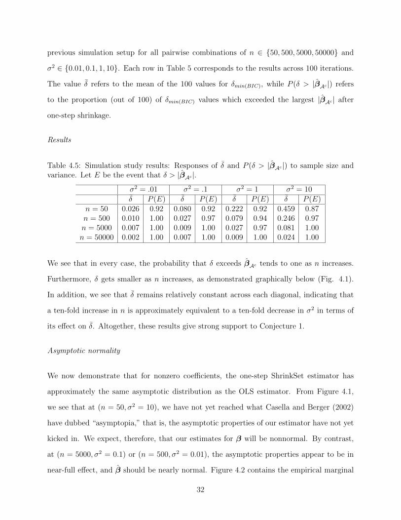
previous simulation setup for all pairwise combinations of n ∈ {50, 500, 5000, 50000} and
σ2 ∈ {0.01, 0.1, 1, 10}. Each row in Table 5 corresponds to the results across 100 iterations.
The value δ refers to the mean of the 100 values for δmin(BIC), while P (δ > |βAc|) refers
to the proportion (out of 100) of δmin(BIC) values which exceeded the largest |βAc | after
one-step shrinkage.
Results
Table 4.5: Simulation study results: Responses of δ and P (δ > |βAc|) to sample size andvariance. Let E be the event that δ > |βAc |.
σ2 = .01 σ2 = .1 σ2 = 1 σ2 = 10δ P (E) δ P (E) δ P (E) δ P (E)
n = 50 0.026 0.92 0.080 0.92 0.222 0.92 0.459 0.87n = 500 0.010 1.00 0.027 0.97 0.079 0.94 0.246 0.97n = 5000 0.007 1.00 0.009 1.00 0.027 0.97 0.081 1.00n = 50000 0.002 1.00 0.007 1.00 0.009 1.00 0.024 1.00
We see that in every case, the probability that δ exceeds βAc tends to one as n increases.
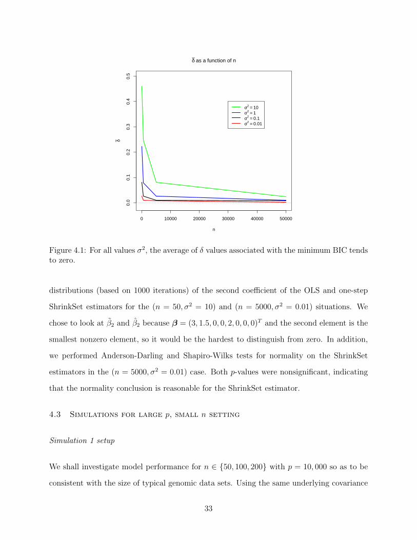
Furthermore, δ gets smaller as n increases, as demonstrated graphically below (Fig. 4.1).
In addition, we see that δ remains relatively constant across each diagonal, indicating that
a ten-fold increase in n is approximately equivalent to a ten-fold decrease in σ2 in terms of
its effect on δ. Altogether, these results give strong support to Conjecture 1.
Asymptotic normality
We now demonstrate that for nonzero coefficients, the one-step ShrinkSet estimator has
approximately the same asymptotic distribution as the OLS estimator. From Figure 4.1,
we see that at (n = 50, σ2 = 10), we have not yet reached what Casella and Berger (2002)
have dubbed “asymptopia,” that is, the asymptotic properties of our estimator have not yet
kicked in. We expect, therefore, that our estimates for β will be nonnormal. By contrast,
at (n = 5000, σ2 = 0.1) or (n = 500, σ2 = 0.01), the asymptotic properties appear to be in
near-full effect, and β should be nearly normal. Figure 4.2 contains the empirical marginal
32
Page 42
0 10000 20000 30000 40000 50000
0.0
0.1
0.2
0.3
0.4
0.5
δ as a function of n
n
δ
σ2 = 10σ2 = 1σ2 = 0.1σ2 = 0.01
Figure 4.1: For all values σ2, the average of δ values associated with the minimum BIC tendsto zero.
distributions (based on 1000 iterations) of the second coefficient of the OLS and one-step
ShrinkSet estimators for the (n = 50, σ2 = 10) and (n = 5000, σ2 = 0.01) situations. We
chose to look at β2 and β2 because β = (3, 1.5, 0, 0, 2, 0, 0, 0)T and the second element is the
smallest nonzero element, so it would be the hardest to distinguish from zero. In addition,
we performed Anderson-Darling and Shapiro-Wilks tests for normality on the ShrinkSet
estimators in the (n = 5000, σ2 = 0.01) case. Both p-values were nonsignificant, indicating
that the normality conclusion is reasonable for the ShrinkSet estimator.
4.3 Simulations for large p, small n setting
Simulation 1 setup
We shall investigate model performance for n ∈ {50, 100, 200} with p = 10, 000 so as to be
consistent with the size of typical genomic data sets. Using the same underlying covariance
33
Page 43
−1 0 1 2 3 4
0.0
0.1
0.2
0.3
0.4
0.5
0.6
Asymptotic normality has not yet been reached
N = 1000 Bandwidth = 0.1415
Den
sity
β2(ShrinkSet)β2(OLS)
1.494 1.496 1.498 1.500 1.502 1.504 1.506
050
100
150
200
Approximate asymptotic normality has been reached
N = 1000 Bandwidth = 0.0003795
Den
sity
β2(ShrinkSet)β2(OLS)
Figure 4.2: As expected, for sufficiently high n, the distribution of the ShrinkSet estimatoris similar to that of the OLS estimator (left panel: n = 50, σ2 = 10; right panel: n = 5000,σ2 = 0.01.)
structure as in the previous simulations, we define
β = (3, 1.5, 0, 0, 2, 0, 2.5, 2, 0, 0, 0, . . . , 0, 0, 0, 3, 4)T ∈ R10000.
(Note that the true model contains 7 nonzero coefficients.) We use σ2 = 1 and generate y
and X with appropriate dimensions. All simulations are the result of 100 iterations.
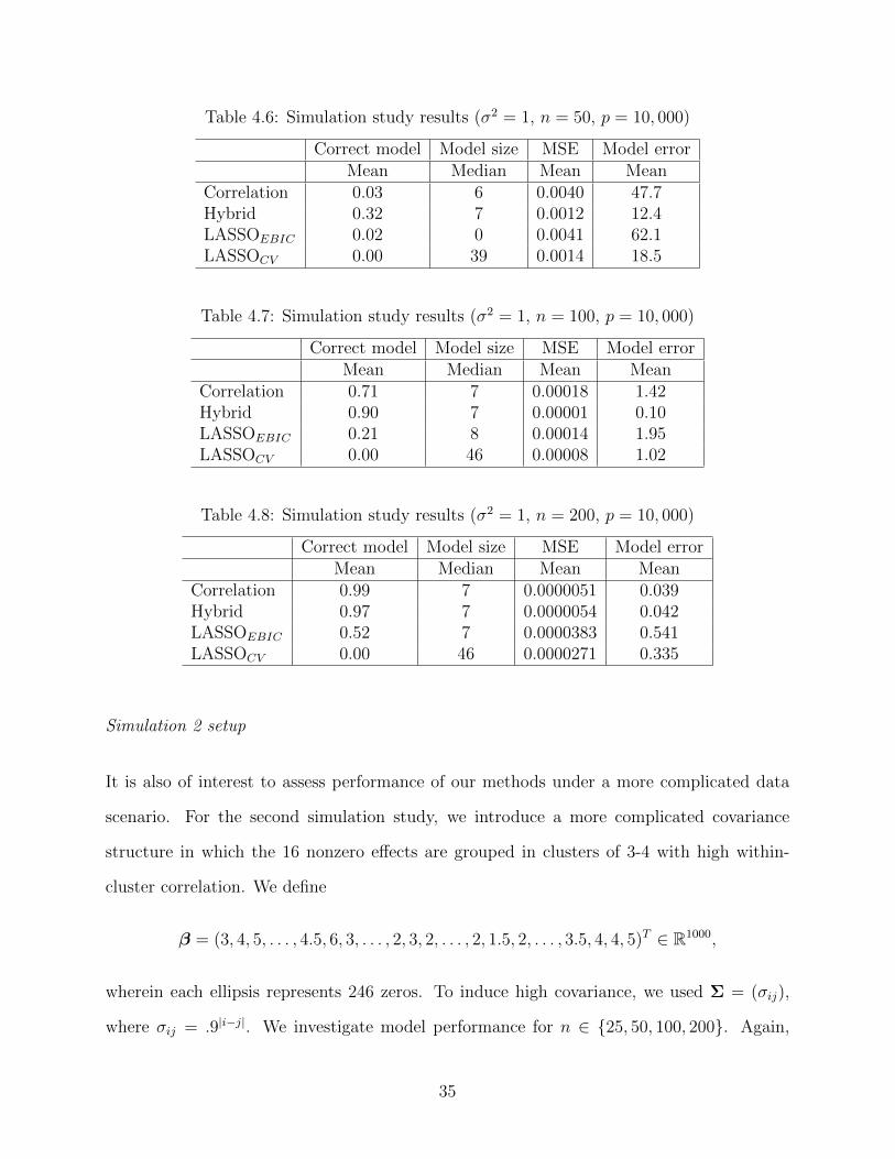
Results for Simulation 1
Our results indicate that the hybrid method outperforms LASSO for all sample sizes, and
that the correlation method outperforms LASSO in relatively high-n settings. More specifi-
cally, for all n studied, the hybrid method outperforms both LASSOs in every category. And
by n = 100, the correlation method is clearly better than both LASSO implementations.
For n = 200, only the correlation method outperforms the hybrid method, but the difference
is marginal. Overall, the hybrid method is probably best, because it is vastly superior to
LASSO in all settings, and only slightly worse than the correlation method in the high-n
setting but clearly better everywhere else.
34
Page 44
Table 4.6: Simulation study results (σ2 = 1, n = 50, p = 10, 000)
Correct model Model size MSE Model errorMean Median Mean Mean
Correlation 0.03 6 0.0040 47.7Hybrid 0.32 7 0.0012 12.4LASSOEBIC 0.02 0 0.0041 62.1LASSOCV 0.00 39 0.0014 18.5
Table 4.7: Simulation study results (σ2 = 1, n = 100, p = 10, 000)
Correct model Model size MSE Model errorMean Median Mean Mean
Correlation 0.71 7 0.00018 1.42Hybrid 0.90 7 0.00001 0.10LASSOEBIC 0.21 8 0.00014 1.95LASSOCV 0.00 46 0.00008 1.02
Table 4.8: Simulation study results (σ2 = 1, n = 200, p = 10, 000)
Correct model Model size MSE Model errorMean Median Mean Mean
Correlation 0.99 7 0.0000051 0.039Hybrid 0.97 7 0.0000054 0.042LASSOEBIC 0.52 7 0.0000383 0.541LASSOCV 0.00 46 0.0000271 0.335
Simulation 2 setup
It is also of interest to assess performance of our methods under a more complicated data
scenario. For the second simulation study, we introduce a more complicated covariance
structure in which the 16 nonzero effects are grouped in clusters of 3-4 with high within-
cluster correlation. We define
β = (3, 4, 5, . . . , 4.5, 6, 3, . . . , 2, 3, 2, . . . , 2, 1.5, 2, . . . , 3.5, 4, 4, 5)T ∈ R1000,
wherein each ellipsis represents 246 zeros. To induce high covariance, we used Σ = (σij),
where σij = .9|i−j|. We investigate model performance for n ∈ {25, 50, 100, 200}. Again,
35
Page 45
we use σ2 = 1 and generate y and X with appropriate dimensions. All simulations are the
result of 100 iterations.
Results for Simulation 2
These results indicate that the hybrid method outperforms all others for all but the n =
25 scenario, where no method does well. The hybrid method is exceptionally adept at
uncovering the correct sparse model. The correlation method has poor MSE and model error
at all levels of n included, but by n = 200, it outperforms both LASSOs in terms of selecting
the true model. Both implementations of LASSO always achieve low MSE, but in general
the hybrid method’s MSE is still lower. When compared to each other, LASSOCV tends to
have lower model error and LASSOEBIC tends select the correct model more frequently. For
the most difficult data scenario (n = 25), no method could uncover the true model, and all
suffered from severe over- or under-fitting.
Table 4.9: Simulation study results (σ2 = 1, n = 25, p = 1, 000)
Correct model Model size MSE Model errorMean Median Mean Mean
Correlation 0.00 2 0.42 494Hybrid 0.00 8 0.31 260LASSOEBIC 0.00 0 0.21 576LASSOCV 0.00 21 0.22 265
Table 4.10: Simulation study results (σ2 = 1, n = 50, p = 1, 000)
Correct model Model size MSE Model errorMean Median Mean Mean
Correlation 0.00 4 0.339 247.1Hybrid 0.17 15 0.037 12.1LASSOEBIC 0.00 17 0.095 182.5LASSOCV 0.00 36 0.032 12.8
36
Page 46
Table 4.11: Simulation study results (σ2 = 1, n = 100, p = 1, 000)
Correct model Model size MSE Model errorMean Median Mean Mean
Correlation 0.02 11 0.168 59.87Hybrid 0.89 16 0.002 0.23LASSOEBIC 0.02 21 0.004 1.61LASSOCV 0.00 36 0.003 0.83
Table 4.12: Simulation study results (σ2 = 1, n = 200, p = 1, 000)
Correct model Model size MSE Model errorMean Median Mean Mean
Correlation 0.35 16 0.0170 3.725Hybrid 1.00 16 0.0006 0.089LASSOEBIC 0.03 19 0.0014 0.574LASSOCV 0.00 30 0.0011 0.326
37
Page 48
chapter 5
DATA ANALYSIS
Analysis of HIV data set
Rhee, Taylor, Wadhera, Ben-Hur, Brutlag, and Shafer (2006) describe a publicly available
data set on HIV-1 drug resistance and codon mutation. The data consist of mutation
information for some 100 protease codons and a continuous response IC50, a measure of
HIV-1 drug resistance. We were interested in learning which codon mutations were related
to resistance to the drug Amprenavir, a protease inhibitor. This data set was also analyzed
by Dicker (2010), and we follow their example of removing codons with fewer than three
observed mutations and taking the log-transform of IC50. We present the results of our
method in connection with those of SELO, OLS (as used in the simulation setting), and
several other variable selection methods in terms of model size and R2 as a percentage of
the R2 value for complete OLS. One additional method presented is ShrinkSet2, which was
was obtained by removing the nonsignificant terms from the ShrinkSet estimator.
Model size R2/R2complete
OLS (α = .10) 30 0.985OLS (α = .05) 22 0.959OLS (α = .01) 17 0.949ShrinkSet 28 0.979ShrinkSet2 22 0.972SELO 16 0.958LASSO 32 0.959Adaptive LASSO 20 0.956SCAD 33 0.972
Table 5.1: Results of various variable selection procedures on HIV data set from Rhee et al.;ShrinkSet2 was obtained by removing the nonsignificant terms from the model in Table 5.2.
39
Page 49
Table 5.2: Codons selected by ShrinkSet method
Codon Point estimate Std. error Approx. p-valueP10 0.6605 0.0786 0.0000P11 0.4192 0.2258 0.0636P22 0.2738 0.4053 0.4990P24 0.3252 0.1471 0.0270P30 0.8879 0.1384 0.0000P32 0.9217 0.1786 0.0000P33 0.6724 0.0995 0.0000P34 0.4874 0.2220 0.0281P37 -0.2800 0.0644 0.0000P38 -0.3012 0.4083 0.4603P45 -0.3657 0.1705 0.0314P46 0.4853 0.0743 0.0000P47 1.0053 0.2222 0.0000P48 0.5978 0.1605 0.0002P50 0.5147 0.1546 0.0009P54 0.5387 0.0860 0.0000P64 -0.3951 0.0745 0.0000P65 -0.6255 0.2787 0.0250P66 -0.2858 0.1691 0.0908P67 0.2835 0.1954 0.1460P71 -0.3067 0.0765 0.0001P76 1.2616 0.1596 0.0000P83 -0.8397 0.4863 0.0840P84 0.8928 0.0893 0.0000P88 -1.3109 0.1151 0.0000P89 0.3378 0.1300 0.0094P90 0.6779 0.0790 0.0000P93 -0.3147 0.0622 0.0000
The ShrinkSet procedure explained more variation in y than all but OLS (α = .10),
yet it used fewer terms than OLS (α = .10), LASSO, and SCAD. The reasonable but slightly
ad hoc approach ShrinkSet2 was arguably the best of all, explaining the same amount of
variation as SCAD, but with 11 fewer terms. The following summary table (5.2) gives the
28 codons selected by the ShrinkSet method. Interestingly, 16 of the 17 most significant
p-values correspond to the 16 codons selected by SELO. The notable exception is codon 37,
which SELO did not select. Importantly, ShrinkSet selected mutations at codons 10, 32, 46,
40
Page 50
47, 50, 54, 76, 84, and 90, and these are known to be associated with Amprenavir resistance
(Johnson, Brun-Vezinet, Clotet, Gunthard, Kuritzkes, Pillay, Schapiro, and Richman 2010).
Analysis of salary data set
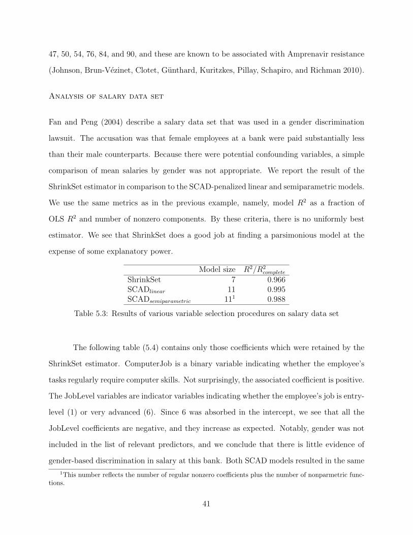
Fan and Peng (2004) describe a salary data set that was used in a gender discrimination
lawsuit. The accusation was that female employees at a bank were paid substantially less
than their male counterparts. Because there were potential confounding variables, a simple
comparison of mean salaries by gender was not appropriate. We report the result of the
ShrinkSet estimator in comparison to the SCAD-penalized linear and semiparametric models.
We use the same metrics as in the previous example, namely, model R2 as a fraction of
OLS R2 and number of nonzero components. By these criteria, there is no uniformly best
estimator. We see that ShrinkSet does a good job at finding a parsimonious model at the
expense of some explanatory power.
Model size R2/R2complete
ShrinkSet 7 0.966SCADlinear 11 0.995SCADsemiparametric 111 0.988
Table 5.3: Results of various variable selection procedures on salary data set
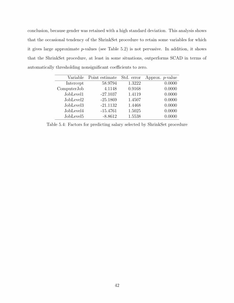
The following table (5.4) contains only those coefficients which were retained by the
ShrinkSet estimator. ComputerJob is a binary variable indicating whether the employee’s
tasks regularly require computer skills. Not surprisingly, the associated coefficient is positive.
The JobLevel variables are indicator variables indicating whether the employee’s job is entry-
level (1) or very advanced (6). Since 6 was absorbed in the intercept, we see that all the
JobLevel coefficients are negative, and they increase as expected. Notably, gender was not
included in the list of relevant predictors, and we conclude that there is little evidence of
gender-based discrimination in salary at this bank. Both SCAD models resulted in the same
1This number reflects the number of regular nonzero coefficients plus the number of nonparmetric func-tions.
41
Page 51
conclusion, because gender was retained with a high standard deviation. This analysis shows
that the occasional tendency of the ShrinkSet procedure to retain some variables for which
it gives large approximate p-values (see Table 5.2) is not pervasive. In addition, it shows
that the ShrinkSet procedure, at least in some situations, outperforms SCAD in terms of
automatically thresholding nonsignificant coefficients to zero.
Variable Point estimate Std. error Approx. p-valueIntercept 58.9794 1.3222 0.0000
ComputerJob 4.1148 0.9168 0.0000JobLevel1 -27.1037 1.4119 0.0000JobLevel2 -25.1869 1.4507 0.0000JobLevel3 -21.1132 1.4468 0.0000JobLevel4 -15.4761 1.5025 0.0000JobLevel5 -8.8612 1.5538 0.0000
Table 5.4: Factors for predicting salary selected by ShrinkSet procedure
42
Page 52
chapter 6
CONCLUSIONS AND FURTHER RESEARCH
We have proposed a novel variable selection method based upon an obscure penalty function
that mimics the L0 penalty. Unlike other variable selection penalties, the ShrinkSet penalty
is everywhere-differentiable and everywhere-continuous, allowing for an efficient iterative
ridge algorithm capable of finding the approximate maximizer of the associated penalized
likelihood in very few iterations. Because the penalty is not singular at the origin, the
associated maximizer does not produce sparse solutions, despite having shrunk irrelevant
coefficients very close to zero. We therefore employ a zero-thresholding step based upon
a shrinkage parameter δ in order to obtain the ShrinkSet estimator. Unlike some existing
methods, the ShrinkSet procedure explicitly estimates this thresholding parameter in its
normal implementation, and requires no additional computation to do so.
We have given strong evidence for the asymptotic oracle properties of our estimator
and have compared its finite-sample performance to that of several leading methods in var-
ious simulation and data analysis settings. In all scenarios studied, the ShrinkSet estimator
either outperformed or was on par with other variable selection procedures. In addition,
we maintain that the smooth nature of the penalty allows for optimization that is both
computationally efficient and pedagogically appealing.
While this project has set forth some of the most important properties of the ShrinkSet
estimator, there is still much to be learned. As mentioned in the text, further research could
focus on establishing the oracle properties of the robust and generalized linear estimators.
In addition, there may be other effective implementations of the ShrinkSet penalty in the
p� n setting. Finally, formal proofs of the conjectures set forth in this project would help to
solidify the ShrinkSet procedure’s position in the class of effective variable selection methods.
43
Page 53
The fact that there are still unanswered questions should not dissuade readers from using
the ShrinkSet procedure, however. It has been almost two decades since the LASSO was
first introduced, but statisticians today continue to make great discoveries while studying
its properties. We suspect that further investigations into the ShrinkSet procedure would
likewise benefit and enrich the field.
44
Page 54
BIBLIOGRAPHY
Akaike, H. (1974), “A new look at the statistical model identification,” IEEE Transactions
on Automatic Control, 19, 716–723.
Antoniadis, A., and Fan, J. (2001), “Regularization of Wavelet Approximations,” Journal
of the American Statistical Association, 96, 939–955.
Antoniadis, A., Gijbels, I., and Nikolova, M. (2009), “Penalized likelihood regression for gen-
eralized linear models with non-quadratic penalties,” Annals of the Institute of Statistical
Mathematics, Online First.
Breiman, L. (1995), “Better Subset Regression Using the Nonnegative Garrote,” Techno-
metrics, 37, 373–384.
—— (1996), “Heuristics of instability and stabilization in model selection,” The Annals of
Statistics, 24, 2350–2383.
—— (2001), “Random Forests,” Machine Learning, 45, 5–32.
Candes, E., and Tao, T. (2007), “The Dantzig selector: Statistical estimation when p is
much larger than n,” The Annals of Statistics, 35, 2313–2351.
Corepetti, T., Heitz, D., Arroyo, G., Memin, E., and Santa-Cruz, A. (2006), “Fluid ex-
perimental flow estimation based on an optical-flow scheme,” Experiments in Fluids, 40,
80–97.
Dicker, L. (2010), “Regularized regression methods for variable selection and estimation
(PhD dissertation, Harvard University),” Dissertations and Theses: Full Text [ProQuest
online database], Publication number: AAT 3414668.
45
Page 55
Doksum, K., Tang, S., and Tsui, K.-W. (2008), “Nonparametric Variable Selection: The
EARTH Algorithm,” Journal of the American Statistical Association, 103, 1609–1620.
Efron, B., Hastie, T., Johnstone, I., and Tibshirani, R. (2004), “Least Angle Regression,”
The Annals of Statistics, 32, 407–499.
Fan, J., and Li, R. (2001), “Variable Selection via Nonconcave Penalized Likelihood and Its
Oracle Properties,” Journal of the American Statistical Association, 96, 1348–1360.
Fan, J., and Lv, J. (2008), “Sure independence screening for ultrahigh dimensional feature
space,” Journal of the Royal Statistical Society. Series B (Statistical Methodology), 70,
859–911.
Fan, J., and Peng, H. (2004), “Nonconcave Penalized Likelihood with a Diverging Number
of Parameters,” The Annals of Statistics, 32, 928–961.
Fessler, J. A. (1996), “Mean and Variance of Implicitly Defined Biased Estimators (Such as
Penalized Maximum Likelihood) : Applications to Tomography,” IEEE Transactions on
Image Processing, 5, 493–506.
Frank, I. E., and Friedman, J. H. (1993), “A Statistical View of Some Chemometrics Re-
gression Tools,” Technometrics, 35, 109–135.
Friedman, J. H., Hastie, T., and Tibshirani, R. (2010), “Regularization Paths for Generalized
Linear Models via Coordinate Descent,” Journal of Statistical Software, 33, 1–22.
Fu, W. J. (1998), “Penalized Regressions: The Bridge versus the Lasso,” Journal of Com-
putational and Graphical Statistics, 7, 397–416.
Hastie, T., Tibshirani, R., and Friedman, J. (2009), The Elements of Statistical Learning
(2nd ed.), New York: Springer.
Hoerl, A. E., and Kennard, R. W. (1970), “Ridge Regression: Biased Estimation for
Nonorthogonal Problems,” Technometrics, 12, 55–67.
46
Page 56
Huber, P. (1964), “Robust Estimation of a Location Parameter,” The Annals of Statistics,
53, 73–101.
Johnson, V. A., Brun-Vezinet, F., Clotet, B., Gunthard, H., Kuritzkes, D., Pillay, D.,
Schapiro, J., and Richman, D. (2010), “Update of the Drug Resistance Mutations in
HIV-1: December 2010,” Topics in HIV Medicine, 18, 156–163.
Lian, H. (2010), “Flexible Shrinkage Estimation in High-Dimensional Varying Coefficient
Models,” arXiv.org, arXiv:1008.2271v1.
Mallows, C. L. (1973), “Some Comments on Cp,” Technometrics, 15, 661–675.
Mitchell, T. J., and Beauchamp, J. J. (1988), “Bayesian variable selection in linear regres-
sion,” Journal of the American Statistical Association, 83, 1023–1036.
Nikolova, M. (2005), “Analysis of the Recovery of Edges in Images and Signals by Minimizing
Non-convex Regularized Least-squares,” Multiscale Modeling and Simulation, 4, 960–991.
Rhee, S.-Y., Taylor, J., Wadhera, G., Ben-Hur, A., Brutlag, D. L., and Shafer, R. W.
(2006), “Genotypic Predictors of Human Immunodeficiency Virus Type 1 Drug Resis-
tance,” Proceedings of the National Academy of Sciences of the United States of America,
46, 17355–17360.
Schwarz, G. (1978), “Estimating the dimension of a model,” The Annals of Statistics, 6,
461–464.
Tibshirani, R. (1996), “Regression Shrinkage and Selection via the Lasso,” Journal of the
Royal Statistical Society. Series B (Methodological), 58, 267–288.
Wang, H., Li, R., and Tsai, C.-L. (2007), “Tuning Parameter Selectors for the Smoothly
Clipped Absolute Deviaation Method,” Biometrika, 94, 553–568.
Wikel, J. H., and Dow, E. R. (1993), “The use of neural networks for variable selection in
QSAR,” Bioorganic and Medicinal Chemistry Letters, 3, 645–651.
47
Page 57
Zou, H. (2006), “The Adaptive Lasso and Its Oracle Properties,” Journal of the American
Statistical Association, 101, 1418–1429.
Zou, H., and Hastie, T. (2005), “Regularization and variable selection via the elastic net,”
Journal of the Royal Statistical Society. Series B (Methodological), 67, 301–320.
Zou, H., Hastie, T., and Tibshirani, R. (2007), “On the “Degrees of Freedom” of the LASSO,”
The Annals of Statistics, 35, 2173–2192.
Zou, H., and Li, R. (2008), “One-step sparse estiamtes in nonconcave penalized likelihood
models,” The Annals of Statistics, 36, 1509–1533.
48