The Annals of Statistics 2002, Vol. 30, No. 1, 74–99 VARIABLE SELECTION FOR COX’S PROPORTIONAL HAZARDS MODEL AND FRAILTY MODEL BY J IANQING FAN 1 AND RUNZE LI 2 Chinese University of Hong Kong and Pennsylvania State University A class of variable selection procedures for parametric models via nonconcave penalized likelihood was proposed in Fan and Li (2001a). It has been shown there that the resulting procedures perform as well as if the subset of significant variables were known in advance. Such a property is called an oracle property. The proposed procedures were illustrated in the context of linear regression, robust linear regression and generalized linear models. In this paper, the nonconcave penalized likelihood approach is extended further to the Cox proportional hazards model and the Cox proportional hazards frailty model, two commonly used semi-parametric models in survival analysis. As a result, new variable selection procedures for these two commonly-used models are proposed. It is demonstrated how the rates of convergence depend on the regularization parameter in the penalty function. Further, with a proper choice of the regularization parameter and the penalty function, the proposed estimators possess an oracle property. Standard error formulae are derived and their accuracies are empirically tested. Simulation studies show that the proposed procedures are more stable in prediction and more effective in computation than the best subset variable selection, and they reduce model complexity as effectively as the best subset variable selection. Compared with the LASSO, which is the penalized likelihood method with the L 1 -penalty, proposed by Tibshirani, the newly proposed approaches have better theoretic properties and finite sample performance. 1. Introduction. An objective of survival analysis is to identify the risk factors and their risk contributions. Often, many covariates are collected and to reduce possible modeling bias, a large parametric model is built. An important and challenging task is to efficiently select a subset of significant variables upon which the hazard function depends. There are many variable selection techniques in linear regression models. Some of them have been extended to the context of censored survival data analysis, such as the best subset variable selection and stepwise deletion. Bayesian variable selection methods for censored survival data were proposed by Faraggi and Simon (1998), based on an idea of Lindley (1968). Received November 2000; revised August 2001. 1 Supported in part by NIH Grant IR01CA92571-01, NSF Grant DMS-01-96041 and RGC Grant CUHK4262/01P of HKSAR. 2 Supported by NSF Grant DMS-01-02505. AMS 2000 subject classifications. 62F12, 62N02. Key words and phrases. Cox’s regression model, frailty model, LASSO, penalized likelihood, partial likelihood, profile likelihood. 74
Transcript
The Annals of Statistics2002, Vol. 30, No. 1, 74–99
VARIABLE SELECTION FOR COX’S PROPORTIONAL HAZARDSMODEL AND FRAILTY MODEL
BY JIANQING FAN1 AND RUNZE LI2
Chinese University of Hong Kong and Pennsylvania State University
A class of variable selection procedures for parametric models vianonconcave penalized likelihood was proposed in Fan and Li (2001a). Ithas been shown there that the resulting procedures perform as well as ifthe subset of significant variables were known in advance. Such a propertyis called an oracle property. The proposed procedures were illustrated inthe context of linear regression, robust linear regression and generalizedlinear models. In this paper, the nonconcave penalized likelihood approachis extended further to the Cox proportional hazards model and the Coxproportional hazards frailty model, two commonly used semi-parametricmodels in survival analysis. As a result, new variable selection procedures forthese two commonly-used models are proposed. It is demonstrated how therates of convergence depend on the regularization parameter in the penaltyfunction. Further, with a proper choice of the regularization parameter andthe penalty function, the proposed estimators possess an oracle property.Standard error formulae are derived and their accuracies are empiricallytested. Simulation studies show that the proposed procedures are morestable in prediction and more effective in computation than the best subsetvariable selection, and they reduce model complexity as effectively as thebest subset variable selection. Compared with the LASSO, which is thepenalized likelihood method with the L1-penalty, proposed by Tibshirani, thenewly proposed approaches have better theoretic properties and finite sampleperformance.
1. Introduction. An objective of survival analysis is to identify the riskfactors and their risk contributions. Often, many covariates are collected and toreduce possible modeling bias, a large parametric model is built. An importantand challenging task is to efficiently select a subset of significant variables uponwhich the hazard function depends. There are many variable selection techniquesin linear regression models. Some of them have been extended to the context ofcensored survival data analysis, such as the best subset variable selection andstepwise deletion. Bayesian variable selection methods for censored survival datawere proposed by Faraggi and Simon (1998), based on an idea of Lindley (1968).
Received November 2000; revised August 2001.1Supported in part by NIH Grant IR01CA92571-01, NSF Grant DMS-01-96041 and RGC Grant
CUHK4262/01P of HKSAR.2Supported by NSF Grant DMS-01-02505.AMS 2000 subject classifications. 62F12, 62N02.Key words and phrases. Cox’s regression model, frailty model, LASSO, penalized likelihood,
partial likelihood, profile likelihood.
74
VARIABLE SELECTION FOR COX’S MODEL 75
Despite their popularity, the sampling properties of the aforementioned selectionmethods are largely unknown and confidence intervals derived from the selectedvariables may not have right coverage probabilities.
Fan and Li (2001a) proposed a family of new variable selection methods basedon a nonconcave penalized likelihood approach. The proposed methods are differ-ent from traditional approaches of variable selection in that they delete insignifi-cant variables by estimating their coefficients as 0. Thus their approaches simulta-neously select significant variables and estimate regression coefficients. LASSO,proposed by Tibshirani (1996, 1997), is a member of this family with the L1-penalty. See also Knight and Fu (2000) for asymptotic properties of lasso-typeestimators. The penalized likelihood approach was applied to linear regression, ro-bust linear regression and generalized linear models. From their simulations, Fanand Li (2001a) showed the proposed penalized likelihood estimator with smoothlyclipped absolute deviation penalty (defined in Section 2, the name of SCAD refersto the procedures related to this penalty function) outperforms the best subsetvariable selection in terms of computational cost and stability, in the terminol-ogy of Breiman (1996). The SCAD improves the LASSO via reducing estima-tion bias. Furthermore, they showed that the SCAD possesses an oracle propertywith a proper choice of regularization parameter, in the terminology of Donohoand Johnstone (1994). Namely, the true regression coefficients that are zero areautomatically estimated as zero, and the remaining coefficients are estimated aswell as if the correct submodel were known in advance. Hence, the SCAD andits siblings are an ideal procedure for variable selection, at least from the theo-retical point of view. This encourages us to investigate their properties in Cox’sproportional hazards model and frailty model, two popularly used semiparametricmodels.
It will be shown that the proposed penalized likelihood for the Cox regressionmodel is equivalent to a penalized partial likelihood. This new approach canselect significant variables and estimate regression coefficients simultaneously.This allows one to construct a confidence interval for coefficients easily. Ratesof convergence of the penalized partial likelihood estimators are established.Further, with proper choice of regularization parameters, we will show that theSCAD performs as well as an oracle estimator. The significance of this is that theproposed procedure outperforms the maximum partial likelihood estimator whentrue coefficients have zero components and performs as well as if one knew thetrue submodel. This result is closely related to the super-efficiency phenomenon,given by the Hodges example [Lehmann (1983), page 405]. In addition, a modifiedNewton–Raphson algorithm is developed for maximizing the penalized partiallikelihood function, and a standard error formula for estimated coefficients ofnonzero components is derived by using a sandwich formula. The standard errorformula is empirically tested for the Cox regression model. It performs verywell with moderate sample sizes. The proposed method compares favorably with
76 J. FAN AND R. LI
the best subset variable selection, in terms of performance, model stability andcomputation.
Unlike the Cox regression model, there are some challenges in parameter es-timation in the Cox frailty model even without the task of model selection. Infact, with the “least informative” nonparametric modeling for the baseline cumu-lative hazard function, the corresponding profile likelihood of the frailty modeldoes not have a closed form. This poses some challenges to find estimates forparameters of interest. A new iterative procedure for this semi-parametric frailtymodel is proposed in order to find the profile maximum likelihood estimator. Itprovides a useful alternative to the EM algorithm for the frailty model, even with-out the task of variable selection. Standard error formulas are derived and empir-ically tested. Further, the penalized likelihood approach is extended to the semi-parametric frailty model via penalizing the profile likelihood function. Due to itssimultaneous selection of significant variables and estimation of regression coef-ficients, our approach allows one to construct confidence intervals for unknowncoefficients via a sandwich formula. The corresponding sandwich formula is anestimator for the covariance matrix of the estimated coefficients. The Newton–Raphson algorithm with some modifications is used to find the solution of penal-ized profile likelihood score equations. It performs very well for moderate samplesize. Again, in this model, SCAD outperforms the best subset variable selectionand LASSO.
The paper is organized as follows. Motivations of variable selection via non-concave penalized likelihood are briefly given in Section 2. A new variable selec-tion procedure for the Cox model and Cox frailty model is proposed in Section 3,in which the consistency and an oracle property of the proposed procedures areestablished. A modification of the Newton–Raphson algorithm and standard er-ror formulae for estimated coefficients are also presented in Section 3. Section 4gives numerical comparisons among the newly proposed approach, the LASSOand the best subset variable selection. Proofs of main results are given in Sec-tion 5.
2. Variable selection via nonconcave penalized likelihood. Assume thatthe collected data (xi, Yi) are independent samples. Conditioning on xi , Yi hasa density fi(yi; xT
i β). Denote by �i = log fi , the conditional log-likelihood ofYi given xi . As discussed in Fan and Li (2001a), a general form of penalizedlikelihood is
n∑i=1
�i
(yi; xT
i β)− n
d∑j=1
pλ(|βj |),(2.1)
where d is the dimension of β , pλ(·) is a penalty function and λ is a tuningparameter (more generally, it is allowed to use λj ). Some conditions on pλ(| · |)are needed in order for the approach to be an effective variable selection procedure
VARIABLE SELECTION FOR COX’S MODEL 77
[Antoniadis and Fan (2001)]. In particular, pλ(| · |) should be irregular at theorigin, that is, p′
λ(0+) > 0. Denote by β0 the true value of β , and let β0 =(β10, . . . , βd0)T = (βT
10,βT20)T . Without loss of generality, it is assumed that
β20 = 0, and all components of β10 are not equal to 0. Under some regularity
conditions, Fan and Li (2001a) showed their SCAD estimator β = (βT
1 , βT
2 )T
possesses the following oracle property. With probability tending to 1, for certainchoice of pλn(·), we have β2 = 0 and
√n(β1 − β10
)→ N{0, I−1
1 (β10, 0)},
where I1(β10, 0) is the Fisher information matrix for β1 knowing β2 = 0.For linear regression models, when the columns of the design matrix X are
orthonormal, it is easy to show that the best subset selection and stepwise deletionare equivalent to the penalized least squares estimator with the hard thresholdingpenalty, defined by
pλ(|θ |) = λ2 − (|θ | − λ)2I (|θ | < λ).
This penalty function was proposed by Fan (1997) and improved by Antoniadis(1997). The name HARD refers to the procedure related to the hard thresholdingpenalty. The hard thresholding penalty does not overpenalize the large value of |θ |.Note that when a design matrix is not orthonormal, the penalized least-squares, thestepwise deletion and the best subset methods may not be equivalent. Other penaltyfunctions have been used in the literature. The L2-penalty pλ(|θ |) = λ|θ |2 resultsin a ridge regression. The L1-penalty pλ(|θ |) = λ|θ | yields LASSO, proposed byDonoho and Johnstone (1994) in the wavelet setting and extended by Tibshirani(1996, 1997) to general likelihood settings.
A good penalty function should result in an estimator with the followingthree properties: unbiasedness for a large true coefficient to avoid excessiveestimation bias, sparsity (estimating a small coefficient as zero) to reduce modelcomplexity, and continuity to avoid unnecessary variation in model prediction.Necessary conditions for unbiasedness, sparsity and continuity have been derivedby Antoniadis and Fan (2001). However, all of the L1, L2 (indeed all of Lp-penalty) and the HARD penalties do not simultaneously satisfy these threemathematical conditions.
A simple penalty function that satisfies all the three mathematical requirementsis the smoothly clipped absolute deviation (SCAD) penalty, defined by
p′λ(θ) = I (θ ≤ λ) + (aλ − θ)+
(a − 1)λI (θ > λ) for some a > 2 and θ > 0.(2.2)
This function was proposed by Fan (1997) and involves two unknown parame-ters λ and a. In practice, one could search the best pair (λ, a) over two dimensionalgrids using some criteria, such as cross-validation and generalized cross-validation
78 J. FAN AND R. LI
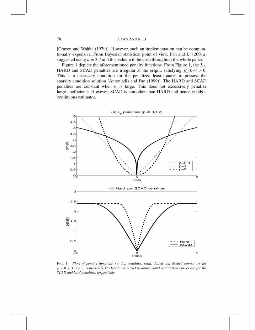
[Craven and Wahba (1979)]. However, such an implementation can be computa-tionally expensive. From Bayesian statistical point of view, Fan and Li (2001a)suggested using a = 3.7 and this value will be used throughout the whole paper.
Figure 1 depicts the aforementioned penalty functions. From Figure 1, the L1,HARD and SCAD penalties are irregular at the origin, satisfying p′
λ(0+) > 0.This is a necessary condition for the penalized least-squares to possess thesparsity condition solution [Antoniadis and Fan (1999)]. The HARD and SCADpenalties are constant when θ is large. This does not excessively penalizelarge coefficients. However, SCAD is smoother than HARD and hence yields acontinuous estimator.
FIG. 1. Plots of penalty functions. (a) Lp penalties, solid, dotted and dashed curves are forp = 0.3, 1 and 2, respectively. (b) Hard and SCAD penalties, solid and dashed curves are for theSCAD and hard penalties, respectively.
VARIABLE SELECTION FOR COX’S MODEL 79
3. Proportional hazards models. Let T, C and x be respectively the survivaltime, the censoring time and their associated covariates. Correspondingly, let Z =min{T, C} be the observed time and δ = I (T ≤ C) be the censoring indicator. It isassumed that T and C are conditionally independent given x and that the censoringmechanism is noninformative. When the observed data {(xi, Zi, δi) : i = 1, . . . , n}is an independently and identically distributed random sample from a certainpopulation (x, Z, δ), a complete likelihood of the data is given by
L =∏u
f (Zi |xi )∏c
F (Zi |xi) =∏u
h(Zi |xi)
n∏i=1
F (Zi |xi),(3.1)
where the subscripts c and u denote the product of the censored and uncensoreddata respectively, and f (t|x), F (t|x) and h(t|x) are the conditional densityfunction, the conditional survival function and the conditional hazard functionof T given x. Statistical inference in this paper will be based on the likelihoodfunction (3.1).
To present explicitly the likelihood function of Cox’s proportional hazards mod-el, more notation is needed. Let t0
times. Let (j) provide the label for the item falling at t0j so that the covariates
associated with the N failures are x(1), . . . , x(N). Let Rj denote the risk set rightbefore the time t0
j:
Rj = {i : Zi ≥ t0
j
}.
Consider proportional hazards models,
h(t|x) = h0(t) exp(xT β
),(3.2)
with the baseline hazard functions h0(t) and parameter β . The likelihood in (3.1)becomes
L =N∏
i=1
h0(Z(i)) exp(xT
(i)β) n∏
i=1
exp{−H0(Zi) exp
(xT
i β)}
,
where H0(·) is the cumulative baseline hazard function. If the baseline hazardfunction has a parametric form, h0(θ , ·) say, then the corresponding penalized log-likelihood function is
N∑i=1
[log{h0(θ, Z(i))} + xT
(i)β]
(3.3)
−n∑
i=1
{H0(θ , Zi) exp
(xT
i β)}− n
d∑j=1
pλ(|βj |).
Maximizing (3.3) with respect to (θ ,β) yields the maximum penalized likelihoodestimator.
80 J. FAN AND R. LI
3.1. Penalized partial likelihood. In the Cox proportional hazards model, thebaseline hazard function is unknown and has not been parameterized. FollowingBreslow’s idea, consider the “least informative” nonparametric modeling forH0(·), in which H0(t) has a possible jump hj at the observed failure time t0
j . More
precisely, let H0(t) =∑Nj=1 hj I (t0
j ≤ t). Then
H0(Zi) =N∑
j=1
hj I (i ∈ Rj ).(3.4)
Using (3.4), the logarithm of penalized likelihood function of (3.3) becomes
N∑j=1
{log(hj ) + xT
(j)β}
−n∑
i=1
{N∑
j=1
hjI (i ∈ Rj ) exp(xT
i β)}− n
d∑j=1
pλ(|βj |).(3.5)
Taking the derivative with respect to hj and setting it to be zero, we obtain that
hj ={ ∑
i∈Rj
exp(xTi β)
}−1
.(3.6)
Substituting hj into (3.5), we get the penalized partial likelihood
N∑j=1
[xT
(j)β − log
{∑i∈Rj
exp(xT
i β)}]− n
d∑j=1
pλ(|βj |),(3.7)
after dropping a constant term “−N”. When pλ(·) ≡ 0, (3.7) is the partiallikelihood function [Cox (1975)]. The penalized likelihood estimate of β is derivedby maximizing (3.7) with respect to β . With a proper choice of pλ, many of theestimated coefficients will be zero and hence their corresponding variables do notappear in the model. This achieves the objectives of variable selection.
3.2. Frailty model. It is assumed for the Cox proportional hazards modelthat the survival times of subjects are independent. This assumption might beviolated in some situations, in which the collected data are correlated. One popularapproach to model correlated survival times is to use a frailty model. A frailtycorresponds to a random block effect that acts multiplicatively on the hazard ratesof all subjects in a group. In this section, we only consider the Cox proportionalhazard frailty model, in which it is assumed that the hazard rate for the j th subjectin the ith subgroup is
hij (t|xij , ui) = h0(t)ui exp(xT
ijβ), i = 1, . . . , n, j = 1, . . . , Ji,(3.8)
VARIABLE SELECTION FOR COX’S MODEL 81
where the ui’s are associated with frailties, and they are a random sample fromsome population. It is frequently assumed that given the frailty ui , the data in theith group are independent. The most frequently used distribution for frailty is thegamma distribution due to its simplicity. Assume without loss of generality that themean of frailty is 1 so that all parameters involved are estimable. For the gammafrailty model, the density of u is
g(u) = ααuα−1 exp(−α u)
&(α).
From (3.1), the full likelihood of “pseudo-data" {(ui, Xij , Zij , δij ) : i = 1, . . . , n,j = 1 . . . , Ji} is
n∏i=1
Ji∏j=1
[{h(zij |xij , ui)}δij F (zij |xij , ui)] n∏
i=1
g(ui).
Integrating the full likelihood function with respect to u1, . . . , un, the likelihood ofthe observed data is given by
L(β, α, H) = exp
{βT
(n∑
i=1
Ji∑j=1
δij xij
)}(3.9)
×n∏
i=1
αα ∏Ji
j=1{h0(zij )}δij
&(α){∑Ji
j=1 H0(zij ) exp(xTijβ) + α}(Ai+α)
,
where Ai =∑Ji
j=1 δij . Therefore the logarithm of the penalized likelihood of theobserved data is
n∑i=1
{Ji∑
j=1
δij log h(zij ) −[
(Ai + α) log
{Ji∑
j=1
H0(zij ) exp(xT
ijβ)+ α
}]}(3.10)
+n∑
i=1
{βT
(Ji∑
j=1
δij xij
)+ α log α − log &(α)
}− n
d∑j=1
pλ(|βj |).
To eliminate the nuisance parameter h(·), we again employ the profile likelihoodmethod. Consider the “least informative" nonparametric modeling for H0(·):
H0(z) =N∑
l=1
λlI (zl ≤ z),(3.11)
where {z1, . . . , zN} are pooled observed failure times.Substituting (3.11) into (3.10), then differentiating it with respect to λl , l =
1, . . . , N , the root of the corresponding score function should satisfy the following
82 J. FAN AND R. LI
equations:
λ−1l =
n∑i=1
(Ai + α)∑Ji
j=1 I (zl ≤ zij ) exp(xTij β)∑N
k=1 λk
∑Ji
j=1 I (zk ≤ zij ) exp(xTij β) + α
(3.12)
for l = 1, . . . , N .The above solution does not admit a closed form, and neither does the profile
likelihood function. However, the maximum profile likelihood can be implementedas follows. With initial values for α,β and λl , update {λl} from (3.12) and obtainthe penalized profile likelihood of (3.10). With known H0(·) defined by (3.11),maximize the penalized likelihood (3.10) with respect to (α,β), and iteratebetween these two steps. When the Newton–Raphson algorithm is applied to thepenalized likelihood (3.10), it involves the first two order derivatives of the gammafunction, which may not exist for certain value of α. One approach to avoid thisdifficulty is the use of a grid of possible values for the frailty parameter α andfinding the maxima over this discrete grid, as suggested by Nielsen et al. (1992).Our simulation experience shows that the estimate of β is quite empirically robustto the chosen grid of possible values for α. This profile likelihood method appearsnew even without the task of variable selection. This provides a viable alternativeapproach to the EM algorithm frequently used in the frailty model.
A natural initial estimator for β is the maximum pseudo-partial likelihood es-timates of β ignoring possible dependency within each group. The correspondingh1, . . . , hN in (3.6) may serve as an initial estimator for λ1, . . . , λN . Hence given avalue of α and initial values of β and λ1, . . . , λN , update the values of λ1, . . . , λN
and α, β in turn until they converge or the penalized profile likelihood of (3.10)fails to change substantially. The proposed algorithm avoids optimizing a high-dimensional problem. It will give us an efficient estimate for β . The algorithmmay converge slowly or even not converge. In this situation, the idea of one-stepestimator [see Bickel (1975)] provides us an alternative approach. See Section 3.4for some other variations.
3.3. Oracle properties. We will use the theory of counting processes toestablish the oracle property of the proposed variable selection approach for theCox model under general settings. Following the notation in Andersen and Gill(1982), define Ni(t) = I {Ti ≤ t, Ti ≤ Ci} and Yi(t) = I {Ti ≥ t, Ci ≥ t}. In thissection, the covariate x is allowed to be time-dependent, denoted by x(t). Forsimplicity, we shall work on the finite time interval [0, τ ]. Assume without loss ofgenerality that τ = 1. One may extend the results to the interval [0,∞), followingthe proof for Theorem 4.2 of Anderson and Gill (1982). We need the followingconditions to establish the oracle property.
CONDITIONS. A.∫ 1
0 h0(t) dt < ∞.B. The processes x(t) and Y (t) are left-continuous with right hand limits, and
P {Y (t) = 1 ∀t ∈ [0, 1]} > 0.
VARIABLE SELECTION FOR COX’S MODEL 83
C. There exists a neighborhood B of β0 such that
E supt∈[0,1],β∈B
Y (t)x(t)T x(t) exp(βT x(t)
}< ∞.
D. Define
s(0)(β, t) = EY (t) exp{βT x(t)
},
s(1)(β, t) = EY (t)x(t) exp{βT x(t)
},
s(2)(β, t) = EY (t)x(t)x(t)T exp{βT x(t)
},
where s(0)(·, t), s(1)(·, t) and s(2)(·, t) are continuous in β ∈ B , uniformly int ∈ [0, 1]. s(0), s(1) and s(2) are bounded on B × [0, 1]; s(0) is bounded awayfrom zero on B × [0, 1]. The matrix
I (β0) =∫ 1
0v(β0, t)s(0)(β0, t)h0(t) dt
is finite positive definite, where
v(β, t) = s(2)
s(0)−(
s(1)
s(0)
)(s(1)
s(0)
)T
.
Conditions A–D guarantee the local asymptotic quadratic (LAQ) propertyfor the partial likelihood function, and hence the asymptotic normality of themaximum partial likelihood estimates. See Andersen and Gill (1982) and Murphyand van der Vaart (2000) for details.
In this section we will show that the proposed estimators perform as well asan oracle estimator. Let β0 = (β10, . . . , βd0)T = (βT
10,βT20)T . Without loss of
generality, assume that β20 = 0. Denote by s the number of the components ofβ1,
an = max{p′λn
(|βj0|) : βj0 �= 0} and
bn = max{|p′′λn
(|βj0|)| : βj0 �= 0}.(3.13)
It will be shown that there exists a penalized partial likelihood estimator thatconverges at rate OP (n−1/2 + an). Oracle properties for the penalized partiallikelihood estimator will be also established. In this section, we only state theoreticresults. Their proofs will be given in Section 5.
The following theorem shows how the rates of convergence for the penalizedpartial likelihood estimators depend on the regularization parameter. Let �(β) =∑N
j=1[xT(j)β − log{∑i∈Rj
exp(xTi β)}] denote the log-partial likelihood function
and let Q(β) = �(β) − n∑d
j=1 pλ(|βj |) be the penalized partial likelihoodfunction.
84 J. FAN AND R. LI
THEOREM 3.1. Assume that (x1, T1, C1), . . . , (xn, Tn, Cn) are independentand identically distributed according to the population (x, T , C), T and C areconditionally independent given x, and Conditions (A)–(D) hold. If bn → 0, thenthere exists a local maximizer β of Q(β) such that ‖β − β0‖ = OP (n−1/2 + an),where an is given by (3.13).
It is clear from Theorem 3.1 that by choosing a proper λn, there exists aroot-n consistent penalized partial likelihood estimator, as long as an = O(n−1/2).Denote by
3 = diag{p′′
λn(|β10|), . . . , p′′
λn(|βs0|)}(3.14)
and
b = (p′
λn(|β10|) sgn(β10), . . . , p′
λn(|βs0|) sgn(βs0)
)T,(3.15)
where s is the number of components of β10.
THEOREM 3.2 (Oracle property). Assume that the penalty function pλn(|θ |)satisfies condition (5.6). If λn → 0,
√nλn → ∞ and an = O(n−1/2), then under
the conditions of Theorem 3.1, with probability tending to 1, the root-n consistent
local maximizer β = (βT
1 , βT
2 )T in Theorem 3.1 must satisfy:(i) (Sparsity) β2 = 0;
(ii) (Asymptotic normality)
√n(I1(β10) + 3)
{β1 − β10 + (
I1(β10)+ 3)−1b
}→ N
{0, I1(β10)
},
where I1(β10) is the first s × s submatrix of I (β0).
Note that for HARD and SCAD, if λn → 0, then an = 0 for sufficiently large n.Thus, 3 = 0 and b = 0. Hence when
√nλn → ∞, we have β2 = 0 and
√n{β1 − β10
}→ N{0, I−1
1 (β10)}.
Therefore HARD and SCAD possess the oracle property when λn → 0√
nλn →∞, and perform as well as the maximum partial likelihood estimates for estimatingβ1 knowing β2 = 0. They are more efficient than the maximum partial likelihoodestimator for estimating β1 and β2.
For the L1-penalty, however, an = λn. Hence, the root-n consistency conditionin Theorem 3.1 requires that λn = OP (n−1/2). On the other hand, the oracleproperty in Theorem 3.2 requires that
√nλn → ∞. Hence, the oracle property
does not hold for the LASSO.Asymptotic properties of the estimators for the regression coefficients in the
gamma frailty model have been studied in Parner (1998) and Murphy and van derVaart (1999) and references therein. Murphy and van der Vaart (2000) established
VARIABLE SELECTION FOR COX’S MODEL 85
the LAQ property for the profile likelihood under a general setting. They alsoillustrated their results for the gamma frailty model when the number Ji of subjectsin each group are the same. In what follows, it is assumed that all Ji are the same,denoted by J .
Denote θ = (α,βT )T , and θ0 = (α0,βT0 )T , the true value of θ . Let P L(θ) be
the profile likelihood of L(θ , H) in (3.9). That is,
P L(θ) = supH∈H
L(θ , H),
where H = {H : H(z) =∑Ni=1 λlI (zl ≤ z)}.
Under some regularity conditions, Murphy and van der Vaart (2000) showedthat for any random sequence θn → θ0 in probability,
log P L(θn) = log P L(θ0)
+ (θn − θ0)Tn∑
i=1
�0{(xi1, zi1, δi1), . . . , (xiJ , ziJ , δiJ )
}(3.16)
− 12n(θn − θ0)T I0(θ0)(θn − θ0) + oP
(√n||θn − θ0|| + 1
)2,
where �0 is the efficient score function of the marginal likelihood of {xi1, zi1, δi1},. . . , {xiJ , ziJ , δiJ } for θ and I0 the efficient Fisher information matrix. Toguarantee the existence of a sequence of consistent estimators in (3.17) for thegamma frailty model, one needs to impose some regularity conditions and somebounds on the variance parameters. Those conditions can be found in Parner(1998), in which consistency and asymptotic normality of the nonparametricmaximum likelihood estimator were investigated.
When the LAQ property (3.17) holds, we may establish the oracle property forthe penalized profile likelihood for the gamma frailty model. Here we only statethe results. Their proofs are given in Section 5. Denote the logarithm of penalizedprofile likelihood by Q(θ) = log P L(θ) − n
∑dj=1 pλ(|βj |).
THEOREM 3.3. Assume that (xij , Tij , Cij )Jj=1 are independent random sam-
ples for i = 1, . . . , n, and given ui , (xij , Tij , Cij ), j = 1, . . . , J , are independentlydistributed according to (3.8). Tij and Cij are conditionally independent given xi
and {ui} are i.i.d. from a Gamma distribution. If bn → 0 and the local asymptoticquadratic property (3.17) holds, then there exists a local maximizer θ of Q(θ )
such that ‖θ − θ0‖ = OP (n−1/2 + an), where an is given by (3.13).
To state the oracle properties, let
θ1 = (α, β
T
1)T
, θ 10 = (α0,βT
10)T
, θ = (θ
T
1 , βT
2)T
and θ0 = (θT
10,βT20)T
.
86 J. FAN AND R. LI
Denote by
31 = diag(0, 3) and b1 = (0, bT )T
with 3 and b given in (3.14) and (3.15). Now we state the oracle properties of θ .
THEOREM 3.4. Assume that the penalty function pλn(|θ |) satisfies condition(5.6). If λn → 0,
√nλn → ∞ and an = O(n−1/2), then under the conditions of
Theorem 3.3, with probability tending to 1, the root-n consistent local maximizer
θ = (α, βT
1 , βT
2 )T in Theorem 3.3 must satisfy:(i) (Sparsity) β2 = 0;
(ii) (Asymptotic normality)
√n(I1(θ10) + 31
){θ1 − θ10 + (
I1(θ 10) + 31)−1b1
}→ N{0, I1(θ10)
},
where I1(θ10) consists of the first (s + 1) × (s + 1) submatrix of I0(θ10, 0).
With a proper choice of regularization parameter λn, the penalized likelihoodestimators with a class of penalty functions possess the oracle property undersome mild regularity conditions. In practice, data-driven methods, such as crossvalidation and generalized cross validation, are employed to select λn. For a linearestimator (in terms of response variable), asymptotic optimal properties of suchchoice of λn have been studied in series of papers by Wahba (1985) and Li (1987)and references therein. With the local quadratic approximations in Section 3.4,the resulting estimators will be approximately locally linear. As pointed out bya referee, it is of interest to establish the asymptotic property of the proposedestimators with a data-driven λn. Further studies on this issue are needed, but itis beyond the scope of this paper.
3.4. Local quadratic approximations and standard errors. Note that the pen-alty function pλ(|βj |) is irregular at the origin and may not have a second deriv-ative at some points. Some special care is needed before applying the Newton–Raphson algorithm. Following Fan and Li (2001a), we locally approximate thepenalty functions introduced in Section 2 by quadratic functions as follows. Givenan initial value β0 that is close to the maximizer of the penalized likelihood func-tion, when βj0 is not very close to 0, the penalty pλ(|βj |) can be locally approxi-mated by the quadratic function as
[pλ(|βj |)]′ = p′λ(|βj |) sgn(βj ) ≈ {
p′λ(|βj0|)/|βj0|}βj ,
otherwise, set βj = 0. In other words,
pλ(|βj |) ≈ pλ(|βj0|) + 12p′
λ(|βj0|)(β2j − β2
j0
)for βj ≈ βj0.
VARIABLE SELECTION FOR COX’S MODEL 87
Similarly, approximate the profile likelihood via Taylor’s expansion. The maxi-mization can be reduced to a local quadratic maximization problem. This resultsin a modified Newton–Raphson algorithm.
As in the maximum likelihood estimation setting, with a good initial valueβ0, the one-step penalized partial likelihood estimator can be as efficient as thefully iterative one, namely, the penalized maximum likelihood estimate, when oneuses the Newton–Raphson algorithm [see Bickel (1975)]. Furthermore estimatorsobtained after a few iterations can be always regarded as one-step estimators,which is as efficient as the fully iterative method. Indeed, Robinson (1988) showsthe rate of convergence for the difference between a finite-step estimator and thefully-iterative MLE. In this sense, one does not have to iterate the algorithm untilconvergence as long as the initial estimators are good enough.
The standard errors for estimated parameters can be directly obtained becausewe are estimating parameters and selecting variables at the same time. Followingthe conventional technique in the likelihood setting, the corresponding sandwichformula can be used as an estimator for the covariance matrix of the estimates β .For the Cox proportional hazards model, the solution in the Newton–Raphsonalgorithm is updated by
β1 = β0 − {∇2�(β0) − n3λ(β0)}−1{∇�(β0) − nUλ(β0)
},(3.17)
where �(β) is the partial likelihood
∇�(β0) = ∂�(β0)
∂β, ∇2�(β0) = ∂2�(β0)
∂β∂βT,
3λ(β0) = diag{p′
λ(|β10|)/|β10|, . . . , p′λ(|βd0|)/|βd0|} and
Uλ(β0) = 3λ(β0)β0.
Thus the corresponding sandwich formula is given by
cov(β)= {∇2�
(β)− n3λ
(β)}−1
cov{∇�
(β)}{∇2�
(β)− n3λ
(β)}−1
.(3.18)
This formula is consistent with Theorem 3.2 and will be shown to have goodaccuracy for moderate sample sizes. The sandwich formula for the frailty modelcan be derived in the same way.
4. Simulation studies and applications.
4.1. Selection of thresholding parameters. To implement the methods de-scribed in previous sections, it is desirable to have an automatic method forselecting the thresholding parameter λ involved in pλ(·) based on data. Here weestimate λ via minimizing an approximate generalized cross-validation (GCV)statistic [Craven and Wahba (1977)]. Regarding the penalized partial likelihood
88 J. FAN AND R. LI
as an iteratively reweighted least-squares problem, by some straightforwardcalculation, the effective number of parameters for the Cox proportional hazardsmodel in the last step of the Newton–Raphson algorithm iteration is
e(λ) = tr[{∇2�
(β)+ 3λ
(β)}−1∇2�
(β)]
.
Therefore the generalized cross-validation statistic is defined by
GCV(λ) = −�(β)
n{1 − e(λ)/n}2
and λ = argminλ{GCV(λ)} is selected. Similarly the corresponding generalizedcross-validation statistic can be defined for the penalized profile likelihoodfunction for the frailty model (3.8).
4.2. Prediction and model error. When the covariate x is random, if µ(x) isa prediction procedure constructed using the present data, the prediction error isdefined as
PE(µ) = E{Y − µ(x)}2,
where the expectation is only taken with respect to the new observation (x, Y ). Theprediction error can be decomposed as
PE(µ) = E Var(Y |x) + E{E(Y |x) − µ(x)
}2.
The first component is inherently due to stochastic errors. The second componentis due to lack of fit to an underlying model. This component is called a model errorand is denoted by ME(µ). For the Cox proportional hazards model (3.2),
µ(x) = E(T |x) =∫ ∞
0th0(t) exp
(xT β
)exp
{−∫ t
0h0(u) exp
(xT β
)du
}dt.
In the following simulation examples, it will be taken that h0(t) ≡ 1. Thus by somealgebra calculation,
µ(x) = exp(−xT β
).
For the Cox frailty model with h0(t) ≡ 1,
µ(x) = exp(−xT β
)E(u−1).
The factor E(u−1), due to the frailty, is dropped off when the performance of twodifferent approaches is compared in terms of their Relative Model Errors (RME),defined as the ratio of the model errors of the two approaches. Therefore, the modelerror will be defined as
E{
exp(−XT β
)− exp(−XT β0
)}2
for both the Cox model and the frailty model.
VARIABLE SELECTION FOR COX’S MODEL 89
4.3. Simulations. In the following examples, we numerically compare the pro-posed variable selection methods with the maximum partial likelihood estimateand the best subset variable selection. All simulations are conducted using MAT-LAB codes. To find the best subset variable selection, we searched exhaustivelyover all possible subsets and selected the subset with the best BIC score.
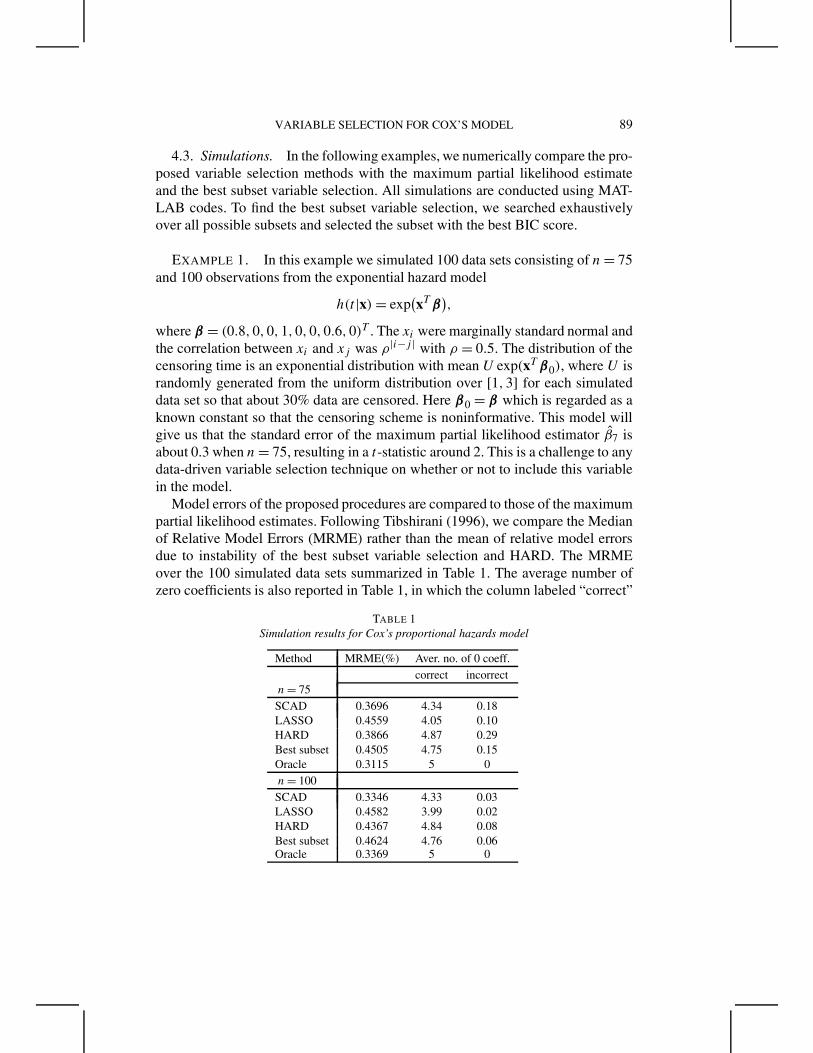
EXAMPLE 1. In this example we simulated 100 data sets consisting of n = 75and 100 observations from the exponential hazard model
h(t|x) = exp(xT β
),
where β = (0.8, 0, 0, 1, 0, 0, 0.6, 0)T . The xi were marginally standard normal andthe correlation between xi and xj was ρ|i−j | with ρ = 0.5. The distribution of thecensoring time is an exponential distribution with mean U exp(xT β0), where U israndomly generated from the uniform distribution over [1, 3] for each simulateddata set so that about 30% data are censored. Here β0 = β which is regarded as aknown constant so that the censoring scheme is noninformative. This model willgive us that the standard error of the maximum partial likelihood estimator β7 isabout 0.3 when n = 75, resulting in a t-statistic around 2. This is a challenge to anydata-driven variable selection technique on whether or not to include this variablein the model.
Model errors of the proposed procedures are compared to those of the maximumpartial likelihood estimates. Following Tibshirani (1996), we compare the Medianof Relative Model Errors (MRME) rather than the mean of relative model errorsdue to instability of the best subset variable selection and HARD. The MRMEover the 100 simulated data sets summarized in Table 1. The average number ofzero coefficients is also reported in Table 1, in which the column labeled “correct”
TABLE 1Simulation results for Cox’s proportional hazards model
Method MRME(%) Aver. no. of 0 coeff.correct incorrect
presents the average restricted only to the true zero coefficients, while the columnlabeled “incorrect” depicts the average of coefficients erroneously set to 0. FromTable 1, the SCAD outperforms the other three methods and performs as well asthe oracle estimator in terms of MRME. All methods select about the same correctnumber of significant variables.
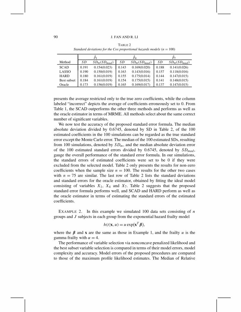
We now test the accuracy of the proposed standard error formula. The medianabsolute deviation divided by 0.6745, denoted by SD in Table 2, of the 100estimated coefficients in the 100 simulations can be regarded as the true standarderror except the Monte Carlo error. The median of the 100 estimated SDs, resultingfrom 100 simulations, denoted by SDm, and the median absolute deviation errorof the 100 estimated standard errors divided by 0.6745, denoted by SDmad ,gauge the overall performance of the standard error formula. In our simulations,the standard errors of estimated coefficients were set to be 0 if they wereexcluded from the selected model. Table 2 only presents the results for non-zerocoefficients when the sample size n = 100. The results for the other two caseswith n = 75 are similar. The last row of Table 2 lists the standard deviationsand standard errors for the oracle estimator, obtained by fitting the ideal modelconsisting of variables X1, X4 and X7. Table 2 suggests that the proposedstandard error formula performs well, and SCAD and HARD perform as well asthe oracle estimator in terms of estimating the standard errors of the estimatedcoefficients.
EXAMPLE 2. In this example we simulated 100 data sets consisting of n
groups and J subjects in each group from the exponential hazard frailty model
h(t|x, u) = u exp(xT β
),
where the β and x are the same as those in Example 1, and the frailty u is thegamma frailty with α = 4.
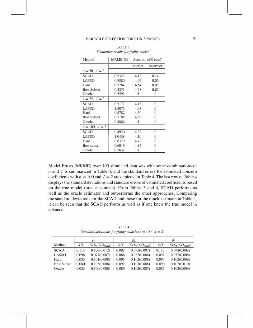
The performance of variable selection via nonconcave penalized likelihood andthe best subset variable selection is compared in terms of their model errors, modelcomplexity and accuracy. Model errors of the proposed procedures are comparedto those of the maximum profile likelihood estimates. The Median of Relative
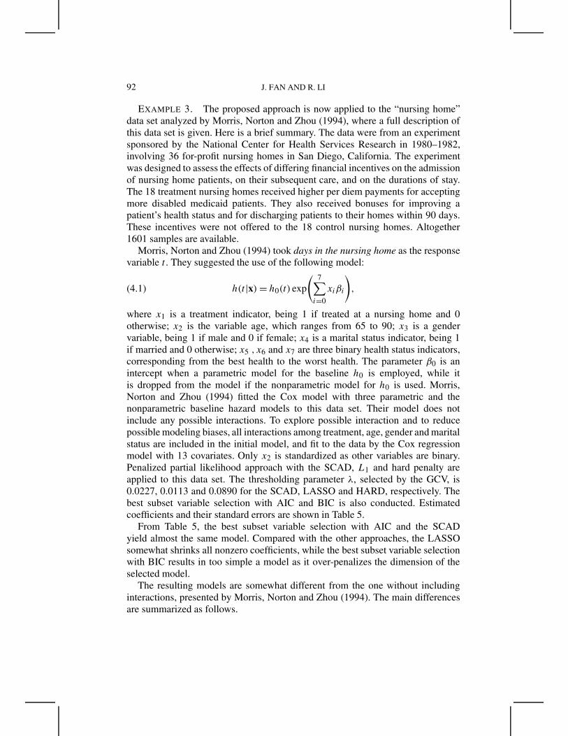
Model Errors (MRME) over 100 simulated data sets with some combinations ofn and J is summarized in Table 3, and the standard errors for estimated nonzerocoefficients with n = 100 and J = 2 are depicted in Table 4. The last row of Table 4displays the standard deviations and standard errors of estimated coefficients basedon the true model (oracle estimate). From Tables 3 and 4, SCAD performs aswell as the oracle estimator and outperforms the other approaches. Comparingthe standard deviations for the SCAD and those for the oracle estimate in Table 4,it can be seen that the SCAD performs as well as if one knew the true model inadvance.
EXAMPLE 3. The proposed approach is now applied to the “nursing home”data set analyzed by Morris, Norton and Zhou (1994), where a full description ofthis data set is given. Here is a brief summary. The data were from an experimentsponsored by the National Center for Health Services Research in 1980–1982,involving 36 for-profit nursing homes in San Diego, California. The experimentwas designed to assess the effects of differing financial incentives on the admissionof nursing home patients, on their subsequent care, and on the durations of stay.The 18 treatment nursing homes received higher per diem payments for acceptingmore disabled medicaid patients. They also received bonuses for improving apatient’s health status and for discharging patients to their homes within 90 days.These incentives were not offered to the 18 control nursing homes. Altogether1601 samples are available.
Morris, Norton and Zhou (1994) took days in the nursing home as the responsevariable t . They suggested the use of the following model:
h(t|x) = h0(t) exp
( 7∑i=0
xiβi
),(4.1)
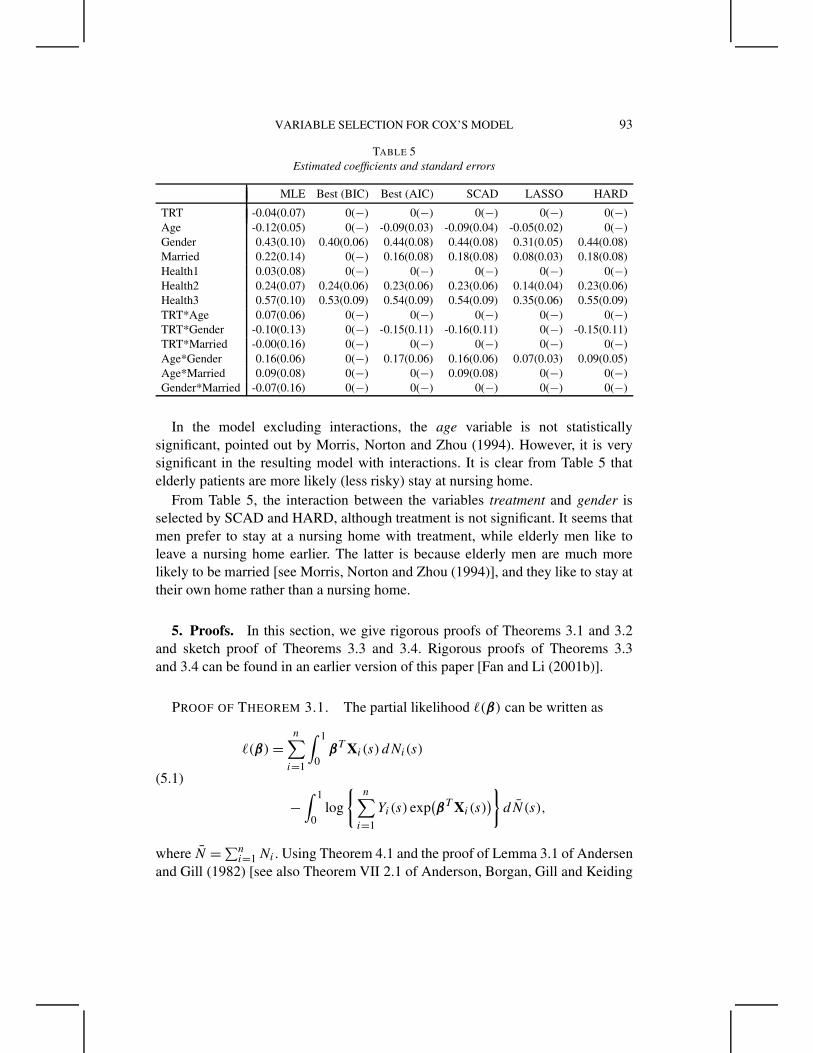
where x1 is a treatment indicator, being 1 if treated at a nursing home and 0otherwise; x2 is the variable age, which ranges from 65 to 90; x3 is a gendervariable, being 1 if male and 0 if female; x4 is a marital status indicator, being 1if married and 0 otherwise; x5 , x6 and x7 are three binary health status indicators,corresponding from the best health to the worst health. The parameter β0 is anintercept when a parametric model for the baseline h0 is employed, while itis dropped from the model if the nonparametric model for h0 is used. Morris,Norton and Zhou (1994) fitted the Cox model with three parametric and thenonparametric baseline hazard models to this data set. Their model does notinclude any possible interactions. To explore possible interaction and to reducepossible modeling biases, all interactions among treatment, age, gender and maritalstatus are included in the initial model, and fit to the data by the Cox regressionmodel with 13 covariates. Only x2 is standardized as other variables are binary.Penalized partial likelihood approach with the SCAD, L1 and hard penalty areapplied to this data set. The thresholding parameter λ, selected by the GCV, is0.0227, 0.0113 and 0.0890 for the SCAD, LASSO and HARD, respectively. Thebest subset variable selection with AIC and BIC is also conducted. Estimatedcoefficients and their standard errors are shown in Table 5.
From Table 5, the best subset variable selection with AIC and the SCADyield almost the same model. Compared with the other approaches, the LASSOsomewhat shrinks all nonzero coefficients, while the best subset variable selectionwith BIC results in too simple a model as it over-penalizes the dimension of theselected model.
The resulting models are somewhat different from the one without includinginteractions, presented by Morris, Norton and Zhou (1994). The main differencesare summarized as follows.
In the model excluding interactions, the age variable is not statisticallysignificant, pointed out by Morris, Norton and Zhou (1994). However, it is verysignificant in the resulting model with interactions. It is clear from Table 5 thatelderly patients are more likely (less risky) stay at nursing home.
From Table 5, the interaction between the variables treatment and gender isselected by SCAD and HARD, although treatment is not significant. It seems thatmen prefer to stay at a nursing home with treatment, while elderly men like toleave a nursing home earlier. The latter is because elderly men are much morelikely to be married [see Morris, Norton and Zhou (1994)], and they like to stay attheir own home rather than a nursing home.
5. Proofs. In this section, we give rigorous proofs of Theorems 3.1 and 3.2and sketch proof of Theorems 3.3 and 3.4. Rigorous proofs of Theorems 3.3and 3.4 can be found in an earlier version of this paper [Fan and Li (2001b)].
PROOF OF THEOREM 3.1. The partial likelihood �(β) can be written as
�(β) =n∑
i=1
∫ 1
0βT Xi (s) dNi(s)
(5.1)
−∫ 1
0log
{n∑
i=1
Yi(s) exp(βT Xi (s)
)}dN(s),
where N =∑ni=1 Ni . Using Theorem 4.1 and the proof of Lemma 3.1 of Andersen
and Gill (1982) [see also Theorem VII 2.1 of Anderson, Borgan, Gill and Keiding
94 J. FAN AND R. LI
(1993)], it follows that under Conditions A–D for each β in a neighborhood of β0,
1
n{�(β) − �(β0)} =
∫ 1
0
[(β − β0)T s(1)(β0, t)
− log
{s(0)(β, t)
s(0)(β0, t)
}s(0)(β0, t)
]h0(t) dt(5.2)
+ OP
( ||β − β0||√n
).
Let αn = n−1/2 +an. It is sufficient to show that for any given ε > 0, there existsa large constant C such that
P
{sup
‖u‖=C
Q(β0 + αnu) < Q(β0)
}≥ 1 − ε.(5.3)
This implies with probability at least 1 − ε that there exists a local maximum inthe ball {β0 + αnu : ‖u‖ ≤ C}. Hence, there exists a local maximizer such that‖β − β0‖ = OP (αn).
Using pλn(0) = 0 and pλn(·) ≥ 0, we have
Dn(u) ≡ 1
n{Q(β0 + αnu) − Q(β0)}
≤ 1
n{�(β0 + αnu) − �(β0)}(5.4)
−s∑
j=1
{pλn(|βj0 + αnuj |) − pλn(|βj0|)},
where s is the number of components of β10. By (5.3) and Taylor’s expansion, wehave
1
n{�(β0 + αnu) − �(β0)}
(5.5)
= −1
2α2
nuT {I (β0) + oP (1)}u + OP
(n−1/2αn‖u‖),
as the first order derivative of the first term in (5.3) equals 0. Since I (β0) is positivedefinite, the first term in the right-hand side of (5.6) is of the order C2α2
n. Note thatn−1/2αn = Op(α2
n). By choosing a sufficiently large C, the first term in the lastequation will dominate the second term, uniformly in ||u|| = C. On the other hand,by the Taylor expansion and the Cauchy–Schwarz inequality, the second term inthe right-hand side of (5.4) is bounded by
√sαnan||u|| + α2
nbn||u||2 = Cα2n
(√s + bnC
)
VARIABLE SELECTION FOR COX’S MODEL 95
which is dominated by the first term of (5.6) as bn → 0, when C is sufficientlylarge. Hence by choosing sufficiently large C, (5.3) holds. This completes the proofof the theorem. �
To establish the oracle property, we show that this estimator must process thesparsity property β2 = 0, which is stated as follows.
LEMMA 5.1. Assume that
lim infn→∞ lim inf
θ→0+ p′λn
(θ)/λn > 0,(5.6)
λn → 0,√
nλn → ∞, and the conditions of Theorem 3.1 hold. Then withprobability tending to 1, for any given β1 satisfying that ‖β1 −β10‖ = OP (n−1/2)
and any constant C,
Q{(
βT1 , 0
)T }= max‖β2‖≤Cn−1/2
Q{(
βT1 ,βT
2)T }
.
PROOF. It is sufficient to show that with probability tending to 1 as n →∞, for any β1 satisfying that β1 − β10 = OP (n−1/2), and ‖β2‖ ≤ Cn−1/2,∂Q(β)/∂βj and βj have different signs for βj ∈ (−Cn−1/2, Cn−1/2) for j =s + 1, . . . , d. From (5.3), for each β in a neighborhood of β0, we have
�(β) = �(β0) + nf (β) + OP
(√n‖β − β0‖
),
where
f (β) =∫ 1
0
[(β − β0)T s(1)(β0, t) − log
{s(0)(β, t)
s(0)(β0, t)
}s(0)(β0, t)
]h0(t) dt.
Note that
∂f (β)
∂β=∫ 1
0
[s(1)(β0, t)
s(0)(β0, t)− s(1)(β, t)
s(0)(β, t)
]s(0)(β0, t)h0(t) dt
and
−∂2f (β)
∂β∂βT=∫ 1
0
[s(2)(β, t)s(0)(β, t)− s(1)(β, t){s(1)(β, t)}T
[s(0)(β, t)]2
]s(0)(β0, t)h0(t) dt.
Thus
f (β0) = 0,∂f (β)
∂β
∣∣∣∣β=β0
= 0
and
− ∂2f (β)
∂β∂βT
∣∣∣∣∣β=β0
= I (β0)
96 J. FAN AND R. LI
which is a finite positive definite matrix. Therefore for each β in a neighborhoodof β0
f (β) = −12 (β − β0)T {I (β0) + o(1)}(β − β0).
By the Taylor expansion, for β in a n−1/2-neighborhood of β0, we have
∂Q(β)
∂βj
= ∂�(β)
∂βj
− np′λn
(|βj |) sgn(βj )
= −n
d∑l=1
∂2f (β0)
∂βj∂βl
(βl − βl0) + OP
(n‖β − β0‖2)− np′
λn(|βj |) sgn(βj )
= −np′λn
(|βj |) sgn(βj ) + OP
(n1/2),
where Ij l(β0) is the (j, l)-element of I (β0). Thus, it follows that
∂Q(β)
∂βj
= nλn
{−λ−1n p′
λn(|βj |) sgn(βj ) + OP
(n−1/2/λn
)}.
Since lim infn→∞ lim infθ→0+ λ−1n p′
λn(θ) > 0 and n−1/2/λn → 0, the sign of the
derivative is completely determined by that of βj . This completes the proof. �
PROOF OF THEOREM 3.2. It follows by Lemma 5.1 that Part (i) holds. Nowwe prove Part (ii). Using the proof of Theorem 3.1, it can be shown that there existsa β1 in Theorem 3.1 that is a root-n consistent local maximizer of Q{(βT
1 , 0)T },satisfying the likelihood equations
∂Q(β)
∂βj
∣∣∣∣β=(βT
1 ,0)T= 0 for j = 1, . . . , s.(5.7)
Let U(β) be the score function of (5.1), that is
U(β) =n∑
i=1
∫ 1
0Xi(s) dNi(s) −
∫ 1
0
∑ni=1 Yi(s)Xi (s) exp{βT Xi(s)}∑n
i=1 Yi(s) exp{βT Xi (s)} dN(s),
and denote
I (β) =∫ 1
0
(∑ni=1 Yi(s)Xi(s)XT (s) exp{βT Xi(s)}∑n
i=1 Yi(s) exp{βT Xi (s)}
− [∑ni=1 YiXi (s) exp{βT Xi(s)}][∑n
i=1 YiXi(s) exp{βT Xi(s)}]T[∑n
i=1 Yi(s) exp{βT Xi (s)}]2
)dN(s).
Note that β1 is a consistent estimator and βj0 �= 0. By Taylor’s expansion, it holdsfor j = 1, . . . , s that
VARIABLE SELECTION FOR COX’S MODEL 97
∂�(β)
∂βj
∣∣∣∣β=(βT
1 ,0)T− np′
λn(|βj |)
= Uj(β0) −s∑
l=1
Ij l(β∗)(βl − βl0)
− n(p′
λn(|βj0|) sgn(βj0) + {p′′
λn(|βj0|) + oP (1)}(βj − βj0)
),
where β∗ is on the line segment between β and β0, Uj (β0) is the j -th componentof U(β0) and Ij l(β
∗) is the (j, l)- element of I (β∗).Using Theorem 3.2 of Andersen and Gill (1982), it can be proved that
1√n
U1(β0) → N{0, I1(β0)}
in distribution as n → ∞, where U1(β0) consists of the first s elements of U(β0),and I1(β10) consists of the first s rows and columns of I (β0); furthermore,
1
nI (β∗) → I1(β0)
in probability as n → ∞. Since β0 = (βT10, 0)T , it follows by using Slutsky’s
Theorem that√
n(I1(β10) + 3){β1 − β10 + (
I1(β10) + 3)−1 b
}→ N
{0, I1(β10)
}.
This completes the proof. �
PROOF OF THEOREM 3.3. Denote αn = n−1/2 + an, and let αn → 0. Itfollows that for any u with ‖u‖ = C, θ 0 + αnu → θ0. Therefore (3.17) holds forθn = θ0 + αnu, which implies that
1
n{log P L(θ0 + αnu) − log P L(θ0)}
= −1
2α2
nuT I0(θ0)u
(5.8)
+ αnuT
n
n∑i=1
�0{(xi1, zi1, δi1), . . . , (xiJ , ziJ , δiJ )}
+ oP
(αn‖u‖ + 1√
n
)2
.
As �0{(xi1, zi1, δi1), . . . , (xiJ , ziJ , δiJ )} is the efficient score function of marginallikelihood of the i-th group data at θ = θ0, the second term of (5.9) is of theorder OP (αn‖u‖/
√n). Note that αn/
√n = OP (α2
n). By choosing sufficient large
98 J. FAN AND R. LI
C, the first term will dominate the second one, uniformly in ‖u‖ = C. Followingthe same strategy as the proof of Theorem 3.1, it can be shown that the results inTheorem 3.3 hold. We omit the details, but see Fan and Li (2001b) for a rigorousproof. �
PROOF OF THEOREM 3.4. The sparsity in Part (i) can be establishedfollowing the same lines in the proof of Lemma 5.1.
Similarly to the proof of Theorem 3.2, it follows by Corollary 1 of Murphy andvan der Vaart (2000) that
in distribution, where I1(θ10) consists of the first (s + 1) × (s + 1) submatrix ofI0(θ10, 0). See Fan and Li (2001b) for a rigorous proof. �
Acknowledgments. The authors would like to thank the referees for construc-tive comments that led to improvement an earlier draft of the paper.
REFERENCES
ANDERSEN, P. K, BORGAN, Ø., GILL, R. D. and KEIDING, N. (1993). Statistical Models Based onCounting Processes. Springer, New York.
ANDERSEN, P. K. and GILL, R. D. (1982). Cox’s regression model for counting processes: a largesample study. Ann. Statist. 10 1100–1120.
ANTONIADIS, A. (1997). Wavelets in Statistics: A review (with discussion). J. Italian Statist. Assoc.6 97–144.
ANTONIADIS, A. and FAN, J. (2001). Regularization of wavelet approximations (with discussion).J. Amer. Statist. Assoc. 96 939–967.
BICKEL, P. J. (1975). One-step Huber estimates in the linear model. J. Amer. Statist. Assoc. 70 428–434.
BREIMAN, L. (1996). Heuristics of instability and stabilization in model selection. Ann. Statist. 242350–2383.
COX, D. R. (1975). Partial likelihood. Biometrika 62 269–276.CRAVEN, P. and WAHBA, G. (1979). Smoothing noisy data with spline functions: estimating the
correct degree of smoothing by the method of generalized cross-validation. Numer. Math.31 377–403.
DONOHO, D. L. and JOHNSTONE, I. M. (1994). Ideal spatial adaptation by wavelet shrinkage.Biometrika 81 425–455.
FAN, J. (1997). Comment on “Wavelets in statistics: a review” by A. Antoniadis. J. Italian Statist.Assoc. 6 131–138.
FAN, J. and LI, R. (2001a). Variable selection via nonconcave penalized likelihood and its oracleproperties. J. Amer. Statist. Assoc. 96 1348–1360.
FAN, J. and LI, R. (2001b). Variable selection for Cox’s proportional hazards model and frailtymodel. Institute of Statistic Mimeo Series #2372, Dept. Statistics, Univ. North Carolina,Chapel Hill.
FARAGGI, D. and SIMON, R. (1998). Bayesian variable selection method for censored survival data.Biometrics 54 1475–1485.
KNIGHT, K. and FU, W. (2000). Asymptotics for lasso-type estimators. Ann. Statist. 28 1356–1378.
VARIABLE SELECTION FOR COX’S MODEL 99
LEHMANN, E. L. (1983). Theory of Point Estimation. Wiley, New York.LI, K. C. (1987). Asymptotic optimality for Cp , Cl , cross-validation and generalized cross
validation: discrete index set. Ann. Statist. 15 958–975.LINDLEY, D. V. (1968). The choice of variables in multiple regression (with discussion). J. Roy.
Statist. Soc. Ser. B 30 31–66.MORRIS, C. N., NORTON, E. C. and ZHOU, X. H. (1994). Parametric duration analysis of nursing
home usage. In Case Studies in Biometry (N. Lange, L. Ryan, L. Billard, D. Brillinger,L. Conquest and J. Greenhouse, eds.) 231–248. Wiley, New York.
MURPHY, S. A. and VAN DER VAART, A. W. (1999). Observed information in semiparametricmodels. Bernoulli 5 381–412.
MURPHY, S. A. and VAN DER VAART, A. W. (2000). On profile likelihood. J. Amer. Statist. Assoc.95 449–465.
NIELSEN, G. G., GILL, R. D., ANDERSEN, P. K. and SØ RENSEN, T. I. A. (1992). A countingprocess approach to maximum likelihood estimator in frailty models. Scand. J. Statist. 1925–43.
PARNER, E. (1998). Asymptotic theory for the correlated gamma-frailty model. Ann. Statist. 26 183–214.
ROBINSON, P. M. (1988). The stochastic difference between econometrics and statistics. Economet-rica 56 531–548.
SINHA, D. (1998). Posterior likelihood methods for multivariate survival data. Biometrics 54 1463–1474.
TIBSHIRANI, R. J. (1996). Regression shrinkage and selection via the lasso. J. Roy. Statist. Soc. Ser.B 58 267–288.
TIBSHIRANI, R. J. (1997). The lasso method for variable selection in the Cox model. Statistics inMedicine 16 385–395.
WAHBA, G. (1985). A comparison of GCV and GML for choosing the smoothing parameter in thegeneralized spline smoothing problem. Ann. Statist. 13 1378–1402.