Variable Techniques - elearningzoom.com · three popular versions of parametric programming:...

Parametric Programming Lesson Two: Variable Techniques

1

Variable Techniques Discussions in lesson one are rather broad in nature. The points made can be applied to any version of parametric programming. From this chapter on, we offer much more specific information. As stated in the preface, discussions and specific examples will be included for three popular versions of parametric programming: Fanuc’s custom macro B, Okuma’s user task 2, and Fadal’s macro.

If you have experience programming with any computer programming language, you already know many of the computer-related functions of parametric programming. However, we do not wish to assume that all readers have written computer programs. For this reason, this chapter begins a lengthy explanation of each computer-related feature. And for now, we keep our presentations in rather basic terms, so even computer programming novices will be able to follow.

We recommend once again that newcomers to computer programming purchase a beginner’s book on BASIC. It will help reinforce your understanding of what can be done with computer-related features of parametric programming. It will also relate much of the mentality that goes into computer programming that is not included in this text, including how to flow-chart the logic related to your more complicated programs. Experienced computer programmers will still need to read the appropriate sections of part one to learn the specific syntax of parametric programming.

What are variables? One of the most important features of parametric programming is the ability to use variables. Though the actual syntax and structure for variables changes from one version of parametric programming to another, the general applications remain remarkably similar.

If you have experience with computer programming, you already know what variables are. The use and application of variables in parametric programming are much the same as they are in any computer programming language. However, most people that have no computer programming experience find it somewhat difficult to understand the concept of variables. For this reason, we begin with two simple analogies to help you understand variables.

Variables are temporary storage locations for numerical values. A value can be placed into a variable for use later. In this sense, you can think of any tool offset as being a kind of variable. With a tool offset, a value is stored in the offset for use by the program. Depending upon the compensation type, the offset value could represent (among other things) the length of a tool, a milling cutter radius, a wear amount, or a turning tool’s nose radius.

With tool length compensation, for example, the programmer includes a command in the program that points to the tool’s tool length compensation offset number. With one popular control, a G43 command specifies tool length compensation is being instated and an H word actually points at the offset number. The command

N015 G43 H02 Z0.1 for example, tells this control to look in offset number two for the tool length compensation value for this tool. Since the programmer will not know the length of each tool as the program is written, they can utilize each of the machine’s tool offsets as a kind of variable. In essence, the


2

programmer is creating a program that will function correctly regardless how long the setup person makes each tool.

At the machine during setup, the setup person will measure the tool length compensation value for tool number two and enter it into tool offset number two. In essence, the setup person is manually assigning the value of a variable that corresponds to tool number two’s length compensation value. This value means nothing to the control until the tool length compensation command (the G43 command in our case) is executed. Note that the value of any variable can be changed whenever it is necessary to do so, just as any tool offset value can be changed at any time. During the production run, for instance, the operator can change the offset value as needed to compensate for tool wear.

To summarize the similarity between offsets and variables, variables are storage locations for values. Like offsets, a value (possibly the result of a calculation) can be stored in the variable. Like offsets, the control will not know the meaning or use of the variable until it is referenced in some way during the execution of the parametric program. And like offsets, most control manufacturers can display the values of all variables right on the display screen. Some even allow certain variables to be entered and/or modified by the CNC operator though the keyboard and display screen.

Variables allow much more flexibility than tool offsets. In almost all cases, a tool offset is used for only one form of compensation, and the compensation type is quite rigid in its use of offsets. With tool length compensation, for example, the offset can only be used to represent the tool length compensation value. If you do not like the way your tool length compensation feature functions, there is nothing you can do about it. On the other hand, a parametric programming variable can be used to represent almost anything. Among the countless things variables can be used to represent are an axis position, an arc radius, a chamfer size, a spindle speed or feedrate, a tool diameter, and almost anything else you can think of. Indeed, your own imagination and ingenuity are the only things that limit what variables can represent.

Variables within parametric programs can also be thought of as memories in an electronic calculator. With a calculator, you can store a value that is needed within your calculations. This memory value can be quickly referenced as required by pressing but one or two keys. Variables within parametric programs can be used to represent constant values (possibly the result of an arithmetic expression) and can be referenced as required within the parametric program. Here are some of the many applications for variables.

• Variables are used to get arguments into the parametric program and tell the program how to behave.

• Variables work as temporary storage locations for values that will be used throughout the parametric program.

• Variables give the programmer the ability to set and step counters.

• Variables give the programmer the ability to set flags.

• Variables can be used as constant values that seldom change. Most programmers that program in the inch mode, for example, use a value of 0.100 in as their rapid approach distance. If programmed as a hard-and-fixed value, it can be quite difficult to change all approaches in the program to something


3

smaller - say 0.050 in - to reduce cycle time. However, if this approach distance is specified as a variable and referenced during every approach, the approach distance can be easily changed by changing one word in the program.

As with any computer programming language, there are different types of variables with most versions of parametric programming. While most versions of parametric programming do not require that you declare the variable type as you must in some computer programming languages, the parametric programmer must understand the different types available with their particular version in order to write parametric programs.

Variables in Fanuc’s custom macro B There are five types of variables in custom macro B. With but one exception, all variables in custom macro B are represented by a pound sign (#) and a number. The number next to the pound sign specifies the variable number and also implies its type.

Arguments and local variables As stated, arguments specify values that change from one execution of the custom macro the next. They tell the custom macro program how to behave right now, and are especially helpful in user-created canned cycle and family-of-parts applications. There are actually two ways in custom macro B to use arguments, based on which of these two these application categories you are working with.

Arguments with user created canned cycle applications With user created canned cycles, it is almost always best to specify arguments in a G65 command, as briefly introduced in chapter one. Since user created canned cycles only machine a small portion of the workpiece, and since they may have to be executed several times by the main program, G65 makes a very convenient way of getting data into the custom macro since it resembles a canned cycle command. Within the G65, a P word is included to specify the program number of the custom macro program. Then comes the list of arguments. Here is a list of argument letter addresses allowed in custom macro B.

A, B, C, D, E, F, H, I, J, K, M, Q, R, S, T, U, V, W, X, Y, and Z Note that not all letters of the alphabet are allowed as arguments. G, L, N, O, and P are missing. You must choose from those letter addresses that are allowed by custom macro. For reasons we will discuss much later, we also recommend avoiding I, J, and K.

Though not all letters are allowed as arguments, custom macro B gives the parametric programmer remarkable flexibility with argument naming. In most cases, a very logical argument name can be chosen (A for angle, R for radius, T for tool, D for depth, and so on). If programming for user created canned cycle applications with custom macro B, you’ll want to take advantage of this argument naming flexibility.

One important point about letter address arguments is that you should include a decimal point with each argument value specified in the G65 command. Without the decimal point, the control will use the fixed format for the letter address word to interpret the argument value. As you probably know, this fixed format changes from one word type to another. The letter address X, for example, has a four place decimal format in the inch mode. If the decimal point is left out, a value of X1 will be taken as X0.0001 on most controls. However, the letter address B has a three place format. A value of B1 (without the decimal point) will be taken as B0.001. In order to


4

avoid any confusion regarding the placement of the decimal point for each word, be sure to specify the decimal point in all arguments included in the G65 command.

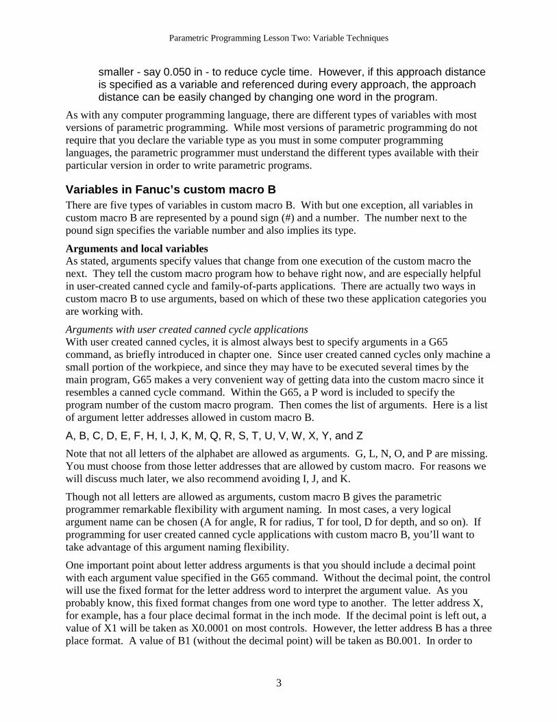
Figure 2.1

Figure 2.1 shows an example of a very simple application. We limit our discussion at this time to argument name selection and will not (as yet) show the actual custom macro program. Notice that the right side of this workpiece must be milled. Based on knowing the company’s work, the programmer knows that this is but one of over 300 workpieces that requires the right side to be milled. Rather than writing the redundant coding needed to mill the right side in over 300 programs, the programmer wishes to write a user defined canned cycle to do the milling.


5

Figure 2.2

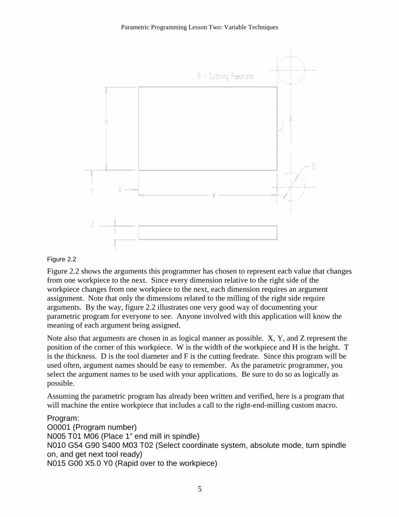
Figure 2.2 shows the arguments this programmer has chosen to represent each value that changes from one workpiece to the next. Since every dimension relative to the right side of the workpiece changes from one workpiece to the next, each dimension requires an argument assignment. Note that only the dimensions related to the milling of the right side require arguments. By the way, figure 2.2 illustrates one very good way of documenting your parametric program for everyone to see. Anyone involved with this application will know the meaning of each argument being assigned.

Note also that arguments are chosen in as logical manner as possible. X, Y, and Z represent the position of the corner of this workpiece. W is the width of the workpiece and H is the height. T is the thickness. D is the tool diameter and F is the cutting feedrate. Since this program will be used often, argument names should be easy to remember. As the parametric programmer, you select the argument names to be used with your applications. Be sure to do so as logically as possible.

Assuming the parametric program has already been written and verified, here is a program that will machine the entire workpiece that includes a call to the right-end-milling custom macro.

Program: O0001 (Program number) N005 T01 M06 (Place 1” end mill in spindle) N010 G54 G90 S400 M03 T02 (Select coordinate system, absolute mode, turn spindle on, and get next tool ready) N015 G00 X5.0 Y0 (Rapid over to the workpiece)


6

N020 G43 H01 Z0.1 (Instate tool length compensation, move up close to work surface) N025 G65 P1000 X0. Y0. Z0. W5.0 H3.0 T0.5 D1.0 F5.0 (Mill right side) N030 G91 G28 Z0 M19 (Move to tool change position, orient spindle) N035 M01 (Optional stop) N040 T02 M06 (Place 1/2 drill two in spindle) N045 G54 G90 S800 M03 T01 (Select coordinate system, absolute mode, start spindle, get tool number one ready) N050 G00 X0.5 Y0.5 (Rapid to first hole position) N055 G43 H02 Z0.1 (Instate tool length compensation, rapid up close to work surface) N060 G81 R0.1 Z-0.85 F4.0 (Drill first hole) N065 Y2.5 (Drill second hole) N070 X4.5 (Drill third hole) N075 Y0.5 (drill fourth hole) N080 G80 (Cancel cycle) N085 G91 G28 Z0 M19 (Return to tool change position, orient spindle) N090 M30 (End of program) Once again, note how little of this program actually deals with the milling of the right side. Only one command is involved (line N025). If more workpieces must be milled by this program, it is easy to simply specify more calling commands (G65) to program number O1000.

You must be exposed to another variable type (local variables) before we can show the custom macro that actually does the machining for this application. Local variables will be discussed just a little later.

Arguments with family-of-parts applications While G65 is a very helpful command, and it is almost always the method of choice for user-created canned cycle applications, it is not always the most convenient way to get data into the custom macro. When programming family-of-parts applications, for example, the entire workpiece is being machined by the parametric program. In this case, it is usually more convenient to state the values of all arguments at the beginning of the program rather than call the parametric program from another program. This involves using another of the custom macro variable types. Common variables can be used for this purpose.

Common variables range in the #100 series. At least fifty common variables are available (more can be purchased as an option) and they range from #100 through (at least) #149. (More on common variables a little later.) Though the naming of each argument must be well documented, common variables make better arguments with family-of-part applications. We will again use the workpiece in figure 2.1 as for the example program, but will change the criteria of the application. Instead of just milling the right end for a variety of different workpieces, say the workpiece shown in figure 2.1 is but one of over 100 very similar workpieces. All workpieces have the four 1/2” diameter holes drilled through the workpiece 0.5 in from each edge. This new criteria (machining the entire workpiece) changes the application from a user-created canned cycle application to a family-of-parts application. Figure 2.3 shows the documentation for this application, including the needed common variable arguments.


7

Figure 2.3

Notice that the argument names themselves (#100 - #108) now mean nothing. There is no way to relate the 100 series number to the workpiece attribute it represents. For this reason, argument meanings must be clarified in the program (as shown in our example program) as well as in any supporting documentation for this program. Here is the custom macro program that machines all workpieces in this part family.

O0002 (Program number) (Argument assignments) #100 = 0 (Left side position in X) #101 = 0 (Lower side position in Y) #102 = 0 (Top surface of workpiece in Z) #103 = 5.0 (Length of workpiece in X) #104 = 3.0 (Width of workpiece in Y) #105 = 0.5 (Workpiece thickness) #106 = 1.0 (Milling cutter diameter) #107 = 400 (RPM for milling cutter) #108 = 5.0 (Feedrate of milling cutter in IPM) (Machining portion of the program) N005 T01 M06 (Place 1” end mill in spindle) N010 G54 G90 S#107 M03 T02 (Select coordinate system, absolute mode, turn spindle on, and get next tool ready) N015 G00 X[#100 + #103 + #106/2] Y[#101 - 0.1 - #106/2] (Rapid over to the workpiece)


8

N020 G43 H01 Z[#102 + 0.1] (Instate tool length compensation, move up close to work surface) N025 G01 Z[#102 - #105 - 0.1] F50.0 (Fast feed past surface) N030 Y[#101 + #104 + 0.1 +#106/2] F#108 (Mill right side) N035 G00 Z[#102 + 0.1] (Rapid to above top surface) N035 G91 G28 Z0 M19 (Move to tool change position, orient spindle) N040 M01 (Optional stop) N045 T02 M06 (Place 1/2 drill two in spindle) N050 G54 G90 S800 M03 T01 (Select coordinate system, absolute mode, start spindle, get tool number one ready) N055 G00 X[#100 + 0.5] Y[#101 + 0.5] (Rapid to first hole position) N060 G43 H02 Z[#102 + 0.1] (Instate tool length compensation, rapid up close to work surface) N065 G81 R[#102 + 0.1] Z[#102 - #105 - 0.18] F4.0 (Drill first hole) N070 Y[#101 + #104 - 0.5] (Drill second hole) N075 X[#100 + #103 - 0.5] (Drill third hole) N080 Y[#101 + 0.5] (drill fourth hole) N085 G80 (Cancel cycle) N090 G91 G28 Z0 M19 (Return to tool change position, orient spindle) N095 M30 (End of program) Since this is the first full parametric programming example we have shown, it bares further explanation. First of all, notice how well arguments #100 through #108 are documented in the program. A message in parentheses is placed next to each argument to tell anyone viewing this program exactly what each argument means. An operator or setup person could confidently modify one or more of these arguments during setup for the next workpiece in the family to be machined without fear of making mistakes.

Second, notice that arguments are only required for those things that change from one workpiece in the family to the next. Any value that does not change (speed and feed for 1/2” drill, 0.5 inch hole position, 0.1” approach distance, etc.) is treated as a constant value. Constant values, of course, cannot be changed by simply manipulating argument values.

Third, notice that calculations are being done in many of this program’s commands to determine axis positions. While arithmetic functions are discussed in detail in chapter three, it is almost impossible to come up with any good parametric programming example that does not require them. Look specifically at line N015. The X and Y positioning movements will be based on the result of a calculation. Based on the current values of the arguments set at the beginning of this program, the X value will be calculated as 5.5 (0 + 5.0 + 1.0 / 2). The Y value will be calculated as -0.6 (the negative result of 0.1 + 1.0 / 2). When executed, this command will appear to the control as “N015 G00 X5.5 Y-0.6”. Keep in mind, however, that if the values of #100, #103, and/or #106 are changed (as will be necessary for other workpieces in the family), the positioning movement in line N015 will also change.

Finally, notice the brackets ([]) that enclose the calculations being made to determine the value of a CNC word. These brackets are not parentheses. Custom macro B requires that brackets be used in this manner when making calculations to determine the value of CNC words. More on brackets during our discussion of arithmetic functions.


9

While this is a relatively simple family-of-parts application, it should nicely stress how arguments can be introduced to family-of-parts parametric programs. Though we are just scratching the surface of what can be done, it should also begin to show you some of the power you have available with parametric programming.

Please note once more the subtle distinction between argument assignment for user-created canned cycle applications and argument assignment for family-of-parts applications. With part families, the custom macro is machining the entire workpiece, and assigning arguments in the main program is usually the most convenient method of argument assignment since only one program is required.

On the other hand, since user-created canned cycle applications always require a separate program to perform the canned-cycle-like operation, and since this program may be required several times even to machine one workpiece, arguments must be set in the main program (within the G65 command). And it must be possible to manipulate the arguments from one call statement to the next.

Local variables with argument assignment number one

As you now know, when a custom macro is called with a G65 command, argument values are passed in the form of letter addresses. As stated earlier, legal letter address arguments include:

A, B, C, D, E, F, H, I, J, K, M, Q, R, S, T, U, V, W, X, Y, and Z Though it may seem a little confusing at first, you are not allowed to directly reference an argument within the custom macro by its letter address. The control would confuse the argument name (A, B, C, X, Y, Z, etc.) with the true CNC meaning for the letter address. For this reason, you must reference arguments by their corresponding local variables. Here is a list that shows all letter address arguments and their corresponding local variable numbers. This is the most popular form of argument assignment, called argument assignment number one.

A:#1, B:#2, C:#3, D:#7, E:#8, F:#9, H:#11, I:#4, J:#5, K:#6, M:#13, Q:#17, R:#18, S:#19, T:#20, U:#21, V:#22, W:#23, X:#24, Y:#25, Z:#26

When a G65 command is executed, two things will happen. First, all local variables that have corresponding letter address arguments in the G65 command will be set. Second, the custom macro specified by the P word will be executed. During the execution of the custom macro, local variables will contain the values of arguments set in the G65 command. Within the custom macro, these local variables must be used to reference the arguments coming from the G65 calling command.

As an example, the command

N025 G65 P1000 X0. Y0. Z0. W5.0 H3.0 T0.5 D1.0 F5.0 (Mill right side) first sets the local variables corresponding to X, Y, Z, W, H, T, D, and F. In this case, local variable #24 will be set to 0 (the X value), #25 to 0 (the Y value), #26 to 0 (the Z value), #23 to 5.0 (the W value), #11 to 3.0 (the H value), #20 to 0.5 (the T value), #7 to 1.0 (the D value), and #9 to 5.0 (the F value). Then the control executes program O1000. When the programmer wishes to reference the value of X within the custom macro program, #24 must be used.

It is also important to know that all other local variables (#1, #2, #3, etc.) will have no value when the custom macro is executed, meaning they will be left vacant. Do not confuse vacant


10

with zero. Zero is a value. When a variable is vacant, it has no value. We will discuss some implications of vacant variables later.

Also note that, as the name implies, local variables only remain set during the execution of the custom macro. At the completion of the custom macro (the M99 command), they are all set back to vacant.

Here is a full example that uses the workpiece shown in figure 2.1. Again, we are milling the right side of the workpiece, and the arguments used for this user-created canned cycle application are shown in figure 2.2. Here is the main program that machines the workpiece in the same form shown earlier in this chapter.

Program:

O0001 (Program number) N005 T01 M06 (Place 1” end mill in spindle) N010 G54 G90 S400 M03 T02 (Select coordinate system, absolute mode, turn spindle on, and get next tool ready) N015 G00 X5.0 Y0 (Rapid over to the workpiece) N020 G43 H01 Z0.1 (Instate tool length compensation, move up close to work surface) N025 G65 P1000 X0. Y0. Z0. W5.0 H3.0 T0.5 D1.0 F5.0 (Mill right side) N030 G91 G28 Z0 M19 (Move to tool change position, orient spindle) N035 M01 (Optional stop) N040 T02 M06 (Place 1/2 drill two in spindle) N045 G54 G90 S800 M03 T01 (Select coordinate system, absolute mode, start spindle, get tool number one ready) N050 G00 X0.5 Y0.5 (Rapid to first hole position) N055 G43 H02 Z0.1 (Instate tool length compensation, rapid up close to work surface) N060 G81 R0.1 Z-0.85 F4.0 (Drill first hole) N065 Y2.5 (Drill second hole) N070 X4.5 (Drill third hole) N075 Y0.5 (drill fourth hole) N080 G80 (Cancel cycle) N085 G91 G28 Z0 M19 (Return to tool change position, orient spindle) N090 M30 (End of program) Again, note that line N025 will perform the milling of the right side. Armed with your new knowledge of local variables, you should now be able to understand the custom macro program.

O1000 (Custom macro to mill right side) N1 G00 X[#24 + #23 + #7/2] Y[#25 - 0.1 - #7/2] (Rapid to starting position) N2 G01 Z[#26 - #20 - 0.1] F50. (Fast feed to work surface) N3 Y[#25 + #11 + #7/2] F#9 (Mill right side) N4 G00 Z[#26 + 0.1] Rapid to above workpiece) N5 M99 (End of custom macro) In line N1, with the call statement set as it is in line N025 of the main program, the X position will be calculated as X5.5 because argument X (referenced by #24) is set to 0, W (referenced by #23) is set to 5.0, and D (referenced by #7) is set to 1.0. The control will calculate this X position as 0 + 5.0 + 1.0/2 which results in a value of 5.5.


11

Keeping track of local variables Admittedly, local variable numbers do not make much sense in argument assignment number one. Even for experienced custom macro programmers, it is difficult to remember which local variable corresponds to a given letter address argument. For this reason, you must keep the argument assignment list shown earlier handy as you write custom macros.

One helpful suggestion is to write the letter address argument (in a different color) next to the local variable number as you actually write the custom macro program. For example, say you must reference the letter address argument D in the custom macro. As you look at the local variable assignment list, you find that #7 corresponds to D. As you write #7 in the custom macro, also write the letter “D” in a different color close by to remind you of which letter address argument #7 represents.

Running out of variables? While local variables are used predominantly to represent letter address arguments coming from the G65 command, there is nothing that prohibits you from using unused local variables for other purposes. The next discussion describes common variables. Almost anything that can be done with a common variable can also be done with an unused local variable. The exception to this statement is any application that requires the value of the variable to be retained after the completion of the custom macro (after the M99). Of course, local variables are reset to vacant at M99.

More on vacancy Remember that when a letter address argument is left out of the call statement, its corresponding local variable is set to vacant when the custom macro is called by the G65 command. The custom macro representation for vacancy is #0. Though we do not wish to dig in too deep yet, there are several times when it can be helpful to know about vacant local variables.

In the previous right-side-milling custom macro, for example, all arguments shown in figure 2.2 must be included in the G65 command. By the way, we call arguments that must be included in the call statement mandatory arguments. In our example, all arguments are mandatory arguments. Based on the way the custom macro is written (shown earlier), if the programmer using this custom macro forgets to include one or more of the arguments in the G65 command, it will be difficult to predict what will happen. Surely the custom macro will not behave as expected.

However, by knowing that a local variable is left set to vacant (#0) if it is not included in the call statement, and by knowing how to perform tests in the custom macro (shown in chapter four), the custom macro programmer can test all local variables being assigned to determine if any are vacant. If so, an alarm can be generated to halt the machine before any damage can be done. We will show how to perform tests and generate alarms in chapter four. And this is but one of several times when understanding variable vacancy can be helpful.

Common variables Common variables have been introduced during our discussion of arguments used in family-of-parts applications. Again, common variables range in the #100 series and at least fifty are available (from #100 through #149). More can be purchased as an option.

As the name implies, common variables remain active even after the execution of the custom macro program. Most CNC controls that have custom macro are set to retain the values of


12

common variables (#100 series) until the power to the machine is turned off, at which time they are set back to vacant.

While the global nature of common variables have special implications, for now, we will concentrate on the more basic uses for common variables. Aside from being used as arguments in family-of-parts applications, common variable have a variety of applications.

To minimize redundant calculations

In the simple right-end-milling custom macro application shown earlier, the diameter of the endmill is passed to the custom macro (with D). Yet in the custom macro, it is necessary to utilize the endmill’s radius. The redundant calculation “#7/2” is done three times in this custom macro. While this is a simple calculation and is only performed three times, imagine that the end mill is being used to machine several surfaces. In this cases, it is likely that the expression #7/2 would be stated many times. These calculations are tedious and error prone to write, and force the control to perform unnecessary calculations. This can result in wasted execution (cycle) time.

Common variables can be used to minimize redundant calculations. The result of a redundant calculation can be stored into a common variable early on in the custom macro. From this point, the variable can be used instead of the repeated calculation. Here is the custom macro program to mill the right side of a workpiece modified to take advantage of this technique.

O1000 (Custom macro to mill right side) N1 #100 = #7/2 N2 G00 X[#24 + #23 + #100] Y[#25 - 0.1 - #100] (Rapid to starting position) N3 G01 Z[#26 - #20 - 0.1] F50. (Fast feed to work surface) N4 Y[#25 + #11 + #100] F#9 (Mill right side) N5 G00 Z[#26 + 0.1] Rapid to above workpiece) N6 M99 (End of custom macro) For general purpose calculations Common variables are typically the variable type of choice for general purpose calculations that must be done in the custom macro. Here is another version of the right-side-milling custom macro that calculates all positioning movements up-front, storing the results of all calculations in common variables. The movement commands simply reference the values previously calculated.

O1000 (Custom macro to mill right side) N1 #100 = #24 + #23 + #7/2 N2 #101 = #25 - 0.1 - #7/2 N3 #102 = #26 - #20 - 0.1 N4 #103 = #25 + #11 + #7/2 N5 #104 = #26 + 0.1 N2 G00 X#100 Y#101 (Rapid to starting position) N3 G01 Z#102 F50. (Fast feed to work surface) N4 Y#103 F#9 (Mill right side) N5 G00 Z#104 Rapid to above workpiece) N6 M99 (End of custom macro) As you develop your own custom macros, there will be many times when you use common variables for general purpose calculations.


13

As counters Looping functions often require that variables change each time the loop is executed. Though loops have yet to be introduced (in chapter four), common variables will be used as the loop counter and any other variable that must be initialized at the beginning of the loop and stepped each time through the loop.

As flags It is sometimes necessary to set a flag that tells the custom macro how to behave. For example, you may wish to set up criteria in your right-side milling custom macro that allows the milling cutter to either climb or conventional mill. A special flag will specify which milling method you wish to use. In essence, you are flagging the custom macro as to how it should behave. Other examples of when flags are required (that we will discuss in greater detail during our discussion of conditional branching in chapter four) include right hand versus left hand tooling, inch versus metric input, and whether or not coolant is to be used. While letter address arguments in the G65 command commonly set flags, the global nature of common variables makes it possible to maintain the values of flags even among several programs.

Permanent common variables These variables range in the #500 series. Ten are standard (from #500 through #509) and more permanent common variables can be purchased as an option. As the name implies, these variables are retained even after the power is turned off. In this sense, they are much like tool offsets. And like tool offsets, most controls even let you modify the values of permanent common variables through the keyboard and display screen.

Since there are so few permanent common variables in many controls, it is wise to reserve their use for those applications when it is necessary to retain data from one day to the next. One example of when this is necessary is a utility custom macro for part counting. Say you wish to set up a part counter to let the machine run 750 workpieces and then halt the machine (this application is shown in detail later). As you begin running production, your custom macro based part counter will begin counting workpieces.

It isn’t very likely that you will finish all 750 workpieces before the end of the day/shift. It will be more likely that it will take several days to complete the production run. In this case, you will need your part counting custom macro program to remember where it left off from day to day. If you store the current part count in a #500 series permanent common variable, the value of the variable will not be lost when the power is turned off.

Do you have a probing system? Permanent common variables are also used to retain system data when certain accessory devices are used. If you have a probing system, for example, and if custom macro is used to program the probe, it is quite likely that at least some of your permanent common variables are being used to store calibration values for the probing system. Before you begin using any #500 series permanent common variables, you must confirm that they are not already being used for other purposes.

Setting your own system constants Think of any constant hard-and-fixed value that you use throughout your CNC programming. One that may come to mind is your rapid approach and retract distance. When programming in the inch mode, for example, many programmers like to stay a constant 0.100 in away from the


14

surface being approached before entering a cutting mode. When cutting is completed, many programmers feed the tool away from the workpiece by this same 0.100 in amount.

While this approach distance is quite safe, when high production quantities must be run, the time each approach and retract at the cutting feedrate adds to cycle time may be excessive. However, if all approach and retract movements are programmed with hard-and-fixed values (calculated by the programmer), it can be quite difficult to change the approach and retract values without a massive overhaul of the CNC program.

If instead, a permanent common variable is used in which to store the rapid approach and retract distance (you could even use one permanent common variable for each), and if this variable is referenced in every CNC program during every tool’s approach and retract movement, changing the approach/retract distance will be as simple as changing one permanent common variable. And as stated, permanent common variables can be entered and changed through the keyboard and display screen, just like tool offsets.

Consider this program that drills a few holes and mills a slot. It assumes the rapid approach/retract distance is stored in permanent common variable #500.

O0003 (Program that allows easy approach/retract distance change) N005 T01 M06 (Place 1/2 drill in spindle) N010 G54 G90 S800 M03 T02 (Select coordinate system, absolute mode, turn spindle on, and get tool number two ready) N015 G00 X.5 Y.5 (Rapid to first hole location) N020 G43 H01 Z#500 (Instate tool length compensation, rapid up to workpiece) N025 G81 R#500 Z-.85 F3.5 (Drill first hole) N030 Y3.5 (Drill second hole) N035 X4.5 (Drill third hole) N040 Y.5 (Drill fourth hole) N045 G80 (Cancel cycle) N050 G91 G28 Z0 (Return to tool change position) N055 M01 (Optional stop) N060 T02 M06 (Place 3/8 drill in spindle) N065 G54 G90 S950 M03 T03 (Select coordinate system, absolute mode turn spindle on and get tool three ready) N075 G00 X3.0 Y2.0 (Rapid to hole location) N080 G43 H02 Z#500 (Instate tool length compensation, rapid to approach position) N085 G81 R#500 Z-.55 F3.5 (Drill hole) N090 G80 (Cancel cycle) N095 G91 G28 Z0 (Return to tool change position) N100 M01 (Optional stop) N105 T03 M06 (Place 1/4” endmill in spindle) N110 G54 G90 S1000 M03 T01 (Select coordinate system, absolute mode turn spindle on and get tool one ready) N115 G00 X3.75 Y-[.125 + #500] (Rapid to slot approach position) N120 G43 H03 Z-0.125 (Instate tool length compensation, rapid to work surface) N125 G01 Y[4.125 + #500] F2.5 (Mill slot) N130 G00 Z#500 (Rapid to above work surface) N135 G91 G28 Z0 (Return to tool change position)


15

N140 M30 (End of program) Notice that any time a tool in this program approaches or retracts (lines N020, N025, N080, N085, N115, N125, and N130), permanent common variable #500 is referenced. In lines N115 and N125, notice how the programmer can even perform a calculation that has the control figure out the correct approach/retract position based on the value of permanent common variable #500. With this program, changing the approach/retract distance will be as easy as changing #500.

System variables Many of the CNC related features of custom macro are handled with system variables. These variables range from #1000 through about #6000. They allow access to many CNC functions including current machine position, offsets, alarm generation, and much more. These variables will be well covered in chapter five.

Summary of custom macro variables As you have seen, there are five types of variables in custom macro B. Arguments are used in family-of-parts and user-created canned cycle applications to get input data into the custom macro. Local variables, which get reset to vacant at the completion of the custom macro (at M99), are used to represent letter address arguments coming from the G65 command. Common variables, which can also be used as arguments (in family-of-parts applications), are used for a variety of purposes including general purpose calculations, counters, and minimizing redundant calculations. Permanent common variables are used for applications which require that the value of a variable is retained from day to day. And system variables which allow access to many CNC related features of custom macro. While you should have a pretty good idea of what custom macro variables can do, remember that all presentations to this point have been rather elementary. There are some advanced implications yet to be discussed. We will address these advanced implications in future chapters.

Variables in Okuma’s user task 2 There are three types of variables in user task 2. If you have read the previous section about variables in Fanuc’s custom macro B, the same kinds of functions are available. Only the terminology and syntax changes.

Actually, Okuma does name variables in user task 2 in the same manner as variables are named in custom macro B; local variables, common variables, and system variables. However, there are subtle differences in usage which may lead to confusion if your are working with both of these powerful versions of parametric programming.

Local variables As the name implies, local variables will remain active only during the execution of the user task program. At the completion of the program (or when the control is reset), local variables are cleared. 127 local variables are available with most control models.

Local variable names are chosen by the user task programmer. While there are some strict rules about local variable naming, this ability to name your own local variables allows you to choose very logical local variable names. Local variable names can be up to four characters long. The first two characters (which are mandatory) must be letters of the alphabet. The next two characters can be letters or numbers. The letters O, N, and V cannot be used in a local variable name. Examples of acceptable local variable names include DIA1, THRD, FLG1, XY, and


16

AB11. You will want to take advantage of this flexible local variable naming ability as you develop user task programs to keep variable names as logical and easily to remember as possible.

Using local variables as arguments We call any variable that passes data into the user task program an argument. In most cases, local variable can be used for this purpose.

Local variable arguments for user created canned cycle applications In most user-created canned cycle applications, a CALL command will be used to pass arguments and activate the user task program. The CALL command will include the program name being called and a list of arguments (local variables) to be passed to the user task program.

Figure 2.4

Figure 2.4 shows an example of a very simple application. Notice that the right side of this workpiece must be milled. Based on knowing the company’s work, the programmer knows that this is but one of over 300 workpieces that requires the right side to be milled. Rather than writing the code needed to mill the right side in over 300 programs, the programmer wishes to write a user defined canned cycle to do the milling.


17

Figure 2.5

Figure 2.5 shows the local variable arguments one programmer has chosen to represent each value that changes from one workpiece to the next. Since every dimension relative to the right side of the workpiece changes from one workpiece to the next, each dimension requires an argument assignment. Note that only the dimensions related to the milling of the right side require arguments. By the way, figure 2.5 illustrates one very good way of documenting your parametric program for everyone to see. Anyone involved with this application will know the meaning of each local variable argument being assigned.

Note also that arguments are chosen in as logical manner as possible. XZER, YZER, and ZZER represent the position of the corner of this workpiece. WIDT is the width of the workpiece and HGHT is the height. THK is the thickness. TDIA is the tool diameter and FEED is the cutting feedrate. Since this program will be used often, argument names should be easy to remember. As the parametric programmer, you select the argument names to be used with your applications. Be sure to do so as logically as possible.

Assuming the parametric program has already been written and verified, here is a program that will machine the entire workpiece that includes a call to the right-end-milling user task program.

Program:

O0001 (Program name) N005 G15 H01 (Select coordinate system) N010 T01 M06 (Place 1” end mill in spindle) N015 G90 S400 M03 T02 (Select absolute mode, turn spindle on, and get next tool ready)


18

N020 G00 X5.0 Y0 (Rapid over to the workpiece) N025 G56 H01 Z0.1 (Instate tool length compensation, move up close to work surface) N030 CALL O1000 XZER = 0 YZER = 0 ZZER = 0 WIDT = 5.0 HGHT = 3.0 THK = 0.5 TDIA = 1.0 FEED = 5.0 (Mill right side) N035 G15 H01 (Select coordinate system) N040 G00 Z50.0 (Move to tool change position) N045 T02 M06 (Place 1/2 drill two in spindle) N050 G90 S800 M03 T01 (Select absolute mode, start spindle, get tool number one ready) N055 G00 X0.5 Y0.5 (Rapid to first hole position) N060 G56 H02 Z0.1 (Instate tool length compensation, rapid up close to work surface) N065 G81 R0.1 Z-0.85 F4.0 (Drill first hole) N070 Y2.5 (Drill second hole) N075 X4.5 (Drill third hole) N080 Y0.5 (drill fourth hole) N085 G80 (Cancel cycle) N090 G00 Z50. (Move away in Z) N095 M02 (End of program) Note how little of this program deals with the milling of the right side. Only one command is involved (line N030). If more workpieces must be milled by this program, it is easy to simply specify more calling commands (with more CALL commands) to the program named O1000.

Here is the user task program that actually mills the right side. Notice how easy it is to directly reference the value of each argument (local variable) being set in the main program.

O1000 (User task program to mill right side) N1 G00 X=XZER+WIDT+TDIA/2 Y=YZER-0.1-TDIA/2 (Rapid to starting position) N2 G01 Z=ZZER-THK-0.1 F50. (Fast feed to work surface) N3 Y=YZER+HGHT+TDIA/2 F=FEED (Mill right side) N4 G00 Z=ZZER+0.1 Rapid to above workpiece) N5 RTS (End of user task program) While this user task program should be relatively easy to follow, there are a few points we wish to make about its structure. First of all, notice that each local variable argument is being referenced exactly as it is named in the CALL command from the main program. Second, notice that each actual CNC word that relates to a local variable includes an equal sign (=) to set the word equal to the local variable or calculation result. Finally, notice that arithmetic calculations are being done within several commands. While these simple arithmetic functions should be quite understandable, we will discuss the arithmetic functions of user task 2 in detail later.

Local variables for family-of-parts applications While the CALL command is very helpful, and it is almost always the method of choice for user-created canned cycle applications, it is not always the most convenient way to get data into the user task program. When programming family-of-parts applications, the entire workpiece is being machined by the parametric program. In this case, it is usually more convenient to state the values of all local variable arguments at the beginning of the program rather than to call the user task program from another program.


19

We will again use the workpiece in figure 2.4 as for the example program, but will change the criteria of the application. Instead of just milling the right side for a variety of different workpieces, say the workpiece shown in figure 2.4 is but one of over 100 very similar workpieces. All workpieces have four 1/2” diameter holes drilled 0.5 in from each edge. This new criteria (machining the entire workpiece) changes the application from a user-created canned cycle application to a family-of-parts application. Again, figure 2.5 shows the local variable arguments related to this application. Since the hole locations are always 1/2” in diameter and 0.5 in from the edges, no additional local variable arguments are required. Here is the user task program that machines all workpieces in this part family.

Program:

O0002 (Program name) (Argument assignments) XZER = 0 (Left side position in X) YZER = 0 (Lower side position in Y) ZZER = 0 (Top surface of workpiece in Z) WIDT = 5.0 (Length of workpiece in X) HGHT = 3.0 (Width of workpiece in Y) THK = 0.5 (Workpiece thickness) TDIA = 1.0 (Milling cutter diameter) FEED = 5.0 (Feedrate of milling cutter in IPM) (Machining portion of the program) N005 G15 H01 (Select coordinate system) N010 T01 M06 (Place 1” end mill in spindle) N015 G90 S=3.82*80/TDIA M03 T02 (Select absolute mode, turn spindle on, and get next tool ready) N020 G00 X=XZER+WIDT+TDIA/2 Y=YZER-0.1-TDIA/2 (Rapid over to the workpiece) N025 G56 H01 Z=ZZER+0.1 (Instate tool length compensation, move up close to work surface) N030 G01 Z=ZZER-THK-0.1 F50.0 (Fast feed past surface) N035 Y=YZER+HGHT+0.1+TDIA/2 F=FEED (Mill right side) N040 G00 Z=ZZER+0.1 (Rapid to above top surface) N045 G00 Z50.0 (Rapid to tool change position) N050 G15 H01 (Select coordinate system) N055 T02 M06 (Place 1/2 drill two in spindle) N060 G90 S800 M03 T01 (Select absolute mode, start spindle, get tool number one ready) N065 G00 X=XZER+0.5 Y=YZER+0.5 (Rapid to first hole position) N070 G56 H02 Z=ZZER+0.1 (Instate tool length compensation, rapid up close to work surface) N075 G81 R=ZZER+0.1 Z=ZZER-THK-0.18 F4.0 (Drill first hole) N080 Y=YZER+HGHT-0.5 (Drill second hole) N085 X=XZER+WIDT-0.5 (Drill third hole) N090 Y=YZER+0.5 (drill fourth hole) N095 G80 (Cancel cycle) N100 G00 Z50.0 (Move to tool change position) N105 M02 (End of program)


20

Notice how well the local variable arguments are documented at the beginning of this program. While their names are quite clear and logical, the messages in parentheses stress the meaning of each argument in greater detail. An operator or setup person could confidently modify one or more these arguments during setup for the next workpiece in the family to be machined.

Also notice that local variable arguments are only required for those things that change from one workpiece in the family to the next. Any value that does not change (speed and feed for 1/2” drill, 0.5 inch hole position, 0.1” approach distance, etc.) is treated as a constant value. Constant values, of course, cannot be changed by simply manipulating argument values.

While this is a relatively simple family-of-parts application, it should nicely stress how local variable arguments can be introduced to family-of-parts parametric programs. It should also begin to show you some of the power you have available with parametric programming.

Please note the subtle distinction between argument assignment for user-created canned cycle applications and argument assignment for family-of-parts applications. With part families, the user task program is machining the entire workpiece, and assigning arguments in the main program is the most convenient method of argument assignment since only one program is required.

On the other hand, since user-created canned cycle applications always require a separate program to perform the canned-cycle-like operation, and since this program may be required several times even to machine one workpiece, arguments must be set in the main program (within the CALL command). And it must be possible to manipulate the arguments from one call statement to the next.

Using local variables to minimize redundant calculations Using local variables as arguments is but one of many applications for local variables. In the simple right-end-milling user created canned cycle application, for example, the diameter of the endmill is passed to the user task program (with TDIA). Yet during the user task program, it is necessary to utilize the endmill’s radius. The redundant calculation “TDIA/2” is done three times in user task program. Admittedly, this is a rather simple calculation and it is only being done three times. However, imagine that this milling cutter must machine several surfaces. It is likely that the TDIA/2 calculation would be repeated many times. These calculations are tedious and error prone to write, and force the control to perform unnecessary calculations. This can result in wasted execution (cycle) time.

Local variables can be used to minimize redundant calculations. The result of a redundant calculation can be stored into a local variable early on in the custom macro. From this point, the variable can be used instead of the repeated calculation. Here is the user task program to mill the right side of a workpiece modified to take advantage of this technique.

O1000 (User task program to mill right side) N1 TRAD = TDIA/2 N2 G00 X=XZER+WIDT+TRAD Y=YZER-0.1-TRAD (Rapid to starting position) N3 G01 Z=ZZER-THK-0.1 F50. (Fast feed to work surface) N4 Y=YZER+HGHT+TRAD F=FEED (Mill right side) N5 G00 Z=ZZER+0.1 Rapid to above workpiece) N6 RTS (End of custom macro)


21

Using local variables for general purpose calculations Local variables are also the variable type of choice for general purpose calculations that must be done in the user task program. Here is another version of the right-side-milling user task program that calculates all positioning movements up-front, storing the results of all calculations in common variables. The movement commands simply reference the values previously calculated.

O1000 (User task program to mill right side) N1 TRAD = TDIA/2 N2 XRAP = XZER+WIDT+TRAD N3 YRAP = YZER-0.1-TRAD N4 ZBTM = ZZER-THK-0.1 N5 YCUT = YZER+HGHT+TRAD N6 ZRAP = ZZER+0.1 N1 G00 X=XRAP Y=YRAP (Rapid to starting position) N2 G01 Z=ZBTM F50. (Fast feed to work surface) N3 Y=YCUT F=FEED (Mill right side) N4 G00 Z=ZRAP Rapid to above workpiece) N5 RTS (End of user task program) As you develop your own user task programs, there will be many times when you use local variables for general purpose calculations.

As counters Looping functions often require that variables change each time the loop is executed. Though loops have yet to be introduced (in chapter five), a local variable will be used as the loop counter and any other variable that must be initialized at the beginning of the loop and stepped each time through the loop.

As flags It is sometimes necessary to set a flag that tells the user task program how to behave. For example, you may wish to set up criteria in your right-side milling user task program that allows the milling cutter to either climb or conventional mill. A special flag will specify which milling method you wish to use. In essence, you are flagging the user task program as to how it should behave. Other examples of when flags are required (that we will discuss in greater detail during our discussion of conditional branching) include right hand versus left hand tooling, inch versus metric input, and whether or not coolant is to be used. While local variable address arguments in the CALL command commonly set flags, the global nature of common variables (discussed in the next presentation) makes it possible to maintain the values of flags even among several programs.

Common variables Unlike local variables, a common variable will retain its value even after the user task program is completed. In fact, common variable values in user task will even be retained after the power has been turned off. In this sense, they are much like tool offsets. You have 32 common variables for use in your user task programs. The naming of common variables is not nearly as flexible as it is with local variable. Common variable names are fixed, and range from V1 through V32.


22

Since there are a limited number of common variables to reserve their use for those applications that require them. Use them only when it is necessary to retain data among several programs or when you must retain data from one day to the next.

Retaining data among several programs Many parametric programming applications require several programs that work together. The more complicated the application, the more likely it is that more than one program will be required. As with any complicated problem, it is often helpful to divide the parametric programming application into smaller and easier-to-handle segments. Common variables are used for any data that must be shared among two or more programs (this kind of data is commonly called global data).

It may be helpful, for example, to have one user task program calculating speeds and feeds. Another may be setting up the tool station numbers. And yet another actually doing the machining. In this case, speed, feed, and tool station values must be available to the machining program. Common variables must be used to maintain the value of each feed, speed, and tool station number from one program to another.

Retaining data from one day to the next One example of when it is necessary to retain data from day to day is part counting. Say you wish to set up a part counter to let the machine run 750 workpieces and then halt the machine (this application is show in detail later in this text). As you begin running production, user task based part counter will begin counting workpieces.

It isn’t very likely that you will finish all 750 workpieces before the end of the day/shift. It will be more likely that it will take several days to complete the production run. In this case, you will need your part counting user task program to remember where it left off from day to day. If you store the current part count in a common variable, the value of the variable will not be lost when the power is turned off.

Setting your own system constants Think of any constant hard-and-fixed value that you use throughout your CNC programming. One that may come to mind is your rapid approach and retract distance. When programming in the inch mode, for example, many programmers like to stay a constant 0.100 in away from the surface being approached before entering a cutting mode. When cutting is completed, many programmers feed the tool away from the workpiece by this same 0.100 in amount.


If instead, a common variable is used in which to store the rapid approach and retract distance, and if this variable is referenced in every CNC program during every tool’s approach and retract movement, changing the approach/retract distance will be as simple as changing one common variable. And as stated, common variables can be entered and changed through the keyboard and display screen, just like tool offsets.

Consider this program that drills a few holes and mills a slot. It assumes the rapid approach/retract distance is stored in common variable V1.


23

O0003 (Program that allows easy approach/retract distance change) N005 G15 H01 (Select coordinate system) N010 T01 M06 (Place 1/2 drill in spindle) N015 G90 S800 M03 T02 (Select absolute mode, turn spindle on, and get tool number two ready) N020 G00 X.5 Y.5 (Rapid to first hole location) N025 G56 H01 Z=V1 (Instate tool length compensation, rapid up to workpiece) N030 G81 R=V1 Z-.85 F3.5 (Drill first hole) N035 Y3.5 (Drill second hole) N040 X4.5 (Drill third hole) N045 Y.5 (Drill fourth hole) N050 G80 (Cancel cycle) N055 G00 Z50.0 (Rapid to tool change position) N060 G15 H01 (Select coordinate system) N065 T02 M06 (Place 3/8 drill in spindle) N070 G90 S950 M03 T03 (Select absolute mode turn spindle on and get tool three ready) N075 G00 X3.0 Y2.0 (Rapid to hole location)60 N080 G56 H02 Z=V1 (Instate tool length compensation, rapid to approach position) N085 G81 R=V1 Z-.55 F3.5 (Drill hole) N090 G80 (Cancel cycle) N095 G00 Z50.0 (Rapid to tool change position) N100 G15 H01 (Select coordinate system) N105 T03 M06 (Place 1/4” endmill in spindle) N110 G90 S1000 M03 T01 (Select absolute mode turn spindle on and get tool one ready) N115 G00 X3.75 Y=-[.125+V1] (Rapid to slot approach position) N120 G56 H03 Z-0.125 (Instate tool length compensation, rapid to work surface) N125 G01 Y=4.125+V1 F2.5 (Mill slot) N130 G00 Z=V1 (Rapid to above work surface) N135 G00 Z50.0 (Move to tool change position) N140 M02 (End of program) Notice that any time a tool in this program approaches or retracts (lines N025, N030, N080, N085, N115, N125, and N130), common variable V1 is referenced. In lines N115 and N125, notice how the programmer can even perform a calculation that has the control figure out the correct approach/retract position based on the value of common variable V1. With this program, changing the approach/retract distance will be as easy as changing V1.

System variables Many of the CNC related features of user task 2 are handled with system variables. These variables have special names (chosen by Okuma) and allow access to many CNC functions including current machine position, offsets, alarm generation, and much more. These variables will be well covered in chapter five.

Summary of user task variables As you have seen, there are three types of variables in user task 2. Local variables, which can be used for a variety of purposes, including as arguments, to minimize redundant calculations, for


24

general purpose calculations, and as counters. Common variables are used for applications which require that the value of a variable is retained from one program to another and/or from day to day. And system variables which allow access to many CNC related features of user task 2. While you should have a pretty good idea of what variables do, remember that all presentations to this point have been rather elementary. There are some advanced implications yet to be discussed. We will address these advanced implications in future chapters.

Variables in Fadal’s macro Fadal distinguishes a difference between CNC commands and macro commands. While CNC commands require no special consideration, all macro commands must begin with a pound sign (#). There is only one exception to this statement (shown a little later).

There are three types of variables in Fadal’s version of parametric programming. Just about every variable function possible with Fanuc’s custom macro B and Okuma’s user task 2 is possible with Fadal’s macro. The three variable types are R series variables, V series variables, and system variables.

R series variables in CNC commands R series variables are used primarily to bring data into CNC words. That is, every value must be stored in an R series variable before it can be referenced in a CNC word. They range from R0 through R9, meaning you have ten R series variables with which to work.

While the small number of R series variables may sound limiting, keep in mind that for complicated applications, the same R series variables can be used over and over again. While R series variables can also be used for other purposes (for general purpose calculations and as arguments), another series of variables (V1-V100) are more commonly used for these purposes.

Here is a simple example to stress the use of R series variables. Consider these commands

.

.

. N050 R0+5.0 (Set variable R0 to 5.0) N055 R1+4.0 (Set variable R1 to 4.0) N060 R2+0.6 (Set variable R2 to 0.6) N065 G00 X+R0 Y-R2 (Rapid into position) N070 G01 Z-0.5 F50. (Fast feed to work surface) N075 Y+R1 F5.0 (Machine right side of workpiece) N080 G00 Z0.1 (Rapid away in Z) . . . In lines N050, N055, and N060, variables R0, R1, and R2 are being assigned. Note that the actual format for assigning variables within CNC commands includes a plus sign (it could also be a minus sign). Also note that when R series variables are referenced within CNC commands (N065 and N075), you must also specify the plus (or minus) sign. By the way, lines N050, N055, and N060 illustrate the one time when a pound sign (#) is not required at the beginning of a macro command. If you are simply assigning the value of an R series variable (setting it to a constant numerical value), the pound sign is not required.


25

R series variables in macro commands While assigning and using R series variables in CNC commands as shown above can sometimes be helpful, most applications require the values of variables to be manipulated using some form of arithmetic operations (addition, subtraction, multiplication, etc.). Whenever arithmetic operations must be performed, they must be done in a macro command that begins with the pound sign (#). Consider these commands.

.

.

. N060 R0+5.0 (Assign R0 as 5.0) N065 R1+4.0 (Assign R1 as 4.0) N070 R2+1.0 (Assign R2 as 1.0) N075 #R3=R0+R2/2 ‘Assign R3 as 5 + 1 / 2 (5.5) N080 #R4=0.1+R2/2 ‘Assign R4 as 0.1 + 1 / 2 (0.6) N085 #R5=R1+R2/2 ‘Assign R5 as 4 + 1 / 2 4.5) N090 G00 X+R3 Y-R4 (Rapid into position) N095 G01 Z-0.5 F50.0 (Fast feed to work surface) N100 Y+R5 F5.0 (Mill right side) N105 G00 Z0.1 (Move away from surface) . . . In lines N075, N080, and N085, the pound sign specifies that this is a macro command. Macro commands allow all kinds of arithmetic operations to be performed (as well as many other functions). Take special note of the fact that, before the value of any variable can be referenced within the CNC program, it must be transferred into an R series variable. Also note that since parentheses are used for other purposes in macro commands, an apostrophe (‘) must be used to designate comments. Everything following an apostrophe is taken as a comment.

V series variables There are 100 V series variables in Fadal’s macro, ranging from V1 through V100. These variables are global, meaning their values will be available to any active program. As stated, V series variables cannot be directly referenced in CNC commands. Only macro commands (beginning with the pound sign) can reference V series variables. Since there are so many of them, and since they are more flexible in their use than R series variables, V series variables make the best choice for most variable applications. This allows you to reserve the use of R series variables for the simple purpose of transferring values into the CNC program.

Using V series variables for arguments We will still call any variable that gets data into the parametric program an argument. V series variables can be used for this purpose.

V series variables as arguments for user created canned cycle applications In most user-created canned cycle applications, a simple subprogram call command (M98) will be used to activate the parametric program. The M98 command will include a P word that specifies the program number for the macro program. Prior to the M98 command, one or more command lines can be used to set the values of V series variable arguments to be passed. Since


26

V series variables are global, their values will remain intact during the execution of the macro program.

Figure 2.6

Figure 2.6 shows an example of a very simple application. Notice that the right side of this workpiece must be milled. Based on knowing the company’s work, the programmer knows that this is but one of over 300 workpieces that requires the right side to be milled. Rather than writing the code needed to mill the right side in over 300 programs, the programmer wishes to write a user defined canned cycle to do this milling.


27

Figure 2.7

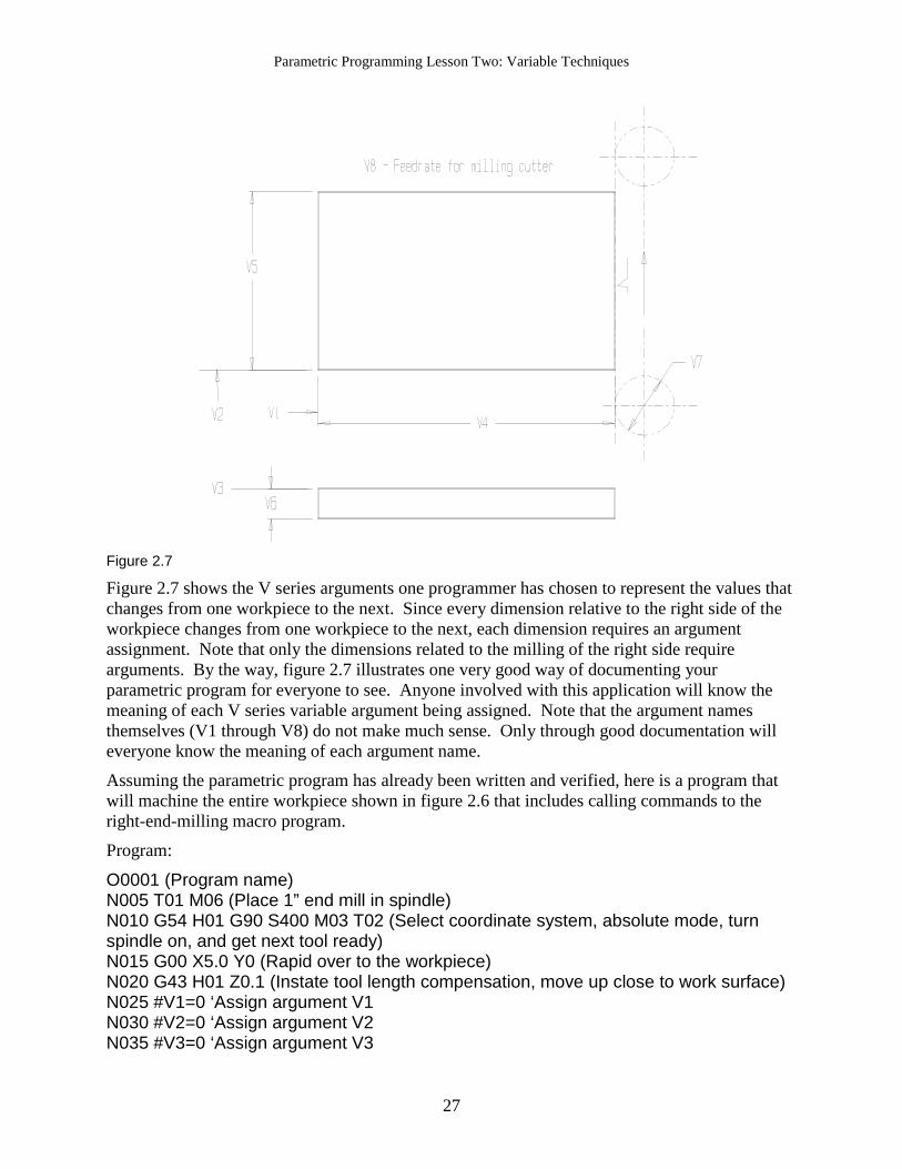
Figure 2.7 shows the V series arguments one programmer has chosen to represent the values that changes from one workpiece to the next. Since every dimension relative to the right side of the workpiece changes from one workpiece to the next, each dimension requires an argument assignment. Note that only the dimensions related to the milling of the right side require arguments. By the way, figure 2.7 illustrates one very good way of documenting your parametric program for everyone to see. Anyone involved with this application will know the meaning of each V series variable argument being assigned. Note that the argument names themselves (V1 through V8) do not make much sense. Only through good documentation will everyone know the meaning of each argument name.

Assuming the parametric program has already been written and verified, here is a program that will machine the entire workpiece shown in figure 2.6 that includes calling commands to the right-end-milling macro program.

Program:

O0001 (Program name) N005 T01 M06 (Place 1” end mill in spindle) N010 G54 H01 G90 S400 M03 T02 (Select coordinate system, absolute mode, turn spindle on, and get next tool ready) N015 G00 X5.0 Y0 (Rapid over to the workpiece) N020 G43 H01 Z0.1 (Instate tool length compensation, move up close to work surface) N025 #V1=0 ‘Assign argument V1 N030 #V2=0 ‘Assign argument V2 N035 #V3=0 ‘Assign argument V3


28

N040 #V4=5.0 ‘Assign argument V4 N045 #V5=3.0 ‘Assign argument V5 N050 #V6=0.5 ‘Assign argument V6 N055 #V7=1.0 ‘Assign argument V7 N060 #V8=5.0 ‘Assign argument V8 N065 M98 P1000 (Mill right side) N070 G91 G28 Z0 M19 (Move to tool change position, orient spindle) N075 M01 (Optional stop) N080 T02 M06 (Place 1/2 drill two in spindle) N085 G54 G90 S800 M03 T01 (Select coordinate system, absolute mode, start spindle, get tool number one ready) N090 G00 X0.5 Y0.5 (Rapid to first hole position) N095 G43 H02 Z0.1 (Instate tool length compensation, rapid up close to work surface) N100 G81 R0.1 Z-0.85 F4.0 (Drill first hole) N105 Y2.5 (Drill second hole) N110 X4.5 (Drill third hole) N115 Y0.5 (drill fourth hole) N120 G80 (Cancel cycle) N125 G91 G28 Z0 M19 (Return to tool change position, orient spindle) N130 M02 (End of program) Note how little of this program deals with the milling of the right side. The series of commands from N025 through N060 simply set the V series variable arguments. Line N065 calls the macro program. If more workpieces must be milled by this program, it is easy to simply specify more calling commands (after changing the related V series variable arguments) to the program named O1000. Note from this example that V series variables must be designated one per command. Though this may at first seem a little cumbersome, keep in mind that this requirement can actually be a benefit when it comes to multiple call statements. Only those V series variables that change must be specified from one call statement to the next.

Here is the macro program that actually mills the right side. Notice that each value needed within the CNC program must first be transferred to an R series variable. Also notice that each argument is referenced directly by the V series variable being set in the main program.

O1000 (Macro program to mill right side) N1 #R0=V1+V4+V7/2 `Calculate X position for cutter N2 #R1=V2-0.1-V7/2 `Calculate Y starting position N3 #R2=V3-V6-0.1 `Calculate work surface position in Z N4 #R3=V2+V5+0.1+V7/2 `Calculate Y ending position N5 #R4 = V8 `Transfer feedrate into R4 N6 #R5 = V3 + 0.1 `Calculate clearance position in Z N7 G00 X+R0 Y+R1 (Rapid to starting position) N8 G01 Z+R2 F50. (Fast feed to work surface) N9 Y+R3 F+R4 (Mill right side) N10 G00 Z+R5 (Rapid to above workpiece) N11 M99 (End of parametric program) While this macro program should be relatively easy to follow, there are a few points we wish to make about its structure. First of all, notice that calculations must be done in order to determine


29

the positions needed during the milling cutter’s motions. Calculations require macro commands (as opposed to CNC commands), and all macro commands must begin with the pound sign (lines N1 through N6).

Second, notice that values needed during CNC words must be first stored in R series variables before they can be referenced in CNC commands. Even the simple feedrate value that does not require a calculation (in line N5) must first be placed into an R series variable. This line is also considered a macro command (it must begin with a pound sign) since it references data stored in a V series variable.

Finally, notice that arithmetic calculations are being done within several commands. While these simple arithmetic functions should be quite understandable, we will discuss the arithmetic functions of macro 2 in detail later.

Running out of R series variables? Even with this rather simple example, you may have noticed that we used six of the ten available R series variables. You may be somewhat concerned that there will not be enough R series variables for more complicated applications. While this is an understandable concern, keep in mind that R series variables can be used over and over again, even within the same program. Once an R series variable’s value is no longer needed, it can be reassigned and reused. Consider this second version of the macro program that only requires two R series variables.

O1000 (Macro program to mill right side) N1 #R0=V1+V4+V7/2 ‘Calculate X position for cutter N2 #R1=V2-0.1-V7/2 ‘Calculate Y starting position N3 G00 X+R0 Y+R1 (Rapid to starting position) N4 #R0=V3-V6-0.1 ‘Calculate work surface position in Z N5 G01 Z+R0 F50. (Fast feed to work surface) N6 #R0=V2+V5+0.1+V7/2 ‘Calculate Y ending position N7 #R1=V8 ‘Transfer feedrate into R4 N8 Y+R0 F+R1 (Mill right side) N9 #R0 = V3 + 0.1 ‘Calculate clearance position in Z N10 G00 Z+R0 (Rapid to above workpiece) N11 M99 (End of parametric program) Notice that as soon as an R series variable is no longer needed, it is reassigned and reused. This dramatically minimizes the number of R series variables needed within your macro programs and also reinforces the reason why you should only use R series variables for the purpose of getting data into CNC words.

V series variables as arguments for family-of-parts applications While the M98 command and corresponding V series variable argument assignments is the best way to pass data to a user created canned cycle macro program, it is not always the most convenient way to get data into the macro program. When programming family-of-parts applications, the entire workpiece is being machined by the parametric program. In this case, it is usually more convenient to state the values of all V series variable arguments at the very beginning of the program rather than to call the macro program from another program.

We will again use the workpiece in figure 2.6 for the example program, but will change the criteria of the application. Instead of just milling the right side for a variety of different


30

workpieces, we’ll say the workpiece shown in figure 2.6 is but one of over 100 very similar workpieces. All workpieces have four 1/2” diameter holes drilled 0.5 in from each edge. This new criteria (machining the entire workpiece) changes the application from a user-created canned cycle application to a family-of-parts application. Again, figure 2.7 shows the V series variable arguments related to this application. Since the hole locations are always 1/2” in diameter and 0.5 in from the edges, no additional V series variable arguments are required. Here is the macro program that machines all workpieces in this part family.

Program:

O0002 (Program name) (Argument assignments) N005 #V1 = 0 `Left side position in X N010 #V2 = 0 `Lower side position in Y N015 #V3 = 0 `Top surface of workpiece in Z N020 #V4 = 5.0 `Length of workpiece in X N025 #V5 = 3.0 `Width of workpiece in Y N030 #V6 = 0.5 `Workpiece thickness N035 #V7 = 1.0 `Milling cutter diameter N040 #V8 = 5.0 `Feedrate of milling cutter in IPM (Machining portion of the program) N045 T01 M06 (Place 1” end mill in spindle) N050 #R0=3.82*80/V7 `Calculate spindle speed in RPM N055 G54 G90 S+R0 M03 T02 (Select coordinate system, absolute mode, turn spindle on, and get next tool ready) N060 #R0=V1+V4+V7/2 `Calculate X position for milling cutter N065 #R1=V2-0.1-V7/2 `Calculate starting position in Y N070 G00 X+R0 Y+R1 (Rapid over to the workpiece) N075 #R0=V3+0.1 `Calculate rapid approach position in Z N080 G43 H01 Z+R0 (Instate tool length compensation, move up close to work surface) N085 #R0=V3-V6-0.1 `Calculate work surface position in Z N090 G01 Z+R0 F50.0 (Fast feed past surface) N095 #R0=V2+V5+0.1+V7/2 `Calculate Y ending position N100 #R1=V8 `Transfer feedrate value to R1 N105 Y+R0 F+R1 (Mill right side) N110 #R0=V3+0.1 `Calculate clearance position in Z N115 G00 Z+R0 (Rapid to above top surface) N120 G91 G28 Z0 M19 (Move to tool change position, orient spindle) N125 M01 (Optional stop) N130 T02 M06 (Place 1/2 drill two in spindle) N135 G54 G90 S800 M03 T01 (Select coordinate system, absolute mode, start spindle, get tool number one ready) N140 #R0=V1+0.5 `Calculate first hole X position N145 #R1=V2+0.5 `Calculate first hole Y position N150 G00 X+R0 Y+R1 (Rapid to first hole position) N155 #R3=V3+0.1 `Calculate rapid plane for hole machining N160 G43 H02 Z+R3 (Instate tool length compensation, rapid up close to work surface) N165 #R0=V3-V6-0.18 `Calculate hole bottom position


31

N170 G81 R0+R3 Z+R0 F4.0 (Drill first hole) N175 #R0=V2+V5-0.5 `Calculate second hole Y position N180 Y+R0 (Drill second hole) N185 #R0=V1+V4-0.5 `Calculate third hole X position N190 X+R0 (Drill third hole) N195 #R0=V2+0.5 N200 Y+R0 (drill fourth hole) N205 G80 (Cancel cycle) N210 G91 G28 Z0 M19 (Return to tool change position, orient spindle) N215 M02 (End of program) Notice how well the V series variable arguments are documented at the beginning of this program. Since their names are not recognizable, the comments to the right of the apostrophe stress the meaning of each. An operator or setup person could confidently modify any one these arguments during setup for the next workpiece in the family to be machined.

Also notice that arguments are only required for those things that change from one workpiece in the family to the next. Any value that does not change (speed and feed for 1/2” drill, 0.5 inch hole position, 0.1” approach distance, etc.) is treated as a constant value. Constant values, of course, cannot be changed by simply manipulating argument values.

While this is a relatively simple family-of-parts application, it should nicely stress how local variable arguments can be introduced to family-of-parts parametric programs. It should also begin to show you some of the power you have available with parametric programming.

Please note the subtle distinction between argument assignment for user-created canned cycle applications and argument assignment for family-of-parts applications. With part families, the macro program is machining the entire workpiece, and assigning arguments in the main program is the most convenient method of argument assignment since only one program is required.

On the other hand, since user-created canned cycle applications always require a separate program to perform the canned-cycle-like operation, and since this program may be required several times even to machine one workpiece, arguments must be set in the main program. And it must be possible to manipulate the arguments from one execution of the parametric program to the next.

Getting input from the operator One unique function of Fadal’s macro it the ability to get operator input during the execution of the CNC program. In essence, your macro program can query the operator for arguments to be used in the macro program. While you should always test the input data for mistakes (we’ll show how later), this can make an effective way to get arguments assigned for family of parts applications.

Here is a modified version of the family-of-parts application to mill the right side of a workpiece and drill four holes (shown in figure 2.7). Notice the use of the PRINT and INPUT statements that gets data from the operator.

Program:

O0003 (Program name) (Argument assignments) N005 #PRINT “ENTER LEFT SIDE POSITION IN X”


32

N010 #INPUT V1 N015 #PRINT “ENTER THE LOWER SURFACE POSITION IN Y” N020 #INPUT V2 N025 #PRINT “ENTER TOP SURFACE POSITION IN Z” N030 #INPUT V3 N035 #PRINT “ENTER LENGTH OF WORKPIECE IN X” N040 #INPUT V4 N045 #PRINT “ENTER WIDTH OF WORKPIECE IN Y” N050 #INPUT V5 N055 #PRINT “ENTER WORKPIECE THICKNESS” N060 #INPUT V6 N065 #PRINT “ENTER MILLING CUTTER DIAMETER” N070 #INPUT V7 N075 #PRINT “ENTER MILLING FEEDRATE” N080 #INPUT V8 (Machining portion of the program) N085 T01 M06 (Place 1” end mill in spindle) N090 #R0=3.82*80/V7 `Calculate spindle speed in RPM N095 G54 G90 S+R0 M03 T02 (Select coordinate system, absolute mode, turn spindle on, and get next tool ready) N100 #R0=V1+V4+V7/2 `Calculate X position for milling cutter N105 #R1=V2=0.1-V7/2 `Calculate starting position in Y N110 G00 X+R0 Y+R1 (Rapid over to the workpiece) N115 #R0=V3+0.1 `Calculate rapid approach position in Z N120 G43 H01 Z+R0 (Instate tool length compensation, move up close to work surface) N125 #R0=V3-V6-0.1 `Calculate work surface position in Z N130 G01 Z+R0 F50.0 (Fast feed past surface) N135 #R0=V2+V5+0.1+V7/2 `Calculate Y ending position N140 #R1=V8 `Transfer feedrate value to R1 N145 Y+R0 F+R1 (Mill right side) N150 #R0=V3+0.1 `Calculate clearance position in Z N155 G00 Z+R0 (Rapid to above top surface) N160 G91 G28 Z0 M19 (Move to tool change position, orient spindle) N165 M01 (Optional stop) N170 T02 M06 (Place 1/2 drill two in spindle) N175 G54 G90 S800 M03 T01 (Select coordinate system, absolute mode, start spindle, get tool number one ready) N180 #R0=V1+0.5 `Calculate first hole X position N185 #R1=V2+0.5 `Calculate first hole Y position N190 G00 X+R0 Y+R1 (Rapid to first hole position) N195 #R3=V3+0.1 `Calculate rapid plane for hole machining N200 G43 H02 Z+R3 (Instate tool length compensation, rapid up close to work surface) N205 #R0=V3-V6-0.18 `Calculate hole bottom position N210 G81 R0+R3 Z+R0 F4.0 (Drill first hole) N215 #R0=V2+V5-0.5 `Calculate second hole Y position N220 Y+R0 (Drill second hole)


33

N225 #R0=V1+V4-0.5 `Calculate third hole X position N230 X+R0 (Drill third hole) N235 #R0=V2+0.5 N240 Y+R0 (drill fourth hole) N245 G80 (Cancel cycle) N250 G91 G28 Z0 M19 (Return to tool change position, orient spindle) N255 M02 (End of program) As stated, this program requires refinement. First of all, nothing guards against operator mistakes when inputting data. The control will execute the motions of this program regardless of input error, which could be disastrous. We will discuss how you can test for mistakes during argument assignment in chapter four. Second, note that with this version of the program, the PRINT and INPUT commands will be executed every time the program is run. Unless your operator is making only one workpiece, entering so much data for each workpiece will not be feasible. We will also show a way of handling this problem later in this text.

Using V series variables as counters Looping functions often require that variables change each time the loop is executed. Though loops have yet to be introduced, a V series variable will be used as the loop counter and for any other variable that must be initialized at the beginning of the loop and stepped each time through the loop.

Using V series variables as flags It is sometimes necessary to set a flag that tells the macro program how to behave. For example, you may wish to set up criteria in your right-side milling user task program that allows the milling cutter to either climb or conventional mill. A special flag will specify which milling method you wish to use. In essence, you are flagging the macro program as to how it should behave. Other examples of when flags are required (that we will discuss in greater detail during our discussion of conditional branching) include right hand versus left hand tooling, inch versus metric input, and whether or not coolant is to be used. While V series variables prior to the M98 calling command commonly set flags, the global nature of V series variables makes it possible to maintain the values of flags even among several programs.

Retaining data among several programs Many parametric programming applications require several programs that work together. The more complicated the application, the more likely it is that more than one program will be required. As with any complicated problem, it is often helpful to divide the parametric programming application into smaller and easier-to-handle segments. V series variables should be used for any data that must be shared among two or more programs (this kind of data is commonly called global data).

It may be helpful, for example, to have one macro program calculating speeds and feeds. Another may be setting up the tool station numbers. And yet another actually doing the machining. In this case, speed, feed, and tool station values must be available to the machining program. V series variables should be used to maintain the value of each feed, speed, and tool station number from one program to another.


34

Retaining data from one day to the next One example of when it is necessary to retain data from day to day is part counting. Say you wish to set up a part counter to let the machine run 750 workpieces and then halt the machine (this application is show in detail later in this text). As you begin running production, macro based part counter will begin counting workpieces.

It isn’t very likely that you will finish all 750 workpieces before the end of the day/shift. It will be more likely that it will take several days to complete the production run. In this case, you will need your part counting macro program to remember where it left off from day to day. If you store the current part count in a V series variable, the value of the variable will not be lost when the power is turned off. Like tool offsets, the V series variables are retained after power off, and are even available for modification through the display screen and keyboard.

Setting your own system constants Think of any constant hard-and-fixed value that you use throughout your CNC programming. The first one that may come to mind is your rapid approach and retract distance. When programming in the inch mode, for example, many programmers like to stay a constant 0.100 in away from the surface being approached before entering a cutting mode. When cutting is completed, many programmers feed the tool away from the workpiece by this same 0.100 in amount.


If instead, a V series variable is used in which to store the rapid approach and retract distance, and if this variable is referenced in every CNC program during every tool’s approach and retract movement, changing the approach/retract distance will be as simple as changing one V series variable. V series variables can even be entered and changed through the keyboard and display screen, just like tool offsets, making it very easy to change the rapid approach/retract distance.

Consider this program that drills a few holes and mills a slot. It assumes the rapid approach/retract distance is stored in V series variable V1.

O0003 (Program that allows easy approach/retract distance change) N005 T01 M06 (Place 1/2 drill in spindle) N010 G54 G90 S800 M03 T02 (Select coordinate system, absolute mode, turn spindle on, and get tool number two ready) N015 G00 X.5 Y.5 (Rapid to first hole location) N017 #R1 = V1 ‘Set Approach distance to R1 N020 G43 H01 Z+R1 (Instate tool length compensation, rapid up to workpiece) N025 G81 R0+R1 Z-.85 F3.5 (Drill first hole) N030 Y3.5 (Drill second hole) N035 X4.5 (Drill third hole) N040 Y.5 (Drill fourth hole) N045 G80 (Cancel cycle) N050 G91 G28 Z0 (Return to tool change position) N055 M01 (Optional stop)


35

N060 T02 M06 (Place 3/8 drill in spindle) N065 G54 G90 S950 M03 T03 (Select coordinate system, absolute mode turn spindle on and get tool three ready) N075 G00 X3.0 Y2.0 (Rapid to hole location) N080 G43 H01 Z+R1 (Instate tool length compensation, rapid to approach position) N085 G81 R0+R1 Z-.55 F3.5 (Drill hole) N090 G80 (Cancel cycle) N095 G91 G28 Z0 (Return to tool change position) N100 M01 (Optional stop) N105 T03 M06 (Place 1/4” endmill in spindle) N110 G54 G90 S1000 M03 T01 (Select coordinate system, absolute mode turn spindle on and get tool one ready) N113 #R2=0.1+V1 ‘Set R2 to Y approach position N115 G00 X3.75 Y-R2 (Rapid to slot approach position) N120 G43 H01 Z-0.125 (Instate tool length compensation, rapid to work surface) N123 #R2=4.125+V1 ‘Set R2 to Y plus side of slot N125 G01 Y+R2 F2.5 (Mill slot) N130 G00 Z+R1 (Rapid to above work surface) N135 G91 G28 Z0 (Return to tool change position) N140 M02 (End of program) Notice that any time a tool in this program approaches or retracts (lines N020, N025, N080, N085, N115, N125, and N130), the value requiring the proper approach distance stored in V1 is referenced. In lines N113 and N123, notice how the programmer can even perform a calculation that has the control figure out the correct approach/retract position based on the current value of common variable V1. With this program, changing the approach/retract distance will be as easy as changing variable V1.

System variables Many of the CNC related features of Fadal’s macro are handled with system variables. These variables have special names (chosen by Fadal) and allow access to many CNC functions including current machine position, offsets, alarm generation, and much more. These variables will be well covered in the future chapters.

Summary of macro variables As you have seen, there are three types of variables in macro. R series variables, which are used to get data into a form by which it can be used in a CNC word. V series variables, which can be used for a variety of purposes, including as arguments, to minimize redundant calculations, for general purpose calculations, and as counters. And system variables which allow access to many CNC related features of macro. While you should have a pretty good idea of what variables do, remember that all presentations to this point have been rather elementary. There are some advanced implications yet to be discussed. We will address these advanced implications in future chapters.

Date post:	27-Oct-2018
Category:	Documents
Upload:	lamhuong
View:	221 times
Download:	0 times

Variable Techniques - elearningzoom.com · three popular versions of parametric programming:...

Documents