Variance Risk Premia in Commodity Markets Marcel Prokopczuk ,‡ and Chardin Wese Simen January 14, 2013 Abstract In this paper, we study variance risk premia in commodity markets. Using synthetic variance swaps, we find significant variance risk premia in 18 out of 21 markets. Typically, variance risk premia are negative, time-varying and their magnitudes increase with variance. Consistent with theory, we find a significant relation between variance risk premia and macroeconomic factors. Furthermore, we evaluate the information content of commodity variance risk premia for future returns. We show that gold’s variance risk premium has predictive power for returns in most of the markets considered. This economically significant predictive power is robust to the inclusion of traditional predictors. JEL classification: G12, G13 Keywords: Commodities, Variance risk premia, Variance swaps Marcel Prokopczuk gratefully acknowledges financial support from the British Academy. We thank Lazaros Symeonidis for helpful comments. Contact: [email protected] (M. Prokopczuk) and [email protected] (C. Wese Simen). Chair of Empirical Finance and Econometrics, Zeppelin University, 88045 Friedrichshafen, Germany. ICMA Centre, Henley Business School, University of Reading, Reading, RG6 6BA, United Kingdom.
Transcript
Variance Risk Premia in Commodity
Markets*Marcel Prokopczuk�,‡ and Chardin Wese Simen�
January 14, 2013
Abstract
In this paper, we study variance risk premia in commodity markets. Using
synthetic variance swaps, we find significant variance risk premia in 18 out
of 21 markets. Typically, variance risk premia are negative, time-varying
and their magnitudes increase with variance. Consistent with theory, we
find a significant relation between variance risk premia and macroeconomic
factors. Furthermore, we evaluate the information content of commodity
variance risk premia for future returns. We show that gold’s variance risk
premium has predictive power for returns in most of the markets considered.
This economically significant predictive power is robust to the inclusion of
traditional predictors.
JEL classification: G12, G13
Keywords: Commodities, Variance risk premia, Variance swaps*Marcel Prokopczuk gratefully acknowledges financial support from the British Academy.We thank Lazaros Symeonidis for helpful comments. Contact: [email protected] (M.Prokopczuk) and [email protected] (C. Wese Simen).�Chair of Empirical Finance and Econometrics, Zeppelin University, 88045 Friedrichshafen,Germany.�ICMA Centre, Henley Business School, University of Reading, Reading, RG6 6BA, UnitedKingdom.
I Introduction
Over the past decade, commodity markets have not only witnessed substantial
growth but also tremendous increases in prices and volatility. Given their role as
consumption goods, factors of production and financial assets, managing commodity
price volatility is crucial for a wide number of market participants such as commercial
hedgers and investors. Arguably, these developments have motivated the successful
launch of commodity related volatility derivatives such as oil and gold VIX futures
contracts. The rapid proliferation of these derivatives raises several questions. Chief
among them include: how large is the compensation required by investors to bear
variance risk in commodity markets? To what degree are commodity variance
risk premia time-varying? What are the determinants of variance risk premia in
commodity markets? In this paper we seek to answer these questions.
We study variance risk premia in 21 commodity markets between 1989 and 2011,
a period which includes the run-up to the recent financial crisis. In doing so, we
contribute to the literature in at least three ways. To start with, we are, to the best
of our knowledge, the first to comprehensively examine the extent to which variance
risk is priced in a wide variety of commodity markets. Our large data set enables
us to investigate variance risk premia in diverse commodities including the grains,
energy and metals markets. Additionally, by analyzing variance swaps of different
maturities, we shed some light on the shape and behavior of the term-structure of
variance risk premia.
Second, we thoroughly investigate the determinants of commodity variance
risk premia. In particular, we examine the link between commodity variables,
macroeconomic factors and variance risk premia. Moreover, the different
volatility behaviors of commodities highlighted by Brooks and Prokopczuk (2011)
1
make commodity markets well-suited to clearly distinguish between two popular
rationalizations of the sign of variance risk premia: the diversification benefit and
the insurance premia hypotheses.
Third, we evaluate the predictive power of commodity variance risk premia for
returns across multiple horizons and markets. Here, our focus differs from existing
studies in that we also investigate whether a commodity’s variance risk premium
predicts not only its own returns but also those of other commodities.
Our main findings can be summarized as follows. Variance risk is significantly
priced in 18 out of 21 commodity markets. Generally, the evidence points to negative
variance risk premia with magnitudes rising in variance levels. These findings hold
for different maturities and also over the recent financial crisis. Furthermore, our
results support the insurance premia hypothesis, implying a strong link between
macroeconomic factors and variance risk premia. Consistent with the predictions of
Bakshi and Madan (2006), we find that individual macroeconomic factors explain
as much as 20.4% of movements in variance risk premia. Commodity specific
factors can help too: the basis, hedging pressure and open interest complement
the explanatory power of macroeconomic factors by 34% on average. Finally, we
demonstrate that gold’s variance risk premium predicts returns with significantly
negative coefficients for as many as 13 markets. Typically, the predictive power
manifests itself at all horizons and is robust to the inclusion of traditional predictors
such as the basis and open interest.
Most existing papers studying variance risk premia focus on the question of
whether variance risk is priced in equity markets. Applying hedging-based tests,
Bakshi and Kapadia (2003b) and Coval and Shumway (2001) present evidence of
priced volatility risk in equity indices. Hafner and Wallmeier (2007), Carr and Wu
2
(2009) and Driessen et al. (2009) implement a model-free approach and document
negative variance risk premia in leading European and US stock indices. In contrast,
the evidence for individual stocks is somewhat mixed. While Carr and Wu (2009)
report significantly negative variance risk premia in 8 out of 35 individual equities
only, Driessen et al. (2009) find marginally positive variance risk premia for some
stocks.
Some studies investigate the market price of variance risk in other traditional
asset classes. Estimating the Heston (1993) model for the Dollar/Mark market,
Guo (1998) reports that, between 1987 and 1992, the market price of variance risk
ranges from −4.1 to 1.3. Low and Zhang (2005) reach similar conclusions for other
currencies. They show that investors writing straddles earn as much as 2.4% per
annum in the British Pound market and conclude that volatility risk is negatively
priced in currency markets during the period 1996–2003. Additionally, their evidence
suggests that the performance of this strategy decreases as the horizon increases.
Similarly, Simon (2010) finds that short straddles in fixed-income markets are highly
profitable. Mueller et al. (2011) synthesize variance swaps and provide evidence of
negative variance risk premia in the US Treasury bond market.
In contrast to traditional asset classes, the literature on variance risk premia
in commodity markets is somewhat scant.1 Employing relatively simple parametric
models, Doran and Ronn (2008) estimate variance risk premia of −0.9, −0.4 and
−1.4 for crude oil, heating oil and natural gas, respectively. Similarly, Trolle and
Schwartz (2010) show that long variance swap positions lose 2.96% and 3.58% on
average in the crude oil and natural gas markets, respectively. In a related study,
1Similar observations can be made for other emerging asset classes such as credit and volatility.Wang et al. (2010) and Barnea and Hogan (2012) are the only studies on variance risk premia inthe credit default swap (CDS) and VIX markets we are aware of.
3
Wang et al. (2011) find that corn variance swaps are unprofitable, indicating a
negative price of variance risk for corn.
Overall, existing studies unanimously point to negative variance risk premia
in financial markets, which contrasts with the positive compensation required
by investors for price risk. This seemingly counterintuitive result raises several
questions: why do investors pay a premium for taking on variance risk? What are
the determinants of variance risk premia?
The literature proposes two main hypotheses: the diversification benefit and the
insurance premia against bad economic states. On the one hand, the diversification
benefit hypothesis argues that the sign of variance risk premia is determined by the
correlation between returns and volatility. Specifically, if returns and volatility are
negatively correlated as is the case for equities, variance swaps provide good hedges
for price risk. Investors are willing to pay a variance risk premium to obtain this
diversification benefit. Conversely, if returns and volatility are positively correlated,
it is plausible that investors will require a compensation for bearing this extra risk.
On the other hand, the insurance premia hypothesis links with the insights
of Bakshi and Madan (2006), who argue that volatility risk premia arise because
“rational risk-averse investors are sensitive to extreme loss states and are willing
to counteract these exposures by buying protection”. This statement assimilates
variance risk premia to insurance premia against bad states of the economy.
Drechsler and Yaron (2011) formalize this intuition by developing an equilibrium
model in which investors are not only averse to uncertainty but also have a preference
for early uncertainty resolution. Their intuition is simple: if investors dislike
increases in economic uncertainty, they will pay a premium to hedge variance risk.
Drechsler (2012) and Mueller et al. (2011) provide empirical evidence in support
4
of this conjecture. It is important to note that, unlike the diversification benefit
argument, this hypothesis always predicts a negative price of variance risk.
Another strand of the literature explores the information content of variance
risk premia for future returns. Bollerslev et al. (2009) show that, between 1990 and
2007, the S&P 500 variance risk premium accounts for as much as 7% of variations
in its returns. Using a more recent sample (2000–2011), Bollerslev et al. (2011b)
confirm this finding: the S&P 500 variance risk premium explains 13.02% of changes
in quarterly returns. Moreover, the authors document analogous predictive patterns
for major international stock markets.
Although the above studies significantly enhance our understanding of variance
risk premia, they suffer from several limitations. First, commodity related studies
are limited in scope. Together, Trolle and Schwartz (2010) and Wang et al. (2011)
merely cover 3 markets. In light of the mixed evidence for equities, it may be
that their findings are market specific: thus the necessity to study variance risk
premia in a large number of commodity markets. Second, because of their relatively
short and uneventful sample period, existing studies do not shed light on the
dynamics of variance risk premia during the recent boom in commodity prices or
the run-up to the recent financial crisis. Third, most studies invariably focus on
one horizon, overlooking crucial information in the term-structure of variance risk
premia. Examining variance risk premia across different maturities could provide
insights into the term-structure of variance risk premia. Fourth, to date, no empirical
study has ascertained which of the two hypotheses put forward to explain the sign
of variance risk premia is more likely. Indeed, the negative correlation between
price and volatility that prevails in traditional markets makes it difficult to clearly
distinguish between the two conjectures. Brooks and Prokopczuk (2011) show that
5
commodities such as gold and silver exhibit a positive price/volatility correlation,
making commodity markets a perfect testing ground to distinguish between the
two hypotheses. Fifth, the literature has only considered systematic factors in
its analysis of the determinants of variance risk premia. Despite the empirical
evidence of Mueller et al. (2011), it is possible that market specific conditions such
as inventories and open interest affect variance risk premia. Sixth, we examine
whether the predictive power of variance risk premia for future returns is validated in
commodity markets. More important, we assess whether a commodity variance risk
premium contains information not only for its returns but also for other commodity
returns.
This paper proceeds as follows. In Section II we introduce our methodology and
describe the data set employed. In Section III we present and discuss the empirical
results of our study. Finally, Section IV concludes.
II Methodology and Data
A. Methodology
Empirical studies on variance risk premia are usually anchored around one of the
following three estimation approaches: parametric, semi-parametric or model-free.
The parametric approach consists of specifying a data-generating process for
the underlying. In this framework, the variance risk premium is usually a
parameter to be estimated by exploiting information from the underlying and options
prices. This approach is not only computationally intensive but also subject to
specification errors since it explicitly assumes a specific data-generating process
for the underlying. Consequently, parametric estimates of variance risk premia
6
are joint tests of model specification and variance risk premia. Broadie et al.
(2007) empirically examine the impact of model misspecification on risk premia.
They conclude that the significance of variance risk premia depends crucially on
assumptions about the presence of jumps in the data-generating process.2
Bakshi and Kapadia (2003a) propose to study variance risk premia in a semi-
parametric way through option hedging errors by analyzing the profitability of delta-
hedged at-the-money (ATM) straddles. This approach is motivated by financial
theory, which argues that option prices are affected by changes in implied volatility
and the underlying’s price. Since delta-neutral ATM straddles are insensitive to
small movements of the underlying’s price, their profitability is mainly driven by
changes in implied volatility. Hence, the profitability of delta-neutral ATM straddles
may shed light on the existence of variance risk premia. Though intuitive, this
approach is subject to the criticism that it does not allow for jump risk. Given the
evidence discussed by Eraker et al. (2003) and Pan (2002), this omission is likely
to be a serious issue. Echoing this concern, Branger and Schlag (2008) warn that
hedging-based tests may mistakenly attribute the combined effect of volatility and
jump risk premia to volatility risk premia, potentially leading to wrong inferences
on the sign, significance and size of volatility risk premia.
To overcome these problems, the more recently introduced model-free approach
builds on variance swaps defined as swap contracts in which the floating leg
corresponds to the realized variance of the underlying over a predetermined period.
The underlying idea is that variance risk premia are equal to the pay-offs of variance
swaps which are the differences between the realized variance and the risk-neutral
expectation of variance. No-arbitrage arguments imply that the rate of a variance
2Pan (2002) reaches similar conclusions. She shows that once jumps are allowed for, thevariance risk premium becomes insignificant in her data set.
7
swap, SVt,T , must be equal to the risk-neutral expectation of variance EQt (Vt,T ) over
the life of the swap. Thus, the variance risk premium at date t and horizon T ,
V RPt,T , is given by:
V RPt,T = RVt,T − SVt,T (1)
where RV (t, T ) denotes the realized variance between t and T under the physical
measure.3
Consequently, quantifying variance risk premia reduces to estimating realized
variance and variance swap rates. Whilst realized variance estimators have been
extensively studied (see, e.g., Andersen et al. (2009) and the references therein), until
recently, little has been known about the latter. In a seminal study, Britten-Jones
and Neuberger (2000) elaborate a replicating strategy to estimate the variance swap
rate under the assumption that the underlying follows a continuous process.4 More
precisely, they derive the following estimator:
EQt (Vt,T ) = MFIVt,T =
2ert(T−t)
T − t
[∫ F
0
P (K)
K2dK +
∫ +∞
F
C(K)
K2dK
]
(2)
where EQt (Vt,T ) and MFIVt,T refer to the risk-neutral expectation of variance and
model-free implied variance between t and T , respectively. The annualized risk-free
rate is denoted by rt, and P (K) and C(K) denote European put and call options
struck at K.
Subsequently, Jiang and Tian (2005) extend this approach to a broader class
of models by formally showing that Equation (2) holds for jump diffusion models
3This implicitly assumes, of course, that the expectation of realized variance under the physicalmeasure is an unbiased estimate of realized variance.
4See Demeterfi et al. (1999) for an excellent treatment of the replicating strategy.
8
also. Although jumps introduce errors in the replicating strategy, the numerical
analysis of Carr and Wu (2009) indicates that these biases are negligible. Together,
these results lead to the conclusion that the variance swap approach for estimating
variance risk premia is robust and, more importantly, model-free in the sense that
it does not require assumptions about the underlying data-generating process.
Therefore, we employ a methodology that is similar to that of Carr and Wu
(2009). Assume we want to synthetically create a 60 day variance swap. On each
trading day, we obtain and sort all out-of-the-money (OTM) options by time to
maturity. We identify the two maturities T1 and T2 that are closest to and cover 60
days. We retain options of maturities T1 and T2 only. As in Trolle and Schwartz
(2010), we truncate the first and second integrals in Equation (2) at Kl and Ku
respectively:
Kl = St exp−10σT (3)
Ku = St exp10σT (4)
where Kl and Ku refer to the lower and higher truncated strikes. St refers to the
underlying price on day t, σ is the average implied volatility of all OTM options and
T denotes the time to maturity of the synthetic variance swap. For each maturity,
we linearly interpolate available implied volatilities across moneyness.5 For strikes
higher (lower) than the highest (lowest) listed strike price but lower (higher) than
Ku (Kl), we assume constant implied volatility. Pursuing this approach, we obtain
a grid of 1,000 equidistant implied volatilities for strikes between Ku and Kl. To
ensure that our interpolated implied volatilities are realistic, we require the existence
of at least two OTM put and two OTM call options for each of the two maturities.
5We obtain similar results with a spline interpolation. These results are available upon request.
9
We exclude from our sample all trading days that do not meet this requirement.
We then convert implied volatilities into European option prices using the Black
(1976) option pricing formula. We evaluate the integrands at each of the 1,000
points and numerically approximate (trapezoidal rule) the integrals in Equation (2)
to estimate the variance swap rate. Finally, we linearly interpolate between the two
swap rates to obtain the 60 day variance swap rate. We repeat the above steps every
day to obtain time series of 60 day variance swap rates.
As is common in empirical studies, we estimate realized variance as follows:
RVt,t+N =252
N
t+N∑
i=t+1
(
logFi,t+N
Fi−1,t+N
)2
(5)
where N is the time to maturity of the variance swap, Fi,t+N denotes the futures
contract observed at time i and expiring at time t+N .
Note that, contrary to individual equities, commodity options are written on
futures contracts which life span is finite. As a result, the time series of the
first nearby contract could exhibit spikes at rollover dates especially in markets
characterized by steep term-structure of futures. Given that these spikes could bias
our estimates of realized variance upward, we construct a constant maturity futures
time series by linear interpolation of futures contracts maturing at T1 and T2.
B. Data
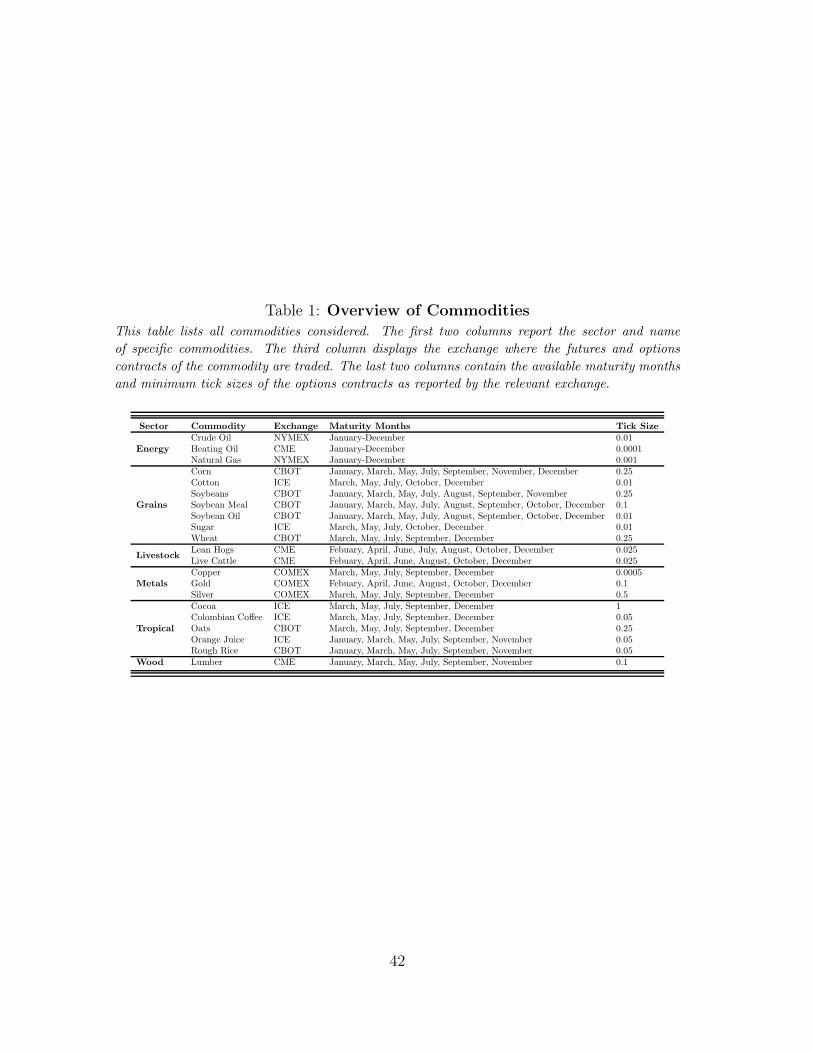
We obtain futures and option settlement prices from the Commodity Research
Bureau (CRB). Table 1 lists the 21 commodities included in our sample. To mitigate
the effect of micro-structure related issues such as infrequent trading and stale prices,
we only retain options with time-to-maturity of at least 12 days. We further delete
10
options with prices lower than five times the minimum tick size reported in the last
column of Table 1. Given that our data set comprises American options and that our
estimation approach requires European option prices, we follow Trolle and Schwartz
(2009) and convert the American options prices into European prices employing the
approximation of Barone-Adesi and Whaley (1987).
In light of our focus on variance swaps that mature in 60 or 90 days, we retain
only OTM options on the first two futures contracts. For energy commodities, we
retain OTM options on the second and third futures contracts.6 Table 2 gives an
overview of the final data set of option prices. It shows that our sample period spans
more than 20 years including the recent financial crisis. The last two columns report
the average number of OTM call and put options per trading day. These numbers
vary a lot across commodities. In particular, the number of OTM options for energy
commodities is substantially higher than for the other sectors. On average across all
commodities, there are 17 and 14 OTM call and put options per day, respectively.
III Empirical Results
Prior to discussing our empirical results, it is instructive to visually examine
the dynamics of realized variance (RV) and model-free implied variance (MFIV).
Figure 1 plots the time series of RV and MFIV for 6 commodities drawn from
different sectors. This figure highlights several interesting features. First, RV
and MFIV trend together. Second, MFIV is usually higher than RV, suggesting
that long variance swaps investments are generally unprofitable. However, by
visually inspecting these plots, it is impossible to ascertain whether these losses
6The reason for selecting the second and third nearby futures contracts is that, unlike othercommodities, energy commodities have a monthly expiration schedule.
11
are significantly different from zero or whether similar results are obtained for other
commodities. Third, the top right panel (soybean) reveals seasonal patterns in the
two estimates of variance, raising questions as to whether variance risk premia are
seasonal? Fourth, the scales of the vertical axes indicate that some commodities are
more volatile than others, prompting us to explore the connection between variance
risk premia and variance level. Finally, the figure shows that the two variance
estimates exhibit considerable temporal variations, leading us to analyze the drivers
of variance risk premia. We elaborate on each of the above observations in the
ensuing paragraphs.
A. Is Variance Risk Priced in Commodity Markets?
We start our empirical analysis by ascertaining whether variance risk is priced in
commodity markets. If variance risk is not priced, we expect one or a combination
of the following scenarios. First, the average pay-off to variance swaps is of small
magnitude, a few basis points at best. Second, the average pay-off is not statistically
distinguishable from zero.
A.1 Evidence of Variance Risk Premia
Table 3 presents summary statistics of the estimated commodity variance risk
premia. The average 60 day variance risk premia reported in Panel A ranges from
−10.2% (natural gas) to 2.6% (cotton), suggesting that variance risk is priced in
commodity markets and also that the market price of variance risk exhibits large
cross-sectional variations. To assess the significance of variance risk premia, we
report Newey-West t-statistics in the fourth column of Table 3. The evidence for 60
day variance risk premia (Panel A) suggests that variance swaps generate significant
12
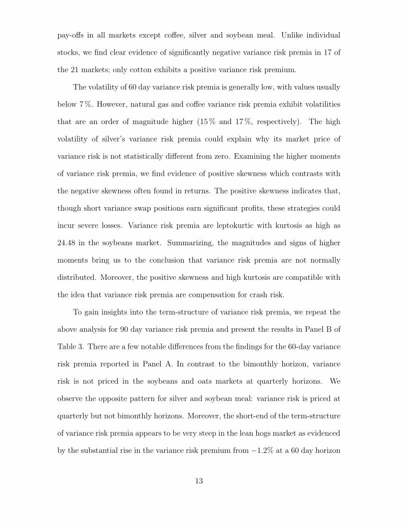
pay-offs in all markets except coffee, silver and soybean meal. Unlike individual
stocks, we find clear evidence of significantly negative variance risk premia in 17 of
the 21 markets; only cotton exhibits a positive variance risk premium.
The volatility of 60 day variance risk premia is generally low, with values usually
below 7%. However, natural gas and coffee variance risk premia exhibit volatilities
that are an order of magnitude higher (15% and 17%, respectively). The high
volatility of silver’s variance risk premia could explain why its market price of
variance risk is not statistically different from zero. Examining the higher moments
of variance risk premia, we find evidence of positive skewness which contrasts with
the negative skewness often found in returns. The positive skewness indicates that,
though short variance swap positions earn significant profits, these strategies could
incur severe losses. Variance risk premia are leptokurtic with kurtosis as high as
24.48 in the soybeans market. Summarizing, the magnitudes and signs of higher
moments bring us to the conclusion that variance risk premia are not normally
distributed. Moreover, the positive skewness and high kurtosis are compatible with
the idea that variance risk premia are compensation for crash risk.
To gain insights into the term-structure of variance risk premia, we repeat the
above analysis for 90 day variance risk premia and present the results in Panel B of
Table 3. There are a few notable differences from the findings for the 60-day variance
risk premia reported in Panel A. In contrast to the bimonthly horizon, variance
risk is not priced in the soybeans and oats markets at quarterly horizons. We
observe the opposite pattern for silver and soybean meal: variance risk is priced at
quarterly but not bimonthly horizons. Moreover, the short-end of the term-structure
of variance risk premia appears to be very steep in the lean hogs market as evidenced
by the substantial rise in the variance risk premium from −1.2% at a 60 day horizon
13
to 4.3%.7 Together, these results highlight important differences in the pricing of
variance risk across maturities.
In summary, Table 3 unequivocally points to significant variance risk premia in
commodity markets. Our conclusions tie in with previous work. By showing that
variance risk is negatively priced in energy markets, we extend the findings of Trolle
and Schwartz (2010) to longer horizons (60 and 90 days). Similarly, our results
for corn (90 day) corroborate and supplement the evidence of Wang et al. (2011).
However, our evidence of significant variance risk premia for most commodities
differs from that of individual equities reported in Carr and Wu (2009) and Driessen
et al. (2009). This result underscores the differences across asset classes.
Moreover, Table 3 has a more profound implication in that it provides
evidence against the diversification benefit hypothesis. As previously discussed,
this hypothesis posits that the sign of variance risk premia is determined by the
price/volatility correlation of the underlying asset. Given the findings of Brooks
and Prokopczuk (2011) that several commodities, such as gold, silver and soybeans,
exhibit positive price/volatility correlation, we would expect a positive variance
risk premium in these 3 markets. Table 3 rejects this hypothesis. In contrast, it
documents significantly negative premia for gold, silver and soybeans (for soybeans
only the 90 day premium is insignificant). Moreover, the evidence points to negative
variance risk premia in most markets at either 2 or 3 month horizons. We interpret
these results as empirical evidence against the diversification benefit hypothesis.
We formally explore the insurance premium hypothesis which links macroeconomic
expectations, uncertainty and variance risk premia in Subsection C.
7Further analysis reveals that the difference between the two premia is essentially driven byrealized variance.
14
A.2 Cross-market Comparisons
The highly negative variance risk premia of natural gas (at both maturities)
potentially indicates that more volatile commodities exhibit higher variance risk
premia. If confirmed, this feature could complicate cross-market comparisons. To
control for the overall volatility level, we compute the Log Variance Risk Premium
(LVRP) defined as LV RPt,T = log[
RVt,T
MFIVt,T
]
. An alternative approach consists
in calculating changes in daily variance risk premia. However, we favour LVRP
because it can be interpreted as the return of a variance swap. Moreover, LVRP are
conducive to cross-market comparisons since traditional performance measures such
as Sharpe ratios (SR) can be computed for returns series.
Table 4 displays the results of the analysis for the LVRP. Again, we report
results for 60 and 90 day variance swaps in Panels A and B, respectively. The mean
LVRPs reported in Panel A of Table 4 range from−86.5% (oats) to 66.9% (cotton).8
The standard deviation of the LVRP is fairly homogenous across commodities with
values typically below 50%, the only exception being silver with a high volatility
of 121%. The relatively low higher moments indicate that LVRPs are better
approximated by a Gaussian distribution than variance risk premia.
To evaluate the performance of commodity variance swaps, we report absolute
values of annualized, Newey-West corrected SRs in the penultimate column of Table
4. We present absolute values of SR because the negative returns on variance swaps
complicate cross-market comparisons of SRs. Koijen et al. (2012) show that long
passive commodity investments earn SRs of about 10% for the period 1980–2011.
Table 4 demonstrates that 60 day commodity variance swaps outperform long passive
strategies with SRs varying between 9.4% and 63.4%. The high variability in
8Note that under the null of no variance risk premium, LVRP will be negative due to Jensen’sinequality.
15
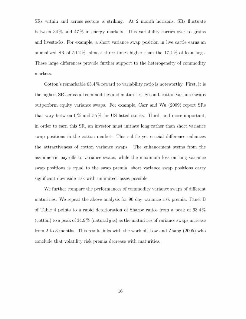
SRs within and across sectors is striking. At 2 month horizons, SRs fluctuate
between 34% and 47% in energy markets. This variability carries over to grains
and livestocks. For example, a short variance swap position in live cattle earns an
annualized SR of 50.2%, almost three times higher than the 17.4% of lean hogs.
These large differences provide further support to the heterogeneity of commodity
markets.
Cotton’s remarkable 63.4% reward to variability ratio is noteworthy. First, it is
the highest SR across all commodities and maturities. Second, cotton variance swaps
outperform equity variance swaps. For example, Carr and Wu (2009) report SRs
that vary between 0% and 55% for US listed stocks. Third, and more important,
in order to earn this SR, an investor must initiate long rather than short variance
swap positions in the cotton market. This subtle yet crucial difference enhances
the attractiveness of cotton variance swaps. The enhancement stems from the
asymmetric pay-offs to variance swaps; while the maximum loss on long variance
swap positions is equal to the swap premia, short variance swap positions carry
significant downside risk with unlimited losses possible.
We further compare the performances of commodity variance swaps of different
maturities. We repeat the above analysis for 90 day variance risk premia. Panel B
of Table 4 points to a rapid deterioration of Sharpe ratios from a peak of 63.4%
(cotton) to a peak of 34.9% (natural gas) as the maturities of variance swaps increase
from 2 to 3 months. This result links with the work of, Low and Zhang (2005) who
conclude that volatility risk premia decrease with maturities.
16
B. Time Variation in Variance Risk Premia
In the following paragraphs, we analyze time variations in variance risk premia.
First, we examine seasonal patterns in variance risk premia. Second, we study the
link between variance and variance risk premia.
B.1 Affine Premium
It is possible that the large cross-sectional variations in variance risk premia reported
in Table 3 are the results of a negative relationship between variance risk premia and
variances. In fact, several stochastic volatility models (e.g. Heston (1993)) specify
the variance risk premium as an affine function of volatility. We formally test this
possibility by regressing realized variance on model-free implied variance:
RVt,T = α + βMFIVt,T + ε. (6)
The null hypothesis is that of a one-to-one relationship between realized and model-
free implied variance, i.e. the slope coefficient is not significantly different from
1.
The first five columns of Table 5 report the results from Regression (6). Starting
with 60 day variance risk premia, we find that, except for soybeans and soybean
meal, the slope estimates are always significantly lower than 1. In line with our
conjecture, this result confirms a negative relationship between V RP and MFIV .
We also assess whether relative variance risk premia are time-varying by estimating
the following regression:
log(RVt,T ) = α + β log(MFIVt,T ) + ε. (7)
17
In the last five columns of Panel A, we report the coefficients, t-statistics and
R2 of the above regression. The main findings do not change. We cannot reject the
null hypothesis at the 5% level for corn and soybeans only.
Panel B of Table 5 presents our findings for variance swaps that mature in 3
months. There are a few minor differences compared to Panel A. For example, we
cannot reject the null hypothesis (β = 1) for cotton, soybeans, soybean meal, wheat,
lean hogs and oats. Nevertheless, our main conclusion is unaltered: the profitability
of short variance swaps positions increases with variance.
Contrary to Trolle and Schwartz (2010), we find that natural gas LVRP
decreases with variance. The divergence of results is most likely due to our different
sample period and horizon. In addition, our evidence for commodity LVRP differs
from that of Carr and Wu (2009), who find that log variance risk premia are
independent of log realized variance in equity markets.
B.2 Calendar Effects
Many commodities exhibit seasonal patterns. Suenaga et al. (2008) document the
seasonality of realized variance in the natural gas market whereas Back et al. (2013)
document seasonality in implied volatilities. A priori, it is not clear whether this
pattern carries through to variance risk premia. On the one hand, if MFIV is a
forward looking measure of realized variance, it should capture the seasonal pattern
and therefore both, RV and MFIV vary with the seasonal cycle. This reasoning is
borne out by the plots of RV and MFIV for soybeans (Figure 1). Following this
argument, it is possible that variance risk premia do not exhibit any seasonality.
On the other hand, if the market price of variance risk is equivalent to an insurance
risk premium, its magnitude may be seasonal, varying with market related factors
18
such as crop cycles and weather conditions. Hence, we can reasonably expect sizable
variance risk premia at times when commodities are most sensitive to demand and/or
supply factors.
In order to establish which of the two conjectures applies, we compute monthly
averages of variance risk premia which we report in Table 6.9 In most markets, the
signs of variance risk premia are remarkably stable across months. However, the
month-by-month analysis also highlights large fluctuations in the magnitude and
significance of variance risk premia. In line with Trolle and Schwartz (2010), we
uncover economically large differences in natural gas’s variance risk premium. In
particular, the variance risk premium is considerably higher during the period July–
January than the period February–June. Further statistical tests indicate that the
difference between the 60 day variance risk premia of March (−4.3%) and September
(20.5%) is significant at the 5% level. Together, these findings provide evidence of
time regularities in the market price of natural gas’s variance risk. Orange juice is
another interesting case: its variance risk premium is significant in October–January
and July only. Economically, these months coincide with periods when orange juice
crops are most vulnerable to weather conditions. Notice also that results for soybean
meal and coffee indicate that variance risk is priced for a few months only. However,
the unconditional results reported in Table 3 do not provide evidence of significant
variance risk premia. Together, these results show that there is significant scope for
timing commodity variance swaps investments.
In summary, we document important time variations in commodity variance
risk premia. This finding is of great interest for academics and investors alike.
9For brevity, we report and discuss only the results pertaining to bimonthly variance riskpremia. Results for variance swaps that mature in 90 days are similar and are available uponrequest.
19
First, we demonstrate the importance of timing commodity variance swaps (e.g.
natural gas, orange juice, soybean meal). Second, our results are important for
commodity pricing. For example, the finding that orange juice’s variance risk
premium is only significantly negative when crops are most vulnerable to weather
conditions, indicates that commodity specific factors such as inventories and weather
may play an important role in enhancing our understanding of variance risk premia,
as it is likely that variance risk premia are not only affected by systematic but also
commodity specific factors.
C. Determinants of Variance Risk Premia
Having documented the existence of time-varying variance risk premia, we now turn
to the question of identifying the determinants of commodity variance risk premia.
C.1 Macroeconomic Expectations
Bollerslev et al. (2011a) relate variance risk premia to time-varying risk aversion,
suggesting that variations in variance risk premia may be attributable to the state
of the economy. Motivated by this insight, we investigate whether macroeconomic
expectations can account for variations in variance risk premia.
We proxy time-varying risk aversion with 2 financial variables: the default
spread (DFSPD) defined as the difference between AAA and BAA and the term
spread (TSPD) calculated as the difference between 10 year and 2 year bond
yields. We download these data from the Federal Reserve website. Additionally,
expectations of macroeconomic activity are obtained from Blue Chip Economic
Indicators (BCEI). This data set presents three distinct advantages over traditional
data sources of economic expectations such as the Survey of Professional Forecasters
20
(SPF) and the Livingstone Survey. First, BCEI surveys more than 40 experts
from leading academic institutions, banks, consultancies and insurers. Moreover,
respondents provide forecasts for several variables, ranging from GDP to net exports.
Second, these surveys are conducted at a monthly frequency. By contrast, the
SPF and the Livingston Survey are only available at quarterly and semi-annual
frequencies, respectively. Third, BCEI presents forecasts for the current and
following calendar years, making this data set well-suited for studies on long-run
uncertainty.10
To obtain consensus expectations for each month, we obtain individual
forecasts of different variables closely linked to economic activity and compute the
cross-sectional median.11 More precisely, we obtain consensus forecasts for real
gross domestic production (RGDP), the consumer price index (CPI) and industrial
production (IP). Each of these variables reveals information about different facets
of the economy. For example, RGDP and CPI are informative about the real and
nominal economy, respectively. Similarly, industrial production is closely linked to
commodity demand.
If variance risk premia are interpreted as insurance premia, positive macroe-
conomic expectations will translate into less negative variance risk premia. As a
result, RGDP and IP should be positively related with variance risk premia in
all commodity markets where they are negative. Table 7 summarizes the results of
regressions of variance risk premia on each macroeconomic forecast.12 In the interest
10Unfortunately the BCEI surveys are only available in PDF format. Therefore, we manuallyextracted and digitized the data.
11Note that the fixed forecasting horizon introduces some seasonality in individual series. Forexample, in January 2004, the current year forecast refers to the period January–December 2004.In July, it still relates to the period January 2004–December 2004. To get around this issue, we fitan X-12 ARIMA filter to individual series.
12We report the results of univariate regressions only as these allow us to evaluate the individualexplanatory power (the Adj R2) of each variable. Using all variables at the same time introducesmulticollinearity due to the high correlation between RGDP and IP.
21
of brevity, we focus our discussion on the 60 day premia only. Consistent with
our predictions, the slope coefficients of RGDP and IP are positive and statistically
significant. In line with previous studies, we find that energy and metal commodities
are the most sensitive to RGDP forecasts. The high slope estimates and explanatory
power of copper and gold substantiate this finding. As previously discussed, IP is
more closely associated to commodity demand than RGDP. Hence, we expect the
results for industrial production to be stronger. This intuition is supported by the
data. Unlike, RGDP, which yield only 7 significant slope estimates, 10 commodities
exhibit significantly positive slope estimates when IP is used as explanatory variable.
Moreover, the explanatory power records modest improvements as illustrated by the
rise in gold’s Adj R2 from 5.9% (RGDP) to 7% (IP).
We observe that inflation expectations account for substantial variations in
variance risk premia. This is best illustrated by the impressive Adj R2 of 20.4%
and 16.8% recorded for crude and heating oil. Additionally, the slope estimates
are statistically distinguishable from zero in 17 markets, implying that changes in
expected inflation affect the market price of variance risk in commodity markets.
Interestingly, the point estimates indicate that increases in inflation lead to smaller
variance risk premia. This result accords with studies that document the role of
commodities as an inflation hedge. In particular, increases in inflation lead to capital
inflows into commodity markets thus reducing the cost of insurance.
Turning to default spread, we anticipate that a widening of the spread, which
indicates deteriorating credit conditions, leads to more negative variance risk premia.
Columns “DFSP” validate our intuition. Several commodities (e.g. crude oil and
gold) display significantly negative t-statistics. Moreover, the very high explanatory
power for gold (18.5%) reinforces the view of gold as a safe haven asset.
22
Finally, Table 7 shows that increases in term spread increase the magnitude
of variance risk premia of 5 commodities. If the economy is under performing, the
FED will cut short interest rates, thus leading to a steepening of the yield curve.
Hence, steep yield curves may be associated with challenging economic conditions
and a higher insurance premium.13
C.2 Macroeconomic Uncertainty
Motivated by the theoretical model predictions of Drechsler and Yaron (2011), who
link variance risk premia with macroeconomic uncertainty, we investigate the effects
of macroeconomic uncertainty on commodity variance risk premia. To measure
uncertainty around an economic variable, we compute the monthly cross-sectional
standard deviation of individual forecasts for the current and subsequent year. Thus,
we obtain 2 series of monthly cross-sectional standard deviations. We then extract
the first principal component from the 2 series which we use as proxy for economic
uncertainty.14 Following this approach, we obtain variables measuring uncertainty
about real GDP (URGDP), inflation uncertainty (UCPI) and uncertainty about
industrial production (UIP). We then regress the commodity variance risk premia
on the macroeconomic uncertainty variables.
Panel A of Table 8 summarizes the results of univariate regressions of
60 day variance risk premia on individual uncertainty measures. To facilitate
comparisons, we standardize all variables. Our evidence suggests that URGDP
does not significantly explain changes in variance risk premia. We observe only
4 significant coefficients and low explanatory power. In contrast, the evidence in
13Of all 5 significant coefficients, only cotton has a positive point estimate. However, it isimportant to bear in mind that cotton has a positive VRP.
14See Buraschi and Whelan (2011) for a similar approach.
23
favor of industrial production uncertainty is more compelling as 12 coefficients are
significantly different from zero and the adjusted R2s generally higher than 4%. The
strongest effect — both in terms of magnitude (0.26) and explanatory power (6.7%)
— is observed in the gold market. Notwithstanding the differences in significance and
explanatory power, we observe that both UIP and URGDP are generally positively
related to commodity variance risk premia. This positive association is most likely
due to the role of commodity prices as hedges against macroeconomic uncertainty.
A concurrent study by Mueller et al. (2011) provides support for this explanation.
The authors show that URGDP is positively related to the market price of variance
risk in the S&P500 market.15 In our context, their finding implies a negative link
between the S&P500 and URGDP, indicating that our results might be due to the
role of a commodity as a hedge against increased macroeconomic uncertainty.16
Additionally, we uncover a significantly positive relationship between com-
modity variance risk premia and CPI uncertainty (UCPI) for cocoa, gold, orange
juice and sugar. The economic significance of this result is noteworthy: a unit
increase in UCPI decreases gold’s variance risk premium by as much as 0.26. In
comparison, Mueller et al. (2011) report a significantly positive relationship between
UCPI and variance risk premia in the fixed-income and equity markets. Again,
their results lend support to the intuition that commodity markets are effective
hedges against inflation uncertainty. However, it is also worth noting that inflation
expectations affect the market price of variance risk more strongly than uncertainty
about inflation, which can be seen by comparing the results in Table 7 and 8.
Although not discussed for the sake of brevity, results for the 90 day variance
15Note that Mueller et al. (2011) define the variane risk premium opposite to the definitionemployed in this paper, i.e. as implied minus realized variance.
16Interestingly, Mueller et al. (2011) show that bond variance risk premia are not affected byURGDP, suggesting that commodities provide better hedges against URGDP than bond markets.
24
risk premia reported in Panel B of Table 8 draw a similar picture overall.
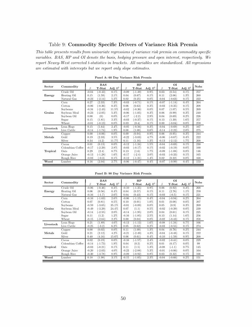
C.3 Commodity Specific Determinants
In addition to macroeconomic factors, we analyze the impact of commodity specific
variables on variance risk premia. We evaluate 3 variables considered to be important
in commodity markets: the basis, hedging pressure and open interest.
First, the theory of storage postulates that commodity prices are more volatile
when inventories are low, which motivates the inclusion of the basis. Given the
difficulties inherent in global inventory data (e.g. measurement errors, low reporting
frequency), we proxy inventories with the futures basis (BAS), defined as the ratio
of the second nearby futures contract over the first nearby contract. Note that
the theory of storage predicts the impact of inventory on realized variance only.
The theory is silent about implied variance, let alone variance risk premia. Hence,
evaluating the impact of inventory levels on variance risk premia is an empirical
question.
Second, it is also possible that the balance of short and long commercial hedgers
affects the market price of variance risk. Specifically, if variance risk premia are
negatively correlated with futures risk premia, we expect the slope estimate of
hedging pressure (HP) to be negative.17
Third, the recent debate on the causes of commodity price volatility points to
increased trading activities due to a growing number of financial investors. Hong
and Yogo (2012) have recently reported that open interest (OI) has strong predictive
power for subsequent price changes. However, some would argue that increased open
interest should reduce the cost of insurance as market participants are trading in
17This flows from the hedging pressure hypothesis, which predicts a positive relationship betweenhedging pressure and risk premia.
25
a fairly liquid market. A priori, it is not clear what effect open interest should
have on the market price of variance risk. Hence, it is interesting to investigate its
impact on variance risk premia as well. Both, the hedging position of commercial
and non-commercial traders and the open interest information are obtained from
the Commodity Futures Trading Commission (CFTC) and computed following the
methodology described in Hong and Yogo (2012).18
Table 9 reports results of univariate regressions of variance risk premia on the
commodity specific variables. Starting with the 60 day variance risk premia, we
observe that the basis is the most important commodity specific determinant of
variance risk premia with 11 significant coefficient estimates, 6 of which are positive.
Moreover, the basis can explain more than 11% of variations in variance risk premia
of soybeans and silver. As previously discussed, a positive relationship between bases
and variance risk premia, as reported for lumber and sugar, for example does not
necessarily invalidate the theory of storage but rather suggests that risk-neutral
variance is more responsive to changes in inventories than realized variance.19
Our evidence also indicates that hedging pressure significantly affects the
market price of variance risk of 3 commodities namely soybean oil, gold and orange
juice. In each of these markets, the coefficient estimates are negative, implying
that variance risk premia become “more” negative as short commercial hedgers
outnumber their long counterpart. It is instructive to bear in mind that the hedging
pressure theory predicts a positive relationship between hedging pressure and futures
risk premia. Hence, the weak negative correlation uncovered provides some evidence
of a negative correlation between futures risk premia and variance risk premia in
18The CFTC publishes several reports including futures only, and futures and options combinedreports. We use the futures report because of its longer sample period.
19The relationship between inventories and realized volatility has been studied among others bySymeonidis et al. (2012).
26
some commodity markets. However, it is also noteworthy that the sign of the hedging
pressure variable changes across markets.
Interestingly, we find that open interest growth has very little explanatory power
for explaining variations in variance risk premia. Thus the results obtained by Hong
and Yogo (2012) regarding open interest and futures prices do not carry over to
variance risk premia.
Overall, Panel A indicates that inventory levels are the most important
commodity specific determinants of variance risk premia. Panel B presents results
for 90 day variance risk premia leading to similar conclusions regarding the relative
importance of each commodity variable.
Together, Tables 7 through 9 reveal that both commodity and macroeconomic
factors determine variations in variance risk premia. Yet, we know little about the
relative contribution of each set of factors. To address this question, we combine
CPI, IP, DFSPD, TSPD, BAS, HP and OI in a single regression and evaluate their
respective contributions through the marginal R2 also employed by Longstaff et al.
(2011).20,21 More precisely, we divide the R2 of the regression with commodity
specific regressors only by that obtained with both commodity and macroeconomic
variables. By construction, a high marginal R2 indicates a high information content
of commodity specific variables for variance risk premia and vice versa. Column
“Marg R2” of Table 10 reveals that some commodities are highly affected by
commodity specific factors with marginal R2 reaching 82.1% for oats. We obtain
analogous, albeit more modest, results for natural gas (66.2%), soybeans (55.2%)
20We discard RGDP because of collinearity concerns. Using either RGDP or IP, we obtain verysimilar results. These results are available upon request.
21Results based on macroeconomic uncertainty instead of expectations yield similar results andare available upon request.
27
and soybean meal (61.6%).22 On average and across markets, commodity specific
factors supplement the explanatory power of macroeconomic factors by 34% (41.2%)
for variance risk premia over 60 (90) days.
In summary, our empirical results provide some support to the theoretical
predictions of Drechsler and Yaron (2011): variance risk premia respond to
macroeconomic uncertainty. Moreover, macroeconomic expectations account for a
substantial level of variations in the market price of variance risk. Notwithstanding
the prominence of macroeconomic factors, commodity specific variables enhance
our understanding of variance risk premia in some markets as highlighted by the
marginal R2 reported in Table 10.
D. Do Variance Risk Premia Predict Returns?
Over the past few years, gold has been widely considered as a safe haven, a store
of value and hedge against inflation. Tables 7 through 10 unequivocally show
that gold’s variance risk premium is mainly influenced by macroeconomic forecasts.
These observations brings us to ask an important question: does gold variance risk
premium contain information for future returns?
We focus specifically on gold for several reasons. First, Table 7 shows that
unlike most commodities, its variance risk premia is sensitive to each macroeconomic
variable employed. Second, the results obtained by combining macro and commodity
specific factors suggest that almost a quarter of variations in the variance risk
premium of gold can be explained. Moreover, almost 80% of the explanatory power
stems from macroeconomic rather than from commodity specific factors.
In the following, we assess the predictive power of gold’s 90 day variance risk
22Since the calculations involve R2 instead of its adjusted counterpart, the marginal R2 mustbe viewed as an upper limit of explanatory power gained by adding commodity specific factors.
28
premium for commodity returns over 4 horizons: 3, 6, 9 and 12 months. The most
closely related study to ours is that of Pan and Kang (2011), who demonstrate that
crude oil’s variance risk premium contains information for its future returns. Though
related, our aim is to investigate whether gold’s variance risk premium predicts not
only the returns of gold but also those of other commodities.
Studies on return predictability are often criticized on the grounds that their
findings suffer from either overlapping observations biases or the use of persistent
regressors.23 In order to address these concerns, we use non-overlapping variance
risk premia obtained by estimating 90 day variance risk premia once every quarter.24
Given our interest in predicting returns, we need a strictly ex-ante forecast of
variance risk premia. So far, the expected realized variance under the physical
measure has been estimated by using ex-post realized variance. However, to avoid
look ahead biases, we estimate expected realized variance by using an exponentially
weighted moving average model (EWMA) with smoothing constant λ equal to 0.94.
In this way, we rely on historical data only yielding truly out-of-sample forecasts.
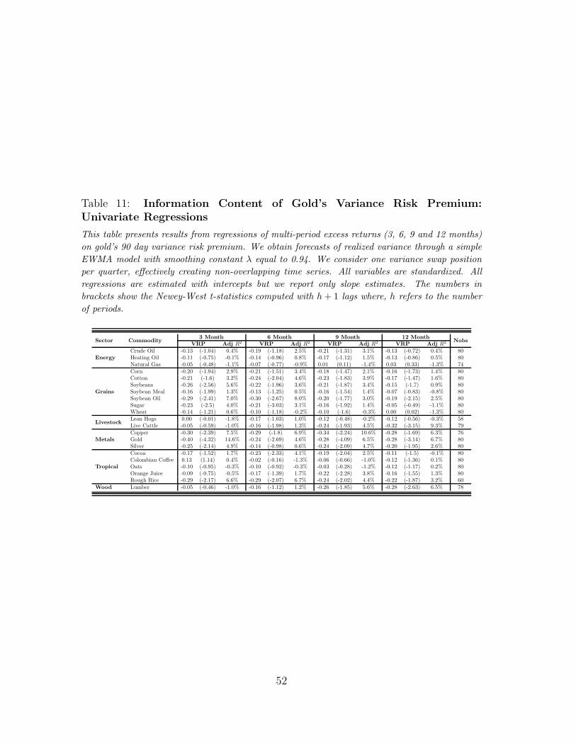
D.1 Univariate Analysis
To start, we conduct univariate analyses by simply regressing commodity spot
returns on gold’s variance risk premia:
Rt,t+h = α + βV RPt + εt (8)
where Rt,t+h is the excess return over the period t to t + h of the commodity
considered. V RPt refers to non-overlapping variance risk premia of gold at time
23See Ang and Bekaert (2007) and the references therein.24We show in Subsection E.1 that gold’s 90 day non-overlapping variance risk premium has a
first order auto-correlation close to zero, making it suitable for multi-period analyses.
29
t. εt denotes the error term.
The intuition is simple. If variance risk premia are equivalent to insurance
premia, we anticipate a negative relationship between variance risk premia and
returns: β < 0. The reason for this is that rational risk-averse investors purchase
insurance because they anticipate difficult macro-economic conditions for which,
they require higher expected returns. Table 11 summarizes the results of Regression
(8). For ease of comparison, we standardize all variables. We interpret a significant
slope coefficient as evidence for predictability. The predictive ability of gold’s
variance risk premium for its own returns manifests at all horizons. The strongest
results—in terms of magnitude, goodness of fit and significance—are obtained for
quarterly returns which is plausible as the variance risk premia employed have a
quarterly horizon as well.
Moreover, Table 11 shows that gold’s variance risk premium contains
information for future returns in as many as 13 other commodity markets. The
significantly negative coefficient estimates indicate that the predictive power is
apparent at all horizons for copper, soybeans, soybean oil and rough rice. The
explanatory power is also remarkable. For instance, gold’s variance risk premium
explains as much as 10% of the variations in copper’s returns, which is economically
sizable.
D.2 Multivariate Analysis
In the second step, we augment our baseline model with the basis and open interest,
two variables that have been shown to successfully predict commodity returns:
Rt,t+h = α + βV RPt + γBASt + δOIt + εt (9)
30
where Rt,t+h is the excess return over the period t to t + h of the commodity
considered. V RPt refers to non-overlapping variance risk premia of gold at time
t. BASt and OIt denote the basis and open interest of the commodity considered
calculated as in Hong and Yogo (2012). εt denotes the error term.
Since commodity prices are often considered to be mean-reverting, we anticipate
a positive (negative) relationship between the basis (inventory) and spot returns.
Recent evidence by Hong and Yogo (2012) points to the predictive power of open
interest growth for commodity returns. Therefore it is important to ascertain
whether open interest crowds out the information content of gold’s variance
risk premium found in the univariate regressions. Three outcomes are possible.
First, gold’s variance risk premium remains significant, indicating that it contains
important information for future returns. Second it becomes insignificant, implying
that traditional predictors crowd out its information content. Finally, it could
become significant even though insignificant in univariate regressions. Though
unlikely, this scenario may be due to omitted variable biases.
Table 12 indicates that despite the inclusion of traditional predictors, gold’s
variance risk premium remains significant for most commodities. The similarities—
both in terms of magnitude and sign—with the univariate regressions are striking.
The significance of gold’s variance risk premium, observed across all horizons in
copper, gold, soybeans, soybean oil and rough rice, is robust to the inclusion of
traditional predictors. Clearly, this result indicates that gold’s variance risk premium
contains useful information for returns above and beyond that of the basis and
open interest. We detect little evidence to suggest that the two predictors subsume
gold’s variance risk premium. In fact, this scenario occurs only for silver’s 12-month
returns. We also observe that gold’s variance risk premium becomes significant in the
31
coffee (12-month returns) and soybean meal (6 and 9 month returns) markets. The
positive signs of the basis and open interest are consistent with previous studies.
Surprisingly, we obtain somewhat weak evidence in favor of open interest. This
result is rather puzzling as Hong and Yogo (2012) demonstrate that open interest
has strong predictive power for commodity returns. We attribute these differences
to our shorter time period.
We further evaluate the contribution of gold’s variance risk premium by
comparing adjusted R2s of the augmented regression with and without gold’s
variance risk premium, which we report in the columns Adj R21 and Adj R2
2,
respectively. Intuitively, if the variance risk premium predicts future returns,
we anticipate that Adj R21 is greater than Adj R2
2. The evidence is compelling:
significant test statistics for gold’s variance risk premium are always accompanied
by improvements in explanatory power. The importance of gold’s variance risk
premium is most visible for copper: the explanatory power for 9-month returns
surges from−1.6% to 8.7% as we add gold’s variance risk premium to the regression.
In summary, Tables 11 and 12 document that gold’s variance risk premium
contains information for commodity future returns above and beyond that of
traditional predictors. Moreover, the predictive power extends to commodities
within and beyond the metal sector. These results might provide guidance for a
successful trading strategy that extracts signals from gold’s variance risk premium.
E. Robustness Analysis
In this section, we evaluate the robustness of our findings. To begin with, we analyze
the effect of overlapping observations on our main conclusions. Subsequently, we
focus on the temporal stability of the variance risk premia estimates.
32
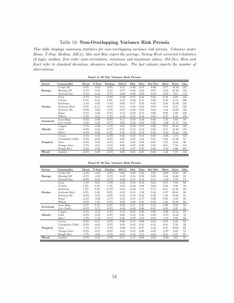
E.1 Non-Overlapping Samples
Although the various statistics displayed in Table 3 are compelling, they are subject
to a potential problem: we estimated realized variance on a rolling window basis.
It could be argued that because of the substantial amount of overlap in sampling
periods, our results may not be particularly informative. To address such concern,
we present summary statistics of non-overlapping variance risk premia in Table 13.
Overall, the results are quite similar to those reported in Table 3. Of course, some
differences are also observed. For some commodities such as lean hogs (60 day
horizon) and silver (90 day horizon), we find that variance risk is no longer priced
which might be a result of the substantially decreased number of observations.
It is interesting to note the sharp reduction in the autocorrelation of variance
risk premia. In particular, the fall in autocorrelation of gold’s 90 day variance risk
premium, from 0.97 to 0, provides further justification for using gold’s variance risk
premium as independent variable in the return predictability analysis presented in
Subsection D.
E.2 Subsample Analysis
In order to analyze the robustness of our results with respect to the observation
period, we partition our sample into 3 distinct periods: the first period ends in
November 2000, the second extends from December 2000 to November 2006 and
the third subsample runs from December 2006 onward. These periods are selected
because of their economic importance. The first subsample corresponds to a calm
and relatively uneventful period. The second period coincides with the increasing
financialization of commodities. Finally, the last subsample provides insights into
the dynamics of variance risk premia during the recent financial crisis.
33
We observe some differences between pre-crisis and post-crisis samples. For
example, in Table 13, variance risk (60 day) is priced in the soybeans market
from 2006 onward only. For silver, we find that its variance exhibits changes sign
over the subperiods. The 60 day variance risk premium is positive (1.2%) in the
first subsample and negative in the following subsamples (−1% and −2.6% for
the growth and crisis periods, respectively). These findings can explain why no
significant variance risk premium was found for the entire sample period. For some
commodities (e.g. soybean meal), the magnitude of variance risk premia during
the recent crisis is about twice as large as during the pre-crisis sample. This
observation confirms our finding that variance risk premia are negatively related
to MFIV . Overall, our conclusion of negative variance risk premia holds over the
recent economic downturn.
IV Conclusion
This paper investigates the market price of variance risk in 21 commodity markets
from 1989 to 2011. Using synthetically constructed variance swaps that mature
in 60 and 90 calendar days, we present evidence of significantly negative variance
risk premia. Although generally similar, we detect sign-switching behavior across
maturities (e.g. lean hogs) or subsamples (e.g. silver) in some markets, most likely
due to term-structure effects or time variations in variance risk premia.
We further analyze the economic determinants of variance risk premia and
document a strong relation between macroeconomic expectations, uncertainty and
variance risk premia. Moreover, we find that commodity specific variables enhance
our understanding of variance risk premia dynamics, indicating that both systematic
34
and idiosyncratic factors impact variance risk premia.
Assessing the information content of gold’s variance risk premium for
commodity returns, we find evidence of predictability in several markets. The large
and negative slope coefficients observed in most markets underline the economic
significance of the relationship. The information contained in gold’s variance risk
premium are above and beyond that of traditional predictors such as the basis and
open interest.
Our study can be extended in several directions. First, as commodity option
markets become more liquid, it would be interesting to study the term-structure of
variance risk premia by considering variance risk swaps of longer maturities. Second,
our study does not address the issue of jump risk premia. Finally, our analysis
reveals large cross-sectional variations in variance risk premia. Understanding the
determinants of these variations is another interesting research question.
35
References
Andersen, T., Bollerslev, T., and Diebold, F. (2009). Parametric and nonparametric
volatility measurement. Handbook of Financial Econometrics: Tools and
Techniques, 1:67.
Ang, A. and Bekaert, G. (2007). Stock return predictability: Is it there? Review of
Financial Studies, 20(3):651–707.
Back, J., Prokopczuk, M., and Rudolf, M. (2013). Seasonality and the valuation of
commodity options. Journal of Banking & Finance, 37(2):273–290.
Bakshi, G. and Kapadia, N. (2003a). Delta-hedged gains and the negative market
volatility risk premium. Review of Financial Studies, 16(2):527–566.
Bakshi, G. and Kapadia, N. (2003b). Volatility risk premiums embedded in
individual equity options. Journal of Derivatives, 11(1):45–54.
Bakshi, G. and Madan, D. (2006). A theory of volatility spreads. Management
Science, 52(12):1945–1956.
Barnea, A. and Hogan, R. (2012). Quantifying the variance risk premium in VIX
options. Journal of Portfolio Management, 38(3):143–148.
Barone-Adesi, G. and Whaley, R. (1987). Efficient analytic approximation of
american option values. Journal of Finance, 42(2):301–320.
Black, F. (1976). The pricing of commodity contracts. Journal of Financial
Economics, 3(1):167–179.
Bollerslev, T., Gibson, M., and Zhou, H. (2011a). Dynamic estimation of volatility
36
risk premia and investor risk aversion from option-implied and realized volatilities.
Journal of Econometrics, 160(1):235–245.
Bollerslev, T., Marrone, J., Xu, L., and Zhou, H. (2011b). Stock return predictability
and variance risk premia: statistical inference and international evidence. Duke
University Working Paper Series.
Bollerslev, T., Tauchen, G., and Zhou, H. (2009). Expected stock returns and
variance risk premia. Review of Financial Studies, 22(11):4463–4492.
Branger, N. and Schlag, C. (2008). Can tests based on option hedging errors correctly
identify volatility risk premia? Journal of Financial and Quantitative Analysis,
43(4):1055–1090.
Britten-Jones, M. and Neuberger, A. (2000). Option prices, implied price processes,
and stochastic volatility. Journal of Finance, 55(2):839–866.
Broadie, M., Chernov, M., and Johannes, M. (2007). Model specification and risk
premia: Evidence from futures options. Journal of Finance, 62(3):1453–1490.
Brooks, C. and Prokopczuk, M. (2011). The dynamics of commodity prices. ICMA
Centre Discussion Paper.
Buraschi, A. and Whelan, P. (2011). Macroeconomic uncertainty, difference in
beliefs, and bond risk premia. Imperial College Discussion Paper.
Carr, P. and Wu, L. (2009). Variance risk premiums. Review of Financial Studies,
22(3):1311–1341.
Coval, J. and Shumway, T. (2001). Expected option returns. Journal of Finance,
56(3):983–1009.
37
Demeterfi, K., Derman, E., Kamal, M., and Zou, J. (1999). A guide to volatility
and variance swaps. Journal of Derivatives, 6(4):9–32.
Doran, J. and Ronn, E. (2008). Computing the market price of volatility risk in the
energy commodity markets. Journal of Banking & Finance, 32(12):2541–2552.
Drechsler, I. (2012). Uncertainty, time-varying fear, and asset prices. Forthcoming
in Journal of Finance.
Drechsler, I. and Yaron, A. (2011). What’s vol got to do with it. Review of Financial
Studies, 24(1):1–45.
Driessen, J., Maenhout, P., and Vilkov, G. (2009). The price of correlation risk:
Evidence from equity options. Journal of Finance, 64(3):1377–1406.
Eraker, B., Johannes, M., and Polson, N. (2003). The impact of jumps in volatility
and returns. Journal of Finance, 58(3):1269–1300.
Guo, D. (1998). The risk premium of volatility implicit in currency options. Journal
of Business & Economic Statistics, 16(4):498–507.
Hafner, R. andWallmeier, M. (2007). Volatility as an asset class: European evidence.
European Journal of Finance, 13(7):621–644.
Heston, S. (1993). A closed-form solution for options with stochastic volatility
with applications to bond and currency options. Review of Financial Studies,
6(2):327–343.
Hong, H. and Yogo, M. (2012). What does futures market interest tell us about the
macroeconomy and asset prices? Journal of Financial Economics, 105(3):473–
490.
38
Jiang, G. and Tian, Y. (2005). The model-free implied volatility and its information
content. Review of Financial Studies, 18(4):1305–1342.
Koijen, R., Moskowitz, T., Pedersen, L., and Vrugt, E. (2012). Carry. Working
Paper.
Longstaff, F., Pan, J., Pedersen, L., and Singleton, K. (2011). How sovereign is
sovereign credit risk? American Economic Journal: Macroeconomics, 3(2):75–
103.
Low, B. and Zhang, S. (2005). The volatility risk premium embedded in currency
options. Journal of Financial and Quantitative Analysis, 40(4):803–832.
Mueller, P., Vedolin, A., and Yen, Y. (2011). Bond variance risk premia. LSE
Working Paper.
Pan, J. (2002). The jump-risk premia implicit in options: Evidence from an
integrated time-series study. Journal of Financial Economics, 63(1):3–50.
Pan, X. and Kang, S. (2011). Do the variance risk premia predict commodity futures
returns? Evidence from the crude oil market. McGill University Working Paper.
Simon, D. (2010). Examination of long-term bond iShare option selling strategies.
Journal of Futures Markets, 30(5):465–489.
Suenaga, H., Smith, A., and Williams, J. (2008). Volatility dynamics of NYMEX
natural gas futures prices. Journal of Futures Markets, 28(5):438–463.
Symeonidis, L., Prokopczuk, M., Brooks, C., and Lazar, E. (2012). Futures basis,
inventory and commodity price volatility: An empirical analysis. Economic
Modelling, 29(6):2651–2663.
39
Trolle, A. and Schwartz, E. (2009). Unspanned stochastic volatility and the pricing
of commodity derivatives. Review of Financial Studies, 22(11):4423–4461.
Trolle, A. and Schwartz, E. (2010). Variance risk premia in energy commodities.
Journal of Derivatives, 17(3):15–32.
Wang, H., Zhou, H., and Zhou, Y. (2010). Credit default swap spreads and variance
risk premia. Working Paper.
Wang, Z., Fausti, S., and Qasmi, B. (2011). Variance risk premiums and predictive
power of alternative forward variances in the corn market. Journal of Futures
Markets, 32(6):587–608.
40
01/01/1991 01/01/2000 01/01/2009
0.2
0.4
0.6
0.8
1
1.2
Crude Oil
Var
ianc
e
01/01/1991 01/01/2000 01/01/2009
0.1
0.2
0.3
0.4
0.5
0.6
Soybean
Var
ianc
e
01/01/1991 01/01/2000 01/01/2009
0.02
0.04
0.06
0.08
0.1
0.12
0.14
Live Cattle
Var
ianc
e
01/01/1991 01/01/2000 01/01/2009
0.2
0.4
0.6
0.8
1
Copper
Var
ianc
e
01/01/1991 01/01/2000 01/01/2009
0.1
0.2
0.3
0.4
0.5
Cocoa
Var
ianc
e
01/01/1991 01/01/2000 01/01/2009
0.1
0.2
0.3
0.4
0.5
Lumber
Var
ianc
e
MFIVRV
MFIVRV
MFIVRV
MFIVRV
MFIVRV
MFIVRV
Figure 1: Time Series of Realized Variance and Model-Free Implied
Variance
This figure displays time series of realized and model-free implied variances for crude oil, soybean,
live cattle, copper, cocoa, lumber over a 60 day horizon. The blue and green lines represent
model-free implied and realized variances, respectively. The difference between realized and implied
variance is the variance risk premium.
41
Table 1: Overview of Commodities
This table lists all commodities considered. The first two columns report the sector and name
of specific commodities. The third column displays the exchange where the futures and options
contracts of the commodity are traded. The last two columns contain the available maturity months
and minimum tick sizes of the options contracts as reported by the relevant exchange.
Corn CBOT January, March, May, July, September, November, December 0.25Cotton ICE March, May, July, October, December 0.01Soybeans CBOT January, March, May, July, August, September, November 0.25Soybean Meal CBOT January, March, May, July, August, September, October, December 0.1Soybean Oil CBOT January, March, May, July, August, September, October, December 0.01Sugar ICE March, May, July, October, December 0.01Wheat CBOT March, May, July, September, December 0.25
LivestockLean Hogs CME Febuary, April, June, July, August, October, December 0.025Live Cattle CME Febuary, April, June, August, October, December 0.025
MetalsCopper COMEX March, May, July, September, December 0.0005Gold COMEX Febuary, April, June, August, October, December 0.1Silver COMEX March, May, July, September, December 0.5
Tropical
Cocoa ICE March, May, July, September, December 1Colombian Coffee ICE March, May, July, September, December 0.05Oats CBOT March, May, July, September, December 0.25Orange Juice ICE January, March, May, July, September, November 0.05Rough Rice CBOT January, March, May, July, September, November 0.05
Wood Lumber CME January, March, May, July, September, November 0.1
42
Table 2: Description of Options Data
This table summarizes information about the OTM options data. For each commodity, we only
retain OTM options that mature between 30 and 120 calendar days. The first two columns report
the sector and name of specific commodities. Columns “Starting Date” and “Ending Date” indicate
the beginning and end of the sample, respectively. “Days” reports the number of observation days
in the sample. The last two columns show the average number of OTM calls and puts on each
trading day, respectively.
Sector Commodity Starting Date Ending Date Days Calls Puts
EnergyCrude Oil 16 Jan 89 02 Sep 11 5640 27 22Heating Oil 11 Jan 89 14 Sep 11 5660 29 24Natural Gas 02 Oct 92 14 Sep 11 4740 51 27
Grains
Corn 24 Feb 89 07 Oct 11 5691 19 13Cotton 30 Jan 90 16 Nov 07 4449 20 15Soybeans 24 Feb 89 07 Oct 11 5692 20 14Soybean Meal 24 Feb 89 14 Oct 11 5686 8 5Soybean Oil 24 Feb 89 07 Oct 11 5651 13 11Sugar 06 Mar 90 04 Oct 11 5372 26 17Wheat 24 Feb 89 07 Oct 11 5692 18 13
LivestockLean Hogs 01 Feb 85 13 May 11 6612 7 12Live Cattle 30 Oct 84 28 Feb 11 6630 9 11
MetalsCopper 12 Dec 89 11 Oct 11 5461 12 14Gold 03 Jan 89 11 Oct 11 5704 16 13Silver 03 Mar 89 26 Oct 11 5673 24 32
Tropical
Cocoa 06 Mar 90 23 Sep 11 5384 10 6Colombian Coffee 05 Mar 90 30 Sep 11 5390 5 19Oats 01 May 90 12 Aug 11 5344 7 5Orange Juice 02 Mar 90 07 Oct 11 5370 8 4Rough Rice 10 Apr 92 14 Jul 11 4832 9 6
Wood Lumber 05 Jun 87 15 Nov 10 5680 10 7
43
Table 3: Variance Risk Premia
This table presents summary statistics of the estimated commodity variance risk premia. Columns
entitled Mean, T-Stat, Median, AR(1), Min and Max report the average, Newey-West corrected
t-statistic (same lag length as the maturity of the swap), median, first order auto-correlation,
minimum and maximum variance risk premia. The last four columns display the standard
deviation, skewness, kurtosis and number of observations, respectively. Panel A presents the results
for a horizon of 60 days, Panel B for a horizon of 90 days.
Panel A: 60 Day Variance risk premia
Sector Commodity Mean T-Stat Median AR(1) Min Max Std Dev Skew Kurt Obs