62
Variation and Change in Online Social Networks Jacob Eisenstein @jacobeisenstein Georgia Institute of Technology April 21, 2017
| Date post: | 19-May-2018 |
| Category: |
Documents |
| Upload: | vuongkhuong |
| View: | 216 times |
| Download: | 2 times |
Variation and Change in OnlineSocial Networks
Jacob Eisenstein@jacobeisenstein
Georgia Institute of Technology
April 21, 2017
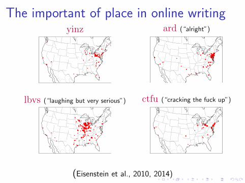
The important of place in online writingyinz ard (“alright”)
lbvs (“laughing but very serious”) ctfu (“cracking the fuck up”)
(Eisenstein et al., 2010, 2014)
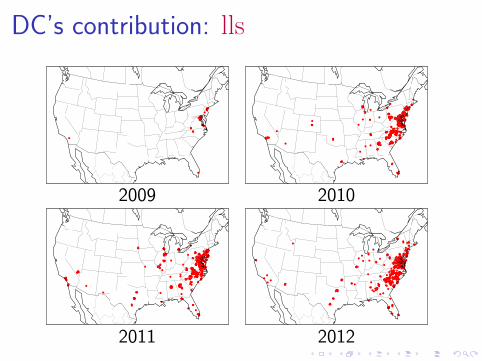
DC’s contribution: lls
2009 2010
2011 2012
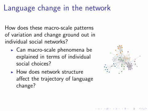
Language change in the network
How does these macro-scale patternsof variation and change ground out inindividual social networks?
I Can macro-scale phenomena beexplained in terms of individualsocial choices?
I How does network structureaffect the trajectory of languagechange?
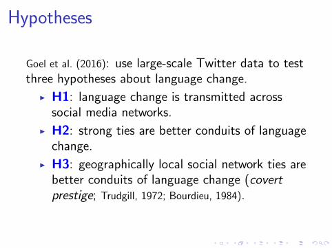
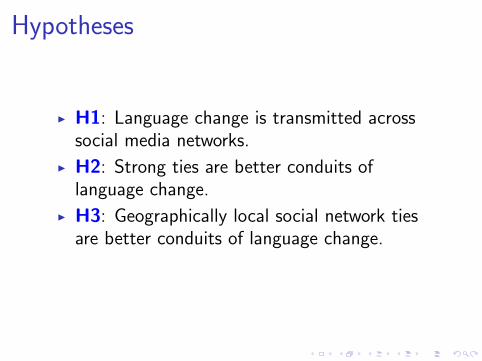
Hypotheses
Goel et al. (2016): use large-scale Twitter data to testthree hypotheses about language change.
I H1: language change is transmitted acrosssocial media networks.
I H2: strong ties are better conduits of languagechange.
I H3: geographically local social network ties arebetter conduits of language change (covertprestige; Trudgill, 1972; Bourdieu, 1984).
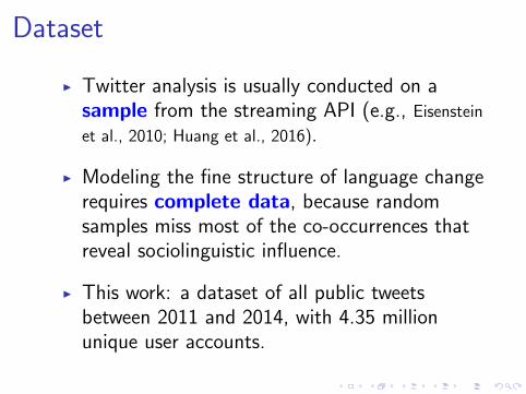
Dataset
I Twitter analysis is usually conducted on asample from the streaming API (e.g., Eisenstein
et al., 2010; Huang et al., 2016).
I Modeling the fine structure of language changerequires complete data, because randomsamples miss most of the co-occurrences thatreveal sociolinguistic influence.
I This work: a dataset of all public tweetsbetween 2011 and 2014, with 4.35 millionunique user accounts.
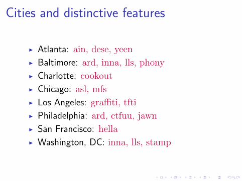
Cities and distinctive features
I Atlanta: ain, dese, yeen
I Baltimore: ard, inna, lls, phony
I Charlotte: cookout
I Chicago: asl, mfs
I Los Angeles: graffiti, tfti
I Philadelphia: ard, ctfuu, jawn
I San Francisco: hella
I Washington, DC: inna, lls, stamp
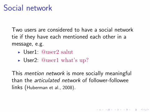
Social network
Two users are considered to have a social networktie if they have each mentioned each other in amessage, e.g.
I User1: @user2 salut
I User2: @user1 what’s up?
This mention network is more socially meaningfulthan the articulated network of follower-followeelinks (Huberman et al., 2008).
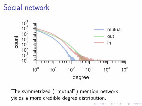
Social network
100 101 102 103 104 105
degree
100101102103104105106107
coun
t
mutualoutin
The symmetrized (“mutual”) mention networkyields a more credible degree distribution.
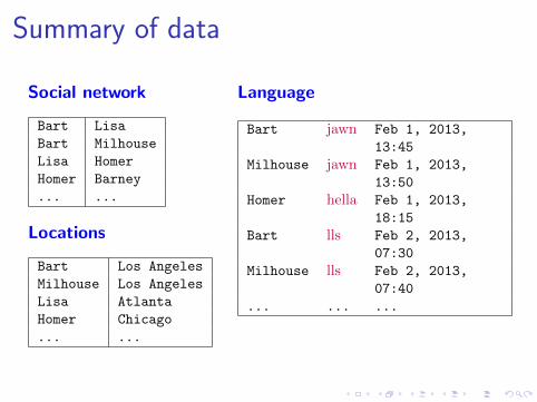
Summary of data
Social network
Bart Lisa
Bart Milhouse
Lisa Homer
Homer Barney
... ...
Locations
Bart Los Angeles
Milhouse Los Angeles
Lisa Atlanta
Homer Chicago
... ...
Language
Bart jawn Feb 1, 2013,
13:45
Milhouse jawn Feb 1, 2013,
13:50
Homer hella Feb 1, 2013,
18:15
Bart lls Feb 2, 2013,
07:30
Milhouse lls Feb 2, 2013,
07:40
... ... ...
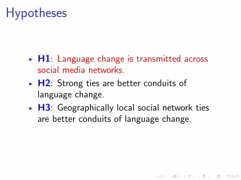
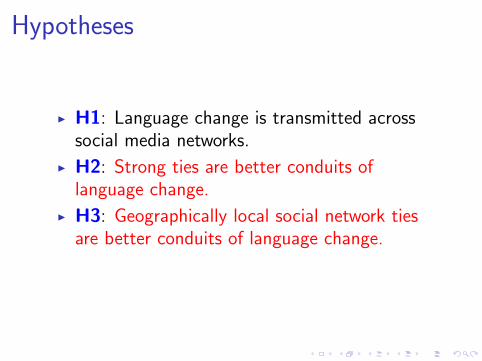
Hypotheses
I H1: Language change is transmitted acrosssocial media networks.
I H2: Strong ties are better conduits oflanguage change.
I H3: Geographically local social network tiesare better conduits of language change.
Hypotheses
I H1: Language change is transmitted acrosssocial media networks.
I H2: Strong ties are better conduits oflanguage change.
I H3: Geographically local social network tiesare better conduits of language change.
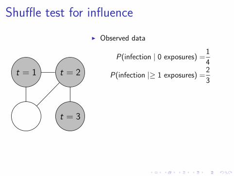
Shuffle test for influence
t = 1 t = 2
t = 3
I Observed data
P(infection | 0 exposures) =1
4
P(infection |≥ 1 exposures) =2
3
I Randomized data
P(infection | 0 exposures) =2
4
,1
4, . . .
P(infection |≥ 1 exposures) =1
2
,2
3, . . .
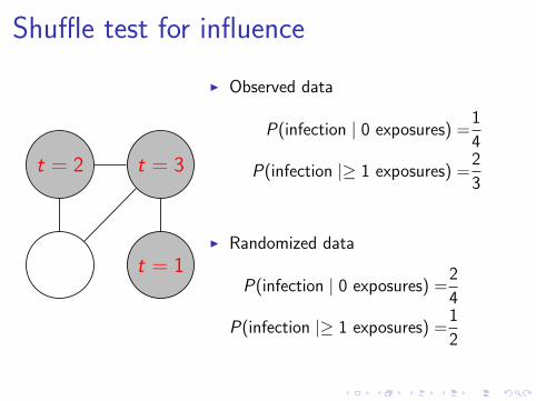
Shuffle test for influence
t = 2 t = 3
t = 1
I Observed data
P(infection | 0 exposures) =1
4
P(infection |≥ 1 exposures) =2
3
I Randomized data
P(infection | 0 exposures) =2
4
,1
4, . . .
P(infection |≥ 1 exposures) =1
2
,2
3, . . .
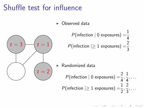
Shuffle test for influence
t = 3 t = 1
t = 2
I Observed data
P(infection | 0 exposures) =1
4
P(infection |≥ 1 exposures) =2
3
I Randomized data
P(infection | 0 exposures) =2
4,
1
4, . . .
P(infection |≥ 1 exposures) =1
2,
2
3, . . .
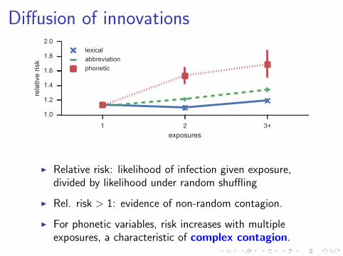
Diffusion of innovations
1 2 3+exposures
1.0
1.2
1.4
1.6
1.8
2.0re
lativ
e ris
k
lexicalabbreviationphonetic
I Relative risk: likelihood of infection given exposure,divided by likelihood under random shuffling
I Rel. risk > 1: evidence of non-random contagion.
I For phonetic variables, risk increases with multipleexposures, a characteristic of complex contagion.

Hypotheses
I H1: Language change is transmitted acrosssocial media networks.
I H2: Strong ties are better conduits oflanguage change.
I H3: Geographically local social network tiesare better conduits of language change.
Hypotheses
I H1: Language change is transmitted acrosssocial media networks.
I H2: Strong ties are better conduits oflanguage change.
I H3: Geographically local social network tiesare better conduits of language change.
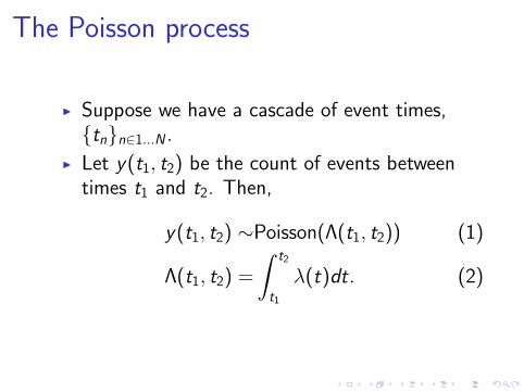
The Poisson process
I Suppose we have a cascade of event times,{tn}n∈1...N .
I Let y(t1, t2) be the count of events betweentimes t1 and t2. Then,
y(t1, t2) ∼Poisson(Λ(t1, t2)) (1)
Λ(t1, t2) =
∫ t2
t1
λ(t)dt. (2)
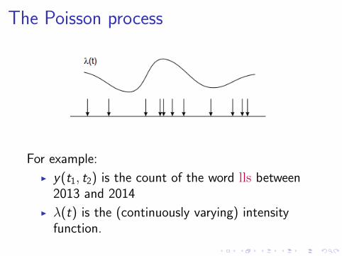
The Poisson process
For example:
I y(t1, t2) is the count of the word lls between2013 and 2014
I λ(t) is the (continuously varying) intensityfunction.
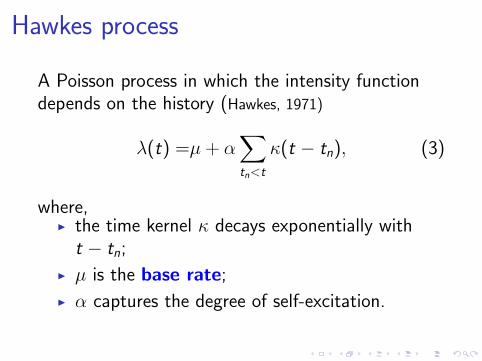
Hawkes process
A Poisson process in which the intensity functiondepends on the history (Hawkes, 1971)
λ(t) =µ + α∑tn<t
κ(t − tn), (3)
where,I the time kernel κ decays exponentially witht − tn;
I µ is the base rate;
I α captures the degree of self-excitation.
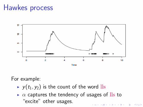
Hawkes process
For example:
I y(t1, y2) is the count of the word lls
I α captures the tendency of usages of lls to“excite” other usages.
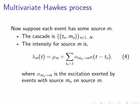
Multivariate Hawkes process
Now suppose each event has some source m.
I The cascade is {(tn,mn)}n∈1...N .
I The intensity for source m is,
λm(t) = µm +∑tn<t
αmn→mκ(t − tn), (4)
where αmn→m is the excitation exerted byevents with source mn on source m.
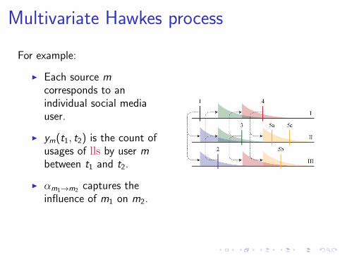
Multivariate Hawkes process
For example:
I Each source mcorresponds to anindividual social mediauser.
I ym(t1, t2) is the count ofusages of lls by user mbetween t1 and t2.
I αm1→m2 captures theinfluence of m1 on m2.
Parametric Hawkes process
The infection parameters are a linear function ofshared features of each pair of individuals,
αm1→m2= θ>f (m1 → m2). (5)
I We now need estimate only #|θ| parameters,rather than M2.
I We can use features to test hypotheses aboutwhat types of dyads are influential.
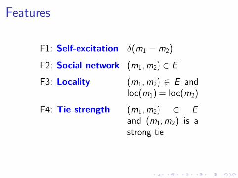
Features
F1: Self-excitation δ(m1 = m2)
F2: Social network (m1,m2) ∈ E
F3: Locality (m1,m2) ∈ E andloc(m1) = loc(m2)
F4: Tie strength (m1,m2) ∈ Eand (m1,m2) is astrong tie
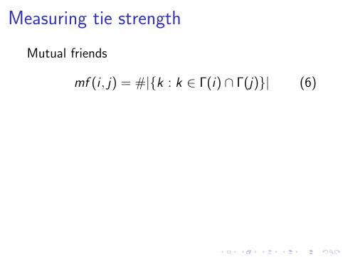
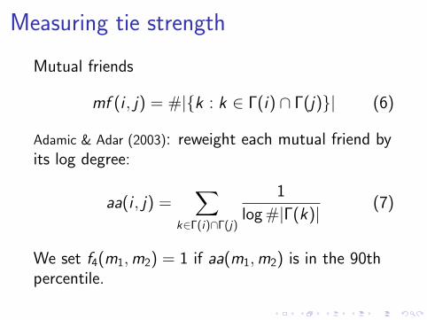
Measuring tie strength
Mutual friends
mf (i , j) = #|{k : k ∈ Γ(i) ∩ Γ(j)}| (6)
Adamic & Adar (2003): reweight each mutual friend byits log degree:
aa(i , j) =∑
k∈Γ(i)∩Γ(j)
1
log #|Γ(k)|(7)
We set f4(m1,m2) = 1 if aa(m1,m2) is in the 90thpercentile.
Measuring tie strength
Mutual friends
mf (i , j) = #|{k : k ∈ Γ(i) ∩ Γ(j)}| (6)
Adamic & Adar (2003): reweight each mutual friend byits log degree:
aa(i , j) =∑
k∈Γ(i)∩Γ(j)
1
log #|Γ(k)|(7)
We set f4(m1,m2) = 1 if aa(m1,m2) is in the 90thpercentile.
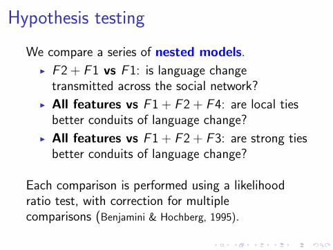
Hypothesis testing
We compare a series of nested models.
I F2 + F1 vs F1: is language changetransmitted across the social network?
I All features vs F1 + F2 + F4: are local tiesbetter conduits of language change?
I All features vs F1 + F2 + F3: are strong tiesbetter conduits of language change?
Each comparison is performed using a likelihoodratio test, with correction for multiplecomparisons (Benjamini & Hochberg, 1995).
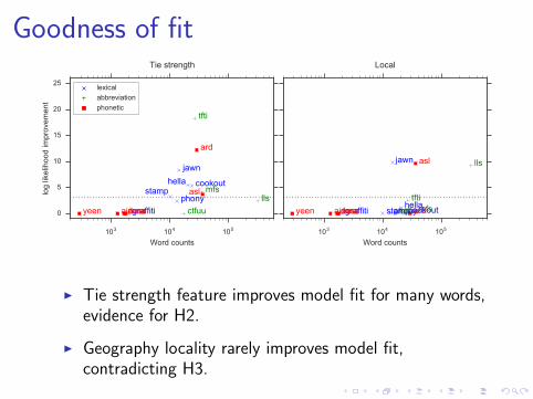
Goodness of fit
103 104 105
Word counts
0
5
10
15
20
25
log
likel
ihoo
d im
prov
emen
t
cookout
graffiti
hella
jawn
phonystamp
ctfuu
llsmfs
tfti
ain
ard
asl
deseinnayeen
Tie strength
lexical
abbreviation
phonetic
103 104 105
Word counts
cookoutgraffitihella
jawn
phonystampctfuu
lls
mfstfti
ain ard
asl
deseinnayeen
Local
I Tie strength feature improves model fit for many words,evidence for H2.
I Geography locality rarely improves model fit,contradicting H3.
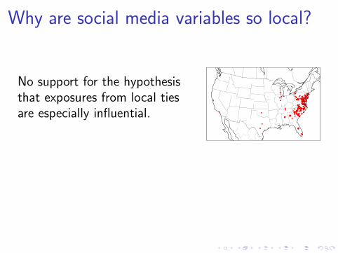
Why are social media variables so local?
No support for the hypothesisthat exposures from local tiesare especially influential.
But! Most exposures are local. Two reasons:
1. Most ties are local
2. Audience design (Pavalanathan & Eisenstein, 2015)
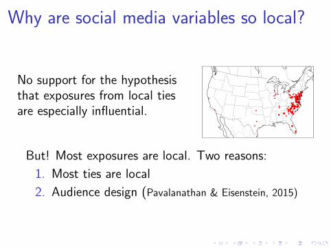
Why are social media variables so local?
No support for the hypothesisthat exposures from local tiesare especially influential.
But! Most exposures are local. Two reasons:
1. Most ties are local
2. Audience design (Pavalanathan & Eisenstein, 2015)
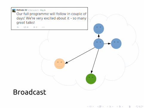
Broadcast
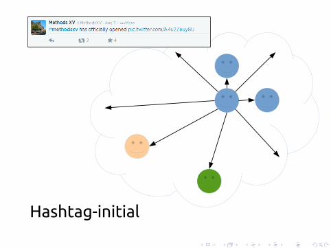
Hashtag-initial
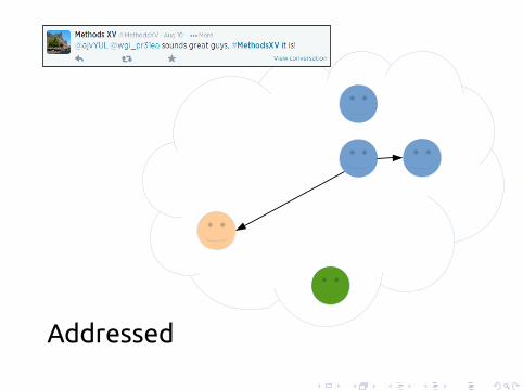
Addressed
Logistic regression
I Dependent variable: does the tweet containa non-standard, geographically-specific word(e.g., lbvs, hella, jawn)
I PredictorsI Message type: broadcast, addressed, #-initialI Controls: message length, author statistics
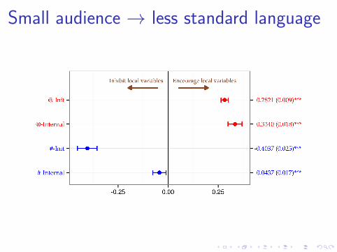
Small audience → less standard language
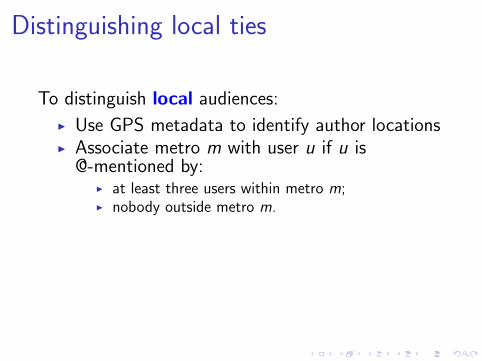
Distinguishing local ties
To distinguish local audiences:
I Use GPS metadata to identify author locationsI Associate metro m with user u if u is
@-mentioned by:I at least three users within metro m;I nobody outside metro m.
The social network lets us impute the locations ofunknown users from the 1-2% of users who revealtheir GPS! (Sadilek et al., 2012)
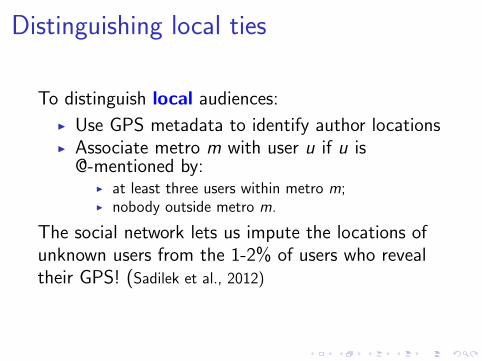
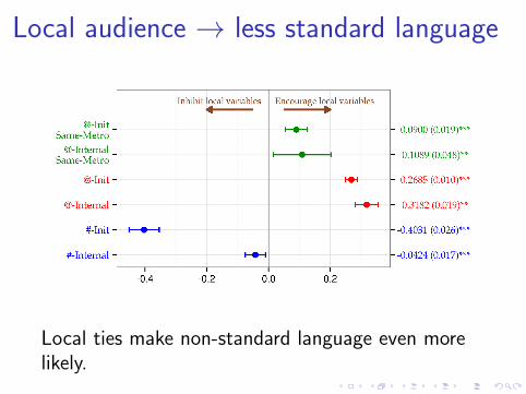
Local audience → less standard language
Local ties make non-standard language even morelikely.
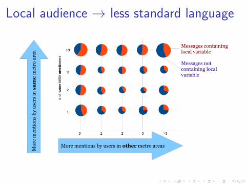
Local audience → less standard languageM
ore
men
tion
s by
use
rs in
same
met
ro a
rea
More mentions by users in other metro areas
Messages containing local variable
Messages not containing local variable
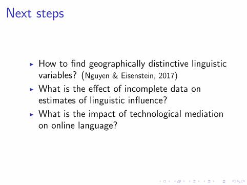
Next steps
I How to find geographically distinctive linguisticvariables? (Nguyen & Eisenstein, 2017)
I What is the effect of incomplete data onestimates of linguistic influence?
I What is the impact of technological mediationon online language?
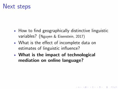
Next steps
I How to find geographically distinctive linguisticvariables? (Nguyen & Eisenstein, 2017)
I What is the effect of incomplete data onestimates of linguistic influence?
I What is the impact of technologicalmediation on online language?
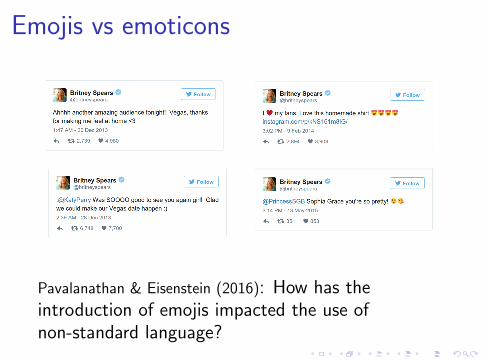
Emojis vs emoticons
Pavalanathan & Eisenstein (2016): How has theintroduction of emojis impacted the use ofnon-standard language?
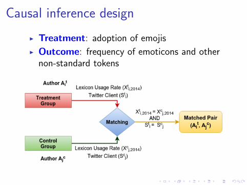
Causal inference design
I Treatment: adoption of emojis
I Outcome: frequency of emoticons and othernon-standard tokens
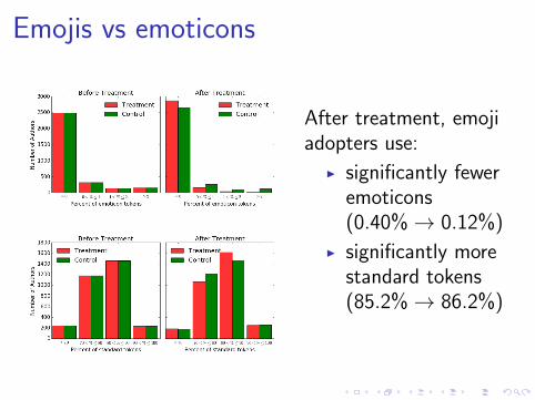
Emojis vs emoticons
After treatment, emojiadopters use:
I significantly feweremoticons(0.40%→ 0.12%)
I significantly morestandard tokens(85.2%→ 86.2%)
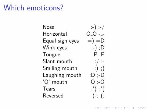
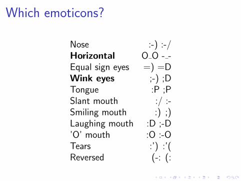
Which emoticons?
Nose :-) :-/Horizontal O O - -Equal sign eyes =) =DWink eyes ;-) ;DTongue :P ;PSlant mouth :/ :-Smiling mouth :) ;)Laughing mouth :D ;-D’O’ mouth :O :-OTears :’) :’(Reversed (-: (:
Which emoticons?
Nose :-) :-/Horizontal O O - -Equal sign eyes =) =DWink eyes ;-) ;DTongue :P ;PSlant mouth :/ :-Smiling mouth :) ;)Laughing mouth :D ;-D’O’ mouth :O :-OTears :’) :’(Reversed (-: (:
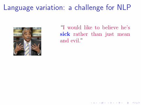
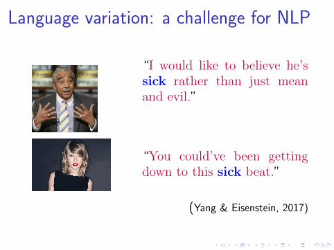
Language variation: a challenge for NLP
“I would like to believe he’ssick rather than just meanand evil.”
“You could’ve been gettingdown to this sick beat.”
(Yang & Eisenstein, 2017)
Language variation: a challenge for NLP
“I would like to believe he’ssick rather than just meanand evil.”
“You could’ve been gettingdown to this sick beat.”
(Yang & Eisenstein, 2017)
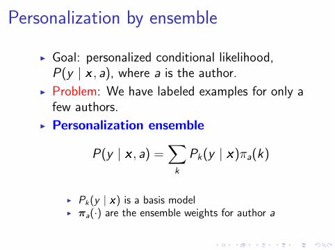
Personalization by ensemble
I Goal: personalized conditional likelihood,P(y | x , a), where a is the author.
I Problem: We have labeled examples for only afew authors.
I Personalization ensemble
P(y | x , a) =∑k
Pk(y | x)πa(k)
I Pk(y | x) is a basis modelI πa(·) are the ensemble weights for author a
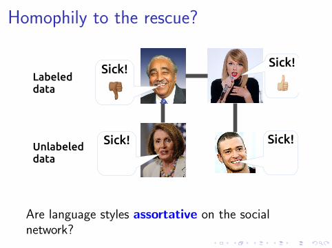
Homophily to the rescue?
Sick! Sick!
Sick!Sick!
Labeled data
Unlabeled data
Are language styles assortative on the socialnetwork?
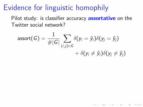
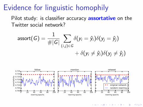
Evidence for linguistic homophilyPilot study: is classifier accuracy assortative on theTwitter social network?
assort(G ) =1
#|G |∑
(i ,j)∈G
δ(yi = yi)δ(yj = yj)
+ δ(yi 6= yi)δ(yj 6= yj)
0 20 40 60 80 100rewiring epochs
0.7000.7050.7100.7150.7200.7250.7300.735
asso
rtativ
ity
follow
0 20 40 60 80 100rewiring epochs
mention
0 20 40 60 80 100rewiring epochs
retweet
original networkrandom rewiring
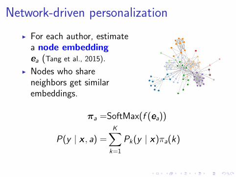
Network-driven personalization
I For each author, estimatea node embeddingea (Tang et al., 2015).
I Nodes who shareneighbors get similarembeddings.
πa =SoftMax(f (ea))
P(y | x , a) =K∑
k=1
Pk(y | x)πa(k)
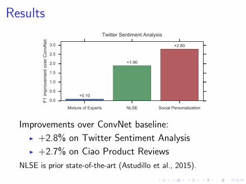
Results
Mixture of Experts NLSE Social Personalization
0.0
0.5
1.0
1.5
2.0
2.5
3.0F1
impr
ovem
ent o
ver C
onvN
et
+0.10
+1.90
+2.80
Twitter Sentiment Analysis
Improvements over ConvNet baseline:
I +2.8% on Twitter Sentiment Analysis
I +2.7% on Ciao Product Reviews
NLSE is prior state-of-the-art (Astudillo et al., 2015).
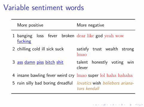
Variable sentiment words
More positive More negative
1 banging loss fever brokenfucking
dear like god yeah wow
2 chilling cold ill sick suck satisfy trust wealth stronglmao
3 ass damn piss bitch shit talent honestly voting winclever
4 insane bawling fever weird cry lmao super lol haha hahaha
5 ruin silly bad boring dreadful lovatics wish beliebers ariana-tors kendall
Conclusions
I Internet media continues to create new socialconfigurations, new subcultures, and newcommunicative affordances.
I New opportunities for studying themicro-foundations of language change.
I A future of blurred lines: online vs IRL, humancontrol vs autonomy, text vs speech.
Acknowledgments
I Collaborators: Ming-Wei Chang, FernandoDiaz, Naman Goyal, Rahul Goel, VinodhKrishnan, John Paparrizos, UmashanthiPavalanathan, Sandeep Soni, Hanna Wallach,Yi Yang
I Sponsors: National Science Foundation, AirForce Office of Scientific Research, NationalInstitutes for Health, Microsoft Research.
References IAdamic, L. A. & Adar, E. (2003). Friends and neighbors on the web. Social networks, 25(3), 211–230.
Astudillo, R. F., Amir, S., Lin, W., Silva, M., & Trancoso, I. (2015). Learning word representations from scarce andnoisy data with embedding sub-spaces. In Proceedings of the Association for Computational Linguistics(ACL), Beijing.
Benjamini, Y. & Hochberg, Y. (1995). Controlling the false discovery rate: a practical and powerful approach tomultiple testing. Journal of the Royal Statistical Society. Series B (Methodological), 289–300.
Bourdieu, P. (1984). Distinction: A social critique of the judgement of taste. Harvard University Press.
Eisenstein, J., O’Connor, B., Smith, N. A., & Xing, E. P. (2010). A latent variable model for geographic lexicalvariation. In Proceedings of Empirical Methods for Natural Language Processing (EMNLP), (pp. 1277–1287).
Eisenstein, J., O’Connor, B., Smith, N. A., & Xing, E. P. (2014). Diffusion of lexical change in social media. PLoSONE, 9.
Goel, R., Soni, S., Goyal, N., Paparrizos, J., Wallach, H., Diaz, F., & Eisenstein, J. (2016). The social dynamics oflanguage change in online networks. In The International Conference on Social Informatics (SocInfo).
Hawkes, A. G. (1971). Spectra of some self-exciting and mutually exciting point processes. Biometrika, 58(1),83–90.
Huang, Y., Guo, D., Kasakoff, A., & Grieve, J. (2016). Understanding us regional linguistic variation with twitterdata analysis. Computers, Environment and Urban Systems, 59, 244–255.
Huberman, B., Romero, D. M., & Wu, F. (2008). Social networks that matter: Twitter under the microscope.First Monday, 14(1).
Nguyen, D. & Eisenstein, J. (2017). A kernel independence test for geographical language variation.Computational Linguistics, in press.
Pavalanathan, U. & Eisenstein, J. (2015). Audience-modulated variation in online social media. American Speech,90(2).
Pavalanathan, U. & Eisenstein, J. (2016). More emojis, less :) The competition for paralinguistic functions inmicroblog writing. First Monday, 22(11).
References II
Sadilek, A., Kautz, H., & Bigham, J. P. (2012). Finding your friends and following them to where you are. InProceedings of the Conference on Web Search and Data Mining (WSDM), (pp. 723–732).
Tang, J., Qu, M., Wang, M., Zhang, M., Yan, J., & Mei, Q. (2015). Line: Large-scale information networkembedding. In Proceedings of the Conference on World-Wide Web (WWW), (pp. 1067–1077).
Trudgill, P. (1972). Sex, covert prestige and linguistic change in the urban british english of norwich. Language inSociety, 1(2), 179–195.
Yang, Y. & Eisenstein, J. (2017). Overcoming language variation in sentiment analysis with social attention.Transactions of the Association for Computational Linguistics (TACL).


