Variation in tidal wetland plant diversity and composition within and among coastal estuaries:...

Journal of Vegetation Science 25 (2014) 534–545

Variation in tidal wetland plant diversity andcomposition within and among coastal estuaries:assessing the relative importance of environmentalgradients

Christopher N. Janousek & Christina L. Folger

Keywords

Hierarchical partitioning; NMDS; Path analysis;

Salt marsh; Soil salinity; Species accumulation

curves; Tidal elevation; Tidal swamp

Abbreviations

DCA = Detrended correspondence analysis;

MHHW =mean higher high water; MLLW =

mean lower low water; NMDS = Non-metric

multidimensional scaling; NIS = non-indigenous

species; NWI = National Wetlands Inventory;

SLR = sea level rise.

Nomenclature

Cook, T. and S. Sundberg. eds. (2011). Oregon

Vascular Plant Checklist, Oregon Flora Project.

(www.oregonflora.org/checklist.php).

Received 22 June 2012

Accepted 27 June 2013

Co-ordinating Editor: Rune Halvorsen

Janousek, C.N. (corresponding author,

[email protected]) & Folger, C.L.

([email protected]): Western Ecology

Division, Office of Research and Development,

US Environmental Protection Agency, 2111 SE

Marine Science Dr., Newport, OR, 97365, USA

Abstract

Questions:What is the relative importance of topographic (elevation), edaphic

(soil salinity, nitrogen and particle size) and hydrologic (estuarine river flow)

gradients for variation in tidal wetland plant composition and diversity?

Location: Four Oregon estuaries: a marine-dominated lagoon, two tidal-driven

bays, and a river-dominated site.

Methods:We surveyed species presence, cover and richness; and environmen-

tal factors (soil salinity, grain size, soil nitrogen and elevation) in plots in marsh

and swamp. We assessed patterns of community structure and the relative

importance of environmental gradients with hierarchical partitioning, ordina-

tion, species accumulation curves and path analysis.

Results: The relative importance of measured environmental gradients on plant

occurrence differed by species. Soil salinity or elevation explained the most vari-

ation in the majority of common species. Estuarine hydrology, soil nitrogen and

soil clay content were usually of secondary or minor importance. Assemblage

composition and species richness varied most strongly with tidal elevation. Local

soil salinity also affected composition, but differences in estuarine hydrology

had comparatively less effect on composition and richness. Higher-elevation

wetlands supported larger species pools and higher plot-level richness; fresher

wetlands had larger species pools than salt marsh but plot-level richness was rel-

atively invariant to differences in soil salinity.

Conclusions: Elevation and salinity tended to exert more influence on the veg-

etation structure of tidal wetlands than estuarine hydrology or other edaphic

variables. With relative sea-level rise expected to increase both flooding inten-

sity and salinity exposure in future wetlands, global climate change may lead to

changes in species distributions, altered floristic composition and reduced plant

species richness.

Introduction

Tidal wetlands are transitional habitats between terrestrial

ecosystems and marine-influenced tide flats and seagrass

meadows. These marshes and swamps provide important

ecosystem functions in coastal watersheds including nutri-

ent transformation and trophic support that lead to valued

ecosystem services (Barbier et al. 2011; Engle 2011). Vas-

cular plant abundance, composition and productivity play

key roles in these processes. Tidal wetland structure and

function are vulnerable to future climate change impacts,

because sea-level rise (SLR) or other changes may alter

intertidal stressors or resource availability (Parker et al.

2011; Stralberg et al. 2011).

Plant composition in coastal marshes and swamps is

determined in part by abiotic factors such as salinity and

tidal inundation (Engels & Jensen 2009; Watson & Byrne

2009). Elevation relative to tide level is an important driver

of plant composition in the Pacific Northwest (Eilers

1975), as it is in other geographic regions (Pennings et al.

2005; Silvestri et al. 2005). Disturbance, herbivory,

competition, facilitation and topographic heterogeneity

Journal of Vegetation Science534 Doi: 10.1111/jvs.12107© 2013 International Association for Vegetation Science

Published 2013. This article is a US Government work and is in the public domain in the USA.

(e.g. due to the occurrence of tidal creeks) also influence

spatial patterns of plant composition and richness in these

ecosystems (Zedler et al. 1999; Rand 2000; Pennings et al.

2003; Gedan et al. 2009; Zedler 2010; Keammerer &

Hacker 2013).

Topographic, hydrologic and edaphic gradients may

overlap in complex ways in estuarine wetlands (Odum

1988; Cui et al. 2011; Davy et al. 2011) and have interac-

tive effects on vegetation structure (Silvestri et al. 2005).

For instance, wetland soil salinity can co-vary with tidal

elevation (though not always in similar ways in different

regions), but it also declines along the estuarine axis from

ocean to river (Engels & Jensen 2009). Because of the

overlap of multiple environmental gradients in these eco-

systems, it is important to disentangle these effects to better

understand the distribution of individual species and more

general patterns of composition and diversity. Quantifying

the relative sensitivity of the wetland flora to changes in

different abiotic factors is also critical to understanding the

mechanisms underlying vulnerability of coastal wetlands

to climate change. Which of the multitude of environmen-

tal changes expected with altered climate – greater flood-

ing, elevated air and water temperatures, increasing CO2

or dry season salinity (Watson & Byrne 2009; Parker et al.

2011) – are likely to impact wetland vegetation themost?

Tidal wetlands of the Pacific Northwest are a useful case

study for assessing which of the complex local and regional

environmental gradients are most important for plant

community composition. Estuaries in the region vary

greatly in size, watershed area and the relative degree of

freshwater inputs from coastal watersheds (Lee & Brown

2009). As in other temperate estuaries, there are sharp ele-

vation and salinity gradients. The region is also exceptional

because it has a diverse wetland flora (Jefferson 1975;

Weilhoefer et al. 2013). While detailed vegetation surveys

have been conducted (e.g. Eilers 1975; Liverman 1981),

there is little information on the relative importance of abi-

otic drivers of composition in the region. A recent study

across multiple Oregon estuaries by Weilhoefer et al.

(2013) noted the linkages between local land cover, chan-

nel salinity and plant composition, but did not examine

effects due to elevation or soil salinity.

In this study, we quantified variation in vascular plant

presence, cover, composition and species richness along

five environmental gradients within and among estuaries

in the Pacific Northwest. We assessed the relative strength

of tidal elevation, soil salinity, soil nitrogen, soil clay con-

tent and estuarine hydrology (degree of riverine input) on

community structure. We tested whether gradients that

best explained variation in individual species’ occurrences

(the term ‘explain’ used here in a statistical and not a cau-

sal sense) were also most important for explaining aggre-

gate composition and richness patterns. We then discuss

our findings in the context of temperate wetland vulnera-

bility to different aspects of global climate change, includ-

ing sea-level rise and estuary salinization.

Methods

Sampling design

Emergent marsh and woody tidal wetlands were sampled

in four outer coast estuaries that differ hydrologically:

Alsea, Coquille, Netarts and Yaquina (Table 1). Netarts

Bay in northern Oregon is a shallow bar-built marine

lagoon that receives little freshwater input (Lee & Brown

2009). The Yaquina and Alsea estuaries in central Oregon

and Coquille in southern Oregon are drowned river-

mouth estuaries. Each is strongly tidally influenced, with

increasing degrees of river dominance from Yaquina to

Alsea to Coquille. The majority of extant habitat is

emergent marsh, with small areas of tidal swamp and

shrub–scrub wetland.

Geographic information system layers of National Wet-

land Inventory (US Fish and Wildlife Service) wetland dis-

tribution (2009–2010) in each estuary were used to

conduct stratified random sampling. Strata comprised (1)

low estuarine emergent marsh (NWI code ‘E2EMN’); (2)

high estuarine emergent marsh (‘E2EMP’); and (3) several

tidally-influenced palustrine wetland classes (‘PEMR’,

‘PEMS’, ‘PFOR’, ‘PFOS’, ‘PSSR’, ‘PSSS’; Cowardin et al.

1979). Several additional plots in a mixed emergent

marsh/shrub–scrub/tidal swamp wetland along the Yaqu-

ina River were also randomly sampled to increase repre-

sentation of upstream tidal habitat, since it tended to be

Table 1. Estuary and wetland area, normalized freshwater flow index, tidal range (difference between MLLW and MHHW) and number of plots sampled by

estuary in this study. Estuaries are ordered from most river-dominated to most ocean-dominated. The normalized freshwater flow index represents the

total annual precipitation (m3�yr�1) in a given watershed divided by total estuarine area (m2). Tidal range data for Yaquina are from the lower estuary (South

Beach); the tide range in the upper estuary (Toledo) is 2.69 m. Data are from Lee & Brown (2009), NWI and tidesandcurrents.noaa.gov.

Estuary Estuary Type Estuary

Area (km2)

Total Wetland

Area (ha)

Tidal

Range (m)

Normalized Freshwater

Flow (m3�m�2�yr�1)

No. Plots

Sampled

Coquille Drowned river mouth 6.9 197 2.16 695 30

Alsea Drowned river mouth 12.5 252 1.97 211 26

Yaquina Drowned river mouth 20.0 265 2.54 63 86

Netarts Bar built 10.4 112 2.09 11 24

Journal of Vegetation ScienceDoi: 10.1111/jvs.12107© 2013 International Association for Vegetation SciencePublished 2013. This article is a US Government work and is in the public domain in the USA. 535

C.N. Janousek & C.L. Folger Environmental gradients in tidal wetlands

poorly captured by NWI. Wetlands known to have been

recently restored were not sampled.

A subset of randomly selected points was sampled with

the goal of distributing plots widely among different geo-

graphic regions of each estuary and along the full elevation

and salinity gradients present at the sites. A GIS was used

to select points that were located in the field using sub-

meter accuracy hand-held GPS units (e.g. Trimble GeoXH).

At >80% of the GIS-selected points, up to two additional

plots were established at random distances upslope and

downslope of the initial point at distances ranging from

~3 m to ~100 m or more (depending on the width of the

wetland) to ensure that a broad range of elevations were

sampled. Rarely, random points were relocated a few

meters to the nearest spot of relatively level vegetated wet-

land because they fell onmudflat or disturbed habitat.

Vegetation data

The percentage cover of plant species, including any canopy

cover by shrubs or trees, was estimated between mid-May

and the end of September 2010 inside 166 1.0-m2 plots

(species with <1% cover were treated as zeros) to assess

dominant species. Only the uppermost layer of vegetation

was considered, so cover summed to 100%. Usually two

persons independently assessed percentage cover (gener-

ally to the nearest 1–5%) and these observations were then

averaged for the plot. To more accurately determine species

occurrence and species richness, including understorey spe-

cies, a 0.25-m2 quadrat was nested within the larger plot

and the presence of all rooted vascular plant taxa was

recorded. All taxa were included in richness estimates if at

least part of the plant was located inside the plot. Very small

juvenile plants (i.e. <2–3-cm tall) were ignored because

they were difficult to identity; however, this is believed to

have a negligible influence on richness or cover estimates.

Most plants were identified to species level, but some

were only determined to genus (Agrostis, Galium, Hordeum,

Spergularia, Stellaria; Appendix S1). Most or all bentgrasses

and chickweeds encountered probably could be assigned

to Agrostis stolonifera and Stellaria humifusa respectively, but

some morphological variation was present in the material

that might indicate the presence of additional species.

Hordeum specimens lacking an inflorescence could not be

confidently assigned to one of two species in the flora

(H. jubatum or H. brachyantherum) and were therefore

grouped. Triglochin plants were all treated as T. maritima,

but taxonomists sometimes recognize an additional shorter

species, T. concinna; plants of both morphologies were

observed. Our richness estimates may therefore slightly

underestimate true species richness in the plots, but are

consistent across the study. A small percentage (1.7%) of

plant occurrences (mostly grasses and thistle-like plants)

could not be identified confidently to genus or species

level. Voucher specimens collected for most species per

estuary were deposited at the US EPA (Newport, Oregon,

US); digital images were taken of all plots. Throughout the

remainder of the text, common species are referred to by

genus name only, except when necessary for clarity.

Canopy density

At each plot, light transmission through plant canopies (a

surrogate for canopy density) was estimated by measuring

light incidence above canopies and near the sediment sur-

face with a spherical PAR sensor (LI-COR, Inc., Lincoln,

NE, US). Measurements were made twice at two different

locations within each 0.25-m2 plot and then averaged.

Environmental measurements

Three 5-cm deep soil cores were pooled and then frozen to

assess edaphic characteristics at each plot. Later, after

thawing, samples were homogenized and sub-sampled to

evaluate summer porewater salinity, sediment particle size

and total organic nitrogen content (TON). Sediment grain

size was evaluated using a Coulter LS 100Q counter after

digesting organic matter with hydrogen peroxide and sus-

pending aliquots in a dispersant solution. Data used in this

study were percentage clay content (<3.9 lm). Total

organic nitrogen (%TON)wasmeasured with a Carlo Erba

elemental analyser after removing large roots (generally

>1-mm diameter) and drying and grinding samples. A

refractometer was used to measure pore water salinity by

adding thawed sediment to plastic syringes fitted with

paper filters and extruding water. Salinity is reported

herein as parts per thousand (ppt) even though it techni-

cally has no unit. A second researcher examined a subset

of samples and a majority (97%) of salinity values were

reproducible to�2 ppt. Wetland soil salinity can vary tem-

porally over short time scales, but we were able to obtain

only a single measure per plot during the summer season.

However, in a comparison of a subset of plots (n = 27) for

which a second measurement was collected during the

summer of 2011, the majority of stations, including more

saline ones (>25 ppt), varied by no more than 5 ppt

between years. While our salinity data are noisy, they cap-

ture the overall gradient (fresh to hypersaline) present in

the region during the dry season.

Plot elevations were determined with a survey-grade

Trimble� 4700 GPS receiver using fast static measurements

or by levelling from nearby GPS-surveyed positions. Raw

GPS data were differentially corrected using OPUS-RS soft-

ware (http://www.ngs.noaa.gov/OPUS) with Geoid09.

North American Vertical Datum 1988 (NAVD88) ortho-

metric heights obtained from OPUS-RS were converted to



Environmental gradients in tidal wetlands C.N. Janousek & C.L. Folger

local mean higher high water (MHHW) by measuring

NAVD88 elevations at permanent tidal benchmarks. GPS

vertical precision (SD) measured at a benchmark in South

Beach, OR, was 1.2 cm (n = 28). Repeated measurements

on a subset of plots in the field (n = 12) usually differed by

only 0–4 cm vertically (maximum difference = 5.7 cm).

Tidal benchmarks could not be located in Netarts Bay,

so the NAVD88–local MHHW relationship was determined

by using empirical water level data. Briefly, an Odyssey

water level logger (Dataflow Systems Pty, Christchurch,

NZ) was installed from 28 July to 22 Aug 2011 in a tidal

channel in south Netarts Bay to estimate MHHW for the

current 19-yr tidal epoch. The water level record was cor-

rected with the Garibaldi (Tillamook Bay) control tidal sta-

tion following standard computational methods (NOAA

2003). An estimated NAVD88 to MHHW correction factor

for Netarts was then obtained using the RTK-measured

geodetic elevation of the water level sensor (Trimble� R8

survey-grade GPS, n = 2).

Statistical analyses

All analyses (except path analysis) were conducted with R

(v. 2.14; R Foundation for Statistical Computing, Vienna,

AT). Presence–absence data were used for most analyses,

including hierarchical partitioning and species richness.

Analyses of vegetation composition were based on the per-

centage cover of the most commonly occurring species in

the 1.0-m2 plots (20 species). Due to occasional missing

environmental or species values, there was a small amount

of variation in sample size from analysis to analysis.

The relative effects of five environmental gradients (ele-

vation, soil salinity, estuarine flow, soil N and soil clay) on

the occurrence of 20 common species (each analysed sepa-

rately) were evaluated with logistic regression and hierar-

chical partitioning using the package ‘hier.part’ (Chevan &

Sutherland 1991). Hierarchical partitioning decomposes

variation that is uniquely and jointly accounted for by each

independent variable in the model. The statistical signifi-

cance of effects due to each environmental gradient was

assessed with a randomization test (n = 200). Hydrologic

differences among the four estuaries in the study were rep-

resented by the area-normalized flow index for each site

(Table 1). Sample sizes were n = 159 for all species except

Agrostis (n = 158). Hierarchical partitioning functions opti-

mally when predictor and response variables have mono-

tonic relationships (Heikkinen et al. 2005). We visually

checked for unimodal relationships between the 20 species

and elevation, salinity, TON and clay (flow was repre-

sented by too few values to visualize adequately) and

found that elevation was most likely to have some degree

of a unimodal response with species occurrence. Of the

20 species tested, responses between elevation and

occurrence of Triglochin, Cuscuta, Glaux and Plantago may

be the most strongly unimodal, and so hierarchical parti-

tioning may have underestimated the effect of elevation

relative to other variables in these particular models.

Plant composition was investigated with non-metric

multidimensional scaling (NMDS) using percentage cover

data for the 20 most frequently occurring species with the

package ‘vegan’ (Kruskal 1964a,b). The global NMDS was

run with function ‘metaMDS’ and Bray–Curtis dissimilari-

ties among plots (n = 152). Data were square-root trans-

formed and Wisconsin standardized prior to analysis. The

analysis was run with multiple restarts (n = 872) until two

convergent solutions were obtained, to avoid being

trapped in local minima. The solution was centred, rotated

on principle component axes, and scaled to half-change

units as per default settings with ‘metaMDS’. To graphi-

cally illustrate compositional heterogeneity among and

within different environmental classes, plots in the NMDS

ordination were alternatively coded by estuary (four clas-

ses), summer soil salinity (two classes: oligohaline to mes-

ohaline; polyhaline to hypersaline) or elevation (two

classes: <MHHW, >MHHW). Following the NMDS ordina-

tion, the function ‘envfit’ in ‘vegan’ was used to determine

relationships between composition and the five environ-

mental variables of interest in the study (tidal elevation,

soil salinity, estuary flow, soil N and soil clay content). The

robustness of the NMDS ordination was tested by perform-

ing a detrended correspondence analysis (DCA) on the

same data set with function ‘decorana’ in ‘vegan’. Plot

locations along DCA axes 1 and 2 were highly correlated

with their positions along the two axes in the NMDS ordi-

nation (r = 0.97 and r = 0.75, respectively), indicating that

the reported NMDS ordination axes extracted the main

gradient structure in the data (Økland 1996).

Species accumulation curves with 95% bootstrapped

confidence intervals were used to determine variation in

species richness among several gradients of interest (pack-

age ‘vegan’). Analyses were conducted by alternatively

classifying the same data set (n = 157) by estuary, by ele-

vation class and by salinity class (classes delineated as in

the NMDS comparisons mentioned above). Since a few

plots with missing data were not used (including a few

fresher Coquille plots with some unique species occur-

rences), the Coquille rarefaction analysis may have under-

estimated richness.

Finally, path analysis with maximum likelihood estima-

tion in AMOS (v.18.0.0; Crawfordville, FL, US) was used

to assess the importance of the five environmental factors

for plot-level plant species richness (n = 152; Arnold

1972). Variables were not transformed since univariate

andmultivariate kurtosis was acceptable (Byrne 2010). An

initial model was constructed that included plant canopy

density (measured as light transmission to the soil surface)



as a sixth independent variable based on Grace & Pugesek’s

(1997) finding that this was an important predictor of plant

richness. However, an initial analysis showed it to have

essentially no relationship with richness, so this factor was

removed and not considered further. Thereafter a full

model of hypothesized relationships among five environ-

mental variables and plant richness was tested and non-

significant (P > 0.05) pathways were dropped from the

model iteratively. Model fit was initially poor (as suggested

by NFI, CFI, RMSEA, AIC, BCC and Hoelter indices; Byrne

2010), but improved markedly once estuarine flow was

completely removed from the model. In a final iterative

step, the pathway between MHHW and soil N (though

having a strong relationship) was also removed since the

pathway between soil N and richness had already been

eliminated earlier during model simplification. Standard-

ized and non-standardized path coefficients (the former

interpreted similarly to simple correlation coefficients) and

explained variance for exogenous variables in the final

model (R2) are reported.

Results

Overview of floral and environmental variability

Sixty-six taxa of vascular plants were identified to at least

genus level in 166 plots in the study (Appendix S2). Sarco-

cornia, Deschampsia, Juncus balticus subsp. ater, Distichlis, Jau-

mea, Agrostis, Triglochin and Potentillawere among the most

frequently occurring species, each having at least 1% cover

in ≥30% of all surveyed plots (Table 2). Plot elevations

ranged from �1.05 to +0.89 m relative to MHHW, or

approximately the upper half of the intertidal zone in the

region. Summer soil salinities ranged from nearly fresh

(0.5 ppt) to mildly hypersaline (44 ppt) conditions. Eleva-

tion was positively related to soil N content, unimodally

related to soil clay content and negatively correlated with

the amount of light reaching the sediment surface through

plant canopies (Appendix S3). Soil salinity was not

strongly related to any of these three variables.

Environmental gradients and species occurrences

The relative importance of the five environmental gradi-

ents in logistic regression models predicting plant occur-

rence varied by species (hierarchical partitioning; Fig. 1,

Appendix S4). For five of the 12 most common species

(Distichlis, Jaumea, Sarcocornia, Triglochin and Grindelia), soil

salinity was the most important variable (highest

explained model variance) and was positively related to

the likelihood of species occurrence. Elevation was the

most important variable for Hordeum and Atriplex, whereas

soil N was the most important variable for the occurrence

of Agrostis, Potentilla and Juncus balticus (all positively asso-

ciated with soil N). Clay was generally relatively unimpor-

tant except for Deschampsia and Carex lyngbyei. Estuarine

flow was generally either unimportant or of secondary

importance after soil salinity or another variable. Models

for most species left a large percentage of unexplained

Table 2. Common species in the data set. Frequency of occurrence is the percentage of 1-m2 plots in which the species had ≥1% cover.

Species and Abbreviation Frequency (%) Habit, Life History and Endemicity

Sarcocornia perennis (Sp) 44 Forb, perennial, native

Deschampsia cespitosa (Dc) 43 Grass, perennial, native

Juncus balticus subsp. ater (Jb) 40 Rush, perennial, native

Distichlis spicata (Ds) 39 Grass, perennial, native

Jaumea carnosa (Jc) 35 Forb, perennial, native

Agrostis spp., prob. usually A. stolonifera (As) 34 Grass, perennial, native & NIS

Triglochin maritima (Tm) 32 Forb, perennial, native

Potentilla anserina (Pa) 30 Forb, perennial, native

Carex lyngbyei (Cl) 27 Sedge, perennial, native

Hordeum spp. (H) 21 Grass, annual/perennial, native

Atriplex spp. (A) 19 Forb, all or mostly annual, inconclusive

Grindelia stricta (Gs) 16 Forb to subshrub, perennial, native

Carex obnupta (Co) 12 Sedge, perennial, native

Cuscuta pacifica (Cp) 11 Parasite, annual, native

Symphyotrichum subspicatum (Ss) 11 Forb, perennial, native

Spergularia spp. (S) 10 Forb, annual to perennial, native & NIS

Glaux maritima (Gm) 9 Forb, perennial, native

Galium spp. (G) 8 Forb, annual to perennial

Schenodorus arundinaceus (Sa) 7 Grass, perennial, NIS

Castilleja ambigua (Ca) 7 Forb, annual, native

NIS, non-indigenous species.

Habit, life history and endemicity data are from references found in Appendix S1.




variance, although total explained variance by all five vari-

ables was relatively high for Juncus balticus (52%), Sarcocor-

nia (39%) and Potentilla (36%).

Environmental gradients and assemblage composition

Differences in plant composition were adequately repre-

sented by a two-dimensional NMDS ordination

(stress = 0.11). Four of the five environmental gradients

tested were significantly correlated with species composi-

tion in NMDS space (Fig. 2a, Table 3). Of these gradients,

tidal elevation and soil salinity were most strongly related

to variation in plant composition. Common species tended

to group in a few clusters in ordination space: (1) a large

group of species occupying saline soils across a wide

range of elevations (Jaumea, Sarcocornia, Distichlis, Castilleja,

–5

0

5

10

15

20

25 Joint effectsIndependent effects

–5

0

5

10

15

20

25

–5

0

5

10

15

20

25

–5

0

5

10

15

20

25

Elev Elev ElevSal Flow Clay N Sal Flow Clay N Sal Flow Clay N

Perc

ent v

aria

nce

expl

aine

d*

*

*

* * *

*

*

*

*

*

*

* **

**

*

**

**

* *

*

* **

*

*

**

**

*

**

*

*

* **

**

Environmental gradient

Ds Jc Sp

Tm As Pa

Jb A Dc

H Gs Cl

+–++

+++

++

–++

+ –

++ ++ + +––

–

––

+

+

+++ –– + ++ +

+++ –

++– –

Fig. 1. Percentage variation in species occurrence accounted for by five environmental gradients in hierarchical partitioning of logistic regression models

(Elev = elevation; Sal = soil salinity; Flow = estuarine flow; Clay = percentage clay content of sediment; N = total organic nitrogen). Independent effects

of each factor on species occurrence are in black bars; joint effects of each factor (in combination with all other factors) are in grey bars. Plus and minus

signs below the bars indicate if associations between each statistically significant factor (P < 0.05; indicated by asterisk) and species presence in the

models were positive or negative. Species abbreviations follow codes in Table 2.



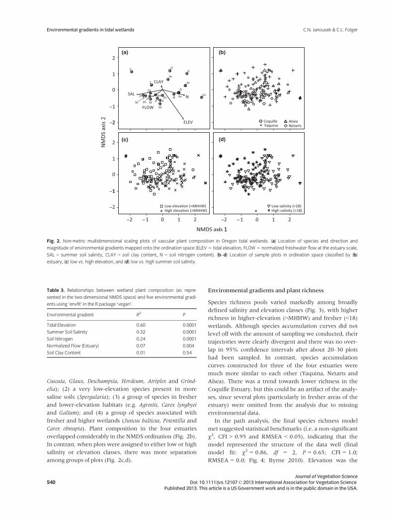
Cuscuta, Glaux, Deschampsia, Hordeum, Atriplex and Grind-

elia); (2) a very low-elevation species present in more

saline soils (Spergularia); (3) a group of species in fresher

and lower-elevation habitats (e.g. Agrostis, Carex lyngbyei

and Galium); and (4) a group of species associated with

fresher and higher wetlands (Juncus balticus, Potentilla and

Carex obnupta). Plant composition in the four estuaries

overlapped considerably in the NMDS ordination (Fig. 2b).

In contrast, when plots were assigned to either low or high

salinity or elevation classes, there was more separation

among groups of plots (Fig. 2c,d).

Environmental gradients and plant richness

Species richness pools varied markedly among broadly

defined salinity and elevation classes (Fig. 3), with higher

richness in higher-elevation (>MHHW) and fresher (<18)wetlands. Although species accumulation curves did not

level off with the amount of sampling we conducted, their

trajectories were clearly divergent and there was no over-

lap in 95% confidence intervals after about 20–30 plots

had been sampled. In contrast, species accumulation

curves constructed for three of the four estuaries were

much more similar to each other (Yaquina, Netarts and

Alsea). There was a trend towards lower richness in the

Coquille Estuary, but this could be an artifact of the analy-

ses, since several plots (particularly in fresher areas of the

estuary) were omitted from the analysis due to missing

environmental data.

In the path analysis, the final species richness model

met suggested statistical benchmarks (i.e. a non-significant

v2, CFI > 0.95 and RMSEA < 0.05), indicating that the

model represented the structure of the data well (final

model fit: v2 = 0.86, df = 2, P = 0.65; CFI = 1.0;

RMSEA = 0.0; Fig. 4; Byrne 2010). Elevation was the

Table 3. Relationships between wetland plant composition (as repre-

sented in the two-dimensional NMDS space) and five environmental gradi-

ents using ‘envfit’ in the R package ‘vegan’.

Environmental gradient R2 P

Tidal Elevation 0.60 0.0001

Summer Soil Salinity 0.32 0.0001

Soil Nitrogen 0.24 0.0001

Normalized Flow (Estuary) 0.07 0.004

Soil Clay Content 0.01 0.54

(a) (b)

(c) (d)

Fig. 2. Non-metric multidimensional scaling plots of vascular plant composition in Oregon tidal wetlands. (a) Location of species and direction and

magnitude of environmental gradients mapped onto the ordination space (ELEV = tidal elevation, FLOW = normalized freshwater flow at the estuary scale,

SAL = summer soil salinity, CLAY = soil clay content, N = soil nitrogen content). (b–d) Location of sample plots in ordination space classified by (b)

estuary, (c) low vs. high elevation, and (d) low vs. high summer soil salinity.




strongest driver of plot-level species richness among the

variables retained in the final model. Richness was highest

in plots above MHHW (Fig. 5). Soil salinity and soil clay

content were also positively related to richness, but stan-

dardized path coefficients were about three times smaller

for these variables than for elevation. Soil N, although

strongly affected by elevation (e.g. Appendix S3), and estu-

arine flow were not significantly related to richness and

were dropped from the final model.

Discussion

Many abiotic factors and biological interactions among

species are known to affect plant composition and diversity

in estuarine wetlands (Engels & Jensen 2009; Keammerer

& Hacker 2013). Gradients of salinity, elevation and other

edaphic variables may co-occur in complex patterns

(Odum 1988). Our aim in this study was to quantify the

relative strength of relationships between major environ-

mental gradients and wetland plant composition and rich-

ness and use these results to inform projections about

future changes to tidal wetlands, particularly related to sea

level rise. Our analyses suggest that: (1) the environmental

gradients most strongly associated with plant distribution

differ to some extent among species; (2) tidal elevation is

the principal driver of aggregate assemblage composition

and diversity; and (3) hydrologic differences among estuar-

ies are generally of only secondary importance, relative to

other gradients, in shaping plant distribution and composi-

tion.

Environmental gradients and species occurrences

Soil salinity, tidal elevation and soil N content were alter-

natively the most important environmental correlates of

species occurrences for the common taxa in our study. Soil

salinity was the variable most strongly associated with the

distribution of five of the 12 most common species, all of

which were more common in more saline habitats. Wat-

son & Byrne (2009) also found that salinity was associated

with the distribution of many species across the San Fran-

cisco Estuary (positively correlated with Sarcocornia and

negatively associated with other species like Scirpus califor-

nicus). Our data cannot causally explain distribution, but

other research shows that halophytes may be limited to

more saline wetlands due to competitive displacement

(Crain et al. 2004; Engels & Jensen 2010; but see also Guo

& Pennings 2012). Occurrences of a few less common spe-

cies in our data set (Carex obnupta and Galium spp.) were

negatively related to soil salinity (Appendix S4).

0 20 40 60 800 20 40 60 800 20 40 60 80

0

10

20

30

40

50

60

Number of plots sampled

Spec

ies

rich

ness

Yaquina>MHHW

<MHHW

Coquille

Alsea

Netarts

>18 ppt

<18 ppt(a) (b) (c)

Fig. 3. Species accumulation curves for (a) each estuary in the study, (b) high vs. low tidal elevation plots, and (c) high vs. low salinity plots. Polygons show

95% confidence intervals.

Tidal elevation

Soil clay content

Soilsalinity

Soilnitrogen

Plantrichness

R2 = 0.32

Estuary normalized

-flow

–0.35 (–11.35)

0.20 (0.04)

0.19(0.08)

0.57 (3.63)

R2 = 0.12

Fig. 4. Path diagram of environmental gradient effects on vascular plant

richness. Pathways in the final model are shown in black with standardized

and non-standardized (in parentheses) coefficients. Path widths are scaled

by standardized path coefficients. Non-significant variables and pathways

are in grey (soil N was strongly correlated with tidal elevation, but this path

was not included in the final model since the N to richness path was

eliminated during model selection).



Tidal elevation was the dominant environmental driver

for only a few common species we tested, including Atri-

plex and Hordeum. However, although not the single most

important gradient, elevation was also relatively strongly

related to the distribution of Potentilla, Deschampsia and

Grindelia. All five of these species tend to prefer higher

marshland. Very little variation in the distribution of Jau-

mea, Triglochin or Agrostis was explained by tidal elevation.

However, the relative importance of elevation on the

occurrence of Sarcocornia, Distichlis, Jaumea, Agrostis, Grind-

elia, and particularly Triglochin, Glaux and Plantago, might

have been underestimated since these species might have

some degree of unimodal relationships with elevation,

while hierarchical partitioning requires linear relationships

between predictor and independent variables (Heikkinen

et al. 2005).Agrostis occurred across a broad range of eleva-

tions, suggesting that it is tolerant of wide variation in

flooding intensity.

The distribution of a few species was correlated princi-

pally with other environmental gradients. For instance,

Juncus balticus had a strong affinity for N-rich soils. Tjepk-

ema & Evans (1976) observed N fixation associated with

this species in an estuary in northern Oregon - a potential

cause of this association. Davy et al. (2011) found that ele-

vation, soil redox conditions, and soil salinity have differ-

ent magnitudes of effect on species cover or occurrence in

a restored salt marsh in England, depending on the species

under consideration.

Environmental gradients and plant composition and

richness

While various environmental variables were most strongly

correlated with individual species distributions, tidal eleva-

tion appeared to be the dominant driver of overall plant

composition and plot-level richness. Tidal elevation was

the strongest correlate of plant composition in the NMDS

ordination (Table 3) and of species richness in the path

analysis (Figs 4 and 5). Tidal elevation itself is tightly cou-

pled to a variety of environmental variables, including

flooding frequency and duration and soil redox potential

(Davy et al. 2011). Increased submergence at lower eleva-

tions is known to negatively affect many wetland species,

potentially limiting diversity in these wetlands (Grace &

Pugesek 1997). Elevation was also related to other envi-

ronmental gradients such as soil N content (Fig. 4, Appen-

dix S3). In the path analysis, elevation affected plant

richness both through a strong direct effect and an indirect

effect via soil salinity.

We found maximum plant richness at elevations above

MHHW and much lower richness in frequently flooded

plots. Salinity and elevation have both been considered as

limiting plant richness in tidal wetland ecosystems (Odum

1988; Gough et al. 1994; Engels & Jensen 2009) by reduc-

ing the pool of species tolerant to salinity or flooding stress

(Grace & Pugesek 1997). Our results are consistent with

studies that show a positive relationship between plant

richness and tidal elevation (Gough et al. 1994; Grace &

Pugesek 1997; Kunza & Pennings 2008; Engels & Jensen

2009; Moeslund et al. 2011).

Soil salinity had a weak positive relationship with plot-

level plant richness in the path analysis, in contrast to

other research showing that fresher wetlands are more

diverse (Garc�ıa et al. 1993; Gough et al. 1994; Grace &

Pugesek 1997; Engels & Jensen 2009; Sharpe & Baldwin

2009; Watson & Byrne 2009;Wiezski et al. 2010). In simple

regression, plant richness was neither significantly related

to summer salinity nor to winter salinity measured in the

following season at the same plots (data not shown). Weil-

hoefer et al. (2013) also only found a weak negative salin-

ity–diversity relationship in the Oregon estuarine marsh

flora. While our species accumulation results show that

fresher wetlands do have a larger overall species pool, plot-

level richness did not differ between fresher and more

–1.0 –0.5 0.0 0.5 1.0 0 10 20 30 40 0 5 10 15 20 25 30

12

10

8

6

4

2

0

Elevation above MHHW (m) Soil salinity (ppt) Sediment clay content (%)

Plan

t ric

hnes

s

Fig. 5. Relationships between species richness and elevation, summer soil salinity and soil clay content. Plot symbols differ by estuary as in Fig 2b.




saline assemblages. Higher beta diversity in fresher wet-

lands may explain this discrepancy: assemblages in more

saline habitats can have high richness, but show little

variation in composition from plot-to-plot, whereas assem-

blages in fresher wetlands may differ more composition-

ally. In summary, salinity appears to have a relatively

strong effect on composition across Oregon estuaries (e.g.

Weilhoefer et al. 2013) and on landscape-scale diversity,

but not on plot-level richness.

Estuary-scale variation in hydrology

Our results suggest that hydrologic differences among estu-

aries play only a secondary role in structuring plant abun-

dance, composition or species richness. Some rarer species

in our data set were found in only one or a few estuaries,

but common taxa were usually present in all estuaries,

regardless of hydrologic condition (the absence of Grindelia

in Coquille is a notable exception). While hydrology may

be expected to greatly impact salinity regimes for lower-

elevation estuarine habitats such as seagrass beds, high

tidal wetlands may be relatively less impacted by variation

in the degree of river dominance because they are rarely

flooded. Groundwater inputs or precipitation may be com-

paratively more important determinants of salinity. For

instance, even during the summer in Netarts Bay (a site

expected overall to be very saline), wetlands at very high

tidal elevations had surprisingly low salinities, perhaps due

to groundwater inputs or retention of spring precipitation.

Plant composition, such as the presence of a large swath of

salt-intolerant Carex obnuptamarsh at the estuarine–upland

margin, reflected these edaphic conditions. Conversely,

many low-marsh plots in the river-dominated Coquille

estuary resembled low marshes in the other estuaries pop-

ulated by succulent halophytes, probably because they

experience frequent tidal inundation and are situated geo-

graphically close to themouth of the estuary.

While our results suggest that watershed-level hydrol-

ogy may not be a major driver of plant composition in Ore-

gon tidal wetlands, additional data are needed on linkages

between watershed hydrology and overall wetland species

richness and composition. In a study of the deltas of 17

estuaries in the Puget Sound region of Washington and

British Columbia, Hutchinson (1988) found a fairly high

degree of correspondence between marsh assemblages and

estuary-level environmental metrics (e.g. river discharge/

near-shore wave power). He suggested that salinity differ-

ences among estuaries drive these patterns, with fresher

estuaries having increased dominance of species such as

Carex lyngbyei, Triglochin and Schoenoplectus americanus, and

more saline estuaries having higher abundance of Sarcocor-

nia, Distichlis, Juncus balticus and Potentilla. Few other stud-

ies appear to examine relationships between wetland plant

composition and estuarine hydrology at regional scales.

Sharpe & Baldwin (2009) found that plant composition

varied more among wetlands from different salinity

regimes that were located relatively close geographically

than between wetlands of similar salinity classes located

on opposite sides of the Chesapeake Bay estuary. Kunza &

Pennings (2008) suggested that higher diversity in Texas

vs. Georgia salt marshes may be due to differences in tidal

regimes.

Implications for climate change

Future coastal wetlands are likely to experience a suite of

environmental changes, including higher temperatures,

elevated CO2, sea level rise and changes in estuarine

hydrology (Parker et al. 2011). Our data on vegetation

relationships with some of these gradients suggess that

plant composition may be particularly sensitive to changes

in relative flooding intensity in estuarine marshes. Modest

degrees of relative SLR may have a large effect on species

composition and diversity by changing flooding regimes

and soil biogeochemistry (Baldwin et al. 2001). Sea level

rise modelling by Moeslund et al. (2011) and Stralberg

et al. (2011) suggests that higher tidal wetlands may be

particularly vulnerable. Sea level rise may also result in

higher salinities in wetland soils in more inland regions of

estuaries (Callaway et al. 2007). Changes in the timing of

coastal precipitation, such as intensified seasonality, may

also change salinity, although changes in snowfall-to-pre-

cipitation ratios are unlikely to impact salinity because

snowfall is not a major source of freshwater in the Oregon

coast range. Elevated salinity may have secondary effects

on composition by favouring halophytes such as Sarcocor-

nia, Distichlis, Grindelia and Jaumea at the expense of less

salt-tolerant species.

Future SLR is dependent on multiple factors that cannot

yet be accurately projected. Local sediment supply, in situ

organic matter production or sediment compaction, and

global SLR (itself affected by future rates of anthropogenic

CO2 emissions, ice sheet melting, etc.), are all important

components for projecting the futuremagnitude of relative

SLR. Despite these uncertainties, if wetland accretion rates

cannot match relative SLR, the direction of climate change

effects on estuaries is clear: flooding and salinity stresses on

plants will increase. Our data suggest that increasing these

factors will change plant composition and lower vascular

plant richness.

Conclusions

Plant composition and richness varied across a suite of

environmental gradients in the studied wetlands. Relative

gradient importance depended in part on which metrics of



plant composition were under investigation, but elevation

and salinity consistently emerged as important drivers of

vegetation structure. To the extent that future SLR

increases submergence times and salinity exposure in Paci-

fic Northwest tidal marshes and swamps, our results sug-

gest that vegetation composition will change and wetland

plant richness will decline. Altered vegetation structure in

these important coastal ecosystems may in turn lead to

changes in ecosystem function.

Acknowledgements

We thank D. Beugli, H. Brunner, V. Goldsmith, J. Saari-

nen, K. Marko, J. Stecher, T. Ernst, M. Frazier, L. Brophy,

R. Loiselle, T. MochonCollura, S. Cline and M. Armstrong

for various lab, field, technical and statistical assistance. P.

Clinton kindly provided GIS support. B. Watson, M. Fra-

zier, R. Halvorsen and two anonymous reviewers made

helpful comments on the manuscript. Sampling was made

possible by the cooperation of numerous landholders

including the US Fish andWildlife Service (Bandon NWR),

BLM, US Forest Service, Oregon State Parks, Oregon State

University, Port of Toledo, Port of Bandon, The Wetlands

Conservancy, van Eck Foundation and other private own-

ers. The information in this publication has been funded

by the U.S. Environmental Protection Agency. It has been

subjected to review by the National Health and Environ-

mental Effects Research Lab and approved for publication.

Approval does not signify that the contents reflect the

views of the Agency, nor does mention of trade names or

commercial products constitute endorsement or recom-

mendation for use.

References

Arnold, S.J. 1972. Species densities of predators and their prey.

The American Naturalist 106: 220–236.

Baldwin, A.H., Egnotovich, M.S. & Clarke, E. 2001. Hydrologic

change and vegetation of tidal freshwater marshes: field,

greenhouse, and seed-bank experiments. Wetlands 21:

519–531.

Barbier, E.B., Hacker, S.D., Kennedy, C., Koch, E.W., Stier, A.C.

& Silliman, B.R. 2011. The value of estuarine and coastal

ecosystem services. Ecological Monographs 81: 169–193.

Byrne, B.M. 2010. Structural equation modeling with AMOS, 2nd

edn. 396 pp. Routledge, New York, NY, US.

Callaway, J.C., Parker, V.T., Vasey, M.C. & Schile, L.M. 2007.

Emerging issues for the restoration of tidal marsh ecosystems

in the context of predicted climate change. Madro~no 54:

234–248.

Chevan, A. & Sutherland, M. 1991. Hierarchical partitioning.

The American Statistician 45: 90–96.

Cowardin, L.M., Carter, V., Golet, F.C. & LaRoe, E.T. 1979. Classi-

fication of wetlands and deepwater habitats of the United States. US

Fish and Wildlife Publication FWS/BSB-79/31, Washington,

DC, US.

Crain, C.M., Silliman, B.R., Bertness, S.L. & Bertness, M.D.

2004. Physical and biotic drivers of plant distribution across

estuarine salinity gradients. Ecology 85: 2539–2549.

Cui, B.-S., He, Q. & An, Y. 2011. Community structure and abi-

otic determinants of salt marsh plant zonation vary across

topographic gradients. Estuaries and Coasts 34: 459–469.

Davy, A.J., Brown, M.J.H., Mossman, H.L. & Grant, A. 2011.

Colonization of a newly developing salt marsh: disentangling

independent effects of elevation and redox potential on halo-

phytes. Journal of Ecology 99: 1350–1357.

Eilers, H.P. 1975. Plants, plant communities, net production and tide

levels: the ecological biogeography of the Nehalem salt marshes, Til-

lamook County, Oregon. Ph.D. thesis, Oregon State University,

Corvallis, OR, US.

Engels, J.G. & Jensen, K. 2009. Patterns of wetland plant diver-

sity along estuarine stress gradients of the Elbe (Germany)

and Connecticut (USA) rivers. Plant Ecology and Diversity 2:

301–311.

Engels, J.G. & Jensen, K. 2010. Role of biotic interactions and

physical factors in determining the distribution of marsh

species along an estuarine salinity gradient. Oikos 119:

679–685.

Engle, V.D. 2011. Estimating the provision of ecosystem services

by Gulf ofMexico coastal wetlands.Wetlands 31: 179–193.

Garc�ıa, L.V., Mara~n�on, T., Moreno, A. & Clemente, L. 1993.

Above-ground biomass and species richness in a Mediterra-

nean salt marsh. Journal of Vegetation Science 4: 417–424.

Gedan, K.B., Crain, C.M. & Bertness, M.D. 2009. Small-mammal

herbivore control of secondary succession in New England

tidal marshes. Ecology 90: 430–440.

Gough, L., Grace, J.B. & Taylor, K.L. 1994. The relationship

between species richness and community biomass: the

importance of environmental variables.Oikos 70: 271–279.

Grace, J.B. & Pugesek, B.H. 1997. A structural equation model of

plant species richness and its application to a coastal wetland.

American Naturalist 149: 436–460.

Guo, H. & Pennings, S.C. 2012. Mechanismsmediating plant dis-

tributions across estuarine landscapes in a low-latitude tidal

estuary. Ecology 93: 90–100.

Heikkinen, R.K., Luoto, M., Kuussaari, M. & P€oyry, J. 2005.

New insights into butterfly–environment relationships using

partitioning methods. Proceedings of the Royal Society, Series B

272: 2203–2210.

Hutchinson, I. 1988. The biogeography of the coastal wetlands of

the Puget Trough: deltaic form, environment, and marsh

community structure. Journal of Biogeography 15: 729–745.

Jefferson, C.A. 1975. Plant communities and succession in Oregon

coastal salt marshes. PhD dissertation, Oregon State University,

Corvallis, OR, US.

Keammerer, H.B. & Hacker, S.D. 2013. Negative and neutral

marsh plant interactions dominate in early life stages and

across physical gradients in an Oregon estuary. Plant Ecology

214: 303–315.




Kruskal, J.B. 1964a. Multidimensional scaling by optimizing

goodness of fit to a nonmetric hypothesis. Psychometrika 29:

1–27.

Kruskal, J.B. 1964b. Nonmetric multidimensional scaling: a

numerical method. Psychometrika 29: 115–129.

Kunza, A.E. & Pennings, S.C. 2008. Patterns of plant diversity in

Georgia and Texas salt marshes. Estuaries and Coasts 31: 673–

681.

Lee, H. II & Brown, C.A. (eds.) 2009. Classification of regional pat-

terns of environmental drivers and benthic habitats in Pacific

Northwest estuaries. US EPA, Office of Research and Develop-

ment, Newport, OR, US.

Liverman, M.C. 1981. Multivariate analysis of a tidal marsh ecosys-

tem at Netarts Spit, Tillamook County, Oregon. MS Thesis Oregon

State University, Corvallis, OR, US.

Moeslund, J.E., Arge, L., Bøcher, P.K., Nygaard, B. & Svenning,

J.-C. 2011. Geographically comprehensive assessment of

salt–meadow vegetation–elevation relations using LiDAR.

Wetlands 31: 471–482.

National Oceanic and Atmospheric Administration. 2003. Com-

putational techniques for tidal datums handbook. NOAA Special

Publication NOS CO-OPS 2, US Department of Commerce,

Silver Spring, MD, US.

Odum, W.E. 1988. Comparative ecology of tidal freshwater and

salt marshes.Annual Review of Ecology and Systematics 19: 147–

176.

Økland, R.H. 1996. Are ordination and constrained ordination

alternative or complementary strategies in general ecological

studies? Journal of Vegetation Science 7: 289–292.

Parker, V.T., Callaway, J.C., Schile, L.M., Vasey, M.C. & Herbert,

E.R. 2011. Climate change and San Francisco Bay-Delta tidal

wetlands. San Francisco Estuary andWatershed Science 9: 1–15.

Pennings, S.C., Selig, E.R., Houser, L.T. & Bertness, M.D. 2003.

Geographic variation in positive and negative interactions

among salt marsh plants. Ecology 84: 1527–1538.

Pennings, S.C., Grant, M.-B. & Bertness, M.D. 2005. Plant zona-

tion in low-latitude salt marshes: disentangling the roles of

flooding, salinity and competition. Journal of Ecology 93: 159–

167.

Rand, T.A. 2000. Seed dispersal, habitat suitability and the distri-

bution of halophytes across a salt marsh tidal gradient. Jour-

nal of Ecology 88: 608–621.

Sharpe, P.J. & Baldwin, A.H. 2009. Patterns of wetland plant spe-

cies richness across estuarine gradients of Chesapeake Bay.

Wetlands 29: 225–235.

Silvestri, S., Defina, A. & Marani, M. 2005. Tidal regime, salinity

and salt marsh plant zonation. Estuarine Coastal Shelf Science

62: 119–130.

Stralberg, D., Brennan, M., Callaway, J.C., Wood, J.K., Schile,

L.M., Jongsomjit, D., Kelly, M., Parker, V.T. & Crooks, S.

2011. Evaluating tidal marsh sustainability in the face of sea-

level rise: a hybrid modeling approach applied to San Fran-

cisco Bay. PLoS One 6: e27388.

Tjepkema, J.D. & Evans, H.J. 1976. Nitrogen fixation associated

with Juncus balticus and other plants of Oregon wetlands. Soil

Biology and Biochemistry 8: 505–509.

Watson, E.B. & Byrne, R. 2009. Abundance and diversity of tidal

marsh plants along the salinity gradient of the San Francisco

Estuary: implications for global change ecology. Plant Ecology

205: 113–128.

Weilhoefer, C.L., Nelson, W.G., Clinton, P. & Beugli, D.M. 2013.

Environmental determinants of emergent macrophyte vege-

tation in Pacific Northwest estuarine tidal wetlands. Estuaries

and Coasts 36: 377–389.

Wiezski, K., Guo, H., Craft, C.B. & Pennings, S.C. 2010. Ecosys-

tem functions of tidal fresh, brackish, and salt marshes on

the Georgia coasts. Estuaries and Coasts 33: 161–169.

Zedler, J.B. 2010. How frequent storms affect wetland vegeta-

tion: a preview of climate-change impacts. Frontiers in Ecology

and the Environment 8: 540–547.

Zedler, J.B., Callaway, J.C., Desmond, J.S., Vivian-Smith, G.,

Williams, G.D., Sullivan, G., Brewster, A.E. & Bradshaw,

B.K. 1999. California salt-marsh vegetation: an improved

model of spatial pattern. Ecosystems 2: 19–35.

Supporting Information

Additional Supporting Information may be found in the

online version of this article:

Appendix S1. Floristic and natural history references

used in the study.

Appendix S2. Relationships between soil N, soil clay

content, PAR transmission, tidal elevation and soil salinity.

Appendix S3. Percent variation in minor species’

occurrence accounted for by five environmental gradients

in hierarchical partitioning of multivariate logistic regres-

sion models (Elev, elevation; Sal, soil salinity; Flow, estua-

rine flow; Clay, percent clay content of sediment; N, total

organic nitrogen).

Appendix S4. List of species, by estuary, located

inside 0.25m2 plots in the study



Date post:	23-Dec-2016
Category:	Documents
Upload:	rune
View:	212 times
Download:	0 times

Variation in tidal wetland plant diversity and composition within and among coastal estuaries:...

Documents