Variational data assimilation experiments at NCEP using ocean surface winds and sea surface temperatures data Tsann-wang Yu Environmental Modeling Center National Centers for Environmental Prediction National Weather Service, NOAA Washington, D. C., 20233
Transcript
Variational data assimilation experiments at NCEP using ocean surface winds and sea
surface temperatures data
Tsann-wang Yu
Environmental Modeling Center
National Centers for Environmental Prediction
National Weather Service, NOAA
Washington, D. C., 20233
Outline
• Current status of NWP operations at NCEP
• Data assimilation and development strategies for ocean and atmospheric
• Use of QuikSCat winds and GOES and AVHRR data assimilation experiments
• Current developments in data assimilation at NCEP / JCSDA
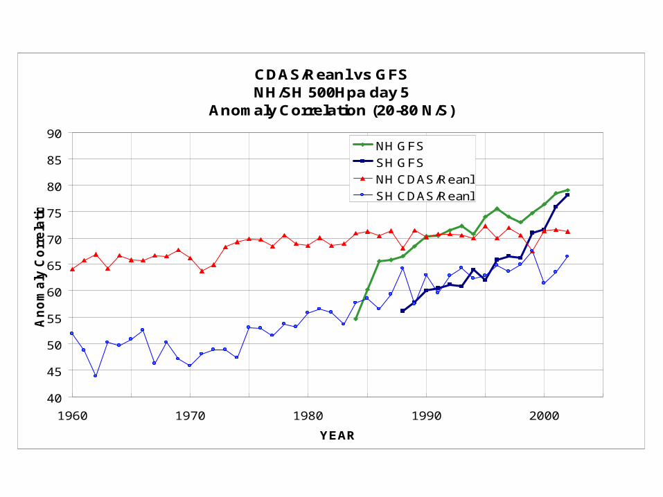
Evolution of forecast skill for the northern and southern hemispheres
CDAS/Reanl vs GFSNH/SH 500Hpa day 5
Anomaly Correlation (20-80 N/S)
40
45
50
55
60
65
70
75
80
85
90
1960 1970 1980 1990 2000
YEAR
An
om
aly
Co
rre
lati
on
NH GFS
SH GFS
NH CDAS/Reanl
SH CDAS/Reanl
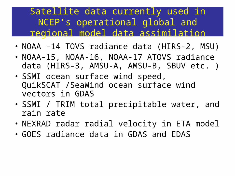
Satellite data currently used in NCEP’s operational global and regional model data assimilation
• SSMI / TRIM total precipitable water, and rain rate
• NEXRAD radar radial velocity in ETA model• GOES radiance data in GDAS and EDAS
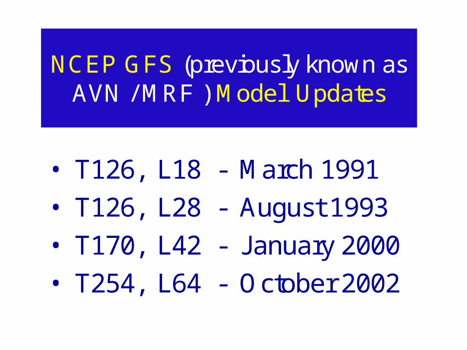
NCEP GFS (previously known as AVN / MRF ) Model Updates
• T126, L18 - March 1991
• T126, L28 - August 1993
• T170, L42 - January 2000
• T254, L64 - October 2002
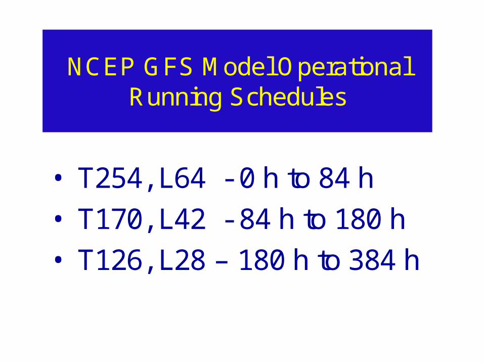
NCEP GFS Model Operational Running Schedules
• T254, L64 - 0 h to 84 h
• T170, L42 - 84 h to 180 h
• T126, L28 – 180 h to 384 h
Data Assimilation
t1
t3
Analysis pdfFor the Grid
Forecast pdf For the Grid
Initial Condition:Analysis Mean
Observation pdf
t2
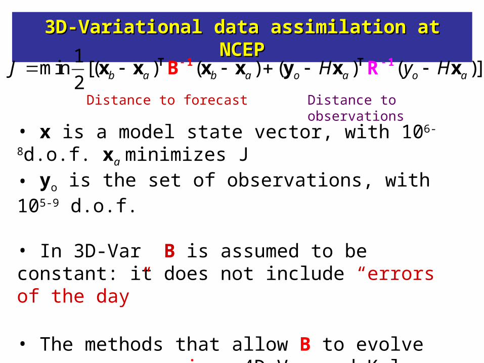
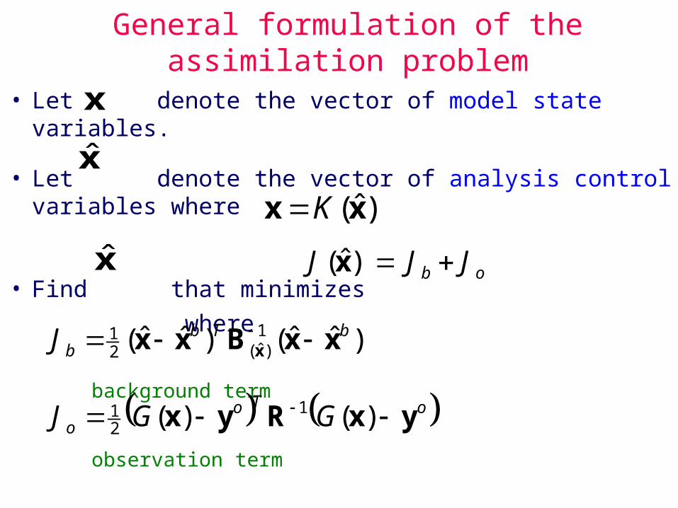
3D-Variational data assimilation at NCEP3D-Variational data assimilation at NCEP
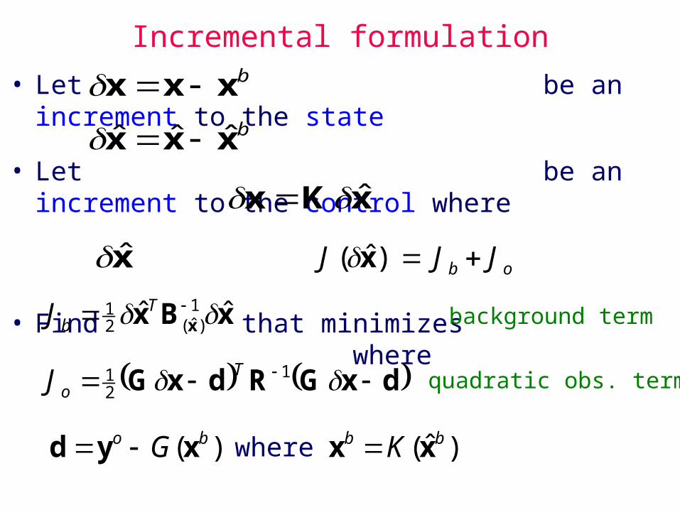
1min [( ) ( ) ( ) ( )]
2 b a b a o a o aJ H y H 1T T 1x x Rx y x xB x
• x is a model state vector, with 106-8d.o.f. xa minimizes J• yo is the set of observations, with 105-9 d.o.f.
• In 3D-Var B is assumed to be constant: it does not include “errors of the day”
• The methods that allow B to evolve are very expensive: 4D-Var and Kalman Filtering, and require the linear tangent and adjoint models.
Distance to forecast Distance to observations
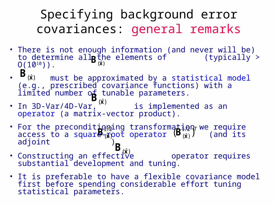
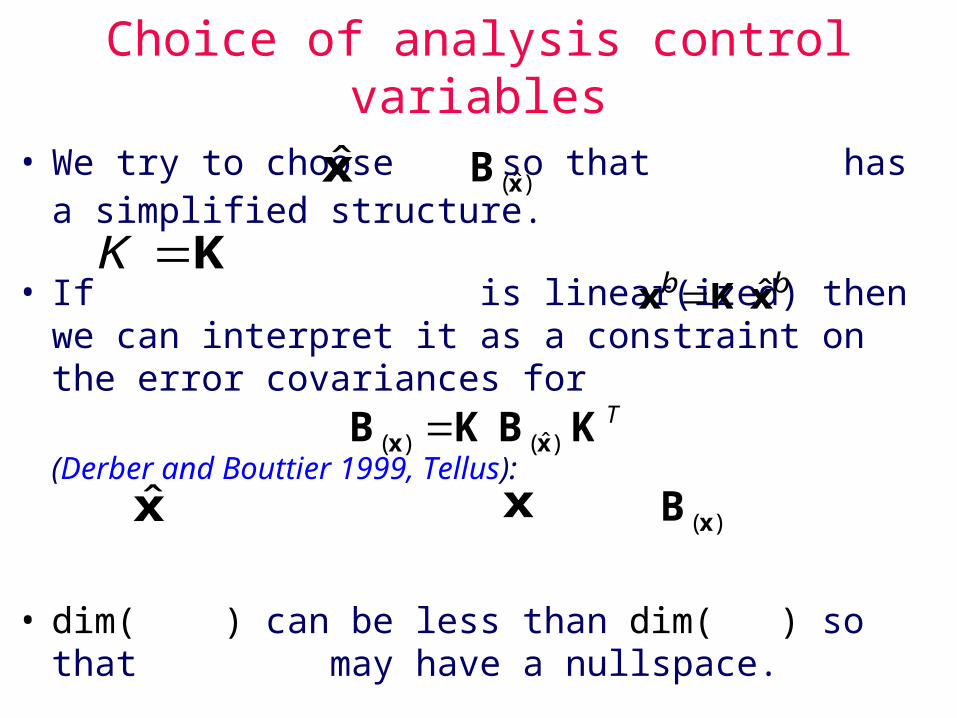
Specifying background error covariances: general remarks
• There is not enough information (and never will be) to determine all the elements of (typically > O(1010)).
• must be approximated by a statistical model (e.g., prescribed covariance functions) with a limited number of tunable parameters.
• In 3D-Var/4D-Var, is implemented as an operator (a matrix-vector product).
• For the preconditioning transformation we require access to a square-root operator (and its adjoint ).
• Constructing an effective operator requires substantial development and tuning.
• It is preferable to have a flexible covariance model first before spending considerable effort tuning statistical parameters.
)ˆ(xB
)ˆ(xB
)ˆ(xB
2/1)ˆ(xB T)( 2/1
)ˆ(xB
)ˆ(xB
• Ocean observations are relatively sparse so it is difficult to estimate background error statistics from innovations. Considerable spatial and temporal averaging is required (e.g., Martin et al. 2002).
• With few observations the role of is critical for exploiting available data-sets effectively (e.g., surface altimeter data).
• Added complexity due to the presence of continental boundaries (boundary conditions, scales, spectra, balance).
• Rich variety of scales: mesoscale (Gulf Stream, Kuroshio regions) ~O(10km) and synoptic scale (tropics) ~ O(100km).
)(xB
Specifying background error covariances: specific remarks for the ocean
Ocean surface winds and sea surface temperatures are two of the most important fields responsible for
• Physical coupling of ocean and atmosphere - air sea interaction.
• Directly driving ocean waves and current circulations – ocean general circulations.
• Affecting accuracy of numerical weather and climate forecasts.
Data assimilation experiments to test QuikSCAT winds
and AVHRR and GOES infra-red radiance SST data
Conventional data Assimilation
CNTL
SCAT Winds, or SST + Conventional
data Assimilation
TEST
Effect of SCAT Winds ( TEST – CNTL)
Observing System Experiments (OSE) to test Quikscat winds and infra-red sea surface temperatures data from
AVHRR and GOES
Impact of SCAT winds or SST = (TEST –CNTL)
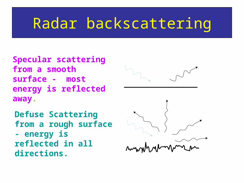
Radar backscattering
Specular scattering from a smooth surface - most energy is reflected away.
Defuse Scattering from a rough surface - energy is reflected in all directions.
Bragg scattering
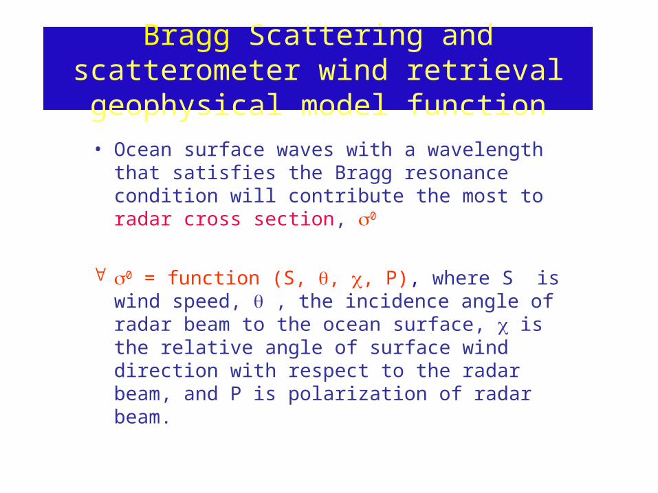
Bragg Scattering and scatterometer wind retrieval geophysical model function
• Ocean surface waves with a wavelength that satisfies the Bragg resonance condition will contribute the most to radar cross section, 0
0 = function (S, , , P), where S is wind speed, , the incidence angle of radar beam to the ocean surface, is the relative angle of surface wind direction with respect to the radar beam, and P is polarization of radar beam.
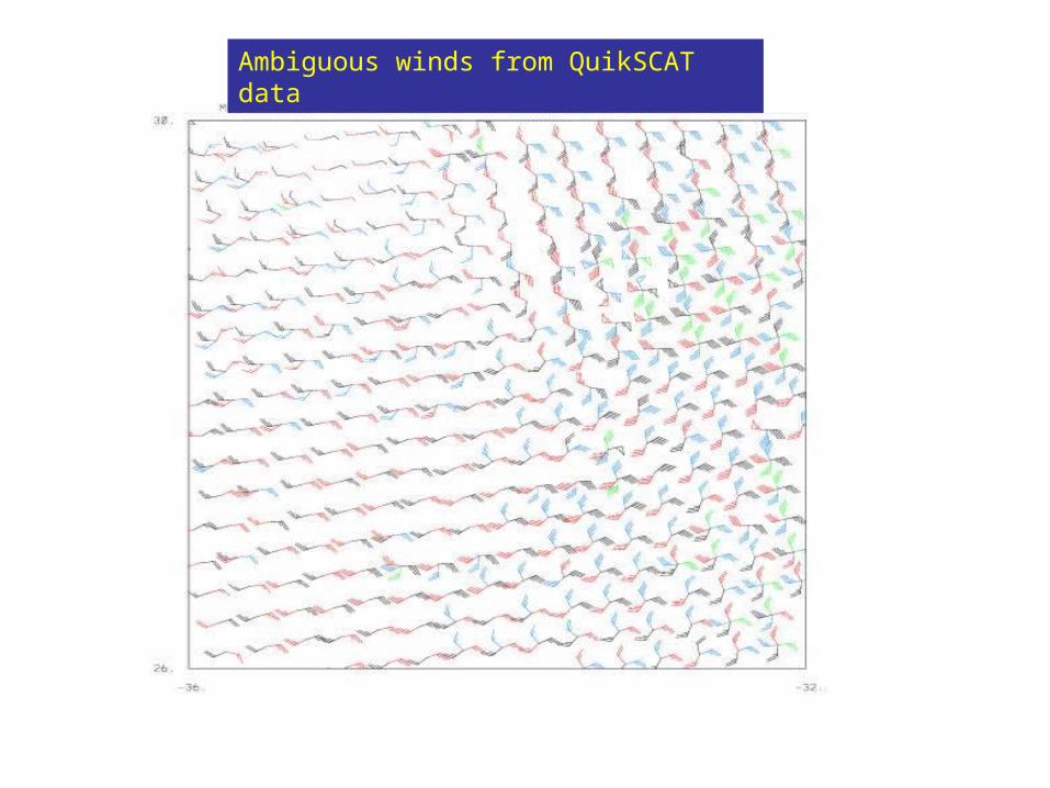
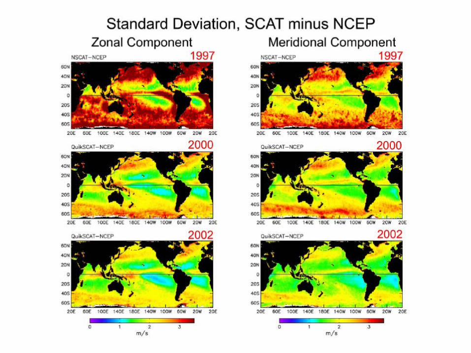
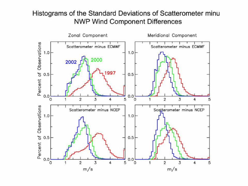
Characteristics of QuikSCATwinds - NASA SeaWind satellite
• Spatial resolution of 25 km, with a satellite swath of 1800 km
• Ambiguity problem in wind direction ( up to 4 wind directions)
QuikSCAT winds – introduced into Ocean Prediction Center operational workstations in the fall of 2001 – are now fully
integrated into the warning & forecast decision process
----
Wind Speed (Knots): 65 50 35 30 25 20
QuikSCAT Winds1800 UTC 17 Feb 03
NCEP GFS 40m Winds - 6 hr FCST 1800 UTC 17 Feb 03
QuikSCAT winds – a numerical model diagnostic
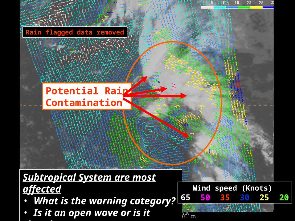
Rain flagged data removed
Potential RainContamination
Subtropical System are most affected• What is the warning category? • Is it an open wave or is it closed? • If closed, where is the center?
Wind speed (Knots) 65 50 35 30 25 20
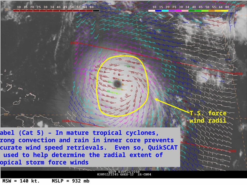
MSW = 140 kt. MSLP = 932 mb
Isabel (Cat 5) – In mature tropical cyclones,strong convection and rain in inner core prevents accurate wind speed retrievals. Even so, QuikSCATis used to help determine the radial extent of tropical storm force winds
T.S. forcewind radii
Hurricane Force Extratropical Cyclone48.5N 26.89W
Hurricane Force Winds
QuikSCAT pass from 06NOV 0630UTC
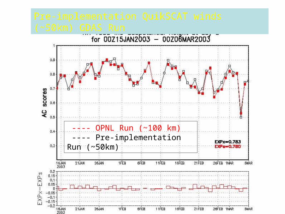
Summary of Results of GDAS experiment Using 100 km resolution QuikSCAT winds at NCEP
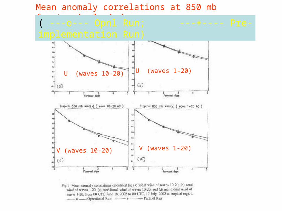
Summary of GDAS experiment Using 50 km resolution QuikSCAT winds at NCEP
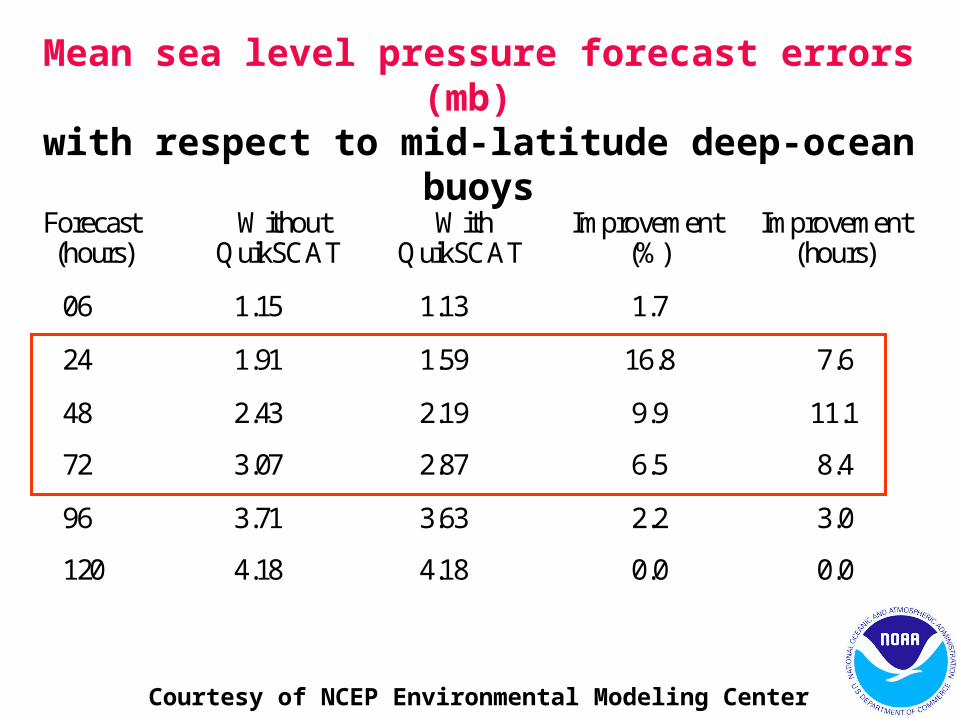
NCEP Operational GDAS – T254, L64 Assimilation Exp. – January 8, 2003 to
March 8, 2003 (60 days) Found positive impact on heights and
winds at all levels for both N.H. and S.H., especially for winds over the tropical oceans
QuikSCAT winds (50 km) – were implemented at NCEP GDAS on March 11, 2003
35
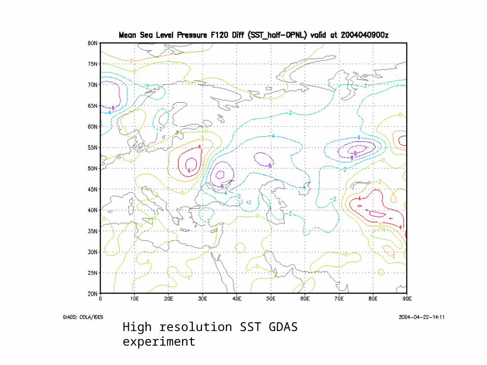
Global data assimilation experiments using high resolution SST analyses at NCEP
(Yu, 2004)
• Motivation : ECMWF has already used NCEP high resolution SST analysis in NWP operation; high resolution SST are already used in NCEP EDAS operation
• Purpose: To investigate the impact of high resolution SST on NCEP GDAS and NWP forecasts for possible implementation
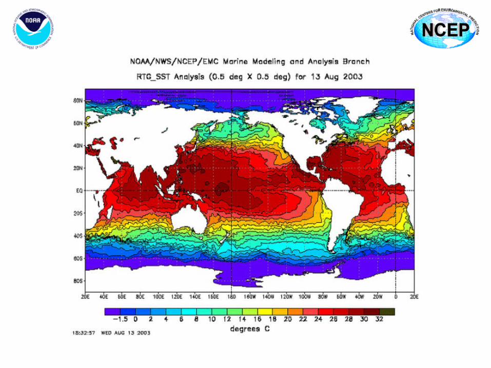
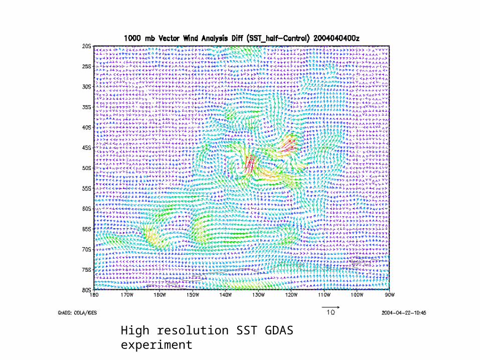
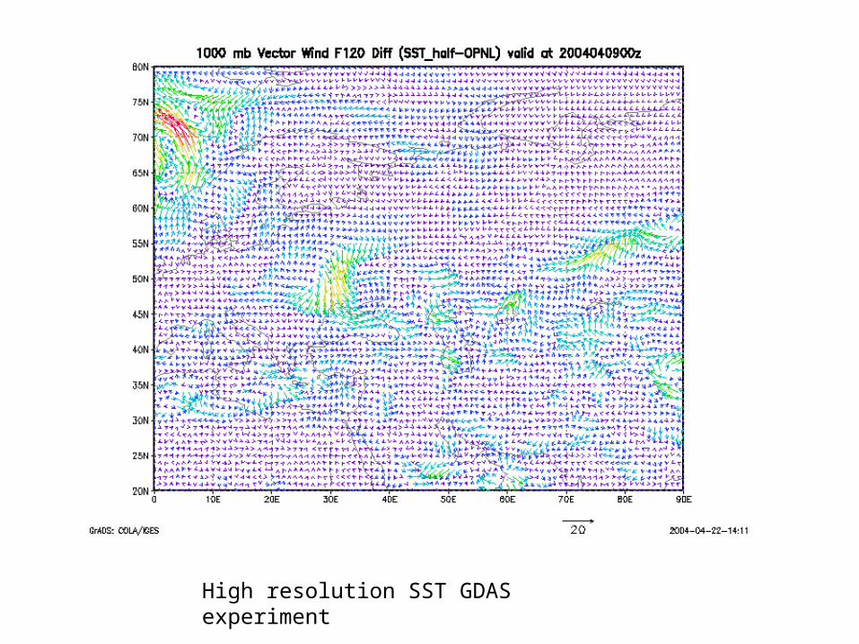
High resolution SST GDAS experiments
High resolution SST GDAS experiment
High resolution SST GDAS experiment
High resolution SST GDAS experiment
Use of AVHRR and GOES satellite infra-red temperature data at NOAA Coastal Ocean
Forecast System ( O’Connor, Lozano, and Yu, 2004)
• Scientific objective : High resolution (about 8km) infra-red sea surface temperatures data from AVHRR and GOES should improve mesoscale features of ocean analyses
• Major findings: use of GOES’ SST in ocean data assimilation is found to lead to large improvements for depicting Gulf Stream feature
SST retrievals from GOES and AVHRR brightness temperatures
• The basic idea of MCSST came from Andingand Kauth(1970) – showed a quasi-linear relationship between radiation deficit due to atmospheric water vapor and the brightness temperature difference in two adjacent wavelength bands in the infra-red.
• An example of SST retrieval equations -
Ts = a1T4+a2(T4-T5)+a3(T4 –T5)(secz-1)+a4
Ocean Forecasting – Present (1-2 days) Prediction of SST, Gulfstream, Hurricane-Ocean Coupling, Tides and Water Levels, Boundary Conditions for Bays and Estuaries, Search & Rescue Operations, Toxic Spill Containment, Ecosystem
Management,..
Features: Primitive Equations, Forced by ETA Model Fluxes; Assimilation of SST, XBT, altimetry.
Princeton Ocean ModelDomain: East CoastVertical Coordinate: Sigma (19 levels)Horizontal Resolution: 10 km near coast to 20 km in deep oceanLateral Boundary Condition: Monthly mean values for temperatures, salinity, and transport at the open ocean boundaries and monthly mean values for river run-off at the coastal boundaries
Surface Currents
SST
Coastal Ocean Forecast System (COFS)
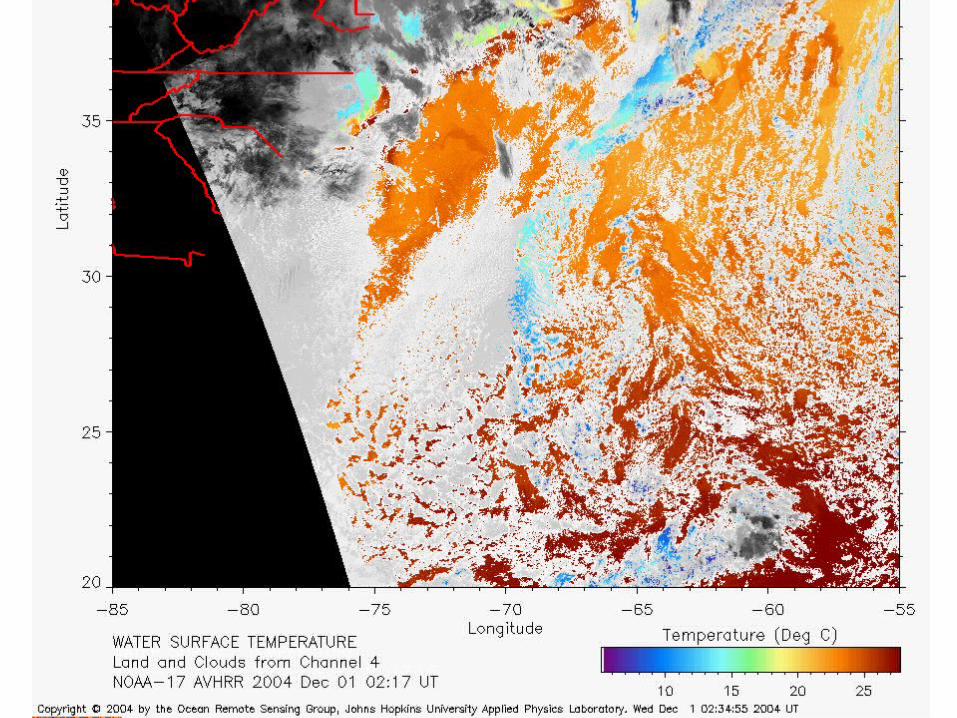
Characteristics of AVHRR and GOES infra-red temperatures
• Both AVHRR (Advanced Very High Resolution Radiometer ) and GOES (Geo-stationary Operational Environmental Satellite) are NOAA satellites using Multi-channel sea surface temperature (MCSST) equations
• Both are infra-red temperatures based retrievals and are of very high spatial resolution – AVHRR (8km), and GEOS (4 km) for NCEP operations
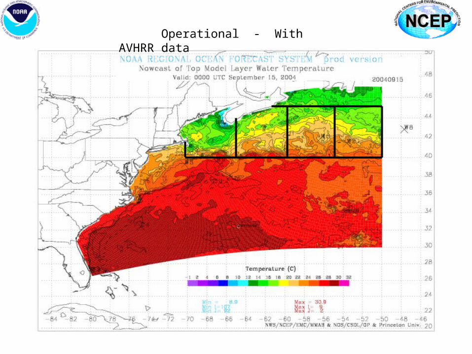
Operational - With AVHRR data
Experimental – with AVHRR and GOES data
Summary from use of GOES and AVHRR brightness temperatures in
Coastal Ocean Forecast System
• Use of GOES infra-red brightness temperature data improves Gulf stream features
• Needs to expand 2D Var Univariateanalysis to 3D multivariate analyses
Recent developments of the satellite assimilation at NCEP /JCSDA
• AQUA / AMSUR–E wind speed data and NRL’s Windsat polar-metric radiometer derived ocean surface vector winds
• GPS occultation data for global 3DVar• NOAA –15, NOAA –16, NOAA-17, AMSU
radiance, GOES, AVHRR infra-red SST and altimeter data are being tested in ocean data assimilation
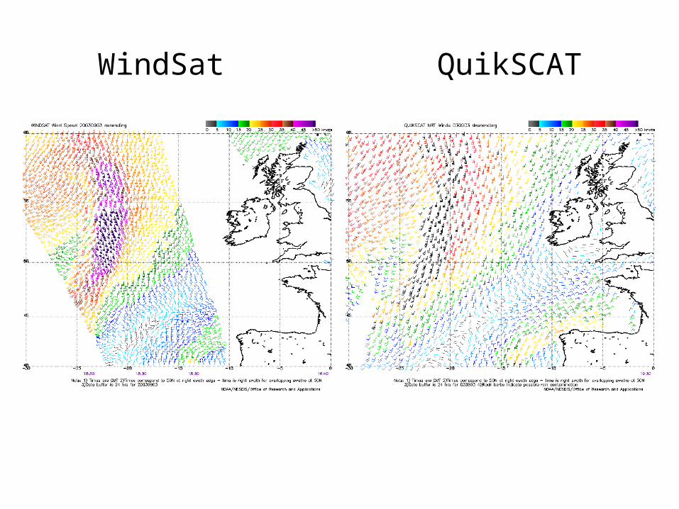
WindSat-Mission • SWindSat was
successfully launched on January 6th 2003 with the objectives to:
• Ddemonstrate the capability of Polarimetric Microwave Radiometry to measure the Ocean Surface Wind Vector from Space, and show the potential to measure other EDR’s: SST, Water Vapor, Cloud liquid water, rain rate, sea ice and snow cover.
WindSat QuikSCAT
Wind Speed from AQUA (EOS)
AMSR-E
Concluding Remarks
• Remote sensing data are important for oceanic atmospheric research and applications, and numbers of observations will continue to increase in the future.
• Data assimilation is the most scientifc approach to effectively use the remote sensing data.
• Current and near future research efforts are centered on the specification of background error covariances in the 3D-VAR and 4D-VAR variational analysis for NWP operations.
• Ensemble forecast and Kalman Filter approaches are the most active areas of research and development in the data assimilation.
Thank you very much for your attention !
• We write the matrix-vector product as
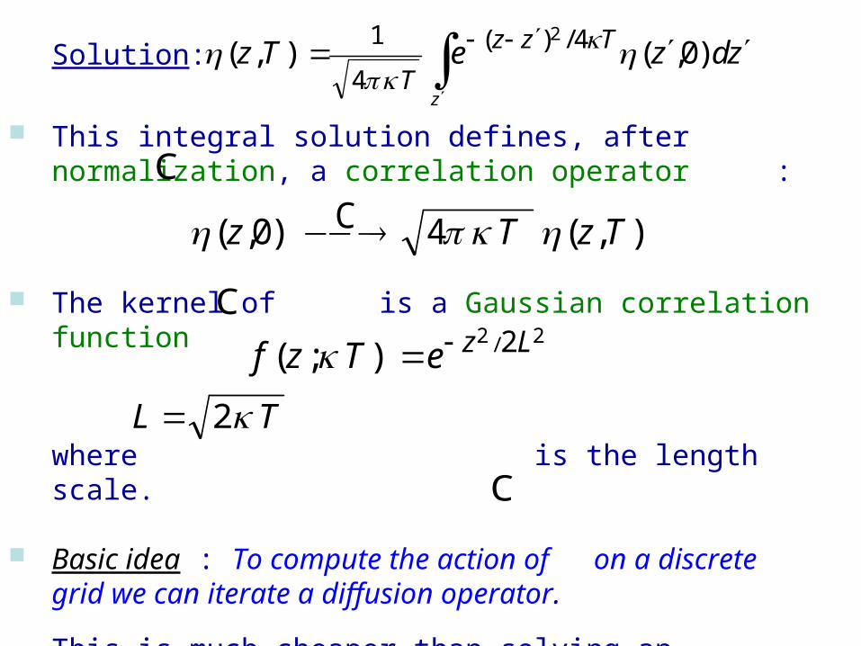
• We solve a generalized diffusion equation (GDE) to perform the smoothing action of the square-root of the correlation operator ( ).
• We multiply by the standard deviations of background ( ) error ( ).
Modelling background error covariances
vCΣvBx xxx2/1)ˆ()ˆ(
2/1)ˆ(0ˆ
bx̂
2/1)ˆ(xC
)ˆ(xΣ
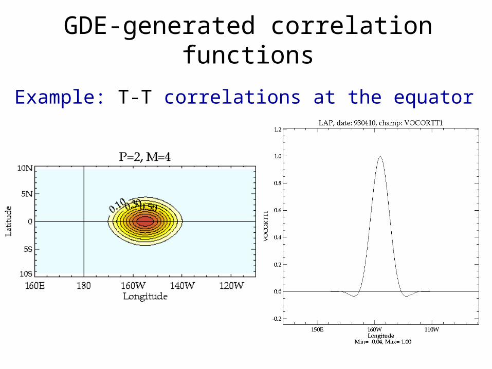
Univariate correlation modelling using a diffusion equation