33
VARIATIONAL FORMULATION OF THE STRAIN LOCALIZATION PHENOMENON GUSTAVO AYALA
| Date post: | 18-Dec-2015 |
| Category: |
Documents |
| Upload: | rodger-stokes |
| View: | 236 times |
| Download: | 0 times |

VARIATIONAL FORMULATION OF THE STRAIN LOCALIZATION
PHENOMENON
GUSTAVO AYALA

OBJECTIVE
To develop a variational formulation of the strain
localization phenomenon, its implementation in a
FE code, and its application to real problems.
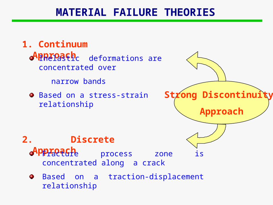
MATERIAL FAILURE THEORIES
2. Discrete Approach
1. Continuum Approach
Fracture process zone is concentrated along a crack
Based on a traction-displacement relationship
Inelastic deformations are concentrated over
narrow bands
Based on a stress-strain relationshipStrong Discontinuity
Approach

Variation of displacement, strain and stress fields
2. DISCRETE APPROACH (DA)
1. CONTINUUM APPROACH (CA)
x
x
x
x
x
x
[ u ]
u
k=0
k=0
k
[ u ]
[ u ]
= [ u ]1k
S
= [ u ]s
x
x
x
S S
Weak discontinuity
Strong discontinuity
a) b)
- n
h
n
k=0
+-
h
k=0
+
SS
-
+i-
i+
-
+
+-
k=0
n -+
k=0
S
SS
i-
i+
-+
a) b)
+- Sn
+
S- S+
--+

CA-Weak Discontinuity
in Ω Kinematical compatibility
in Ω Constitutive compatibility
in Ω Internal equilibrium
on σ External equilibrium
on Ωh Outer traction continuity
on Ωh Inner traction continuity
\
0
( ) 0
0
0
0S
S
S
u
n
n
b
t
n n =
n n
a) b)
- n
h
n
k=0
+-
h
k=0
+
SS
-
+i-
i+
-
+

CA-Strong Discontinuity
in Ω Kinematical compatibility
in Ω Constitutive compatibility
in Ω\S Internal equilibrium
on σ External equilibrium
on S Outer traction continuity
on S Inner traction continuity
\
0
( ) 0
0
0
0S
S
S
u
n
n
b
t
n n =
n n
+-
k=0
n -+
k=0
S
SS
i-
i+
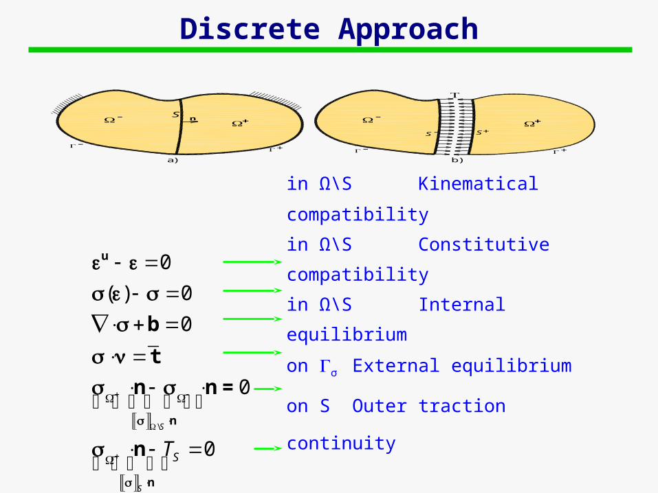
Discrete Approach
in Ω\S Kinematical compatibility
in Ω\S Constitutive compatibility
in Ω\S Internal equilibrium
on σ External equilibrium
on S Outer traction continuity
on S Inner traction continuity
\
0
( ) 0
0
0
0
u
n
n
b
t
n n =
nS
S
ST
-+
a) b)
+- Sn
+
S- S+
--+

ENERGY FUNCTIONAL BY FRAEIJS DE VEUBEKE (1951)
ENERGY FUNCTIONAL OF THE LINEAR ELASTIC PROBLEM
V u, , , t : b u t u t u uu
u W d d d
V u, , , t U P D
1: :
2W C
u
U W d
b u t uP d d
t u u :u
uD d d
t
u
b

FRAEIJS DE VEUBEKE (1951)
Through
That is
, , , 0 V u t
: : :
0u u
u d d d
v d v d d
V b u
t u t u u u t
Find the fields
, , , , , ,t t t and tu x x σ x t x
0
( ) 0
0
u
u u
b
t
t
in Ω Kinematical compatibility
in Ω Constitutive compatibility
in Ω Internal equilibrium
on
on u
on u Essential BC
Satisfying
External equilibrium
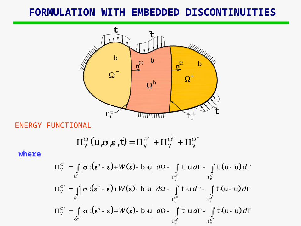
FORMULATION WITH EMBEDDED DISCONTINUITIES
V
V
V
: b u t u t u u
: b u t u t u u
: b u t u t u u
u
h
h h h
u
u
u
u
u
W d d d
W d d d
W d d d
ENERGY FUNCTIONAL
V V V Vu, , , th
where
n
i-
-
i
(2)(1)
h
n
+
+
tt
t
b b b
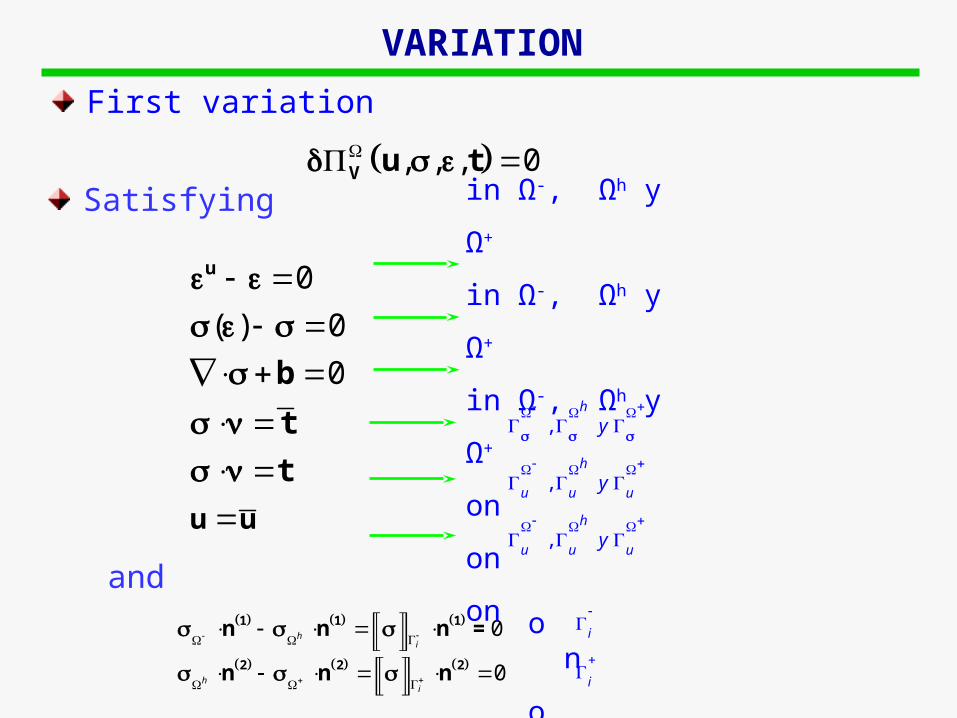
VARIATION
0
( ) 0
0
u
u u
b
t
t
0
0
hi
hi
1 1 1
2 2 2
n n n =
n n n
,
,
,
h
h
u u u
h
u u u
y
y
y
First variation
, , , 0 V u tSatisfying
in Ω-, Ωh y Ω+
in Ω-, Ωh y Ω+
in Ω-, Ωh y Ω+
on
on
on
and
i
i
on
on

APPROXIMATION BY EMBEDDED DISCONTINUITIES
Functional energy of the continuum
where
Continuum Approach a) Weak discontinuity
\V \ V V V V V, , , , ,
S SSS S
u u
\V
\
: b u t u u u tu
S u
S
W d d d
V : b uuh
S
k W d
a) b)
- n
h
n
k=0
+-
h
k=0
+
SS
-
+i-
i+
-
+
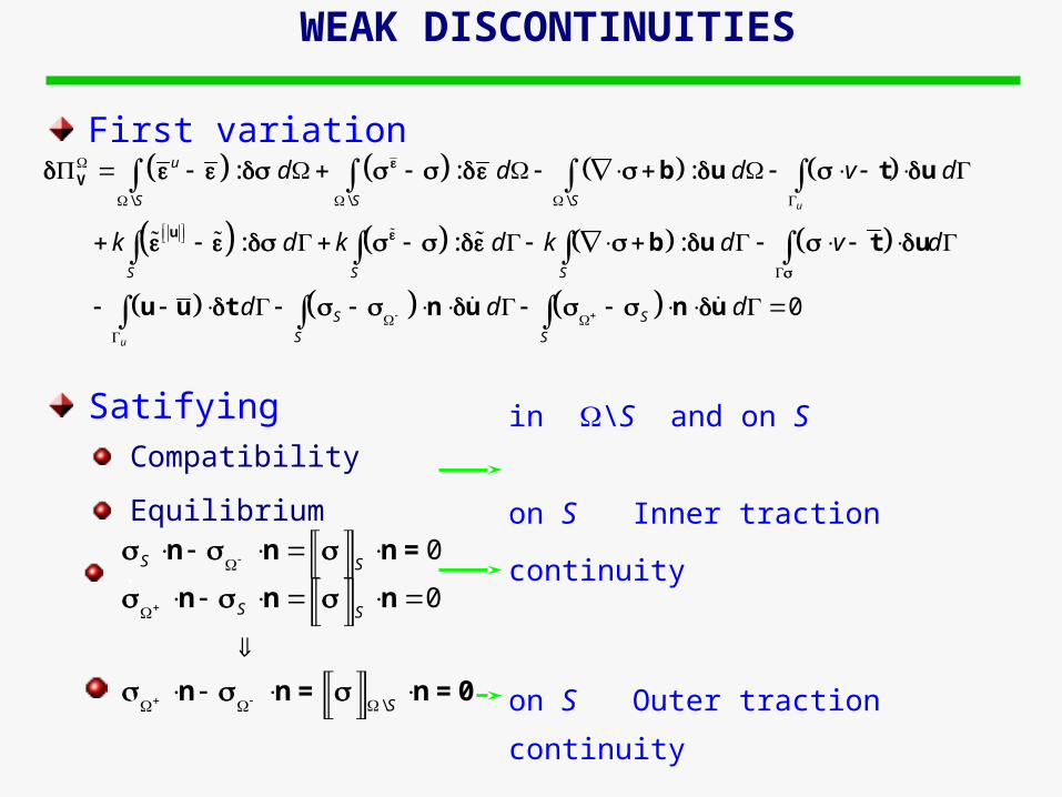
WEAK DISCONTINUITIES
\ \ \
: : :
: : :
0
V
u
b u t u
b u t u
u u t n u n u
u
u
u
S S S
S S S
S S
S S
d d d v d
k d k d k d v d
d d d
First variation
Satifying
\
0
0
S S
S S
S
n n n =
n n n
n n = n = 0
.
.
in \S and on S
on S Inner traction continuity
on S Outer traction continuity
Compatibility
Equilibrium

AC
V : uS
S
W d
Energy functional of the continuum
where
b) Strong discontinuity
\V
\
: b u t u u u tu
S u
S
W d d d
\V \ V V, , , , ,
SSS S
u u
+-
k=0
n -+
k=0
S
SS
i-
i+
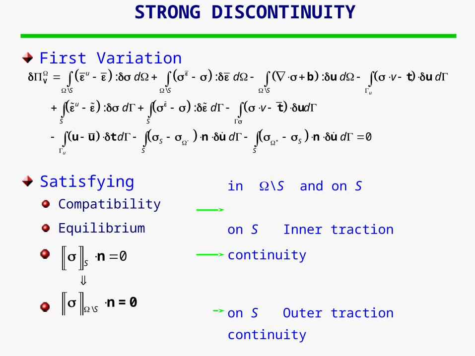
STRONG DISCONTINUITY
\ \ \
: : :
: :
0
u
u
u
S S S
u
S S
S S
S S
d d d v d
d d v d
d d d
V b u t u
t u
u u t n u n u
First Variation
SatisfyingCompatibility
Equilibrium
\
0S
S
n
n = 0
in \S and on S
on S Inner traction continuity
on S Outer traction continuity
.
.
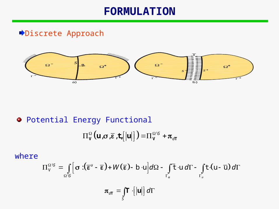
FORMULATION
Discrete Approach
Potential Energy Functional
where
\, , , Sd V V Tu t, u
d
S
d T T u
\V
\
: b u t u t u uu
S u
S
W d d d
-+
a) b)
+- Sn
+
S- S+
--+

AD
\ \ \
-
: : :
0
u u
u
S S S
S S S S
S S
d d d
v d v d d
T d T d
V b u
t u t u u u t
n u n u
First variation
Satisfying
\
0
0
S S
S S
S
T
T
n n =
n n
n n = n = 0
.
.
in \S y on S
on S Inner traction continuity
on S Outer traction continuity
Compatibility
Equilibrium

SUMMARY OF MIXED ENERGY FUNCTIONALS
Continuum Approach
VM \ \
\
, , , , , : ( )
: ( )
uS S S
S
S
S
W d d
W dS
u
u u b u t u
VM \ \
\
ˆ, , , : ( )uS S
S
S
W d d
T dS
T u u b u t u
u
Discrete Approach
VM \ \
\
, , , , , : ( )
: ( )
uS S S
S
S
S
W d d
k W dS
u
u u b u t u
b u
b) Strong discontinuity
a) Weak discontinuity
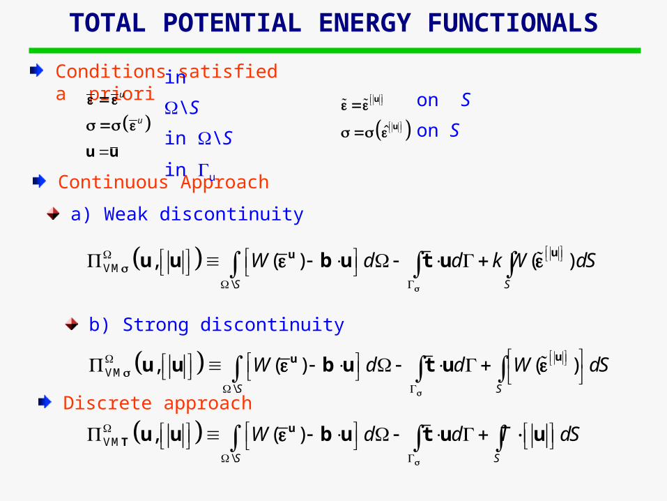
TOTAL POTENTIAL ENERGY FUNCTIONALS
VM
\
, ( ) ( )S S
W d d k W dS
uuu u b u t u
ˆ
u
u
Continuous Approach
VM
\
, ( ) ( )S S
W d d W dS
uuu u b u t u
VM
\
, ( )S S
W d d T dS
uT u u b u t u u
Discrete approach
b) Strong discontinuity
a) Weak discontinuity
Conditions satisfied a priori
u
u
u u
in \S
in \S
in u
on S
on S

TOTAL COMPLEMENTARY ENERGY FUNCTIONALS
\ \
\
, ( ) ( )u
S S S S
S S
W d d k W dS
VM n u
Continuous Approach
VM \ \
\
, ( ) ( )u
S S S S
S S
W d d W dS
n u
VM \ \
\
, ( )u
S S S S
S S
W d d dS
T n u n u
Discrete approach
b) Strong discontinuity
a) Weak discontinuity
Where\ \ \ \
1( ) : :
2S S S SW D
Conditions satisfied a priori
σ + b = 0
σ t
in \S
on σ

1. MIXED FEM
VM VM VM
1 2
0; 0; ... 0nu u u
VM VM 0 For to be stationary
Interpolation of fields
\
ˆ
· ·
\
( , ) ( ) ( )
ˆ( , ) ( ) ( )
( , ) ( ) ( )S S
c
S S
t
t
t
ee
u x N x d N x u
x N x e N x e
x N x N x
\
ˆ
·
\
( , ) ( ) ( )
ˆ( , ) ( )
( , ) ( )S
c
S
t
t
t
e
u x N x d N x u
x N x e
x N x
( )
1
k
u
u
d -B x u
u n
Dependent fields
CA DA

MIXED MATRICES
\
\
\
\ \\
ˆ ˆ ˆ
ˆ ·
\
·
ˆ
S
S S
S
S
S SS
SS
S
S
K
d
ext
u u
ee e
ee e
d eu
eu
d0 0 0 0 K 0F
0 0 0 0 K K u0
0 0 K 0 K 0 e 00 0 0 K 0 K 0e
K K 0 0 0 0
00 K 0 K 0 0
Discrete Approach
Continuum Approach
\
\
\
\ \\
ˆ ˆ ˆ
ˆ ·
\
ˆ
S
S
S
S SS
S
S
K
d ext
u
ee e
d eu
d0 0 0 K F0 0 0 K u
F0 0 K K
0eK K 0 0
u on S

DISPLACEMENT FEM
S
F
Interpolation of fields
Stiffness matrix
Continuum Approach
Discrete Approach
( ) ( ) Cu d +N x N x u
\ \
\ \
S S
S
S S
d d
d d
T TC
ext
T TC C C
B C B B C BFd
uB C B B C B F
S
S
S
S
d
d
n
T
1S
S
nk
u
T u

FORCE FEM
SFF
Interpolation of fields
Flexibility matrix
Continuum Approach
Discrete Approach
\\
· ·
( , ) ( ) ( )S SS St
x N x N x
\ \ \ \ \ \
\ \ \
·
\\ \
·
\ \
S S S S S S S
u
S S S S S S
SS S
S SS S
d d d
d d
T T T
T
N D N N D N n N u
N D N N D NFF
S
S
S
d
d
n u
:
:
CS S
S
DS S
S
d
d
D
n D

TENSION BAR PROBLEM
2
1000
1
0.005 /
2.0
1.0
u
E MPa
f MPa
G MN m
L m
A m
Properties
Geometryu
y
x
1
L
E, A2
2f
d2d1

MATRICES FOR THE LINEAR ELEMENT
1 1
2 2
11 1
1 1
L f dHf dEA
StiffnessFlexibility
1 1
2 2
1 1
1 1 1
d fEA
d fLH
1 1
2 2
1
2
1
2
0 0 0 0 02 2
0 0 0 0 02 2
0 0 0 0 02 2
00 0 03 6
00 0 0 06 3
00 0
2 2 2 3 6
0 02 2 2 6 3
A A
A A
d fA A d f
u EAHEA EA AL AL
eL L
eEA EA AL AL
L LA A A AL AL
A A A AL AL
Mixed

RESULTS
Load-displacement diagram Stress-jump diagram
0.002 0.004 0.006 0.008 0.010
0.2
0.4
0.6
0.8
1.0
00
[ u ] (m)
(
MP
a)
[ u ] =HEmáx
B
C
D
S
u
Gf
0.002 0.004 0.006 0.008 0.010
0.2
0.4
0.6
0.8
1.0
00
d (m)
P (
MN
)
B
A
C
D
Gf

2D IDEALIZATION
P
x
y
L
h
P
x
y
L
h
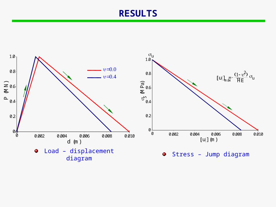
RESULTS
Load – displacement diagram Stress – Jump diagram
0.002 0.004 0.006 0.008 0.010
0.2
0.4
0.6
0.8
1.0
00
d (m)
P (
MN
)
0.002 0.004 0.006 0.008 0.010
0.2
0.4
0.6
0.8
1.0
00
[ u ] (m)
(M
Pa)
[ u ] = HEmáx
S
u
2
u

EVOLUTION TO FAILURE

CONCLUSIONS
A general variational formulation of the strain localization phenomenon and its discrete approximation were developed.
With the energy functionals developed in this work, it is possible to formulate Displacement, Flexibility and Mixed FE matrices with embedded discontinuities.
The advantage of this formulation is that the FE matrices are symmetric, with the stability and convergence of the numerical solutions, guaranteed at a reduced computational cost.
There is a relationship between the CA and DA in the Strong Discontinuity formulation not only in the Damage models, but also in their variational formulations.
FUTURE RESEARCH
Implement 2 and 3D formulations in a FE with embedded discontinuities code to simulate the evolution of more complex structures to collapse.


