Page 1
Variationally Consistent Methods for Lagrangian Dynamicsin Continuum Mechanics
by
Sudeep K. Lahiri
Submitted to the Department of Aeronautics and Astronauticsin partial fulfillment of the requirements for the degree of
Doctor of Philosophy
at the
MASSACHUSETTS INSTITUTE OF TECHNOLOGY
r~y2006L, e., ;( 0 0
@ Massachusetts Institute of Technology 2006. All rights reserved.
Author)M- c0 autics and stronautics
A 14aA 26, 2006
Certified by-
Certified by
Certified by
Certified b.
Accepted by
MASSACHUSETTS INSOF TECHNOLOC
JUL 11 200
LIBRARIIE
A
N.Jaim Peraire
P rofes A autic. ad Astronautics
( psis Supervisor
-
\ssn / 9 Astronautics
-l ov izkystan fa e ics Aed Alrpnautics
Jann -''eraireProfessor of Aeron s and Astronautics
y T Chair, Committee on Graduate Students
7
S
12
iRCHtVES
Page 3
Variationally Consistent Methods for Lagrangian Dynamics in
Continuum Mechanics
by
Sudeep K. Lahiri
Submitted to the Department of Aeronautics and Astronauticson May 26, 2006, in partial fulfillment of the
requirements for the degree ofDoctor of Philosophy
Abstract
Rapid dynamics are commonly encountered in industrial applications such as forging, crashtests and many others. These problems are typically non-linear due to large deformationsand/or non-linear constitutive relations. Such problems are typically modelled from a La-grangian viewpoint, where the mesh is attached to the body; hence, large deformations leadto large distortions in the mesh. Explicit numerical methods are considered to be efficient inthese cases where large meshes and small time-steps are employed for spatial and temporalresolution. However, incompressible and nearly incompressible materials pose a problem asthe timestep stability restriction in explicit methods becomes increasingly severe.
Most of the numerical methods employed for such simulations, are developed from dis-cretization of the equations of motion. Recently, Variational Integrators have been devel-oped where the numerical time integration scheme is developed from a variational principlebased on Hamilton's principle of stationary action. Such methods ensure conservation oflinear and angular momentum, which lead to more physically consistent simulations.
In this research, numerical methods addressing incompressibility and mesh distortionshave been developed under a variational framework. A variational formulation for meshadaptation procedures, involving local mesh changes for triangular meshes, is presented.Such procedures are very well suited for explicit methods, without significant expense.Conservation properties of such methods are proved and demonstrated. Further, a Frac-tional Time-Step method is developed, from a variational framework, for incompressible andnearly incompressible problems. Algorithmic details are presented, followed by examplesdemonstrating the performance of the method.
Thesis Supervisor: Jaime PeraireTitle: Professor of Aeronautics and Astronautics
3
Page 5
ya nisha sarva-bhutanam, tasyam jagarti sanyami I
yasyam jagrati bhutani, sa nisha pashyato muneh ||
... Shrimad Bhagavad Gita
Chapter 2.
"What is night for all beings, is the time of awakening for the self-controlled;
and the time of awakening for all beings, is night for the introspective sage."
I dedicate this thesis to my mother Mrs. Namita Lahiri
and my father Mr. Salil Kumar Lahiri.
5
Page 7
Acknowledgments
It has been a privilege to be a part of MIT. I am indeed indebted to be in the PhD program
at the department of Aeronautics and Astronautics.
I am grateful to my advisor, Prof. Jaime Peraire who has guided me all along the course
of the program with great patience and enthusiasm. I am also grateful to Prof. Javier
Bonet, (University of Wales, Swansea, UK.) who as been like a co-advisor to me all through
my research. Both of them have given me directions and advice without which this thesis
would not have completed. I am indebted to them for introducing me to the world of
variational integrators and mesh adaptation.
I would like to thank Dr Jim Stewart, from Sandia National Laboratory, for the research
discussions and support to the project. I am indebted to the financial support from Sandia
National Laboratory, USA.
I would also like to thank various faculty members of the department, especially Prof.
Raul Radovitzky, with whom I had many insightful discussions regarding my research and
continuum mechanics in general. I would also like to thank various faculty members like
Prof. Mark Drela (Aero-Astro., MIT), Prof. K. J. Bathe (Mech. E., MIT), Prof. Simona
Socrates (Mech. E., MIT) and Prof. John Hutchinson (Harvard University) whose teaching
and course-work, helped me build my background in the area of continuum mechanics. I
would especially like to thank Prof. Steven Hall, and the department of Aeronautics and
Astronautics, for providing a great opportunity by offering a Graduate Teaching Fellowship
for the course of Unified Engineering in the department. It was really a privilege to be the
part of the Unified Staff and the teaching workshops conducted by Prof. Paul Lagace was
highly thought provoking.
I am also grateful to be a part of ACDL (Aerospace Computational Design Laboratory)
for creating such a nice and conducive academic and research environment, which helped
me endure the challenges of the PhD program with sanity. I would like to thank Mr. Bob
Haimes, who has been a great source of learning for me, from whom I learned a lot of
programming and associated issues. I would like to thank Jean Sofranos, for her help in
schedules and various lab activities. I would particularly like to thank all my co-students
7
Page 8
at ACDL, interacting with whom was a great source of learning and fun. I would like to
remember the company of my co-students like David Venditti, Victor Garzon, Tolulope
Okusanya, Giuseppe Alescio, James Lu, Sean Bradshaw and especially David Willis as
great moments of sharing, interactive learning and hectic activity. Discussions ranged from
computations to mathematics, physics, politics, sports(cricket), society etc., which was
indeed very educative, as well as very befriending. It was also enriching to interact with
some of the new members, Garrett Barter, Krzysztof Fidkowski, Todd Oliver, Theresa
Robinson and Tan Bui, who are very enthusiastic and are really very helpful and friendly.
I would especially like to thank Garrett, Krzystoff and Todd, for their active support not
only to me but to the whole lab in affairs of software support.
It has been a great experience in the department of Aeronautics and Astronautics, with
great staff members, like Marie Stuppard and Barbara Lechner, who have been extremely
nice and considerate to students' issues, without whose support, graduate study would have
been very inconvenient.
Finally and most importantly I would like to thank my mother Mrs. Namita Lahiri, and
my father Mr. Salil Kumar Lahiri, for their blessings and active support all through my
academic career and life so far, without whose sacrifices and initiatives, it would have been
extremely hard to avail such a great opportunity of learning and experience. I would also
like to thank my sisters and my entire family who have been really concerned and helpful
in my activities.
8
Page 9
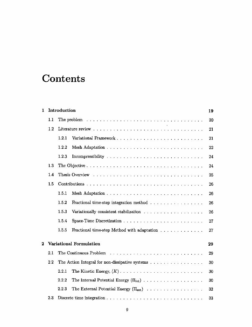
Contents
1 Introduction
1.1 The problem . . . . . . . . . .
1.2 Literature review . . . . . . . .
1.2.1 Variational Framework .
1.2.2 Mesh Adaptation . . . .
1.2.3 Incompressibility . . . .
1.3 The Objective . . . . . . . . . .
1.4 Thesis Overview . . . . . . . .
1.5 Contributions . . . . . . . . . .
1.5.1
1.5.2
1.5.3
1.5.4
Mesh Adaptation . . . . . . .
Fractional time-step integratio
Variationally consistent stabili
Space-Time Discretization . .
19
. . . . . . . . . . . . . . . . . . . . . . 2 0
. . . . . . . . . . . . . . . . . . . . . . 2 1
. . . . . . . . . . . . . . . . . . . . . . 2 1
. . . . . . . . . . . . . . . . . . . . . . 2 2
. . . . . . . . . . . . . . . . . . . . . . 2 4
. . . . . . . . . . . . . . . . . . . . . . 2 4
. . . . . . . . . . . . . . . . . . . . . . 2 5
. . . . . . . . . . . . . . . . . . . . . . 2 6
. . . . . . . . . . . . . . . . . . . . . . 2 6
n method . . . . . . . . . . . . . . . . 26
zation . . . . . . . . . . . . . . . . . . 26
. . . . . . . . . . . . . . . . . . . . . . 2 7
1.5.5 Fractional time-step Method with adaptation
2 Variational Formulation
2.1 The Continuous Problem . . . . . . . . . . . . . . .
2.2 The Action Integral for non-dissipative systems . . .
2.2.1 The Kinetic Energy, (K) . . . . . . . . . . . .
2.2.2 The Internal Potential Energy (Hint) . . . . .
2.2.3 The External Potential Energy (Hext) .
2.3 Discrete time integration . . . . . . . . . . . . . . . .
9
27
29
29
30
30
30
32
33
Page 10
2.4 Conservation of System Invariants . . . . . .
2.4.1 A simple example: System of Particles
2.5 Space-Time Discretization . . . . . . . . . . .
2.6 Standard finite element formulation . . . . .
2.7 Averaged nodal element formulation . . . . .
2.8 Stabilized element . . . . . . . . . . . . . . .
2.8.1 Stiffness stabilization . . . . . . . . . .
2.8.2 Viscous stabilization . . . . . . . . . .
3 Mesh Adaptation
3.1 Diagonal Swapping . . . . .
3.2 Edge Splitting . . . . . . . .
3.3 Node Movement . . . . . .
3.4 Edge Collapsing . . . . . . .
3.5 Implementation . . . . . . .
3.5.1 Error Estimate . . .
3.5.2 Adaptation Criteria
3.6 Mesh Adaptation Examples
3.6.1 Spinning Plate . . .
3.6.2 An oscillating ring
3.6.3 A Tensile test case
3.6.4 A Punch test . . . .
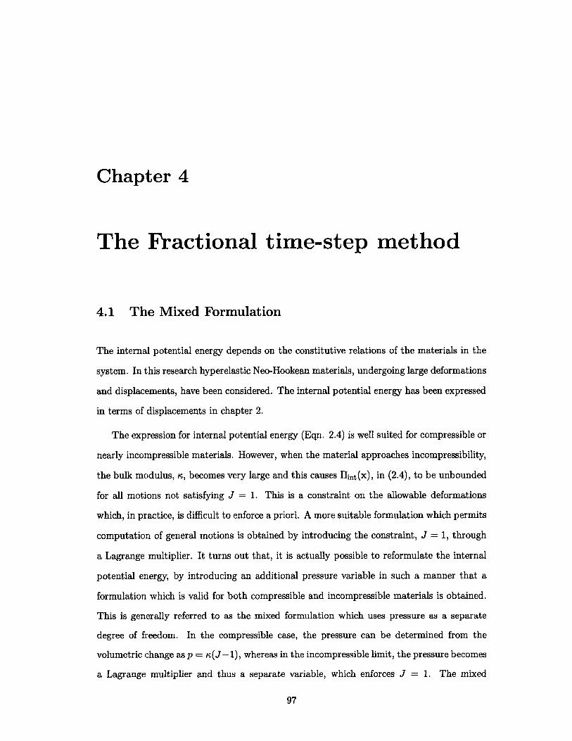
3.6.5 Plate Impact . . . .
3.7 Concluding Remarks . . . .
4 The
4.1
4.2
4.3
Fractional time-step method
The Mixed Formulation . . . . . . . . .
Fractional Step Variational Formulation
Finite Element Spatial Discretization . .
4.4 Linearized Formulation . . . . . . . . . . . . . . . . . . . . . . . . . . . . . .
4.4.1 Linearization of the volume increment . . . . . . . . . . . . . . . . .
10
35
37
38
44
48
52
52
54
65
. . . . . . . . . . . . . . . . . . . . . . . . . . 6 5
. . . . . . . . . . . . . . . . . . . . . . . . . . 6 8
. . . . . . . . . . . . . . . . . . . . . . . . . . 7 0
. . . . . . . . . . . . . . . . . . . . . . . . . . 7 3
. . . . . . . . . . . . . . . . . . . . . . . . . . 7 9
. . . . . . . . . . . . . . . . . . . . . . . . . . 7 9
. . . . . . . . . . . . . . . . . . . . . . . . . . 8 3
. . . . . . . . . . . . . . . . . . . . . . . . . . 8 5
. . . . . . . . . . . . . . . . . . . . . . . . . . 8 5
. . . . . . . . . . . . . . . . . . . . . . . . . . 8 7
. . . . . . . . . . . . . . . . .. . . . . . . . . 8 8
. . . . . . . . . . . . . . . . . . . . . . . . . . 90
. . . . . . . . . . . . . . . . . . . . . . . . . . 9 0
. . . . . . . . . . . . . . . . . . . . . . . . . . 9 5
97
97
98
100
102
102
Page 11
4.4.2 First step . . . . . .
4.5 Linear Stability Analysis .
4.6 Pressure Stabilization . .
4.7 Examples . . . . . . . . . .
4.7.1 A Plane Strain Case
4.7.2 A spinning plate
4.7.3 2D Beam bending
4.8 Concluding Remarks . . . .
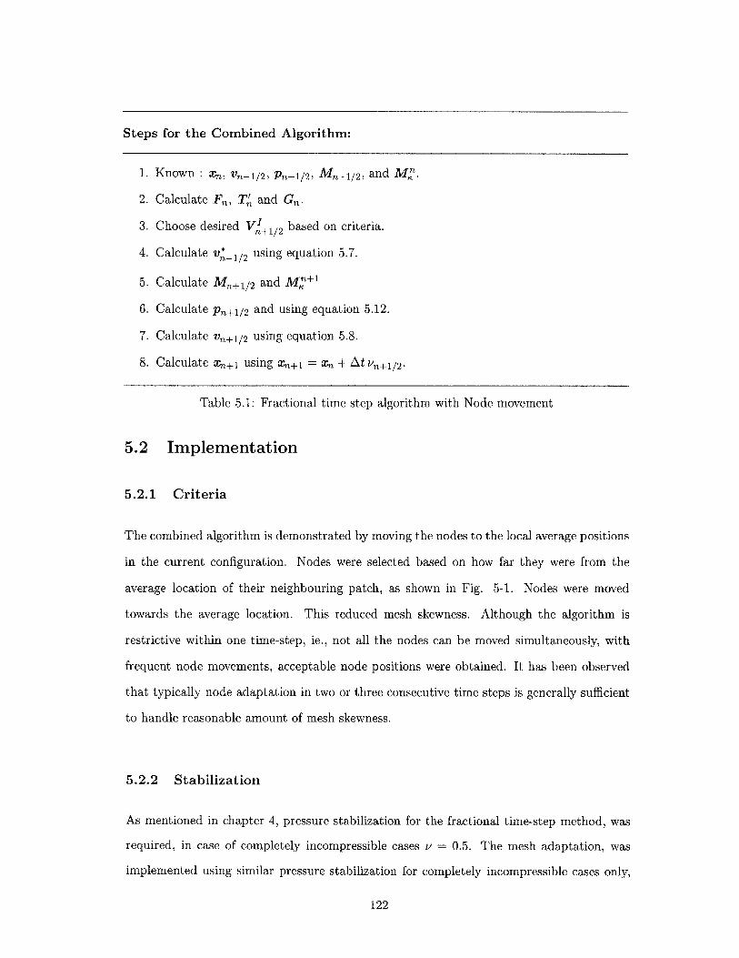
5 Fractional time-step method
5.1 Variational Formulation . .
5.2 Implementation . . . . . . .
5.2.1 Criteria . . . . . . .
5.2.2 Stabilization . . . .
5.3 Examples . . . . . . . . . .
5.3.1 A Spinning plate . .
5.3.2 Beam Bending . . .
5.4 Concluding remarks . . . .
6 Conclusions
6.1 Summary . . . . . . . . . . . . . . . . . . . . . . . . . . . . . . . . . . . .
6.2 Future work . . . . . . . . . . . . . . . . . . . . . . . . . . . . . . . . . . .
with mesh adaptation
103
104
107
108
108
111
111
115
117
118
122
122
122
123
123
123
129
131
131
133
11
Page 13
List of Figures
2-1 Continuous systems . . . . . . . . . . . . . . . . . . . . . . . . . . . . . . .
2-2 A system of particles . . . . . . . . . . . . . . . . . . . . . . . . . . . . . . .
2-3 The space-time-prism (left) and a generic space-time-tetrahedron (right). .
2-4 A schematic of the beam bending case used to demonstrate the performance
of the standard and averaged nodal element. . . . . . . . . . . . . . . . . .
2-5 The standard element (left) shows excessive stiff behaviour undergoing less
deformation. The averaged nodal element (right) does not show any volu-
metric locking, undergoing larger deformations. . . . . . . . .
2-6 The averaged nodal element shows shear locking (left) which is
the stabilized element (right) . . . . . . . . . . . . . . . . . . .
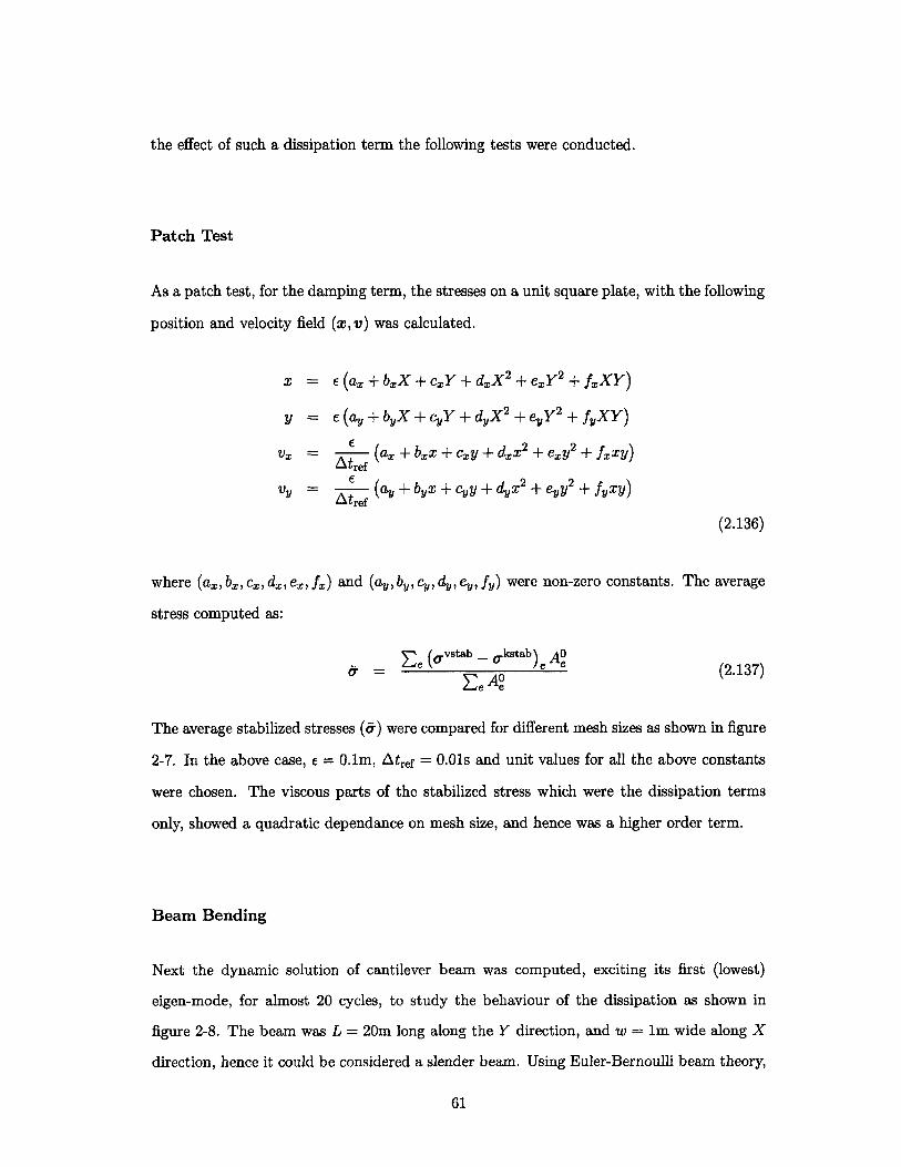
2-7 Patch test showing the mesh dependancy of the viscous parts of
stabilized stresses. . . . . . . . . . . . . . . . . . . . . . . . . .
2-8 The energy history and the tip deflection for cantilever beam.
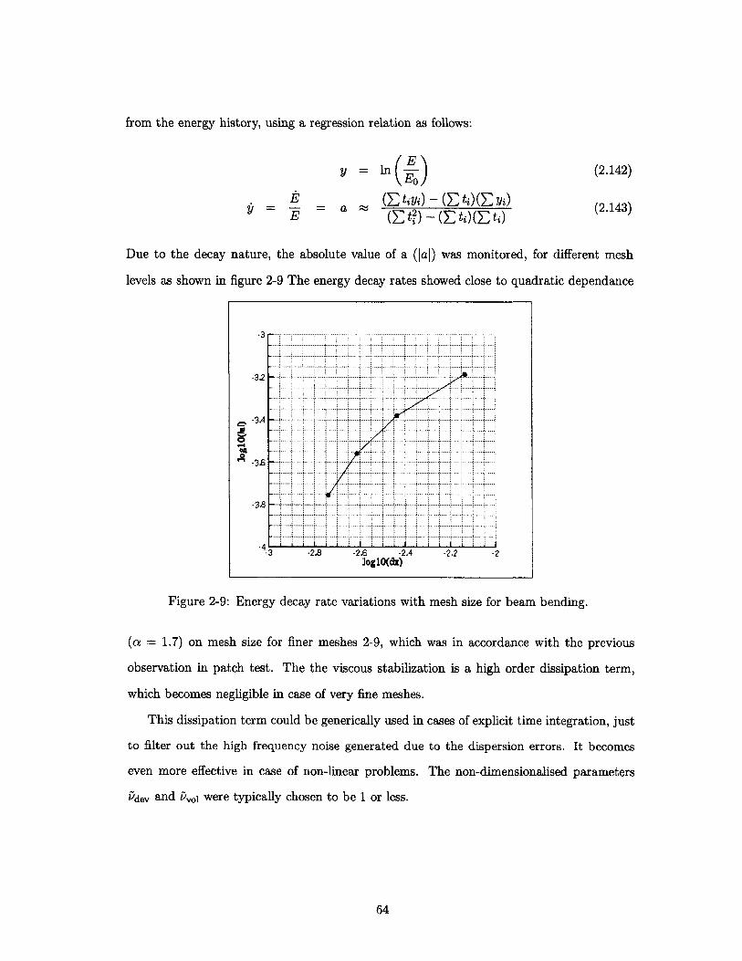
2-9 Energy decay rate variations with mesh size for beam bending.
3-1
3-2
3-3
3-4
3-5
3-6
3-7
3-8
. . . . . . . 53
rectified by
54
the average
. . . . . . . 62
. . . . . . . 63
. . . . . . . 64
The space-time volume for the diagonal swapping. . . . . . . . . . . . . . .
The space-time volume for edge splitting. . . . . . . . . . . . . . . . . . . .
Understanding node movement with an intermediate mapping. . . . . . . .
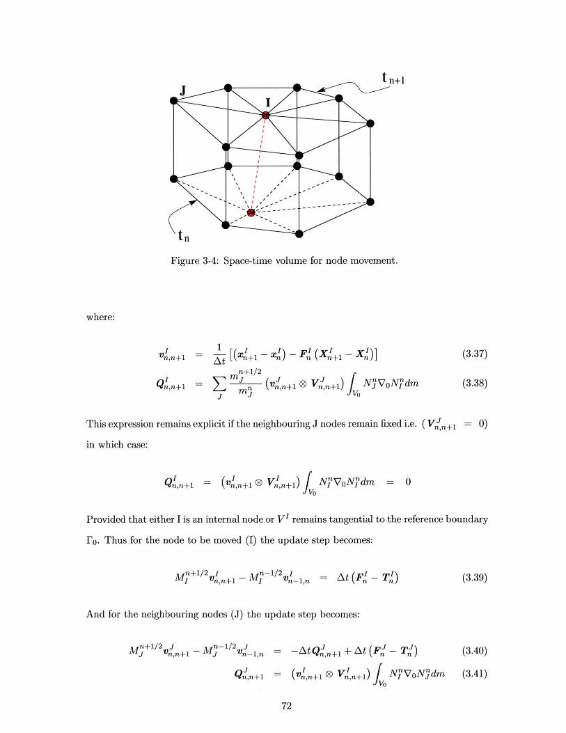
Space-time volume for node movement. . . . . . . . . . . . . . . . . . . . .
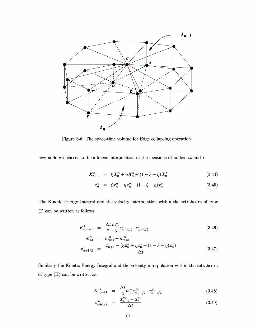
Collapsing the edge ab to the point c. . . . . . . . . . . . . . . . . . . . . .
The space-time volume for Edge collapsing operation. . . . . . . . . . . . .
The subdivision of the space-time volume into different types of tetrahedra.
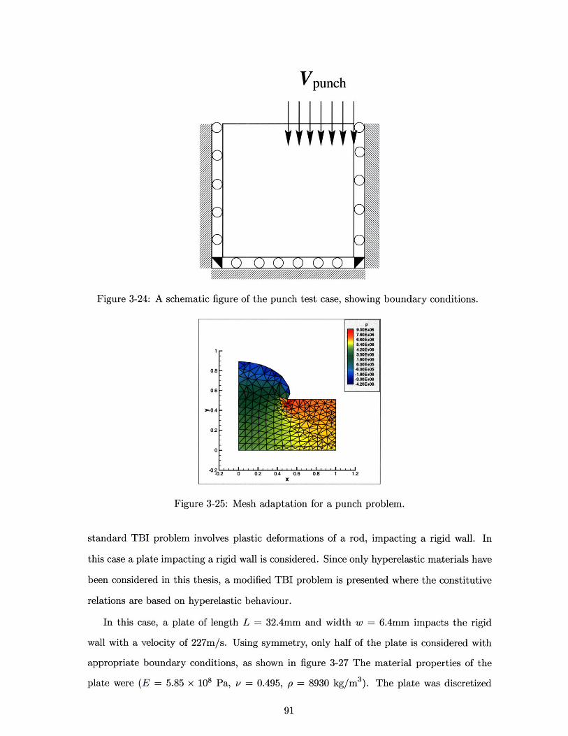
A schematic of the punch test case. . . . . . . . . . . . . . . . . . . . . . .
66
68
71
72
73
74
75
81
13
29
37
39
53
Page 14
3-9
3-10
3-11
3-12
3-13
3-14
3-15
3-16
3-17
3-18
3-19
3-20 Deformation at intermediate step with adaptation.
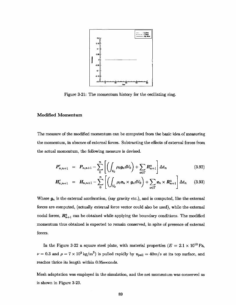
The momentum history for the oscillating ring. . . . . . . . . . . . . . .
A Tensile test specimen (left) pulled to thrice its length (right). . . . . .
The Modified Momentum history for the Tensile test . . . . . . . . . . . .
A schematic figure of the punch test case, showing boundary conditions.
Mesh adaptation for a punch problem. . . . . . . . . . . . . . . . . . . . .
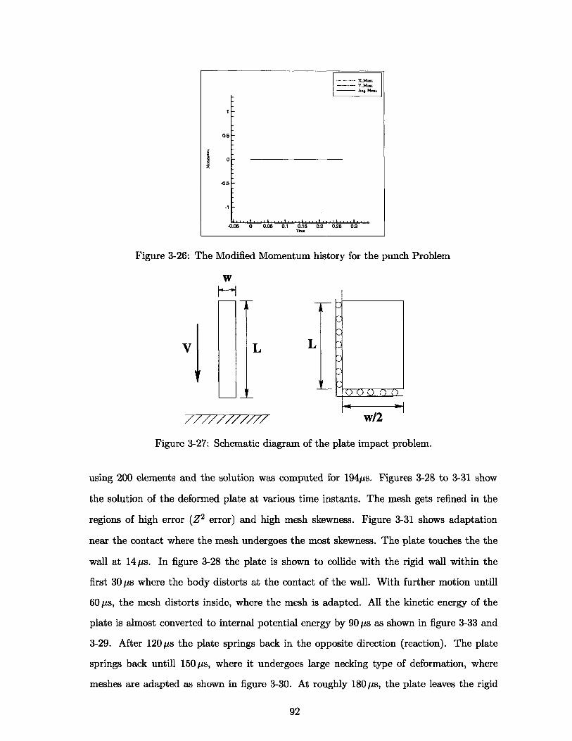
The Modified Momentum history for the punch Problem . . . . . . . . . .
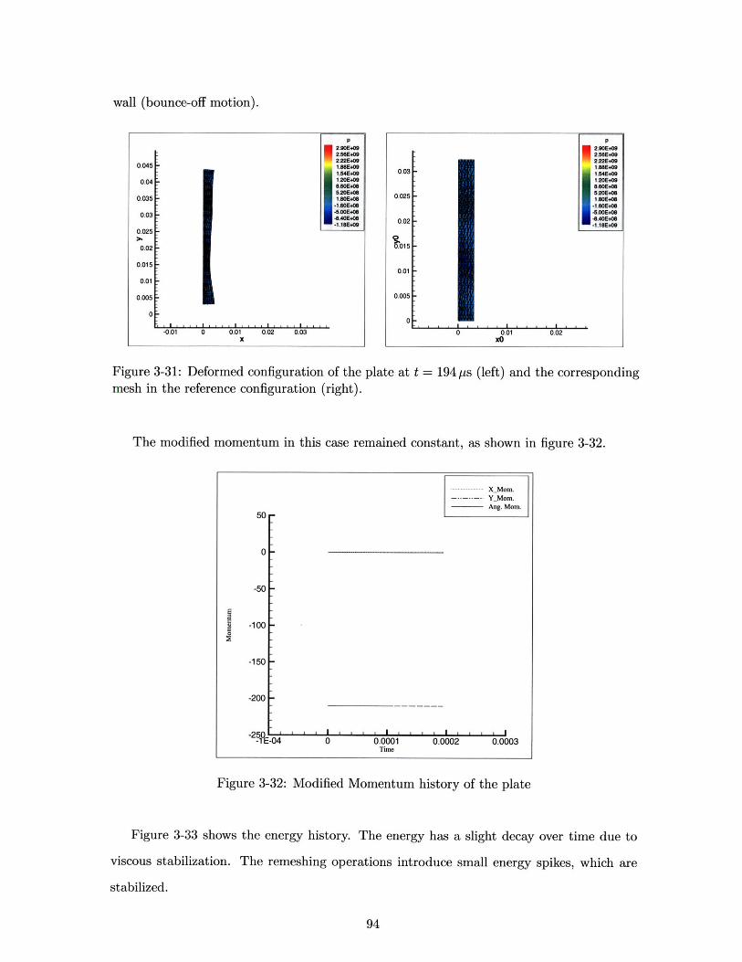
3-27 Schematic diagram of the plate impact problem.
3-28 The plate at t = 30 ps (left) and t = 60 ps (right).
3-29 The plate at t = 90 ps (left) and t = 120 ps (right).
3-30 The plate at t = 150 ps (left) and t = 180 ps (right).
3-31 Deformed configuration of the plate at t = 194 ps (left)
mesh in the reference configuration (right). . . . . .
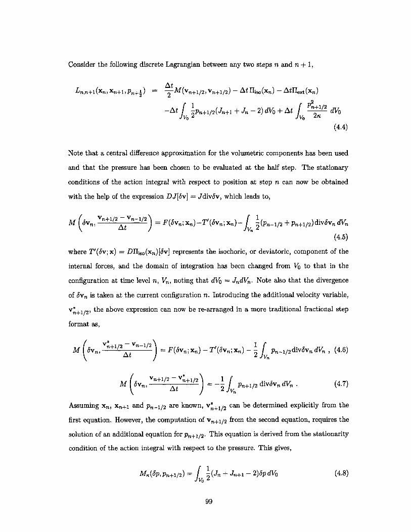
3-32 Modified Momentum history of the plate . . . . . . .
3-33 The Energy history. . . . . . . . . . . . . . . . . . .
and the corresponding
Two dimensional test case . . . . . . . . . . . . . . . . . . . . . . . . . . . .
Displacement of point X1 = 1, X 2 = 0 in time for nearly incompressible
solution (v = 0.4999) compared with analytical solution. . . . . . . . . . . .
14
Error in stresses xx.. . . . . . . . . . . . . . . . . . . . . . . . . . . . . . . .
Error in stress .. . . . . . . . . . . . . . . . . . . . . . . . . . . . . . . .
Error in stress agy. . . . . . . . . . . .
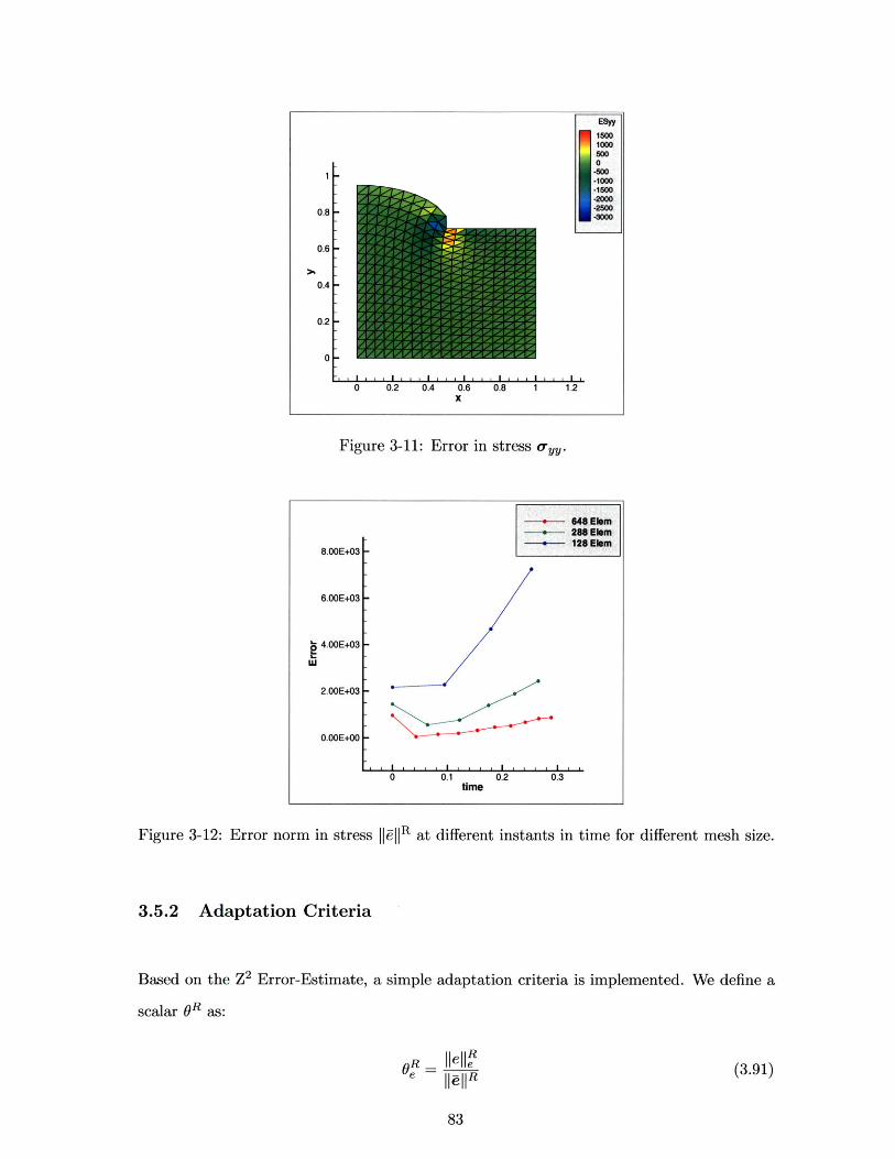
Error norm in stress ||E||R at different instants in time for different mesh size.
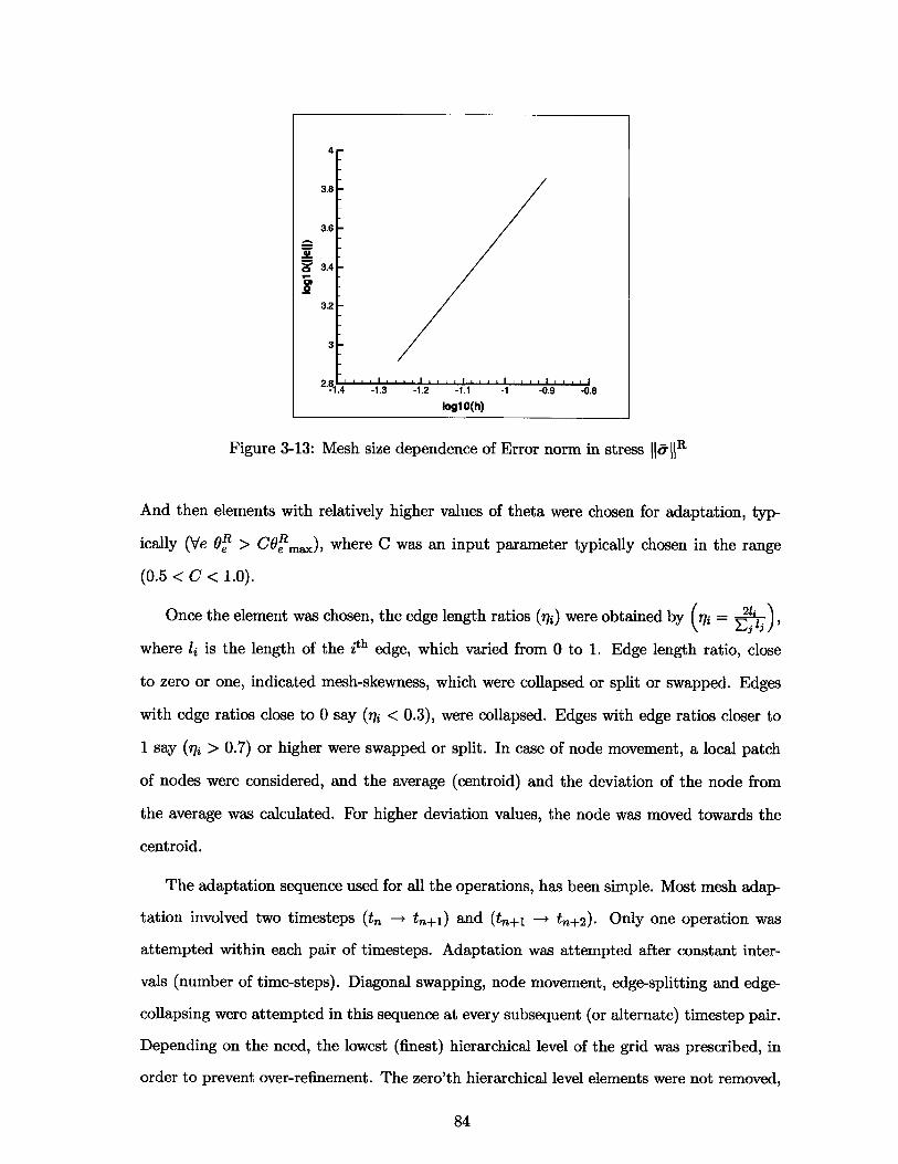
Mesh size dependence of Error norm in stress |||R .............
A Spinning plate simulation with adaptation. . . . . . . . . . . . . . . . .
Linear and angular momentum history . . . . . . . . . . . . . . . . . . . . .
Location of center of mass. . . . . . . . . . . . . . . . . . . . . . . . . . . .
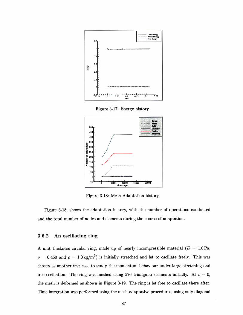
Energy history. . . . . . . . . . . . . . . . . . . . . . . . . . . . . . . . . .
Mesh Adaptation history. . . . . . . . . . . . . . . . . . . . . . . . . . . . .
A circular ring(left) is initially stretched(right) and let to oscillate freely. . .
3-21
3-22
3-23
3-24
3-25
3-26
82
82
83
83
84
85
86
86
87
87
88
. . . . . . . . . . . . 8 8
89
90
90
91
91
92
92
93
93
93
94
94
95
108
110
4-1
4-2
Page 15
4-3 Displacement of point X1 = 1, X 2 = 0 in time for incompressible solution
(v = 0.5) compared with analytical solution. . . . . . . . . . . . . . . . . . .
Energy History. . . . . . . . . . . . . . . . . . . . . . . . . . . . .
Spinning plate test case. . . . . . . . . . . . . . . . . . . . . . . .
Finite element mesh and pressure distribution at a given instant.
Linear momentum and angular momentum plots. . . . . . . . . .
Beam bending . . . . . . . . . . . . . . . . . . . . . . . . . . . . .
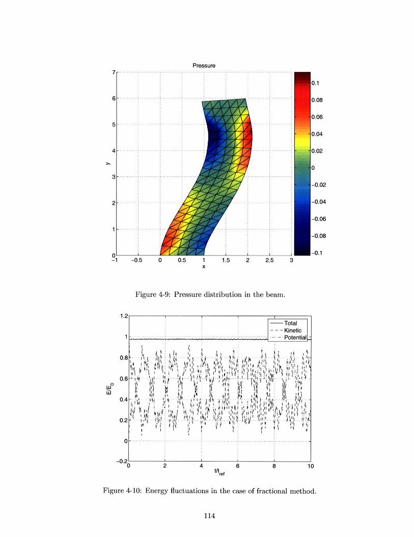
Pressure distribution in the beam. . . . . . . . . . . . . . . . . .
Energy fluctuations in the case of fractional method. . . . . . . .
Dependency of maximum stable timestep on bulk modulus . . . .
. . . . . . 111
. . . . . . 112
. . . . . . 112
. . . . . . 113
................... .. .... 113
. . . . . . 114
. . . . . . 114
. . . . . . 115
4-4
4-5
4-6
4-7
4-8
4-9
4-10
4-11
5-1
5-2
5-3
5-4
5-5
5-6
5-7
5-8
5-9
5-10
5-11
5-12
5-13
117
118
124
124
125
125
126
126
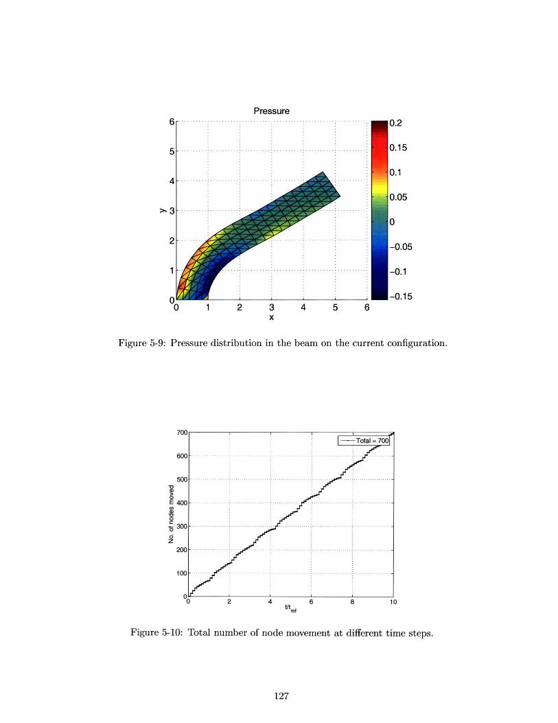
127
127
128
128
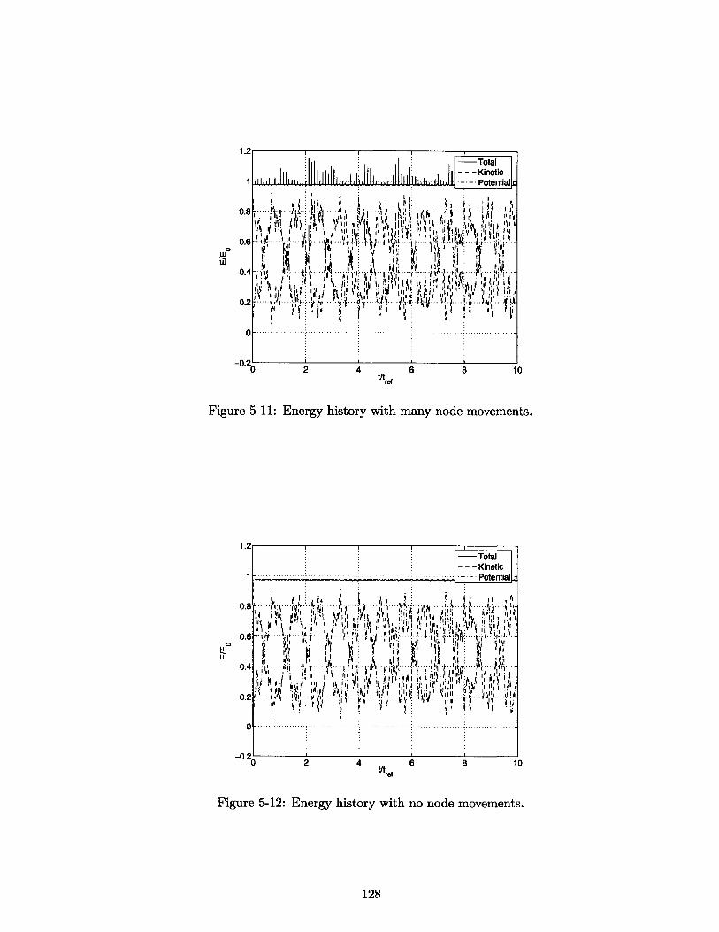
129
15
110
Space-time volume for node movement. . . . . . . . . . . . . . . . . . . . .
Node movement with an intermediate mapping. . . . . . . . . . . . . . . .
Pressure distribution on the spinning plate at the current configuration. . .
The pressure distribution in the reference configuration of the spinning plate.
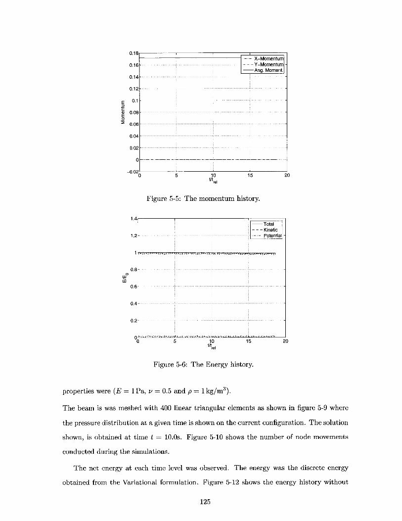
The momentum history. . . . . . . . . . . . . . . . . . . . . . . . . . . . .
The Energy history. . . . . . . . . . . . . . . . . . . . . . . . . . . . . . . .
The Adaptation history showing the total number of node movements con-
ducted. . . . . . . . . . . . . . . . . . . . . . . . . . . . . . . . . . . . . . .
Beam bending . . . . . . . . . . . . . . . . . . . . . . . . . . . . . . . . . . .
Pressure distribution in the beam on the current configuration. . . . . . . .
Total number of node movement at different time steps. . . . . . . . . . . .
Energy history with many node movements. . . . . . . . . . . . . . . . . . .
Energy history with no node movements. . . . . . . . . . . . . . . . . . . .
Incorrect pressure distribution(left) corrected by the use of pressure stabi-
lization (right). . . . . . . . . . . . . . . . . . . . . . . . . . . . . . . . . . .
Page 17
List of Tables
4.1 Fractional time step algorithm . . . . . . . . . . . . . . . . . . . . . . . . . 104
5.1 Fractional time step algorithm with Node movement . . . . . . . . . . . . . 122
17
Page 19
Chapter 1
Introduction
Rapid dynamics encompasses a significant section of continuum mechanics problems. Sev-
eral industrial phenomena involve rapid dynamics of solids, for example forging, machining,
crash-tests, collision modelling and many others. Computational simulations of such prob-
lems are used in various engineering analysis and design. These problems involve large
deformations and rotations along with complex material behaviour. Hence these problems
are inherently non-linear. Due to high velocities (of the order of speed of sound in the ma-
terial), large meshes and many small time-steps are used for spatial and temporal accuracy.
Hence explicit time-integrators become advantageous in such applications. Several codes
have been developed and used for such problems [1, 2, 3, 4], based on explicit methods.
The main challenges in these numerical problems lie in the proper modelling of large defor-
mations and rotations, modelling of contact, and modelling of complex non-linear material
behaviour. Explicit methods have a maximum allowable time-step limitation from stabil-
ity considerations, which inversely depends on the fastest wave speed in the material. In
case of nearly incompressible materials, the fastest wave speed becomes very large, causing
the maximum allowable time-step to be very small. In case of completely incompressible
materials explicit methods cannot be used. Thus incompressibility poses problems in use
of explicit methods. One way to address this problem due to incompressibility is by using
mixed formulations, where pressure is an additional degree of freedom. Mesh distortions,
encountered due to large deformations/rotations lead to lack of accuracy of the solution.
Problems due to mesh distortions have been addressed by mesh adaptation.
19
Page 20
An important aspect of a time-integration method in dynamics applications is its abil-
ity to conserve mass, momentum (linear and angular) and energy, which leads to more
physically consistent solutions. Methods which do not have good conservation properties,
develop large errors under long time-integrations. Typically dynamics in solids are mod-
elled from a Lagrangian formulation of the equations of motion. Hence mass conservation
is automatically satisfied in such methods. Exact conservation of global energy is hard
to obtain. But global momentum (linear and angular) conservation is possible. The ex-
plicit time-integrator, the Central Difference Scheme (also called the Leap-Frog Method in
fluid mechanics), is found to conserve global momentum exactly. Existing codes [3, 4] have
employed this method with great success.
Recent research [5] has shown that time-integration methods developed from a varia-
tional principle as that of Hamilton's principle of stationary action, necessarily conserve
linear and angular momentum. Such methods are commonly called as Variational Inte-
grators or Variational methods. The existing methods for mesh adaptation and mixed
formulation (to address incompressibility) used so far in present codes, are not derived from
a variational principle. Hence momentum conservation is not ensured in such methods. In
this thesis, the development of mesh adaptation and mixed formulation from a Variational
principle is presented.
1.1 The problem
Mesh distortion is an important problem in simulation of dynamics involving large deforma-
tions and rotations. Mesh adaptive updates can be used to reduce mesh distortions. Such
use of adaptation has been limited, since these updates add errors to the solution. Exist-
ing mesh-adaptive updates do not ensure conservation of momentum which lead to errors
over many time-integration steps. Hence, it is desired that such mesh updates conserve
global momentum which would allow use of adaptation in reducing mesh distortions and
also increase the accuracy of the solution.
Mixed formulations, where pressure is an additional unknown, are used to handle incom-
pressibility. Several methods exist to handle incompressible material behaviour [6]. Most of
20
Page 21
these methods are derived from discretizing the equations of motion, therefore, these meth-
ods do not ensure conservation of momentum. Hence, a variationally consistent method
employing a mixed formulation that ensures conservation of momentum is desired.
1.2 Literature review
1.2.1 Variational Framework
Variational integrators have been developed by several researchers [5, 7, 8, 9, 10, 11, 12, 13],
on the basis of Hamilton's principle of stationary action, rather than discretizing in time the
differential equations of motion. Hamilton's principle dictates that the path followed by a
body represents a stationary point of the action integral of the Lagrangian over a given time
interval [14, 15]. Variational integrators take advantage of this principle by constructing a
discrete approximation of this integral which then becomes a function of a finite number of
positions of the body at each timestep. The stationary condition of the resulting discrete
functional with respect to each body configuration leads to time stepping algorithms that
retain many of the conservation properties of the continuum problem. In particular, the
schemes developed in this way satisfy exact conservation of linear and angular momentum
[5]. In addition, these algorithms are found to have excellent energy conservation properties
even though the exact reasons for this are not fully understood [5, 16, 17, 18]. This class
of variational algorithms includes both implicit and explicit schemes, and in particular, it
includes some well-known members of the Newmark family [19]. A recent development in the
area of variational integrators, is the development of asynchronous variational integrators
[10]. The discrete energy gets computed as the variation of the Lagrangian with respect to
the time-step. By altering the time step locally, it has been shown in [10], that variational
integrators could have both momentum and energy conserving properties but at the cost of
being asynchronous. In the research presented in this thesis, the focus will be on synchronous
time-step methods, and on explicit or semi-explicit methods.
21
Page 22
1.2.2 Mesh Adaptation
Mesh adaptation has been an active area of research in solid and fluid mechanics computa,
tions. There are three types of mesh adaptation viz. : (1) r-adaptation, where the number
of nodes and number of elements remain same while the node locations or connectivities are
changed [20], (2) h-adaptation, where the elements are refined and de-refined locally or glob-
ally [21], and (3) p-adaptation, where the order of the interpolation polynomial within the
element is changed to resolve the solution locally [22]. The effectiveness of mesh adaptation
depends on the mesh-adaptive-mechanism, and the adaptation criteria.
Mesh-adaptive mechanisms might include local mesh changes or global remeshing. Global
mesh changes, typically involve, complete remeshing and transfer of variables from the old
mesh to the new mesh [23, 24]. Local mesh changes could be achieved using explicit up-
dates [25, 26]. Mesh changes involve node movement, changes in mesh connectivity, and
coarsening and refinement of meshes. A detailed overview of such changes in meshes can
be found in [27, 28]. Various such mesh update methods exist, which are used by several
researchers [3, 29, 30] with success. 2D remeshing based on the advancing front methods
have been used in [30] for modelling ballistic penetration problems. Severe mesh distor-
tions encountered in 2D machining problems have been handled in [31], based on complete
remeshing techniques. 2D mesh adaptation for shear bands in plane strain can be found in
[32, 33] Local coarsening and refinement based on mesh size has been discussed in [29] in
application to shear bands. 3D Mesh operations are discussed in [29, 27]. Mesh adaptations
for metal forming can be found in [34, 35, 36]. 2D Impact problems have been modelled
using global remeshing and gradient based indictors in [37). Finally the application of mesh
adaptation in shape optimization of structures is found in [38, 39].
The adaptation criteria is chosen by the analyst. Typically meshes are adapted based
on either some error-estimate or mesh skewness or some output of interest. Various re-
searchers [40, 41, 42, 43, 44, 23, 45] have described different error estimation techniques
in their works. A commonly used error estimate by Zienkiewicz and Zhu, [46, 47], (Z 2
error estimate), uses the stresses within the element and describes a recovery process to
obtain a reference stress. The difference of the reference and the elemental stresses, pro-
22
Page 23
vides for an error estimate. This type of error indicator can be classified under gradient
based errors indicators. Curvature based error-estimates have been used by [33], in prob-
lems of large plastic strain damage. Another approach has been found in [24, 32, 30] where
gradients in direct physical quantities like the velocity field or strain field or other choice
of quantities are used as empirical adaptation criteria. Recently, [48, 49, 50] have devel-
oped a new approach for error-estimation based on the constitutive relation error. They
describe the finite element solution as a displacement-stress pair (Uh,&h) such that the
displacements satisfy kinematic constraints like boundary conditions and initial conditions
while the stresses satisfy the equilibrium conditions. The displacements and stresses do
not satisfy the constitutive relations (stress-strain relations) which provides an error mea-
sure which they refer to as the constitutive relation error. This error measure has been
found to be effective in large strain transient problems. Similarly error-estimators based
on the time update (using semi-discrete equations of motion) are formulated in [51]. Er-
ror estimates based on variational constitutive updates can be found in [23]. Variational
mesh adaptation, where the error-estimate is obtained from a variational principle is found
in [23, 52, 53, 54]. Recently, some researchers [39], have used the idea of configurational
forces [55] for r-adaptation, for applications in shape optimization. Configurational forces
are obtained as a variation of the internal energy with respect to material position vectors.
This leads to the criteria to move mesh points to obtain an optimal mesh, which also leads
to shape optimization. An overview of various error-estimation techniques and adaptation
criteria can be found in [45, 56].
Significant research has been done in the fluid mechanics community in the area of
mesh adaptation, where the main emphasis has been in proper resolution of the flow field,
especially in the simulation of boundary layers, shock waves and high speed compressible
flows. Several researchers like [57, 58, 59, 60, 61, 62, 63] have developed very effective mesh
adaptative solvers for compressible flows. Most of these adaptations are based on error-
estimates which are based on gradients of flow properties. Use of error estimators based on
bounds on functional outputs [64, 65] have also proven to be very effective in the calculation
of important aerodynamic properties like lift or drag of an airfoil in presence of shocks and
viscous effects.
23
Page 24
1.2.3 Incompressibility
Explicit methods perform poorly near the incompressibility limit. Explicit methods have a
stability condition due to which the time-step size for time integration has to be smaller than
a maximum allowable time step size dependent on the wave speeds. Near incompressibility,
the material wave speeds approach infinity, leading to very small maximum allowable time-
steps. Explicit methods cannot be used in case of full incompressibility (Poisson's ratio equal
to 0.5). In Eulerian fluid dynamics, incompressible flows are often modelled using fractional
time integration schemes [66], where the pressure is integrated in time in an implicit manner.
In Eulerian fluids, incompressibility poses linear constraints on the velocity field (divergence
free), but in case of displacement formulations, incompressibility constraints are non-linear.
Yet, extending some of these ideas to solids by introducing the pressure as an additional
variable has been attempted in [6, 67, 68, 69] using linear tetrahedral elements. In both
these references, however, the motivation for treating pressure as a problem variable was
to eliminate the well-known problem of volumetric locking encountered by the standard
linear triangular and tetrahedral elements. Unfortunately, the pressure step was taken
explicitly and the resulting critical time-step was much smaller than that obtained with
standard integration [69]. Previous researchers [70] have developed similar methods for
solid dynamics using fully implicit schemes. Although such methods are unconditionally
stable they become very expensive for large size problems.
1.3 The Objective
The objective of this thesis is two fold:
1. To develop mesh adaptive time integration methods which conserve linear and angular
momentum.
2. To develop a time integration algorithm for incompressible and nearly incompressible
materials which conserves linear and angular momentum.
A variational framework was adopted as the fundamental approach for development of
these methods, which ensured conservation of linear and angular momentum [5, 711.
24
Page 25
1.4 Thesis Overview
In Chapter 2, the variational framework and the related details are presented. Examples
by deriving a few numerical methods are presented, followed by proofs of conservation
properties. Then, the details of space-time discretization are presented. Derivation of
the simple leap frog method using space-time discretization is shown as an example. A
variationally consistent, stabilized element formulation is presented, which leads to better
control for long time simulations.
In Chapter 3, the space-time discretization and the variational formulation are extended
to incorporate local mesh adaptations. Local remeshing is achieved by four local operations,
viz.: (1) Diagonal Swapping, (2) Edge Splitting, (3) Node Movement and (4) Edge Collaps-
ing. Details of the above mechanisms are presented individually. Then, implementation
details of error-estimation, and adaptation criteria are mentioned followed by examples
demonstrating the performance of the adaptation methods.
In Chapter 4, the details of the mixed formulation are described, wherein, the pressure
(p), is introduced as an additional degree of freedom along with the position vectors, (x).
The variational formulation is presented, whereby the fractional time-step is introduced.
Then, the finite element spatial discretization is used to obtain the discrete equations of
motion. The underlying approximations are described, leading to the final fractional time-
step algorithm. A linear stability analysis is conducted, demonstrating the stability criteria
of the method, hence demonstrating the advantage of the algorithm over standard explicit
method near the incompressibility limit. Pressure stabilization for the completely incom-
pressible case is explained followed by suitable examples. Performance and advantages of
the algorithm are explained with some concluding remarks.
In Chapter 5, the variational formulation using node movement and a mixed formulation
are revisited. The variational formulations are combined, leading to a simple mesh-adaptive
fractional time-step algorithm, as listed in table 5.1. Implementation details like that of the
adaptation criteria and stabilization are mentioned, followed by examples and concluding
remarks.
In Chapter 6, A brief summary of the overall developments of the research is presented,
25
Page 26
followed by guidelines on possible future work.
1.5 Contributions
1.5.1 Mesh Adaptation
Mesh adaptation has been used by many researchers, however, existing adaptive time up-
dates were not developed to ensure conservation of linear and angular momentum. In
this research, mesh adaptive updates were developed from a variational framework, using
space-time discretization, which conserve global linear and angular momentum exactly. The
mesh adaptation operations were developed for linear triangular elements, using only local
mesh changes. The resulting algorithms were explicit, with no significant additional com-
putational expense over standard explicit methods. Using simple adaptation criteria, mesh
control was achieved, although, further developments on mesh adaptation criteria might be
required for more effective mesh control in specific cases. Such explicit, momentum conserv-
ing, local mesh adaptation procedures, can be easily incorporated in to existing methods
like [2] without affecting their conservation properties.
1.5.2 Fractional time-step integration method
To develop computational methods, for incompressible and nearly incompressible Lagrangian
dynamics, a fractional time-step method has been developed, [71]. This method has been
developed from a variational framework, hence it conserves global linear and angular mo-
mentum. Also this method provides a significant advantage over implicit methods in 3D
problems. This method gives significant advantage over explicit methods near the incom-
pressibility limit.
1.5.3 Variationally consistent stabilization
Time-integration methods, typically incur errors over long time integrations leading to
inaccurate solutions after many time steps. Such methods need to be stabilized, in order to
prohibit any non-physical mechanisms in the solution. A stabilized element formulation has
been employed for explicit methods, which does not disturb the momentum conservation
26
Page 27
property of a variationally consistent algorithm. Such stabilization can be used for rapid
dynamics problems or even in any other dynamic simulations, where spurious modes need
to be prevented or controlled.
1.5.4 Space-Time Discretization
The space-time discretization approach, developed for the variational formulation of mesh
adaptation, could be extended for further development of various variational integrators or
other time integration algorithms. In this research, simple linear tetrahedra have been used
to discretize the space-time volume. Higher order extensions are also possible using this
approach.
1.5.5 Fractional time-step Method with adaptation
A combined algorithm involving a fractional time-step method and node movement has been
developed which is generically applicable to 2-D and 3-D problems. Being variationally
consistent, it conserves linear and angular momentum exactly. The combined algorithm
inherits the properties of the fractional time-step method. Like the fractional time step
method, it has good energy conservation behaviour. The energy of the system, although
not conserved exactly, remains bounded over long time integrations. This algorithm can
be useful in cases of incompressible or nearly incompressible materials undergoing severe
distortions. The algorithm as presented, uses simple adaptation criteria, for demonstration
purposes, wherein further work is required for application in cases of large mesh distortions.
27
Page 29
Chapter 2
Variational Formulation
2.1 The Continuous Problem
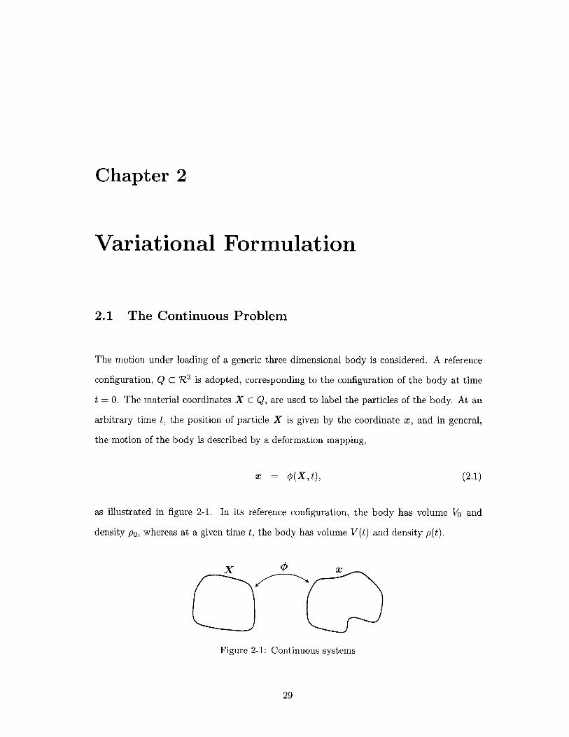
The motion under loading of a generic three dimensional body is considered. A reference
configuration, Q C R 3 is adopted, corresponding to the configuration of the body at time
t = 0. The material coordinates X E Q, are used to label the particles of the body. At an
arbitrary time t, the position of particle X is given by the coordinate x, and in general,
the motion of the body is described by a deformation mapping,
x = #(X, t), (2.1)
as illustrated in figure 2-1. In its reference configuration, the body has volume V and
density po, whereas at a given time t, the body has volume V(t) and density p(t).
Figure 2-1: Continuous systems
29
Page 30
2.2 The Action Integral for non-dissipative systems
For non-dissipative systems, both the internal and external forces in the system can be
derived from a potential, and the motion between times to = 0 and t, can be determine
from Hamilton's principle. To this end, a Lagrangian, L, is introduced, such that, £(x, d) =
K(+)-H(x) , where, K, denotes the kinetic energy, H is the potential energy and x = dx/dt
is the material velocity. The potential energy can be generally decomposed into an internal
elastic component, Hint, and a component accounting for the external conservative forces,
H1 ext. Thus, 1(x) = Hint(x) + Hext(x).
The action integral, S, is defined as the integral of the of the Lagrangian over the time
interval considered,
/tS = joLdt (2.2)
and Hamilton's principle states that the deformation mapping satisfying the equations of
motion can be obtained by making the action integral stationary with respect to all possible
deformation mappings which are compatible with the boundary conditions [15].
2.2.1 The Kinetic Energy, (K)
The kinetic energy of the body is a function of the velocity and can be written as,
K(e) = poi2dVo (2.3)
2.2.2 The Internal Potential Energy (Hint)
The internal potential energy depends on the constitutive relations of the materials in the
system. In this research hyperelastic Neo-Hookean materials are considered, which undergo
large deformations and displacements.
Let F be the deformation gradient tensor which can be written as,
Fi = -- V i,j = 1,.., 3aXj
30
Page 31
The relevant kinematic quantities associated with the deformation gradient are the right
Cauchy-Green tensor, C, the Jacobian, J, and the isochoric component of C, C, which
are given by,
C=FTF; J = det(F); C= J C.
For isotropic Neo-Hookean materials, the internal potential energy can be expressed in
terms of the Lame constant p, and the bulk modulus r, as
Hint(X) = 7rdV
tr(U)-3) (J - 1) dV. (2.4)
The above expression is well suited for compressible or nearly incompressible materials,
[72]. A detailed discussion for the treatment of incompressibility will be presented in a later
chapter.
The relevant stress measures and their relationship with energy can be expressed as follows
[72, 73]:
0ir(F) - P (2.5)aF
where P is the first Piola Kirchhoff (PK1) stress tensor. The PK1 stress and the true
Cauchy stress a are related as:
S= J- P FT (2.6)
The internal energy per unit volume can be split to deviatoric and Volumetric components
as follows:
7r(F) = 7rdev (F) + 7rvoi(F) (2.7)
7rdev (F) = ! {tr(O) - 3} (2.8)
7rvoi(F) = I (J - 1)2 (2.9)
31
Page 32
It can be added, that, from equation, 2.7, one could similarly split the PK1 and the Cauchy
stresses using the equations, 2.5, 2.6 , as follows:
87r(F) _ 87rdev(F) O7rvoi(F)OF OF OF
P = Pdev + Pvoi
(2.10)
(2.11)
(2.12)a = Odev + avol
where the Cauchy volumetric stress,
the unit matrix (I):
(avoi) is the hydrostatic pressure (p = ie(J - 1)) times
avoi = p I
and the other terms are:
Pvo1
Pdev
Odev
= pJF-T
= J- [F -F F-
3 _ b: I= pJ~3 [b -3I
2.2.3 The External Potential Energy (IHext)
The external potential energy includes the work done by the external body and surface
forces.
Hlext (X) = Jvf -xdVo - vf . x dS (2.13)
Here, fb are the body forces, f8 are the surface forces, and OV denotes the section of the
boundary, in the reference configuration, where the surface forces are applied.
32
Page 33
2.3 Discrete time integration
Consider now a sequence of timesteps tn+1 = tn + At, n = 0,1, ... , N, where for simplicity
a constant step size has been taken. The position of the body at each step is defined by a
mapping xn = #(X, tn). A variational algorithm is defined by a discrete sum integral,
N-1
S(xox1, ... , XN) S Ln,n+1(xn, xn+1) (2.14)n=O
where the discrete Lagrangian L approximates the integral of the continuum Lagrangian 'C
over a timestep, that is,
Ln,n+ 1 (xn, xn+1 ~ '(x,C ) di . (2.15)
Here, for simplicity, the case in which the Lagrangian is a function of x and x only, is
considered. The variable dependance, like that of pressure, will be considered later. There
are a number of ways in which the approximation (2.15) can be chosen, and, each one will
lead to a different time integration algorithm.
The stationary conditions of the discrete sum integral S with respect to a variation ov,
of the body position at time step n are now given by,
DnS[6vn] = D 2 Ln_1,n(xn_1,xn)[vn1 + D1Ln,n+1(xn,Kn+1)[6vn] = 0 V6v , (2.16)
where Di denotes directional derivative with respect to i-th variable. The above equation
represents the statement of equilibrium at step n and will enable the positions at step n + 1
to be evaluated in terms of positions at n - 1 and n. It will be shown in the next section
that regardless of the actual discrete Lagrangian chosen, the algorithms derived following
the above variational procedure will inherit the conservation properties of the continuum
system. Moreover, it is also shown in [5] that this type of algorithms are also simplectic.
As a simple example of the above variational integrators, consider first the standard case
of the commonly used central difference (or leap-frog) time integrator. This well-known
33
Page 34
scheme is arrived at by defining the discrete Lagrangian between two timesteps as,
2 M(vn+1/ 2 , vn+1/ 2) - At H(Xn) (2.17)
where the intermediate velocity is defined as vn+1/2 (xn+ - xn)/At and the mass bilinear
form is given by,
M(u, v) = (u - v) po dV . (2.18)
Substituting into equation (2.16) for the above discrete Lagrangian expression leads, after
some simple algebra, to the standard explicit central difference time integration scheme,
vn+1/2 -vn-1/2= F(bvn; Xn) - T(6vn; Xn)M ovn, (2.19)
where the external and internal forces are respectively,
F(6v; x,)
T(6v; Xn)
-DHext(xn)[6v]
Dflint(Xn)[ov1 . (2.20)
Remark For a uniform step size, identical explicit equations are in fact obtained if the
Lagrangian is approximated as,
Ln,n+1i(Xn, Xn+1)= t M(vn+1/2, vn+1/2) - At rI(xn+1)
At At AtLnn+ (Xn, xn+i) - 2 M(Vn±ii2,Vn±ii 2) - 2I7J(Xn) - 2-H(Xn±i)
However, for variable timestep size, only the last equation leads to the standard second
order leap-frog scheme.
A different scheme, namely the mid-point rule, can be derived from an incremental
34
or indeed,
(2.21)
(2.22)
Ln,n+1 (Xn, Xn+1)
Page 35
Lagrangian defined as,
AtLn,n+1 (xn, xn+1) = At M(vn+1/2, Vn+1/2) - At II(xn+1/2);
1Xn+1/2 = -(xn + xn+1)-2
(2.23)
Simple algebra shows that the resulting equilibrium equations are,
M Vn+1/2 ~ Vn-1/2) 1 {F(6vn; xn+1/2) + F(6v; xn-1/ 2 )
-T(Jvn; xn+1/ 2 ) - T(Vn; xn-1/ 2 )}
This is clearly an implicit scheme. It is well known, however, that for the linear case it is
unconditionally stable. Note also that the mid-point rule is more commonly written in a
one step for as,
M(V 7 Vn+ Vn) = F(6vn; xng) - T(vn; xn+);At
xn+1 = xn + -(vn + vn+1)-2(2.25)
Averaging this expression written between n and n + 1, and n - 1 and n, it is easy to show
that equation (2.24) is recovered.
2.4 Conservation of System Invariants
The conservation properties of the above variational algorithms are a consequence of the
invariance of the Lagrangian with respect to rigid body translation and rotations. This is
simply a particular case of Noether's Theorem, whereby the symmetries of the Lagrangian
lead to preserved quantities throughout the motion [15].
Consider the case of linear momentum first. This easily follows from the translational
invariance of the discrete Lagrangian in the absence of external forces. To show this note
first that if there are no external forces, then for any arbitrary constant vector a E R3,
Ln,n+1 (xn + a, xn+1 + a) = Ln,n+1(xn, xn+1) -
35
(2.24)
Page 36
Differentiating this expression gives,
DiLn,n+1(Xn,xn+1)[a] + D 2Ln,n+1(Xn,Xn+1)[a] = 0. (2.26)
But from the equilibrium equation (2.16), taking 6vn = a, the following relation is obtained:
D1Ln,n+1(Xn, xn+1)[a] = -D 2 Ln,n+1(Xn-1, xn)[a]
Substituting into (2.26) gives,
D 2Ln,n+I(xn, Xn+1)[a] = D2 Ln,n+1(Xn-1, Xn)[a] , (2.27)
which implies the preservation of the discrete linear momentum, G(xn, Xn+1), which is
defined as,
G(xn, Xn+1) 'a = D2Ln,n+1(XnKn+1)[a]
The case of angular momentum is similarly obtained from the invariance of the Lagrangian
with respect to rotations,
Ln,n+ 1(Rxn, Rxn+1) = Ln,n+1(XnXn+1) (2.28)
where R is an orthogonal rotation matrix. Differentiating this expression now gives,
DiLn,n+(xn, xn+1)[w x Xn] + D2Ln,n+l(XniXn+l)[w x Xn+1 = 0 Vw E Z72,29)
where w represents a small rotation (spin) vector associated with R which is arbitrary
since the choice of R, in (2.28), was also arbitrary. Again from (2.16) for the particular
case bvn = w x x, the following relation is obtained:
D1Ln,n+1(Xn, xn+1)[W x xn) = -D2Ln,n+1(xn-1, Xn)[w x x n,
36
Page 37
and substituting into equation (2.29) gives,
D2Ln,n+1(xniXn+1)[w x xn+1] = D2Ln,n+1(xn-1,xn)[w x xn] , (2.30)
which leads to the following definition of the discrete angular momentum H(xn, xn+1),
H(xn, xn+1) - w = D2Ln,n+l+(xn, xn+1)[w x xn+ 1] . (2.31)
Note that in order to define the discrete linear and angular momentum, only the depen-
dence of the Lagrangian on the geometry is relevant. In particular, when the Lagrangian
depends explicitly on geometry and the pressure, as in the next section, the above definitions
and derivations remain unaffected.
2.4.1 A simple example: System of Particles
As an illustration of the conservation laws derived above, consider the simple case of a system
of particles with masses ma for a = 1,.., M as shown in figure 2-2. The configuration at
Figure 2-2: A system of particles
time tn is given by a vector xn E R3M and xT = [x1,... , xa,.. .]. Consider the discrete
Lagrangian,
Ln,n+1(xn, Xn+ 1) = (2.32)E - mn+1/2 n+1/2 -At It(xn)a=1
where II represents some internal potential leading to particle interaction forces (which is
typically only a function of particle distances) and vn = (xn+1 - xa)/At. Both linear
37
Page 38
and angular momentum emerge from,
D 2 L(x,,xn+1)[vn+1] = mvi/ 2 -ovo 1i . (2.33)a
For instance, taking ov+ a, the standard definition of the linear momentum is recovered,
M
G(xn, xn+1) =1 m v/ 2 . (2.34)a=1
Taking nv1 w x xa 1 gives, after some trivial algebra, the angular momentum as
M
H(xaxn+1) = ma xa 1 x v . (2.35)a=1
The conservation property shown above, remains valid as long as the internal Potential
Energy II(xn) depends only on Xn.
2.5 Space-Time Discretization
Variational algorithms require a definition of a discrete action integral, which requires the
computation of the Lagrangian Integral between time steps tn and tn+1. To compute the
integral, a discrete space-time domain needs to be studied. In this section a brief description
of space-time discretization is presented. Computation of the Lagrangian Integral within
generic space-time volumes is explained by the example of triangular meshes.
In case of explicit schemes, the Potential Integral (II) is computed based on the variables
lying at time level tn. The Kinetic Energy Integral (K) depends on variables at both time
levels tn and tn+1 . To begin with, the computation of the Kinetic Energy Integral in a
single triangular element is described.
Figure 2-3, shows the typical space-time volume of a single triangle. The triangle abc,
and triangle abcn+1 enclose a prismatic space-time volume. This volume is further sub-
divided into three tetrahedra. The task is to compute the kinetic energy integral K within
each of the space-time-tetrahedra, and then sum each of the contributions to compute the
net integral within the space-time-prism. To do so, a generic space-time-tetrahedron(Fig.
38
Page 39
t n+1C b 4
3Ca
c/ b
t n
a X
Figure 2-3: The space-time-prism (left) and a generic space-time-tetrahedron (right).
2-3, (right)) is studied and the integral is computed as follows:
dzx = X(Xt) on,.+1 = - (2.36)
di
Where x is the position vector, X is the reference position vector and - is the total
derivative. Note here, that for the Kinetic Energy Integral, total derivatives of position
vectors, are considered. In the general case, any quantity (scalar or vector) would have
a similar treatment. First, a set of volume coordinates are introduced, analogous to the
area coordinates in case of triangles. The volume coordinates, given by ((1, 2, 3, (4) attain
values of 1 at their corresponding nodes and zero at other nodes, ie., (j is one at node i and
zero at all nodes j 5 i. Any function linear in X, Y, t, say F(X, Y, t), can be interpolated
within the tetrahedron, based on its nodal values Fa and shape functions Na = (a as
F(X,Y,t) = FaGa. The coordinate transform between (X,Y,t) and (4) can be
written as:
1 1 1 1 1 $
X X 1 X 2 X3 X4 (2.37)
Y Y1 Y2 Y3 Y4
t t1 t2 t3 t4 J 4J
39
Page 40
Inverting this relation gives:
1
6V0
6V1
6V2
6V3
6V 4
ai
a2
a3
a 4
b1
b2
b3
b4
C1
C2
C3
C4
1
X
Y
t
(2.38)
where ai's are the cofactor of the Xi elements in the transformation matrix. Similarly bi's
are the cofactors of the Y elements, ci's are the cofactors of the tj elements, and Vi's are
one sixth the cofactor of each unit element in the transformation matrix. Vo is the volume
of the tetrahedron given by:
1Vo =
1
X1
Y
ti
1
X 2
Y2
t22
1
X3
Y3
t 3
1
X 4
Y4
t 4
(2.39)
The derivatives of the function now can be written as, using chain rule:
dF _ F d 'dX 3 O~dXi (2.40)
where X = [1 X Y tIT. Thus, for the time gradients we can say:
dF _1 OF-- = 0 - - -- c 3 (2.41)
Now, since F is linearly interpolated, &F = F) which leads to a simple relation for the
40
4
Page 41
derivatives:
1 1 1 1
X1 X2 X3 X4
Y1 Y2 Y3 Y4
dF F1 F2 Fa F4dF 3 4 (2.42)
dt 1 1 1 1
X1 X2 X3 X4
Y1 Y2 Y3 Y4
t1 t 2 t 3 t 4
Similarly, assuming a linear interpolation of x in space and time, the velocity within the
tetrahedron is obtained as a ratio of two determinants:
1 1 1 1
X1 X2 X3 X4
Y1 Y2 Y3 Y4
X1 X2 X3 X4Vn,n+1 = (2.43)
1 1 1 1
X1 X2 X3 X4
Y1 Y 2 Y3 Y4
tl t 2 t3 t 4
Note here, that in the special case where two nodes of a given space-time-tetrahedron
have the same reference coordinate (implying the same point) then, the velocity in the
tetrahedron simply becomes (in this case assuming X1 = X 4 and Y1 = Y4):
=n,n+1 = (2.44)t 4 - tl
This simplification leads to a criteria for the choice of subdivision of any generic space-time
volume. One should choose to sub-divide a given space-time volume into as many tetrahedra
with common nodes as possible. This would lead to a simple velocity interpolation within
41
Page 42
the tetrahedron. Now the Kinetic Energy Integral K is computed within the space-time-
tetrahedron:
Kn,n+1 Po (vn,n+1 ' vn,n+1) dVo (2.45)
In the case of a tetrahedron with common nodes this volume, simply becomes:
Vo = A123 (t4 - t1 ) (2.46)
where A 123 is the area of the triangle with nodes 1,2 and 3.
1 1 11
A 1 2 3 = X 1 X 2 X3
2~~yY1 Y2 Y3
In the generic case the Kinetic Energy Integral Kn,n+1 would take the form:
1Kn,n+1 = Vo pPo (vn,n+1 - Vn,n+1) (2.47)
2
But in the case of a tetrahedron with common nodes, the Kinetic Energy Integral Kn,n+1
would take the simple form (m12 3 = PoA123):
Kn,n+1 (t4 - 1) 23 1 (vn,n+1 on,n+1) (2.48)
Now, revisiting the space-time-prism of the triangle (Fig. 2-3) it is observed, that it is
subdivided into three tetrahedra, each one of them have a common node. Hence, using the
above simplified relations, a very simple form of the Kinetic Energy Integral is obtained:
Kn"+I = 2ma'c n[(V+1/ 2 . Vna+1/2) + (v +1/ 2 - Vn+1/ 2 ) + (Vn+1/ 2 - Vn+ 1/2)] (2.49)
42
Page 43
Where mabe is the mass of the triangle abc and:
At = tn+1 tn
Vn+1/2 = n+1 n Vi = a, b, cAt
In case of a finite element mesh, the space-time volume of the entire mesh can be subdi-
vided into space-time-prisms corresponding to each element. Hence, the net Kinetic Energy
Integral obtained for the whole mesh would be:
At~aa a(.0Kn,n+1 = M -M Va+1/2 (2.50)
a
Where Ma is the lumped mass of each node(a) in the mesh. Similarly, the Potential Energy
Integral can be calculated as:
II, = ZriAe (2.51)e
Where ire is the potential energy per unit area in a given triangle. Thus, the net Lagrangian
of the entire mesh would be:
Ln,n+ = Kn,n+1 - At I
At M r n(.2M V+1/2 - +1/2 - At " (2.52)
a e
This leads to the discrete Lagrangian Integral of the Leap Frog method, as discussed in
section 2.3.
Hence, it is shown that the Leap Frog scheme, with lumped mass, can be interpreted
as an outcome of linear interpolations in space-time. In this section some generic space-
time discretization principles have been presented and used to develop the standard Leap
Frog time-marching scheme. The objective was to present the generic treatment of space-
time discretizations, which could be used in the further development of time-integration
algorithms.
43
Page 44
2.6 Standard finite element formulation
In the previous section, the discrete Kinetic Energy integral was obtained using a space-
time discretization. In this section, the variational formulation is studied along with spatial
discretization. A spatial discretization using linear elements (triangles in 2D and tetrahedra
in 3D) will be discussed. Based upon linear interpolation, the position vector x" in an
element e, can be written as:
" = NeXzn (2.53)e aa
where Na are linear shape functions within an element e. The action integral as discretized
in time in equation 2.14 now can be rewritten as:
S = S(x; a = 1,... , Nd; n =1,...,N)N
~ Ln,n+1 (z", on+1 ; a = 1, ... , N d) (2.54)n=O
where Nd are the number of nodes and N are the number of time steps. For the Leap Frog
Method, the Lagrangian within the time steps n and n + 1 can be written as:
Ln,n+1(", )n ' = Kn,n+11 At (Ienxt(x") + I,t(x")) (2.55)
The stationarity condition then becomes:
as - Lnn+1 + , 0 (2.56)
which leads to the relations between the derivatives of the Kinetic and Potential integrals
as:
OK n ,n+1 _ At - 9 " + t Kn_1,' =0 (2.57),9xn axn axn axn
Now, the internal Potential Energy and its derivative with respect to X" are studied. The
Potential Energy is a function of Xa at time level n. For convenience, the time index n is
44
Page 45
dropped for the rest of this section, therefore, xa implies xz unless mentioned otherwise.
In addition, the following index notation is used. Indices e, f are used to denote elements,
a, b are used to denote nodes, i, j, k, I are used to denote vector directions in the current
(spatial) configuration and I, J, K, L are used to denote the directions of vectors in the
reference (material) configuration. First, the deformation gradient within the element e, is
considered:
Ox ONee= = a (2.58)
where X is the position vector of the reference configuration. Note that since the shape
functions are linear in the element the gradients are constant within an element hence the
the deformation gradient is a constant within the element. Based on the Neo-Hookean
model, the potential energy can be written as:
II't(x) = [ Z re(Fe) dVeo (2.59)e e
7re(Fe) = r ev(Fe) + 7r",ol(Fe) (2.60)
7rdev (F*) = {tr(Oe) - 3} (2.61)
7r*,oi(Fe) = (Je - 1)2 (2.62)2
where
2
Je = det(Fe); Ce = FeTF*; be = FeFeT; Ue = Je 3 Ce;
Therefore, the derivative of potential energy wrt. x can be written as (using Eqn. 2.5)
Or(F) 07r (F) OF (2.63)Oxi OF Oxi
OF= P : - (2.64)
Oxi
45
Page 46
Further simplifying this in indicial notation, it leads to:
81r '9 kL0x7r PkL (2.65)
= PkL a i (2.66)8XLONe
= Pi L (2.67)
= PiL a FL (2.68)
Now, introducing a global index of a node as, b, such that it is the a'th node of element
e, (from connectivity) and revisiting equation, 2.59, one can express the derivative of the
Potential as:
8Hint(x) _8fr*(Fe)
M i nt ( X) 9 ( F e) d V (2 .6 9 )ax yo xa e(e,a)Eb e z
e Z AoIL Oa FLdV (2.70)(e, a) Eb fe Ox
Now, changing the reference volume V0 to V a current volume one can obtain:
B91int (X) MNe e -dPL a zL ~e e (2.71)(e,a)Eb *J
d
Inserting equation 2.6 into equation 2.71, one can obtain:
B9lint(x) - J 8N~ed8x y, oa o- dVe
(e,a)Eb V
Tb a (2.72)(e,a)Eb
where Tb are the internal tractions at node b along direction i, and the Tai are the elemental
internal tractions at a'th node of the element along direction i. Hence, it is shown that the
internal tractions, based on standard finite element, can be obtained, from the derivative of
the potential energy wrt. x. Similar to the internal Potential Energy, it can be shown that
46
Page 47
the external Potential Energy (2.13) would have similar derivatives:
811Iext (W Po Na- I dZe - v Na fzdSe(e,a)Eb (e,a)Eb JaVe
e-F = Fa(e,a)Eb
(2.73)
where ff are external surface force per unit area, and fb are the body forces per unit mass.
Further, from the Kinetic Energy integral obtained in the previous section, one could derive
expressions for its derivates:
Kn,n+1 (Xn, Xn+1)
v n+1/2
19Kn,n+1
Kn-_1,n (Xn_1, Xn)
2 MVn+1/2 - vn+1/ 2a
= (Xj (xi - X ai)atn+1 _ng
= Mbvbin+1/2
At~aVa
a= t Mn n-1/2-) a -/
= MbVbn-1/2
Using equation 2.57, we obtain the final discrete equation of motion as:
Kn,n+1 -AtM9 -int 49Kn 1 ,n
-At n+
Mb +1/2) =
Mb _vb+1/2 +v_1/2) - AtT = 0
At (Fnt - Ti)
which can be written in the vector form:
Mb V -vn 1/2 = At (Fb - Tb ) (2.76)
Thus, we obtain the time marching algorithm with the Central Difference Scheme, using
the spatial discretization of the standard linear element. The standard linear element de-
scribed above is commonly found in literature [74]. It was shown here that the standard
47
(2.74)
(2.75)
Page 48
element formulation is derived from a variational framework. This formulation performs
well, but it is known to be very stiff near incompressibility (volumetric locking), especially
for beam bending problems. A nodal element formulation has been developed [69], where
the deformation gradient tensor F is averaged at the nodes. This formulation is very well
suited for large strain explicit dynamic problems as it does not lock near incompressibility.
In the next section, the details of the averaged nodal element formulation are presented.
In addition, it will also be shown that the nodal element formulation is derived from a
variational formulation.
2.7 Averaged nodal element formulation
In this formulation, the interpolation of the position vectors is similar to the standard
element, but the deformation gradient tensor F is averaged at the nodes in the following
manner:
Fa eEa Fe/O (2.77)EeEa e
Similarly, the volumes are also averaged at the nodes:
V =(2.78)eEa
V"a EVe (2.79)eEa 77
where r is 3 for triangles and 4 for tetrahedra. The Jacobian at the nodes are then computed
by:
ja = a (2.80)V~a
48
Page 49
Now, the total internal Potential energy, for the averaged nodal element, can be written as:
II(x)
riev(Fa)
7rv"oi(Ja)
= Z(7re(Fa) + 7rao (ja)) Va
= {tr(Oa) - 31
= (Ja - 1)22
(2.81)
(2.82)
(2.83)
where,
Ca = FaTFa ; ba = FaFaT ; Ca = det(Ca) Cai
Differentiating the total internal potential wrt. a position vector at node b in the direction
k, (Xb), one can obtain:
z 7rdev(Fa)
a x
_ Orde,(Fa) 1
jFa -92
a a aOJac9r Ja) j
= j P" b
+ 7rvo (Ja) V)19xb
Now, rewriting the expressions for Fa and ja in equations 2.77 and 2.80, in the following
manner:
Fa = 1a eEa
a _
a eEa
I FeNadVoe o
eCNa~dV,
49
1911Oxk
&7rdev (F)
67rvoi (Ja)6xb
(2.84)
(2.85)
(2.86)
(2.87)
(2.88)
Page 50
Now, differentiating Fia, wrt. A we get:
1
a eEa
1
a e~a
1
a eEa
fL'O
Le'O
Jv'O
NadVe0a9xbk
8N* kg~Nb6ik NaedVeo
b~eN F jJ ik N a dVeO3x
which leads to:
&lrdev (F)
a eEa
Similarly, for the volumetric parts, one can write as:
aJ a
84b a eEa
a eEa
a eEa
a eEa
Le'OOJe ed e-NgdV
k4
oje N dVo
]VOJ F N~ dVeJaJFeyi aN e
,j Xj kgd
Je Fe- NbedV
6eNa ie 3
aVeb kj NaedVev xi
which leads to:
&7rvol (Ja)84b
pa a
IVe
Now, substituting 2.90 and 2.92 in 2.84 one can obtain:
b e-1
ea [Je Nj e
bFjeogiNaJ*- dVe +Ox3
PdevkJN) Fijj +(aEe
p a
eEa IVe
ZpaN)
N e6 kj*Ox,
Jki} dVe]
N dVe )Va
(2.93)
50
(2.89)
J &Ngpe6 ik NaedVeov'O aOx jJ
(2.90)
(2.91)
aN*b N dVeaXk
ail84b
(2.92)
Page 51
The final relation can be simply stated as:
a IT 8Ne&e adVe (2.94)
(e,a)EbJVe O
= Tb = [ Ta (2.95)
(e,a)Eb
(2.96)
where Tb are the global internal tractions at node b, and the Te are the internal elemental
tractions at element e, and node a, such that the a'th node of element e is the global node
b. Thus, the average nodal element is derived from a variational formulation. The standard
stresses (ae) (as mentioned in the previous section) and the average stress (de) (mentioned
above) in an element can be obtained as:
Je = det(Fe)
pe = K(Je - 1)
pe, = . Je~ Fe - F*e- F*e Fe-Pdev =3~~[ e
e = J- 1 PieFj + PeT (2.97)
e*= - J; 1 Pe FT + pel (2.98)
P e P a (F a)d~ev = dev (2.99)
aEe
= (2.100)aEe
where r7 is 3 for triangles and 4 for tetrahedra.
This formulation has been studied in [68, 69] and has been found to resolve the drawback
(excess stiff behaviour) of the standard element in case of near incompressible beam bending
type of problems. But in some cases [75], this develops some non-physical low-energy modes.
To stabilize this element a stabilized element, used in this research, is presented.
51
Page 52
2.8 Stabilized element
2.8.1 Stiffness stabilization
A stiffness stabilization using the finite element formulations in the previous sections has
been developed which addresses the problems encountered by the standard and average
nodal elements. In the previous sections, it has been shown that both formulations, are
variationally consistent. Hence, it can be shown that a linear combination of the two
element formulations would also be variationally consistent. A stabilized internal potential
energy comprising of linear combinations of standard and averaged nodal element can be
written as:
kstab = tIdev + adev (ldev - Ildev) + ,Vol + avoi(flvoi - vol) (2.101)
where the () quantities represent the average nodal stresses, and a terms are scalar param-
eters ranging from 0 to 1. Here a = 0 leads to the averaged nodal element, and a = 1 gives
the standard element formulation. From equation 2.97, 2.98 and 2.101 a stiffness stabilized
elemental stress can be calculated as follows:
dkstab = C ev + adev (Odev - &dev) + p + avol (P - P) I (2.102)
The choice of a parameters allow control in removing instabilities observed in standard and
averaged nodal formulations. The standard element has problems near incompressibility
where it shows volumetric locking, and in bending dominated problems it exhibits a very
stiff behaviour. The volumetric locking can be resolved by using the averaged nodal element.
To demonstrate the performance of the two formulations a beam bending case is chosen. A
vertical cantilever beam of length L = 10 m and width w = 1 m, is considered as shown in
the figure 2-4. The beam is fixed at the bottom and punched at the top half with a velocity
of vo = 2.0 m/s. The material properties of the beam are (E = 1.17 x 10 7 Pa, v = 0.49 and
p = 1.1 x 10³ kg/m 3 ). The solution was computed at t = 0.5s.
Figure 2-5 demonstrates how the averaged nodal element can be used to resolve the problems
52
Page 53
V0
L
Figure 2-4: A schematic of the beam bending case used to demonstrate the performance of
the standard and averaged nodal element.
P P1.343E000
M &8~70E400&8E0
I408E00I .10 080 - 1.2E+ 8 1 12E03800 37.000
8 -2.20E05 85 220E4000000E404 OOE00404
-i .00U-i100E05I -26.8005 -2.60E056 - 6
2 - 2 -
0 -
-2 0 2 4 6 -2 0 2 4 6x x
Figure 2-5: The standard element (left) shows excessive stiff behaviour undergoing less
deformation. The averaged nodal element (right) does not show any volumetric locking,undergoing larger deformations.
with the standard element.
On the other hand, the average nodal element, develops mechanisms in some 2D plane
strain cases [75]. To demonstrate the performance of the averaged nodal element, the same
beam bending case is considered, with a Poisson's ratio of v = 0.35. It is observed that
the averaged nodal element shows some hour-glass modes, where it undergoes unphysical
shear deformation (shear locking). To remedy this problem, the stabilized formulation,
mentioned above is used, with ade, = 1 and avo = 0, implying that it has the averaged
nodal pressures, and the deviatoric stresses of the standard element. The solutions obtained
from the two formulations are compared in figure 2-6.
This combination of (ade, = 1) and (a,i = 0) has been tried in simulation of plane
53
Page 54
Figure 2-6: The averaged nodal element shows shear locking (left) which is rectified by the
stabilized element (right)
strain problems without any apparent non-physical behaviour. It has to be noted, that for
all choices of adev and avoi, the element formulation remains variationally consistent.
2.8.2 Viscous stabilization
Time-integration methods are known to have dispersive errors which begin to corrupt the
solution over time. Especially in case of non-linear problems this issue becomes even more
severe. Due to the non-linearity, there is a strong coupling within the different modes in
the solution, which creates an exchange between the high frequency eigenmodes and low
frequency eigenmodes.
In the present case, variational methods have been presented, which ensure conservation
of linear and angular momentum. But no promise is made in terms of conservation of energy.
Although the energy is not conserved exactly, it has been found that the energy remains
bounded for long time integrations. But in case of severe non-linearities, there might be
some high frequency non-physical mechanism growing in the system, which needs to be
damped. Hence, there arises a need of a stabilizing viscous term which would damp, the
very high frequency modes, and yet would not dissipate the low frequency modes, which
would be of interest.
A dissipation term has been developed under the variational framework. The idea of
using viscous terms for stabilization is quite intuitive, but in order to maintain the conser-
54
p
10 1 0254067 00576405.06
5.005
22
0.'W
-2 0 2 4 6 +
6 14 2x
p1.345.06I ISE4(0
1 0 11.22E+6
5.405.063.805405
8 I2205.06026005
6 -420E+05
4
2
-2 0 2 4 6X
Page 55
vation property of the system, the viscous stabilization has to be momentum conserving.
In addition, the dissipation term has to be of a higher order in order to have minimal effect
on the net energy of the system. Similar to the development of the potential energy, where
a deformation gradient was used, here a velocity gradient is introduced:
d(=n-1/2) = (Vvn-1/ 2 + VTVn-1/ 2 ) (2.103)
1 __ 8x + Oxi
which can be split into deviatoric and volumetric parts as:
d = ddev + dvol (2.104)
dj = (dij - 6
d3 3
such that (dev = 0). For linear elements these velocity gradients are constant within the
element. Then, the velocity gradients are recovered at the nodes, and an average velocity
gradient is computed at the element by the expression:
\ f6,:eEa de/
d= Nea (2.105)
In case of linear triangular element, this simply becomes:
\ ( %:eEa e /
= d (2.106)a:aEe
Note here that the d is the value calculated at the centroid of the triangle. It shall be shown
later on that this will be sufficient for further calculations. Now a Dissipation Potential <I
55
Page 56
can be defined as:
(x-, on-1/2)
#(de)
#dev (ddev)
#voi (d ol)
= J#jk(de)dV
= #dev (ddev) + 4$01(d e1)
= Vdev (ddev : ddev)
1= voi(dvoi : dvol)
(2.107)
(2.108)
(2.109)
(2.110)
where Vdev and vvi are the viscosities. Similarly, a dissipation potential based on smoothed
rate of deformation gradients can be calculated as:
4(xn, on-1/2)
q5(d a
Odev (ev)
evoi (ao)
= Z (aa) a~= #(d"Vna
= dev(ddev) + Ovoli(d 0i)
= vdev(ddev : dev)
1 uoa :a2 -VV 0i(dV0 1 : d-l
(2.111)
(2.112)
(2.113)
(2.114)
So far, using the rate of deformation tensor, we have defined dissipation potentials which
are a function of Vn-1/2. In presence of viscosity, Hamilton's principle of stationary action
(2.56) modifies to:
DnS[6n]
iOs83 n
aen
= AtDa(D[vn}
= BAt(9Dxn, Vn-1/2)= At Oa-
n-1/2
(2.115)
(2.116)
Now, expressing the action integral in terms of Kinetic energy integral and potential energy
integrals as shown in 2.57 equation, we obtain:
(2.117)9Kn,n+1 _ A 1 - At + =At,n At(Xn, Vn-1/2)ax ax ax ax ovn-1/2
56
Page 57
Now, using the relation between on-1/2 and x, as:
a z~a - on__n ~1/ 2 At
aqVaon_1/2On_12 (2.118)
nx At
The equation 2.117 can be written as:
(9Kn,n+l At al" -art + K- 1 ,n -2 6'(xn, Vn-1/ 2 )Dgn Bn Ozn DOn BOa
Kn,n+1 (At + AtA) 9K_ 1 ", = 0 (2.119)ax ax a + a
In order to incorporate a higher order dissipation potential, the difference of standard
dissipation potential 4 and nodally averaged potential e is used. This leads to stabilization
of the internal energy in the following manner:
nstab(xn,vn-1/2) = Uktab(n) + At ((xn,vn-1/ 2 ) - 1(xn,vn-1/2))
(2.120)
Note that the additional terms are invariant to rigid body displacements and rotations,
hence they do not disturb the momentum conservation property of any variationally con-
sistent algorithm. Now the derivatives of the Dissipation Potentials are studied. First the
standard Dissipation Potential 4 is considered. The derivative of this potential with respect
to xb can be written as:
e:(e,a)Eb i
,90e 90e= dev + vol vee:(e,a)Eb %
=9de k1 -8(dvV}+{ O k1 V ] e (2.121)d ev a( d eq $ i9 #d o i e1 vo
e 19(ddev)E Oi S ~ vl$ k S
57
Page 58
Using equations 2.109 and 2.110 one can obtain:
8<pedev
a(ddev)ki
8(dv )e
= 2vdev (ddev)'el
Vvoi(dvoi) e
Now, considering only the deviatoric part:
{ OdaO(de)e } ye Z2Vdev(ddev)de )Vee
2vdev rddevbc ONa ( 6 ko6 ij + (5 io6 jE At axk 2
2vdev(ddev)ej Ne Ve
E At axj
3 (21
(2.124)
Now, considering the volumetric part:
8<1Oe, O(dvoj)' 1 } eZvvo ioi j Na(dvo)e
= zv~0 (dv0I41 ONi ___
e At axj 3
vvol(dvol), MeAt x3 Ve
Thus, the derivative of the standard dissipation potential becomes:
At-<04i ONa {2Vdev(ddev)?j ± tvi(dvoi)} yee:(e,a)Eb *x
Now, considering the averaged nodal dissipation potential:
dev a(ddev)fel
c' 8 (ddevdc )C e)
= 2vdev(ddev)ck 0
1q5901 O(dvol)c1 Qc+{O(dV0I)CkI I
8(o e a(d 0 o Ji+ voi(dvoi)kl k" Jj
58
Ee
(2.122)
(2.123)
} Ve(2.125)
(2.126)
(2.127)
Page 59
Now, considering only the deviatoric part:
2vdev (d)c (ddev)k d QcdE de ki OXb '
-d A( d e lVe) }frc
deEk (devkle c
(eEc.1(2.128)
where Qc = Eec Ve/ is the nodal volume at node c, and 1q is 3 for triangles and 4 for
tetrahedra. Further simplifying this equation leads to:
2Vdev (d
c IS (dd e v) ki
(eEc,(e,a)Eb
2 (dev k 9( e ( k I j + il~kj 6 ij6 kl V e
c (eEc,()Ea)EbL e (dd ev)k 2E
c{2l (dev 2 3 eEc,(e,a)Eb OxJ
1Oa2vdev ( ev) VAt Ox3(e,a)Eb v
Now, looking at the volumetric part:
eEc,(ea)Eb I
d e
cdeev)V~Ee I
(2.129)
2dev
(e,a)Eb 1
Vvo1(vo1) Cvi 0r4 } rc V (4v) c ( vo)elv }Pc(2.130)
59
Page 60
Now, simplifying in a similar manner shown in equation 2.129:
Z{-9t(dvoi)I
CC
,A{ (dvO1)kc
eEc,(ea)Eb
eEc,(e,a)Eb
(6ii kI
\\3 )/ (
(dvoi)Ve)
IN (ci r) }1 ex x
a kl e
eEc,(e,a)Eb x
At ec(yec I (eEc,(e,a)Eb
(e,a)Eb {($co1 V*
cEe 7
(2.131)E 1 z- { FVvoi(Voi)7} Ve(e,a)Eb
Thus, the derivative of the averaged nodal dissipation potential becomes:
At-8x~'
(2.132)89Ne'N {2Vdev(dev), +v vlij) ye
e:(e,a)Eb 3
Thus, based on equations 2.126 and 2.132, the stabilization of the Potential Energy, leads
to stabilized stresses in the elements, which can be calculated as:
avstab _ akstab + 2 Vdev (ddev - dev) + Vvol (dvol ~ i vol) (2.133)
Clearly the changes in the stresses are variationally consistent. The viscosities can be non-
dimensionalized based on mesh size as:
VdevpAX2
= fdev (2.134)
(2.135)pAx2Voc = voiAt
Thus, the amount of dissipation could be controlled by the non-dimensionalised parameters
Vdev and iDvol. A typical choice of 1, was effective to damp high frequency noise. To study
60
}
Page 61
the effect of such a dissipation term the following tests were conducted.
Patch Test
As a patch test, for the damping term, the stresses on a unit square plate, with the following
position and velocity field (x, v) was calculated.
x = f {ax + bX +cxY +dxX2 + xy2 + fxXY)
y = f(ay+byX+cyY+dyX2+eyy2+fyXY)
VX = f(ax + bxx + cxy + dx X2 + exy2 + fxxy)Atref
r = E (ay + byx + cyy + dyx 2 + eyy 2 + fYXy)Atref
(2.136)
where (ax, bX, cX, dx, ex, fx) and (ay, by, cy, dy, ey, fy) were non-zero constants. The average
stress computed as:
- e (0 vstab _ ,kstab) ,A(or =O (2.137)Ee e0
The average stabilized stresses (6-) were compared for different mesh sizes as shown in figure
2-7. In the above case, e = 0.1m, Atref = O.Ols and unit values for all the above constants
were chosen. The viscous parts of the stabilized stress which were the dissipation terms
only, showed a quadratic dependance on mesh size, and hence was a higher order term.
Beam Bending
Next the dynamic solution of cantilever beam was computed, exciting its first (lowest)
eigen-mode, for almost 20 cycles, to study the behaviour of the dissipation as shown in
figure 2-8. The beam was L = 20m long along the Y direction, and w = im wide along X
direction, hence it could be considered a slender beam. Using Euler-Bernoulli beam theory,
61
Page 62
Figure 2-7: Patch test showing the mesh dependancy of the viscous parts of the averagestabilized stresses.
the eigen-modes, are:
u(Y) = 6 {cos(kY) - cosh(kY)} + {-cos(L) - cosh(k)} {sin(kY) - sinh(kY)}}{sin(kL) + sinh(kL)}
(2.138)
where the eigenvalues are discrete values of kL, the lowest eigenvalue being kL = 1.875105,
and 6 was the initial deformation. Based on this, the initial deformation of the beam was
set as:
x = X+u (2.139)
U = U()(2.140)
-I'(Y) (X - (w2))
and the value of delta chosen was (6 = 0.001m). To test the dissipation term, the non-
dimensional terms chosen were (Ddev = voi = 0.01) and the solution and the energy
was monitored over the solution. The energy was assumed to be decaying in the following
62
-2 - - - - - -
-4 - -.-.-.-.
8 - ----- --- --
-3 -2.5 -2 -1.5 -1
logI(dx)
Page 63
--- 12elemn--- 2001e
1,0 -~;'
2000
.0.01
0.12 - . i . . I
B 10 15 20 25 30 34ime
manner:n
~I Worn
0.101 20 wlrm
C
W3 0.1
0.09
0.099r
0 B 10 1B 20 25 30 35 40lime
Figure 2-8: The energy history and the tip deflection for cantilever beam.
manner:
E(t) = Eoe-at
'9{ (t)
E )}Eo
= -a E(t)
= a
a = Cho (2.141)
where a would be the order of the energy decay. Tip deflection solutions were computed
upto a common time instant for different meshes, and the energy decay rate was computed
63
Page 64
from the energy history, using a regression relation as follows:
EOy = In )
~(EZt~yi) -- (Zti)(EZy;)= 0 a
(2.142)
(2.143)
Due to the decay nature, the absolute value of a (lal) was monitored, for different mesh
levels as shown in figure 2-9 The energy decay rates showed close to quadratic dependance
Figure 2-9: Energy decay rate variations with mesh size for beam bending.
(a: = 1.7) on mesh size for finer meshes 2-9, which was in accordance with the previous
observation in patch test. The the viscous stabilization is a high order dissipation term,
which becomes negligible in case of very fine meshes.
This dissipation term could be generically used in cases of explicit time integration, just
to filter out the high frequency noise generated due to the dispersion errors. It becomes
even more effective in case of non-linear problems. The non-dimensionalised parameters
Pde, and Dvo1 were typically chosen to be 1 or less.
64
-3 .... ...... .......... .. ..... ..
..... ......2...
~~. 3... ..... ...0. .. . .... .... . .. .... ..
..-. .. ... ... ... .... .. .. .... .. . ... . ...I. ..
.......... ... ...... .....' .-3.6.... ........
3 .6 ... ...... .. ...... . .. .... .. ...... .... ..
43..... 26 .. 26.. 24. 22.. 2.. ....... ...M J. .M. ..L .... ......... .... ... .. .. ... ...)I. ..
(E t?) - (E ti) (E ti)E
Page 65
Chapter 3
Mesh Adaptation
In this section, the previously mentioned variational formulation, is extended to mesh adap-
tation. Mesh adaptations which involve local mesh changes for 2D triangular meshes, are
considered. The following operations are formulated separately:
1. Diagonal Swapping.
2. Node Movement.
3. Edge Splitting.
4. Edge Collapsing.
Each of these operations is developed with the assumption that only one of these oper-
ations takes place between time level n and n + 1 on a local patch.
3.1 Diagonal Swapping
A discussion of diagonal swapping is presented, by studying a local patch of two trian-
gular elements abc and acd at time level tn, as shown in Fig. 3-1. The patch is time
marched to time level tn 1 where the common diagonal ac is swapped with the new diago-
nal bd, thus leading to two different element configurations, abd and bcd at time level tn+ 1.
The space-time volume thus formed, can be subdivided into five tetrahedra: (anbncnbn+1),
(ancndndn+1), (an+1bn+1dn+1an), (bn+1cn+1dn+1cn) and (ancnbn+1dn+1) as shown in the
65
Page 66
d
a
a
tn
tn+1
C
C
bFigure 3-1: The space-time volume for the diagonal swapping.
figure 3-1. Note that, the first four tetrahedra, have common nodes, hence the velocity
interpolation is simple. The velocity in the fifth(central) tetrahedra is computed by the full
expression, (as explained in chapter 2). Hence, the net Kinetic Energy Integral within the
space-time volume can be written as:
Kabcdn,n+1
abcdn+ 1 / 2
_At mabc b b At macd d d At mabd a a
t2 3 Vn+1/ 2 .Vn+1/2 + 2 3 on+1/2 - on+1/ 2 + 2 3 Vn+1/ 2 . n+1/2
At mbcd c At mabcd abcd abcd+2 n+1/2 n+1/2 3 n/+1 2 ' (+1/2
_ (macdx +1 + MabcdE+1 -bcd na + mabdXc (3.2)
Atmabcd
Using stationarity wrt. x, the equilibrium relations at tn are obtained as:
mabc b bx ±macd d 6m ab V n + 1/ 2 ' x b + m ac V n+ 1/ 2 ' n"
+ mabd va 1 / 2 + mbed abd ) a
(mbcd Vn+1/2 +mabd vnabcd 2 ' E3n 3 n' (3-3)
66
-D1 Knabc nd1[6*n]
Page 67
Similarly, using stationarity wrt. xn+1 , the equilibrium relations at tn 1 are obtained as:
-D 2Kiai[bXn+1] = aV_+1/2 -+1 + _cdn+1/2-
+ Mabc b Macd abc b
3 Vn+1/ 2 + 3 on+1/2 ' 64n
Macd d M abc acd d
+,3ne m+1/2 + 3 n+1/2 -m +1s
Thus, the finite element algorithm at step in is:
(3.4)
M," (vn+1/2
Md (n+1/2
- vn-1/2)
_n-1/2
SAt (Fn- T)
= t (Fn - T)
Note that as soon as the position of nodes b and d have been updated, using equations 3.5
and 3.6, it is possible to calculate vad/2 using 3.2 and this update of a and c:
Mn+Van+1/2 - Man"an-1/2 + mbed n+1/2a aa 3 'abcd
Mn+lvn++/2 - Mncn-1/2 + Mabd
A nCh3 fabi
And the finite element algorithm at step tn±1
an+1 (Van+3/2 -
Mn+1 (Vn+3/2 -
SAt (F - Ta)
= At (Fc - Tn*)
= At (Fn 1 -T
= At (F,4+ 1 - T+ 1 )
M n+1vn+3/2 - Mbn n+1/2b Vb bb
macd na1/23 Vabed
M n+1vn+3 /2 _ Mn n+1/2 mabc n+1/2d Vd d Vd - Vabed3
= At (Fb+1 -T+1
= At(F+ -+1
67
(3.5)
(3.6)
(3.7)
(3.8)
(3.9)
(3.10)
(3.11)
(3.12)
Page 68
The momentum within time step tn and tn+1 is (D2Ln,n+1):
= ~ Pn,n+1
Mn+1 n+1/2j V
Mnl n+1/ 2
j MVnj/+ (macd)Vabcd333 3n+1/2
Mnvn+1/ 2 +(abc vab|2S 3 + x Pn+1/2
- n~ X>Ixj± n x
for j = a or c,
for j =b,
for j = d.
Now another patch of elements as shown in Fig. 3-2, is considered to develop the algorithm
for edge-splitting. As shown in the figure, a patch of two triangles, abd and bcd, at time
level tn, is time marched to time level tn+1. The common edge bd is split at midpoint
d
a
a
tn+1
tn
Figure 3-2: The space-time volume for edge splitting.
e to form four child elements, abe, aed, bce and ecd, at time level tn+1. The space-time
68
Pn,n+1
Pn,n+1
(3.13)
(3.14)
3.2 Edge Splitting
(3.15)
Page 69
volume is now subdivided to five tetrahedra: (anbndn an+ 1), (bncndncn+1), (anc dndn+1),
(ancnbnbn+1 ), and (bndn an+1cn+1 ). Note that the first four tetrahedra have common nodes,
hence the velocity interpolation is simple. The fifth tetrahedra, is further subdivided into
four tetrahedra (as shown in red dotted lines in Fig. 3-2), each having a common node
as e. The point e and the mid point of b and d have the same reference coordinates,
(Xe = XbXd). Thus the Kinetic Energy Integral can be written as:
Kabcd At mabd a At mbcd cn,n+1 =2 3 Vn+1/ 2 - Vn+1/ 2 + 2 3 Vn+/2 - Vn+12
At mabe + mbce c c At mdae + mdec c c+ 2 3 Vn+/ 2 Vo+/ 2 ± 2 3 2 n+1/2
At+ mevn+1/2 'n+1/ 2
Me (mabd + Mbcd)me = a
Vn+ 1/ 2 - A n+1 2
(3.16)
(3.17)
(3.18)
Using stationarity wrt. x one can obtain:
-D1Knb+ 1 [6| = mabd a ' *a + mbd n+1/2 ' 64
mabe + mbce b -b mdae + mdecd 6xd+n+1/2 n 3 + n+1/2 n
+ 2 n+1/2 -64.d (3.19)
Thus, the update algorithm at step tn :
Ma (van+1/2 _ an-1/2)
Me" (vn+1/2 - vn-1/2)
= At (F- T)
= At (Fn - Tn)
M n+1 n+1/2 - M- Men+1/2Mb Vb Mbb 2 Ve
Mn1n+1/2 Mfn-1/2 me n+1/2d V d V d 2Ve
At (Fn - Tn)
= At (F- T)
69
(3.20)
(3.21)
(3.22)
(3.23)
Page 70
Choosing the velocity at the new node to be:
1 1 n+1/2 n+1/2) (3.24)
Thus a 2 x 2 system of equation is obtained, to be solved, to obtain the other velocities.
n+1 +1me
me
'Me n+1/2
M me Vb
M n+1 + ime n+1/2 I Mbn n+1/2 1 [ F - Tb!Vb +ItnT
M n+1/2 F -- T
(3.25)
The update at equations at n + 1 are
tn+1 is (D 2 Ln,n+1):
Pn,n+1
Pn,n+1
unchanged. The momentum within time step tn and
(3.26)= ZPn,n+l
M+1n+1/2 V
= zj+1 X Pnj,n+1
3.3 Node Movement
In order to initiate a study of node movement, the mapping of the present(spatial) con-
figuration to the reference(material) configuration, is revisited. An arbitrary intermediate
configuration((, r) is introduced, as shown in Fig. [3-3], as is typically done in the case of
Arbitrary Lagrangian and Eulerian formulation. The relations between the true and the
observed velocity fields can then be written in the following manner:
V - O4(X, t); v t = o(, t); V = (;
v= v - FV
The Kinetic Energy can then be written as:
Kn,n+1 (Xz, Xn+1) = Mn+1/2 I,n+1 - o,n+12
(3.28)
(3.29)
(3.30)
70
(3.27)
Page 71
Y
1l
y,
Figure 3-3: Understanding node movement with an intermediate mapping.
where:
Mj+1/2 (M + 1)I nI M
VnIni = Vn+1/2 - Fn +1/2
1Vn+1/ 2 = At (4+ 1 - Xn)
1V+ 1/2= At (n+ 1 - X)
fV NFndmFI = nd"fV Nyd
(3.31)
(3.32)
(3.33)
(3.34)
(3.35)
The deformation gradient Fn as used in equation 3.32 is evaluated at time level n in order
to make the update explicit. The corresponding equilibrium equations are (for any generic
node I, and its neighbouring nodes J):
M+V7,n+'1 21 M 1n,n+1 + At (F - TJ) (3.36)
71
X
Page 72
tn
t n+1
Figure 3-4: Space-time volume for node movement.
where:
VI,n+11
[(X±+1 - x ) - Fn (X+1 - XI)]
n+1/2
ZmJ (vf± 0 Vnn+1) J0 NyVoNydm
This expression remains explicit if the neighbouring J nodes remain fixed i.e. (Vnn+1+
in which case:
= (V0,n+1 V)n+) NyVoNydm
Provided that either I is an internal node or V' remains tangential to the reference boundary
['o. Thus for the node to be moved (I) the update step becomes:
V n,n+1 - M V__, = At (Fn - Tn)
And for the neighbouring nodes (J) the update step becomes:
(3.39)
Mn+1/2 Vnn+1 - Mn 1/2 vn_ 1 ,n = -At Q,n+1 + At (Fnf - Tn)
72
(3.37)
(3.38)
= 0)
- 0
NyVoNydm
(3.40)
(3.41)=(Vn,n+1 0Vn+1)Jv
Page 73
The momentum within time step t and tn+1 is (D2Ln,n+1):
Pn,n+1 = Pnj,n+1 (3.42)
Pn,n+1 = M 1 n+1/2 j
Hn,n+ = +1 x P ,n+1 (3.43)
3.4 Edge Collapsing
C q
P2 2
p1 q"Ir
Figure 3-5: Collapsing the edge ab to the point c.
Edge collapsing operation is approached by visualizing a generic patch of elements, as
shown in Fig. [3-5]. In the triangular element arb, the edge ab is wished to be collapsed,
leading to removal of the triangles arb and abs. The points a and b, belonging to time level
n, is substituted by the new point c at time level n + 1 as shown.
The space-time volume as shown in Fig. [3-6] is the volume over which the Lagrangian
is to be computed. To do so, the space-time volume is sub-divided into tetrahedra. There
are mainly three types of tetrahedra as shown in Fig. [3-7]. The first type (I) encloses the
volume arbsc. Then based on the surrounding nodes there are two types of tetrahedra, as
shown in Fig. [3-7]. The tetrahedra having a or b as one of the vertices, are labeled type
(II) and the ones having c as one of their vertices are labeled type (III). The location of the
73
Page 74
tn+1
tn
Figure 3-6: The space-time volume for Edge collapsing operation.
new node c is chosen to be a linear interpolation of the locations of nodes a, b and r.
XC+1
X = (o4 + 77 + (1 - ( - ?)
(3.44)
(3.45)
The Kinetic Energy Integral and the velocity interpolation within the tetrahedra of type
(I) can be written as follows:
At m"
2 3 n+1/ 2 -n+1/2
-marb ± abs
on+1 / 2
(3.46)
(3.47)At
Similarly the Kinetic Energy Integral and the velocity interpolation within the tetrahedra
of type (II) can be written as:
A t M n . ig2 m" n+1/2 n 1/2
n1
At
74
nn+1
g~ion+1/2
(3.48)
(3.49)
= Xn +nX (1 - (-)Xn
Page 75
Interior tetrahedrae
s Type I
a
Surrounding tetrahedra
Pt+W
Pi+1
P,.
P J+1
Type 11
' P
Figure 3-7: The subdivision of the space-time volume into different types of tetrahedra.
where the index gi is the overall index of all the neighbouring nodes, ordered as (gi =
r, qi, s, pi).
The velocity in the tetrahedra of type (III) is not straight forward, since there is no
common node in each tetrahedron. Hence the full expression of the velocity (described
previously) is used.
9494+1acvn+1 / 2
Kg+(III)n,n+1
_ A9j+1ac4 1 + Agiacn9+ Agic9i 1 +X 1 - Agia94+1Xa6Vg9+1ac
_ n gg+1c gigi+ giacS 9i n+1/2 n+1/2
(3.50)
(3.51)
This makes the algorithm very complex. In order to simplify the algorithm, an approxima-
75
P 41
a
Page 76
tion is made. The Kinetic Energy Integral from each of the tetrahedra, of type (III), are
added together, and the sum is expressed by the following approximation:
Z 2 = Vmn+1 n+1/2 ' Vn+1/2 (3.52)9i
V*+1/2 = At n+1 mc*x+1 + Amyt1 - m*xza - mxb] (3.53)
m = mn+ 1 _ (3.54)C C 3
Am 2 = m n+ 1 - mn (3.55)
m*, = m -_ , + Marcs (3.56)a a 3
m = m - mab + Mbascr (3.57)b b 3
Where Marc, and Mb, are the masses enclosed within arcs and bscr respectively. Note that
Am9 2 , m* and m* can be expressed as linear functions of ( and 7. The velocity vn 1 /2 is a
weighted average of the velocities of all the tetrahedra of type III as calculated in equation
3.50 In addition, since the neighbouring nodes are not moved, nor are any neighbouring
edge allowed to be collapsed, the mass mn+1 is known apriori. Thus the net Kinetic Energy
integral becomes:
Kn,n+1= Kn,n+1 + K, 1n+1 + Knn+1
At m" At
2 3 Vn+1/2 ' Vn+1/2 + 2 me 1 , n+1/2-+1/2At .1,9(
+ Z m"± gi1/ 2 n1/2 (3.58)
Using stationarity wrt. x, the equilibrium equations obtained at time level n are as follows:
(V9 n1/2 - m -1/2 = (Fe' - Trn') (3.59)
(1- - ) / + -+1/2 - -1/2 = At (Fi Tn)3 Vn+1/2 + m n'+1/2 - mVn-1/2 = At (Fn- Ta) (3.60)
3 Vnc+1/2 + ma Vn+1/2 - mb 1 na-1/2 = At (F- Ta) (3.2)
76
Page 77
Here, a new variable R' is introduced, where
Rn = mi v 112 + At (Fj - Tn)
Note that Rn is known apriori. Hence the set of equations, can be rewritten as:
(V g $ r)
( - -r on+1/23e
3
mi Vn+1/2
+ m. Vn+1/2
= Rgn
Vn+1/2 + m* Vn+ 1/2
n+1/2 + mb Vn+ 1 /2
(3.64)
(3.65)
(3.66)
(3.67)
Note here that Eqn. 3.64 is fully explicit, hence, x for all gi except r are known. Now
revisiting Eqn. 3.53 one can rewrite the expression for vn,+1/ 2 using Eqn. 3.65 as:
= Sm(, r7)Vn+1/2 + W(, r) (3.68)
At n+1W(~, ?7) [ZAmyiz,- - max - m* b
(3.69)
where,
AtRnrr
m" n= mab
3mn+1m
(V gj 4 r)
(gi = r)
3m*mm
m r " (Amr(1mab
= So+ St+S1 + S2 2 22 + S j(Z2 (3.70)
Note that the vector coefficients (Wo, We, W.) and the scalar coefficients (So, S', S1, S, S, S )
are known apriori. Using Eqn. 3.68 in Eqns. 3.66 & 3.67 the two equations are rewritten
77
(V j = gi, a, b) (3.63)
n+ 1
= Wo+( Wg +r; W7
+ m*,c Im z
Page 78
as:
Ka((, 7) Vn+11 2 + m*(Cr) W(, 7r) = (3.71)
Kb((, r) Vn+1/ 2 + m (Cr) W(,r) = (3.72)
where,
Ka(, r) = - + m *,) Sm(,r) (3.73)3 aMn
Kb(, 77) = r7 + m(, 77) Sm((, 77) (3.74)3 b
Now, eliminating Vn+1/ 2 from both the above equation, the following equations are obtained:
c ~Ra - m* ((, r1) W(( ln+1/2 = K(C, 77 )(375)
f (, r7) = (R m* W)+ (m W-R) = 0 (3.76)Ka n ab n
Thus, a simple vector equation (3.76) is obtained, which is used to determine the scalars (
and 77 by which, the position of the new node c is determined. This is a coupled quadratic
equation which is solved by iteration. A simple Newton iteration leads to quadratic con-
vergence. This leads to the position of the new node (X,+ 1 ) to be a solution of the local
equilibrium. Edge ab is collapsed only if the node c lies within the area included by all the
surrounding nodes gi.
Once the position of the node c is obtained, the velocity updates are obtained through
simple explicit equations mentioned above (3.75,3.68 and 3.65). The position updates are
obtained by the Eqns. 3.47 & 3.49. The momentum conserved in this time-step is of the
78
Page 79
form:
Pn,n+1 = Pn,n+1 (3.77)
J 3+1/2 Am3 vn+1 /2 , for j = gipn,n+1 = M 3 + * (3.78)
mn+ m +/ + +1 - )n+1/2, for j = ci Mab n)+ 1/2+ MnI 3 V 12
Hn,n+1 = zn$ X+1 Pn,n+1 (3.79)
Similar to the previous time-step, using stationarity wrt. Xn+1, the equilibrium equations
for the next time step tn+1 are obtained. The final update equations are:
m"' 1v"/ - m9,v, 2 - Am *,+~1/2 = At (Fngl - Tngi 1 ) (3.80)
1 m"n+1n+1/2 - 3mabn+1/2 - (mn+1 - 3 )vn+1/2 = At (Fn s 1 - T w) (3.81)
3.5 Implementation
With the mesh adaptation procedures, explained, so far, an effective mesh-adaptive solver
can be implemented which is momentum conserving. In order to develop a mesh adaptive
solver, a suitable mesh adaptation, criteria based on error estimates was used. In this
section details of mesh adaptation criteria and other implementation details are presented.
3.5.1 Error Estimate
There are various error estimates used in the literature based on gradients or functional
outputs or from residues or from constitutive relations. Due to the local mesh operations,
described in the previous section, a particular gradient-type error estimate was used, based
on a recovered solution in a local patch. The error-estimate described by Zienkiewicz and
Zhu,[46, 47]y commonly known as Z2 error-estimate was used. This error estimate, although
described for linear material properties has been extended for non-linear materials, and has
been found quite effective in the present genre of problems.
To begin with the description of the error-estimate, the computed solution on an 'h'
79
Page 80
level grid can be written as:
Xh = NX (3.82)
where i are the nodal positions vectors and N are the shape functions. The stresses in the
elements can then be computed from the the position vectors through a non-linear relation
as:
ah = a(Xh) (3.83)
This stress Oh, is the stress tensor, at each element. From this stress, the Z2 error suggests,
a recovered stress, such that:
a* = Na* (3.84)
where a* are nodal values of the stresses, which satisfy:
j NT (a* - h) dQ = 0 (3.85)
which leads to a simple evaluation of a* as follows:
.* = 0 (3.86)fn N NdQ
Note here that the stresses can be recovered at each element from the above relation, in
case of linear triangular elements, as:
S ea (3.87)aeEa Ae
o* Ne&*e*= N**a(3.88)
This involves lumping of the fn NTNdf2 matrix in the denominator. Now from this recov-
ered stress at each element, an error-norm is suggested, to get a measure of a local and the
80
Page 81
global norm.
(N 1/2IIEIIR 2III (3.89)
e=1
IeI|' = {Le - ah) : (c* - Uh) d} (3.90)
It has been shown in the papers by Zienkiewicz and Zhu [46, 47] that such a recovered stress
has super-convergence with mesh size, and the error-estimate shown above has quadratic
convergence with mesh size. In those works, examples were chosen from linear problems,
where as the present research involves non-linear problems. In addition, due to the lumping
of the fo Ng'Ndf2 matrix, the super-convergence of the recovered stresses with mesh size
is also not guaranteed. Hence to test the behaviour of the error-estimate, a punch problem
was used as a test case. The unit thickness square plate with material properties (E = 1.7 x
107 Pa, V = 0.450 and p = 1.1 x 10³ kg/m 3 ), and the applied punch velocity Vpunch = 2m/s.,
was chosen, as shown in figure 3-8. For a uniform mesh, error growth and instantaneous
Vpunch
Figure 3-8: A schematic of the punch test case.
error behaviour was studied. Figures (3-9,3-10 and 3-11) we see that such local errors do
predict the sensitive regions of the solutions, which in this case is a corner where stress
concentration takes place. To study the behaviour of the global norm in a dynamic sense,
the error growth is studied as shown in figure 3-12: Error studied at a time instant wrt.
different mesh size, is shown in the next figure 3-13, where in, quadratic convergence in error-
81
Page 82
1
0.8
0.6
0.4
0.2
0
ESxx
1200
04000-4004800-1200-1600
0.80 0.2 0.4 0.6x
Figure 3-9: Error in stresses oxx.
ESxy10012008004000
1 -- 400-00-1200
0.8 --- 16000.8
0.6 -
0.4 -
0.2
0
0 0.2 0.4 0.6 0.8 1 1.2x
Figure 3-10: Error in stress axy.
estimate is shown. This was in agreement to the observations described by Zienkiewicz and
Zhu [46, 47], even in the case of non-linear problems.
82
1 1.2
Page 83
1
0.8
0.6
0.4
0.2
0
ESyy150010005000
-1000-1500-2000-2500-3000
0 0.2 0.4 0.6x
Figure 3-11: Error in stress a-yy.
28a Elem128 Ebm
8.00E+03 1
6.OOE+03 -
4.00E+03 -
2.00E+03 -
0.00E+00 -
0 0.1 0.2 0.3time
0.8 1 1.2
Figure 3-12: Error norm in stress ||e|R at different instants in time for different mesh size.
3.5.2 Adaptation Criteria
Based on the Z2 Error-Estimate, a simple adaptation criteria is implemented. We define a
scalar OR as:
e~ Il-III\\ ||R (3.91)
83
Page 84
Figure 3-13: Mesh size dependence of Error norm in stress ||&-|R
And then elements with relatively higher values of theta were chosen for adaptation, typ-
ically (Ve OR > C9R..), where C was an input parameter typically chosen in the range
(0.5 < C < 1.0).
Once the element was chosen, the edge length ratios (77) were obtained by (7i = ,
where li is the length of the ith edge, which varied from 0 to 1. Edge length ratio, close
to zero or one, indicated mesh-skewness, which were collapsed or split or swapped. Edges
with edge ratios close to 0 say (7i < 0.3), were collapsed. Edges with edge ratios closer to
1 say (qi > 0.7) or higher were swapped or split. In case of node movement, a local patch
of nodes were considered, and the average (centroid) and the deviation of the node from
the average was calculated. For higher deviation values, the node was moved towards the
centroid.
The adaptation sequence used for all the operations, has been simple. Most mesh adap-
tation involved two timesteps (t, -+ tn+1) and (tn+1 -+ tn+ 2). Only one operation was
attempted within each pair of timesteps. Adaptation was attempted after constant inter-
vals (number of time-steps). Diagonal swapping, node movement, edge-splitting and edge-
collapsing were attempted in this sequence at every subsequent (or alternate) timestep pair.
Depending on the need, the lowest (finest) hierarchical level of the grid was prescribed, in
order to prevent over-refinement. The zero'th hierarchical level elements were not removed,
84
4-
3.8
3.6-
3.4
3.2
3
1.4 -1.3 -1.2 -1.1 -1 -0.9 -0.8
og10(h)
Page 85
in order to prevent over-coarsening.
Now some examples using mesh adaptation procedures described so far, are presented
in the next section.
3.6 Mesh Adaptation Examples
3.6.1 Spinning Plate
A unit thickness square plate, spinning without any constraint, was considered as a test case
to illustrate the conservation properties of the proposed mesh adaptation procedures. The
plate was made out of nearly incompressible rubber material with material properties, viz.,
Youngs Modulus E = 1.7 x 10⁷ Pa, Poisson's ratio v = 0.45 and density p = 1.1 x 10³ kg/m 3.
The plate rotated at 1000 RPM. The plate was meshed with 200 equal linear triangular
elements as shown in Figure 3-14 (left) which also shows the pressure distribution at a
given instant (right). The simulation was conducted using a mesh-adaptive solver, using
all the above mentioned, adaptation procedures viz., diagonal swapping, node movement,
edge-splitting and edge collapsing. A simple mesh adaptation criteria based on the the mesh
edge skewness and elemental stress was used. Figure 3-14, demonstrates how the mesh was
refined where the mesh skewness and stresses were relatively larger. The center of mass was
P p4006.04 *40064+04-200.06 .6.73E406
-3.4+0 QA.40
1.2- -. a0605 1.2 - 40-a2020 --7606406 *4 106.06
1 4006.05 1 U-7,206E0641.04E406 43DE405*1 166406 4406405
0.8 .326.06 0.8 1 . 066.1.41t406 -1.16606-1.606406 -127606
0.8 -174640 0.6 -1.366406
0.4 0.4
0.2 -0.2
0 -
0-0.2 -- 0.2
-0.2 0 0.2 0.4 0.8 0.8 1 1'2 1 4 -02 0 0.2 0.4 0.6 0.8 1 1'2 14x x
Figure 3-14: A Spinning plate simulation with adaptation.
initially at X = 0.5, Y = 0.5, and as a consequence of conservation of linear momentum
Pn,n+1, the center of mass would be expected to remain at the same location. Although due
85
Page 86
to node movement, some minor fluctuation in the center of mass location could be expected.
The angular momentum Hn,n+1 would also be expected to remain constant during the time
integration.
Figure 3-15: Linear and angular momentum history
As expected, the momentum remains conserved exactly, throughout the simulation as
shown in Figure 3-15. The momentum calculated in each step was based on the Pnn+1
and H,n+1 expressions described in each of of the adaptation procedures previously. There
x2MI
y4-,CMI
II
0.8
0.7
0.6
0.5
0.4
03
02
0. .0 0 0.05 0.1 0.15 0.2 0.25
Figure 3-16: Location of center of mass.
was no noticeable change in the center of mass, as shown in Figure 3-16, which was also
expected. Figure 3-17 shows the energy history during the simulation. Although there are
slight fluctuations in the energy behaviour, initially, but with time, the energy remains more
or less bounded, with no significant rise or dissipation as shown in Figure 3-17.
86
............. -YMom
An& MmL.25000A
20000 -
15000-
1000
0
5000
0
-50%05 0 0.05 0.1 0.15 0.2 0.25
Page 87
1.2
1
0.8
0.6
0.4
0.2
0
.............Knetic Ea t- - PoaimtIEherg____Towa Enw
00.05 0.1 5 02 065
Figure 3-17: Energy history.
450
400
350
~0300250
200
150
z 100 -
so1
5 0 1 - . I -
0 5000 10000 15000 20000dMe steps
Figure 3-18: Mesh Adaptation history.
Figure 3-18, shows the adaptation history, with the number of operations conducted
and the total number of nodes and elements during the course of adaptation.
3.6.2 An oscillating ring
A unit thickness circular ring, made up of nearly incompressible material (E = 1.0 Pa,
v = 0.450 and p = 1.0 kg/m 3 ) is initially stretched and let to oscillate freely. This was
chosen as another test case to study the momentum behaviour under large stretching and
free oscillation. The ring was meshed using 576 triangular elements initially. At t = 0,
the mesh is deformed as shown in Figure 3-19. The ring is let free to oscillate there after.
Time integration was performed using the mesh-adaptative procedures, using only diagonal
87
Page 88
swapping and node movement. The purpose, here was to address mesh-skewness, and hence
no refinement and coarsening was conducted.
1.5 - xO 1.5 - x0
1 05045 [7 045
1 0.25 10215
0.5 7-0.75 0.5 7-0.750-095 -0.95
0 -0
05 -- 0.57
-1 -1 -
__1_5 ___._._.__._._.__._._.__._ A.1 -15 ..,.,,.-15 -1 05 0 05 1 15 -1.5 1 05 0 0.5 15
X X
Figure 3-19: A circular ring(left) is initially stretched(right) and let to oscillate freely.
Figure 3-20 shows two arbitrary instances of the ring demonstrating multiple wave
modes. Node movement can not be seen in the spatial configuration, but diagonal swaps
can be clearly seen. Also to be noticed is that the ring remains centered at the same point
Mesh adaptation was based on mesh skewness.
1.5 - x0 1.5 - X0
00.5 0 85
S0.65 0655 - 0 45
1 -2 -1 - 2
-0.05 -050.15 1 -0.25
-0.35 -0.35-0.55 -0.55
0.5 7-075 0.5 - -0.75-0 95 -0005
0 -0
05 - 5
-1.5 -1 -05 0 05 1 1.5 -15 -1 -0.5 0 05 1 15X X
Figure 3-20: Deformation at intermediate step with adaptation.
Figure 3-21 demonstrates conservation of linear and angular momentum.
3.6.3 A Tensile test case
Next, a tensile test case is presented. This test case was chosen to observe the momentum
behaviour in presence of external forces. In order to demonstrate the exact conservation of
linear and angular momentum, a modified measure of momentum is calculated.
88
Page 89
0.2
0.15.
0.1
0.05
O
405
4.1
-0.15
402 10 . I ,o W J
Figure 3-21: The momentum history for the oscillating ring.
Modified Momentum
The measure of the modified momentum can be computed from the basic idea of measuring
the momentum, in absence of external forces. Subtracting the effects of external forces from
the actual momentum, the following measure is devised.
Pn,n+1 = Pn,n+1 - P ( PogndVo) + Ra+1 Atn (3.92)0 aEr
n =,n+1 Hn,n+1 - [( Pox x gndV) + Z xn x Ra+1 Atn (3.93)0 .aEr
Where gn is the external acceleration, (say gravity etc.), and is computed, like the external
forces are computed, (actually external force vector could also be used), while the external
nodal forces, R4+1 can be obtained while applying the boundary conditions. The modified
momentum thus obtained is expected to remain conserved, in spite of presence of external
forces.
In the Figure 3-22 a square steel plate, with material properties (E = 2.1 x 10¹⁰ Pa,
v = 0.3 and p = 7 x 10³ kg/m 3 ) is pulled rapidly by vpunl = 40m/s at its top surface, and
reaches thrice its length within 0.05seconds.
Mesh adaptation was employed in the simulation, and the net momentum was conserved as
is shown in Figure 3-23.
89
Page 90
-1 -. 5 0 0.5 1 1.5 2X
Figure 3-22: A Tensile test specimen (left) pulled to thrice its length (right).
Figure 3-23: The Modified Momentum history for the Tensile test
3.6.4 A Punch test
Similar to the tensile test case another test case as that of a punching problem was con-
sidered. A flat square plate of unit length was constrained from the bottom and sides and
punched into the top half with a prescribed punch velocity (vpunch = 2 m/s) as shown in
Figure 3-24. Here a nearly incompressible rubber plate was chosen with material properties,
(E = 1.7 x 10 7 Pa, v = 0.450 and p = 1.1 x 10 3 kg/m 3 ). The deformed configuration at
t = 0.25s is shown in Figure 3-25.
The Modified momentum remains conserved as shown in the figure 3-26.
3.6.5 Plate Impact
In this example a plate impacting a rigid wall is shown. The Taylor Bar impact (TBI)
is a standard benchmark in rapid dynamics problems involving large deformations. The
90
[4-L.44-2505.460
-4605.4
-17 005400
3
2.5
2
1.5
1
0.5
0
3
2.5
2
51.5
1
0.5
0
P-146E+10-1.20+10
-1.505.1-160410-12M10-246+10-2.045.1-2.62E.10
*U
0 1
0.4
0.2
0-
-0.2
-0.4
.J01 0 0.01 02 0.03 0.04 0.05 000
2
Page 91
Vpunch
7C
Figure 3-24: A schematic figure of the punch test case, showing boundary conditions.
0.8
0.6
> 0.4
0.2
0
P
7 60E406
5.40E405
4.20E+053.00E+061606E+08
-4.20E+06,
':0.2 0 0.2 0.4 0.6 0.8 1 1.2
Figure 3-25: Mesh adaptation for a punch problem.
standard TBI problem involves plastic deformations of a rod, impacting a rigid wall. In
this case a plate impacting a rigid wall is considered. Since only hyperelastic materials have
been considered in this thesis, a modified TBI problem is presented where the constitutive
relations are based on hyperelastic behaviour.
In this case, a plate of length L = 32.4mm and width w = 6.4mm impacts the rigid
wall with a velocity of 227m/s. Using symmetry, only half of the plate is considered with
appropriate boundary conditions, as shown in figure 3-27 The material properties of the
plate were (E = 5.85 x 10 8 Pa, v = 0.495, p = 8930 kg/m 3 ). The plate was discretized
91
Page 92
........... .. LM ,M.
Ang. Mom
0.5-
0-
-0.5
-1-
-0.05 0 0.05 0.1 0.15 0.2 0.25 0.3Time
Figure 3-26: The Modified Momentum history for the punch Problem
W
Vj L L
w/2
Figure 3-27: Schematic diagram of the plate impact problem.
using 200 elements and the solution was computed for 194pts. Figures 3-28 to 3-31 show
the solution of the deformed plate at various time instants. The mesh gets refined in the
regions of high error (Z 2 error) and high mesh skewness. Figure 3-31 shows adaptation
near the contact where the mesh undergoes the most skewness. The plate touches the the
wall at 14 Is. In figure 3-28 the plate is shown to collide with the rigid wall within the
first 30 ps where the body distorts at the contact of the wall. With further motion untill
60 ps, the mesh distorts inside, where the mesh is adapted. All the kinetic energy of the
plate is almost converted to internal potential energy by 90 Is as shown in figure 3-33 and
3-29. After 120 pis the plate springs back in the opposite direction (reaction). The plate
springs back untill 150 p.s, where it undergoes large necking type of deformation, where
meshes are adapted as shown in figure 3-30. At roughly 180 pis, the plate leaves the rigid
92
Page 93
Figure 3-28: The plate at t = 30 ts (left) and t = 60 ps (right).
Figure 3-29: The plate at t = 90 ps (left) and t =120 ps (right).
P
2.5024092,222400
0.045 - 188E0 0.0451.542409
0.04 120E400 0.04
0.035 1802.08 0.035
0.03 0.03-118E408
0.025 0.025
0.02 0.02
0.015 0.015
0.01 0.01
0.005 0.005
0 0
.01 0 0.01 0.02 0.03 -0.01 0 0.01 0.02 0.02x x
Figure 3-30: The plate at t = 150 ps (left) and t = 180 ps (right).
93
P
0.045 222E.00184400
0.04 20
0.025 -190+0882.GE00
0.03 -002E408-8.402408
0.025
0.02
0.015
0.01L
0.005
0
-0.01 0 0.01 0.02 0.03x
Page 94
wall (bounce-off motion).
Figure 3-31:mesh in the
Deformed configuration of the plate at treference configuration (right).
= 194 ps (left) and the corresponding
The modified momentum in this case remained constant, as shown in figure 3-32.
Figure 3-32: Modified Momentum history of the plate
Figure 3-33 shows the energy history. The energy has a slight decay over time due to
viscous stabilization. The remeshing operations introduce small energy spikes, which are
stabilized.
94
P2 90E409
2.22E4090.045 1 W8E.O
1.54E+090.04 -2E4O
S SCEoCSo52oss
0.035 -1,80E+08-1.60E+06
0.03 405.E0
0.025
0.02
0.01
0.005
01
-001 0 001 0.02 0.03x
PI 2 *9O092.22E4092 26E+09
0.03 154E+09120E+09
0.025 520E+6
-1 OOE+08400OE40
0.02 -
0.01
0.005
00 0.01 0.02
xo
-.-- -. XMom.- -- YMom.
Ang. Mom.50
0
-50
-100
-150
-200-
1 -04 0 0.0001 0.0002 0.0003Time
Page 95
.............. Kinetic EnergyPotential EnergyTotal Energy
1.2
0.8
0.6-
0.4 -
0.2 -
0
0-t -04 0 0.0001 0.0002 0.0003Time
Figure 3-33: The Energy history.
3.7 Concluding Remarks
In this chapter variationally consistent time updates for local topological changes have been
developed. The methods have been formulated using the space-time discretization described
in chapter 2. These updates have been implemented in tandem to develop a simple mesh
adaptation algorithm. A simple mesh adaptive criteria based on the Z 2 error-estimate has
been used. The mesh adaptation algorithm thus obtained, is shown to conserve linear and
angular momentum. In cases of external forces, a modified momentum is used to demon-
strate the conservation of momentum. Simple cases of rapid dynamics have been shown to
demonstrate the application of such methods. The existing adaptive procedures are explicit,
and cause no significant extra expense over the standard explicit (central difference) scheme.
Clearly, further work is required to augment the use of the algorithm to more complicated
problems, where severe mesh distortions are encountered. Better mesh adaptation criteria
would be required, to make the adaptation more effective.
95
Page 97
Chapter 4
The Fractional time-step method
4.1 The Mixed Formulation
The internal potential energy depends on the constitutive relations of the materials in the
system. In this research hyperelastic Neo-Hookean materials, undergoing large deformations
and displacements, have been considered. The internal potential energy has been expressed
in terms of displacements in chapter 2.
The expression for internal potential energy (Eqn. 2.4) is well suited for compressible or
nearly incompressible materials. However, when the material approaches incompressibility,
the bulk modulus, r., becomes very large and this causes IIt(x), in (2.4), to be unbounded
for all motions not satisfying J = 1. This is a constraint on the allowable deformations
which, in practice, is difficult to enforce a priori. A more suitable formulation which permits
computation of general motions is obtained by introducing the constraint, J = 1, through
a Lagrange multiplier. It turns out that, it is actually possible to reformulate the internal
potential energy, by introducing an additional pressure variable in such a manner that a
formulation which is valid for both compressible and incompressible materials is obtained.
This is generally referred to as the mixed formulation which uses pressure as a separate
degree of freedom. In the compressible case, the pressure can be determined from the
volumetric change as p = (J- 1), whereas in the incompressible limit, the pressure becomes
a Lagrange multiplier and thus a separate variable, which enforces J = 1. The mixed
97
Page 98
formulation can be written as:
flint(x, p) = Hiso(x) + flvoi(xp) , (4.1)
where,
Hiso(x) = (tr(a) - 3)dVo , (4.2)
and,
Hvoi(x,p) = ]p(J - 1)dVo - dVo . (4.3)/V /V 2 r
For compressible materials, the constitutive equation relating the volumetric changes and
the pressure is recovered by setting the variation of 1 voi with respect to p equal to zero. Thus
the form (4.1-4.3) of the internal potential function, has the property that it is equivalent
to the irreducible form (2.4), but as the material becomes incompressible, the second term
in Hvoi disappears and only the constraint times the Lagrange multiplier, p, remains. As
expected, for incompressible materials, Hy,1 -+ 0, and Iliso -> Hint. It is clear that when
the form (4.1-4.3), is adopted, for the internal potential energy, the Lagrangian will also
depend on the pressure, that is (x, x,p), and that the solution will need to be determined
by requiring stationarity of the action integral, (2.2), with respect to x and p.
4.2 Fractional Step Variational Formulation
Here, the time integration algorithms, introduced in the previous section, is extended to
the case in which the volumetric internal potential energy, and in turn the Lagrangian,
is expressed in terms of the configuration x, and the pressure, p, as given by equations
(4.1-4.3).
98
Page 99
Consider the following discrete Lagrangian between any two steps n and n + 1,
AtLn,n+1 (xn, xn+1, pn ) = -M(vn+ 1/2, vn+1/2) - At Hiso(xn) - Atflext (xn)
2 12
-At Pn+1/2 (Jn+1 + Jn - 2) dVo + At j2+1/2 dVof.1 2 fV0 2 r.
(4.4)
Note that a central difference approximation for the volumetric components has been used
and that the pressure has been chosen to be evaluated at the half step. The stationary
conditions of the action integral with respect to position at step n can now be obtained
with the help of the expression DJ[6v] = Jdivov, which leads to,
M (vn + t/2 -tn-1/2 = F(6vn; x)-T'(vn; xn)- 2(Pn-1/2 + pn+1/ 2)div6vn dVn
(4.5)
where T'(Jv; x) = DHIso(xn) [v] represents the isochoric, or deviatoric, component of the
internal forces, and the domain of integration has been changed from Vo to that in the
configuration at time level n, Vn, noting that dV = JndVn. Note also that the divergence
of Jvn is taken at the current configuration n. Introducing the additional velocity variable,
v*1 the above expression can now be re-arranged in a more traditional fractional step
format as,
M (ovn, v*+1/2tvn-1/2) F(6vn; xn) - T'(bvn; xn) - p-1/2 divovn dVn , (4.6)
Mt (2~ Vn~1 2 -
M kv, vn+1/2Atv*+1/2 2 Pn+1/2 div6vn dVn. (4.7)
Assuming xn, xn+1 and Pn-1/2 are known, v*+1/ 2 can be determined explicitly from the
first equation. However, the computation of Vn+1/2 from the second equation, requires the
solution of an additional equation for Pn+1/2. This equation is derived from the stationarity
condition of the action integral with respect to the pressure. This gives,
Mr(6p, pn+1/ 2 ) = J n(Jn + Jn+1 - 2)6p dVo (4.8)
99
Page 100
where the notation
M,,(p, q) = pq dVo,
has been used. Note that for incompressible materials r. -+ oo and the above expression
enforces that the average volume ratio should be one.
The combined solution of equations (4.8) and (4.7) is described below in the context of
a finite element discretization.
4.3 Finite Element Spatial Discretization
Consider now a standard linear tetrahedral finite element space consisting of M nodes for
both the pressure and geometry of the solid. The finite dimensional approximations Ph and
xh, are given by,
M M
Ph = E N'(X) ph; Xh = Z N'(X) xh,. (4.9)a=1 a=1
The discretization of equations (4.6) and (4.7) is expressed as,
vn+1/2 ~ n-1/2 =1-T' - (4.10)At 2nPn-1/2
Mvn+1/2 - Vn+1/ 2 1t 2n (4.11)
where M is the mass matrix, F the vector of external forces, T' are the equivalent internal
forces due to the deviatoric component of the stress, vT [v 2...vn+1/2 = [h,n+1/25' * ,n+1/2'5
(with vn+1/ 2 = ( -n+1 ~hn)/At) are the nodal velocities, pT = [p,... pg,.. .1 the nodal
pressures and the gradient-like matrix at time level n, Gn, has nodal components [G]a
given by,
[G]ab = NbVnNa dVn . (4.12)n J V n
Note that the weighting functions in expression (4.10) corresponding to the velocity degrees
of freedom which are prescribed by boundary conditions are set to zero. As a result all the
entries in the row of Gn corresponding to a prescribed boundary velocity component are
100
Page 101
equal to zero (i.e. the corresponding Nb is zero). Similarly, the constitutive equation (4.8)
becomes,1
MsPn+1/2 (Vn + Vn+1 - 2Vo) , (4.13)
where the components of the volumetric mass matrix and the vector of nodal volumes are
given by,
[Mab~J = NaNbdV0 [Va = Na dV . (4.14)
Equations (4.11) and (4.13) represent a set of nonlinear equations for the nodal pressures
due to the fact that the volume vector Vn+1 depends nonlinearly on the nodal positions
at n + 1 which in turn are functions of the pressure at n + 1/2. This can solved using a
standard Newton-Raphson algorithm. In order to derive the incremental equation, note
first that the linearization of the nodal volumes is expressed as,
DV(1[Ax 1 = G (Ax21 (4.15)
where Ax2±1 = x +1 - x+i and, V() and GT, are calculated from the i-th iterate
of xn+1, x$1. In addition, combining xn+1 = xn + At vn+1/2 and the linearized form of
equation (4.11) gives,
nx+i = A M-GnAPn 1/2 ,(4.16)
where Ap(i) =(2±1) Wi
w nh1/ 2 = Pn+1/ 2 - Pn±1/2. Equations (4.15) and (4.16) can now be combined with
expression (4.13) to yield a Newton-Raphson iteration process for the pressure increment
n+1/21
(MK + ntG M=G)AP 1/2 = n + V - 2Vo) - Mki 1/2 - (4.17)
The initial value for the iteration is p 1/2 = Pn-1/2, and, from (4.11), x,+> = xn +
Atv* - (At/2)M-'Gp )/ 2 . Note that once a new pressure increment has been
computed solving the linear system (4.17), the geometry is easily updated using expression
(4.16).
In the next section a simplified form of this algorithm will be discussed, which avoids
101
Page 102
the Newton-Raphson iteration.
For computational convenience both the mass matrix and volumetric mass matrix will
be lumped. In the latter case doing this permits the direct evaluation of the nodal pressures
from equation (4.13) to give,
a [Vn ]aPN,n+1/2 = 2 (Jn + J"+1 - 2); Jn = [Vo]a (4.18)
Note that in the compressible case, it is now possible to eliminate the pressure and
redefine the incremental Lagrangian in a more conventional form as a function of nodal
positions alone as,
Ln,n+1(xn, Xn+1) =v r 1 /2 Mvn+1/2 - Iliso(xn) - IHext(Xn) + Ivi(Xn+1/2 ) (4.19)
where the volumetric component is,
M2
I1vol(Xn+1/2 2aU Jn + Jn+); UJ = x(j-1) (4.20)a=1
It is easy to verify that the incremental Lagrangian (4.19) leads to the same set of discrete
equations. Note that equation (4.19) can be interpreted as using the central difference form
for the deviatoric component of the internal energy and a mid-point form for the volumetric
energy. The resulting scheme is therefore implicit in the pressure and should have a timestep
only controlled by the speed of the shear wave.
4.4 Linearized Formulation
4.4.1 Linearization of the volume increment
The Newton-Raphson iteration that appears in the above evaluation of the nodal pressures
can be eliminated if the volume increment per step is linearized. In effect, this is equivalent
to the assumption that the displacements during the increment are small. This is in general
a reasonable assumption to make given that the algorithms is still explicit with respect to
the deviatoric component.
102
Page 103
In order to calculate the pressure increment without the need for a Newton-Raphson
iteration, consider the discretized constitutive equation (4.13) written in terms of the volume
increment between steps as,
1MsPn+1/2 = (Vn - Vo) + 1 AVn+1/ 2 ; AVn+1/ 2 = Vn+1 - V . (4.21)
Assuming that the geometrical changes are small during the increments, the volume in-
crement for a given node a can be expressed in terms of the divergence of the velocities
as,
A{Vn+ 1/2]a = JNa(Jn+ - Jn) dV (4.22)
At J Na div vn+1/ 2 dV (4.23)
= At[G vn+ 1/2]a (4.24)
The volumetric constitutive equation can therefore be linearized as,
AtTMsPn+ 1/ 2 = (Vn - Vo) + TG vn+1/2 (4.25)
It is now possible to combine this expression with equation (4.11) for the mid step velocity
to give a linear set of equations for the pressure as,
1 At(M + 1 Gt2G M-n)Pn+1/ 2 = (V - Vo) + Gvn+1/(4.26)
The resulting time stepping algorithm can be summarized as shown in table 4.1.
4.4.2 First step
Finally it is clear that the first timestep requires special treatment, as the velocities and
pressures at the previous half step are not known. (Note that the variational equilibrium
equations 2.16 cannot be applied until two full configurations have been determined.) There
are a number of ways in which this can be done, but the one which has been used in this
research, and which appears to be more natural in the context of the above algorithm is
103
Page 104
Steps for the Fractional time-step method:
1. Known: xn, Vn-1/2, Pn-1/2, M, and MK.
2. Calculate Fn, T's and Gn.
3. Calculate v*-1 2 using equation 4.10.
4. Calculate Pn+1/2 and using equation 4.26.
5. Calculate vn+1/ 2 using equation 4.11.
6. Calculate xn+ 1 using xn+1 = xn + At vn+1/2.
Table 4.1: Fractional time step algorithm
given by writing the equilibrium equation at time to as,
V*/2 - VoM / Fo - T' - Gopo, (4.27)
At/2 0 _
v1/2 - V/ 2 1
M t/2 2 GoP1/2 - (4.28)
Note that if the initial configuration corresponds to the unstressed state of the body, last
two terms on the right hand side of the first equation will vanish.
The above expression can be combined with the linearised constitutive equation written
for the first half step as,
1MrP1/ 2 = AV 1/2; AV 1/ 2 = V1 - Vo ~ At GTv 1/2 , (4.29)
to give a set of linear equations for the pressure values at the first half step as,
(M + SAt2G M-1Go)P1/ 2 = -GTvi/ 2 . (4.30)
4.5 Linear Stability Analysis
It is clear from the previous section that the cost per step of the above algorithms is
significantly greater than that of a standard explicit central difference, albeit it is still far
104
Page 105
less than a typical implicit step, which inevitably involves solving a set of highly non-linear
equations for the nodal positions. The use of this type of integration will therefore only be
practical if the timestep size is considerably greater than that of an explicit step. The aim
of this section is to prove that the linear stability limit for the fractional scheme is governed
by the speed of the sheer wave, which for nearly incompressible problems will inevitably
be far slower than the pressure wave. In order to prove this, consider first the geometrical
incremental Lagrangian (4.19) for the small displacement linear elasticity case as,
= v+1/ 2 Mvn+1/ 2 - AtIlext(un)
2 -u +1/ 2 Koun+1/2 -2 u Kisoun
where as before vn+1/ 2 = (un+1 - un)/At, u is the vector of nodal displacements, and Kyoi
and Kiso represent the volumetric and isochoric (i.e. deviatoric) components of the stiffness
matrix. Typically, for nearly incompressible materials Kyoi will be far stiffer than Ki,8 and
consequently it is important that it does not play a role in the evaluation of the critical
timestep.
The corresponding stationary conditions lead now to the following set of linear equations,
1 1M(un+1 - 2un + un_1) + Kisoun + 2Kvoi(un+1/ 2 + un-1/ 2 ) = Fn. (4.32)
The homogenous part of the above equation can be re-arranged to give,
2M(un+1 + un- 1 ) + At 2 (K - 2M)un = 0 , (4.33)
where,A' 4M = M + t 2K ; K =Kvoi + Kiso. (4.34)
Consider now the eigenvalue problem Kw = AMw and express the displacements as a
linear combination of the corresponding eigenvectors as un = Ej rnwi. Substituting into
105
Page 106
equation (4.33) leads to the following difference equation for the modal components,
+1- (2 - At 2)r' + r'_ 1 = 0 (4.35)
which, upon substitution of r = A", where JAI < 1 for stability, quickly leads to the
standard timestep condition,
At < 2(4.36)~V"Amax
In order to derive an upper bound for Amax note that,
(vTKv\ vTKisov + vTKVOivAmax = max - = max +(437)
v yTMv V vVTMv + (At2/4)VTKyoiv)
Introducing now the maximum eigenvalue of the deviatoric stiffness component as,
Aiso vTKisovmax = max ( K V (4.38)
gives,
Ais* vT Mv + (4/At2)(At2/4)VTKyoivAmax < max max <max (As (4/At2)) (4.39)v vTMv + (At 2 /4)VTKymiv max
Given that stability requires Amax(At 2 /4) < 1, the critical timestep limit is given by,
At < (4.40)~VAsax
Thus, for the linear case, it is seen, that the time step is constrained purely by the isochoric
eigenvalues and is independent of the volumetric part. The fully incompressible case can
either be similarly studied using the pressure as a separate independent variable or more
easily as a limit case of the above derivation. The examples shown below will indicate that
the stability properties demonstrated here for the nearly incompressible linear case do in
fact extend to the nonlinear and fully incompressible cases.
106
Page 107
Finally, the maximum eigenvalue A"o is estimated as
A = 2p2M (4.41)p(he min
where (he)min, is the smallest characteristic element length over the whole mesh.
4.6 Pressure Stabilization
In the incompressible limit r, -+ oo, and Mk in equations (4.26) or (4.17) vanishes. As
a result, the linear system of equations becomes singular. This can be seen by realizing
that multiple solutions can be obtained by adding any vector field w satisfying G.w = 0
to a given solution. In the implementation of the Fractional Step algorithm, a pressure
stabilization term was introduced to the discrete internal Potential Energy, to remedy this
problem.1 1
Ilsta(Pn+1/2) = gPn+1/2(M. - Mr.)pn+1/ 2 ; j* = (4.42)
where f represents a small stability parameter and ML. denotes the lumped version of the
volumetric mass matrix MK*. It is now simple to show that the equation for the pressure
(4.26), now becomes,
(MK + M - Mr* + 1At2G TM-Gn)Pn+1/2 = (V, - VO) + AG TV* (4.43)
and equations (4.10) and (4.11) remain unchanged. The introduction of the difference
between the lumped and consistent version of the volumetric mass matrix eliminates the
artificial pressure modes from the system and will obviously vanish as the mesh is refined
for any choice of the stability parameter E.
107
Page 108
4.7 Examples
4.7.1 A Plane Strain Case
Consider a square flat plate of unit side length under plane strain. The left and bottom
boundaries were restricted to move only tangentially, whereas the top and right boundaries
are restricted to move normally, as shown in figure 4-1. Under the assumption of small
X2t
X 1
Figure 4-1: Two dimensional test case
displacements, u = x - X, the isochoric and volumetric components of the internal energy
become,
Iniso(u) = pA' : E'dV ; ' = (Vu + VuT) - 1(div u)2I
HVOi(u, p) = pdivudV - J dV,
(4.44)
(4.45)
and the corresponding differential Euler-Lagrange equations can be reduced to,
(A +,y) V (div u) + pV 2u = putt (4.46)
108
0 -- C
Page 109
where A = n - jp is the standard Lame coefficient. An analytical solution for this problem
is easily obtained. In particular, with the appropriate choice of initial condition the solution
becomes, (cd = )
crt sinl ( )Cos( )u (t) = Uo cos( ) s 2 1). (4.47)
2 -cos (7x ) sin (7r)
Note that this solution is only a function of pt, and is independent of the compressibility of
the material. In order to test the formulation, the domain was discretized into 288 equal
triangles, and run this problem with the fractional step algorithm proposed with a non-
linear Neo-Hookean material as well as with the linearized small displacement potentials
given by equations (4.44, 4.45). For values of Uo below 0.001, no appreciable difference in
the computed solutions is noticed.
Figure 4-2 shows the displacement of the point at X1 = 1, X 2 = 0 versus the non-
dimensional time, compared to the analytical solution. In this case the code was run as-
suming nearly incompressibility for a value of /p = 5000, which corresponds to a Poisson's
ratio of v = (1 - p/s,)/2 = 0.4999. The agreement with the analytical solution is excellent.
Note that if this problem had been run with an explicit code, the timestep would have been
of the order of At ~ (he)min/v(A + 2p)/p which would have been about 35 times smaller
than the tirnestep used in the calculation. Figure 4-3 shows the same calculation but now
for a totally incompressible material v = 0.5. This case could not be run with an explicit
code as, in this case, the size of the allowable timestep would go to zero. It is observed, that
the results are undistinguishable from the previous nearly incompressible case, as expected.
Finally, in figure 4-4 depicts the time history of the normalized total energy, E, showing also
the contribution from the kinetic, M(vn+1/2, vn+1/ 2 )/2, and potential I is(xn)+ IIext (xn)
components. Here, the potential energy due to volumetric deformation is equal to zero.
It is clear that since the external forces do not do any work, the total energy should be
conserved. Numerically, a small oscillation about the conserved value is observed, which,
decreases when the discretization is refined. Nevertheless, the average level of the total
energy does not decay but stays constant.
109
Page 110
Ox
3t/ref
6
Figure 4-2: Displacement of point X1 = 1, X 2 = 0 in time for nearly incompressible solution
(v = 0.4999) compared with analytical solution.
1.001- fraction
1.0008 - -.-.-.-.-.-- exact
1.0006 - - - -- -- -- - - - - - -
1.0004 -
1.0002 - - - - --- --- -- - --
0 .9 9 9 8 -. .. .- ...-- ... ----.. --. .. --. .. -. ..-. .. .---... --. .. -. ..-- --. - -
0.9996 -- - - ---- - --- - - ----
0.9994- - - - - - -
0.9992 - - .- . --.. --- -
0.9900 1 2 3 4 5 6t/tref
Figure 4-3: Displacement of point X1 = 1, X 2 = 0 in time for incompressible solution
(v = 0.5) compared with analytical solution.
110
Page 111
1.0---. Total
-- Kinetic1.4- -- -- Potential
1.
0 .6 -- --- --- -. --- - - -- t .... - - - -- - - -
LI.I ... ........
0.4 - ---- i -- - -.. .-- - -
-0.20 1 2 3 4 5
tref
Figure 4-4: Energy History.
4.7.2 A spinning plate
A unit thickness square plate without any constraints is released without any initial de-
formation and an initial angular velocity of 1 rad/s, figure 4-5. This problem is chosen to
illustrate the conservation properties of fractional time stepping algorithm proposed. The
density of the plate and edge length are chosen to be unity. The Young's modulus given
by, 3p/(1 + /4(3K)) was chosen to be unity and the Poisson's ratio, (1 - pt/)/2, was 0.45.
The plate was meshed with 288 equal linear triangular elements as shown in figure 4-6,
which also shows the levels of the pressure distribution. Given that the center of mass is
initially at zero velocity, it is expected to remain so. In addition, the angular momentum,
fyX Xn+1 x vn+1/2 podVo, is expected to stay constant at its initial value. The time history of
the linear and angular momentum are shown in figure 4-7. Note that the initial conditions
used here, are such that there is no steady state solution, even in a rotating reference frame.
4.7.3 2D Beam bending
The bottom side of a unit thickness beam, moving at a constant velocity Vo = 0.1, is
instantly brought to rest as shown in figure 4-8. The density of the material of the beam,
its Young's modulus, and the width of the beam are chosen to be unity. The Poisson's
ratio, (1 - p/K)/2 of the material was 0.45 and the length of the beam was taken to be
111
Page 112
X 2
1.0
=1.0
1.0
Figure 4-5: Spinning plate test case.
Pressure1.4 - - -
0.3
1.221 .. .. ... . ... .. ... ... .... .0 .2 5
0 .8 ........ ........
0.2
0.15
0.1
-0.20.05
-0.4-0.5 0 0.5 1 1.5
x
Figure 4-6: Finite element mesh and pressure distribution at a given instant.
112
Page 113
E
E0
0.1
0.1
0.1
0.
0.
0.020 0.2 0.4 0.6 0.8
t/tref
Figure 4-7: Linear momentum and angular momentum plots.
6.0. This problem is a non-linear and involves large deformations. The beam is was meshed
with linear triangular elements as shown in figure 4-9 where the pressure distribution at a
given time during the simulation is also shown.
VO
Fixed Wall
Figure 4-8: Beam bending
For this problem, the time evolution of the energy is shown in figure 4-10. Here,
the potential energy is given by Hiso(xn) + Hext(xn) + fyo(pn+1/2)(Jn+1 + Jn - 2)dVo -
ve (pn+1/2)dVo. Numerically, it is seen, that the energy oscillates about the exact con-
stant value. Again, we note that the scheme is non-dissipative and therefore very well suited
for long time integrations.
113
8 -- -XMomentum
6 ------------ .....- - --------.-.. ---------.-.. .......... ... . - X M om entum-6ng. Moment.
4 . -- - - - ---.-.-.-.-------.-.-.----- .-.- .------ -
1 2 .-. -. -. --. -. -.-. ---. --.-----. --.-.---.--.--.- -.------
0
Page 114
Pressure
~. ....
-..... - ----
-..... .....
-..... . ....
-.....- .....
-0.5 1.5 2 2.5 3
Figure 4-9: Pressure distribution in the beam.
1.2
1
0wu]
0
-0.2'-0 2 4
t/tref6 8 10
Figure 4-10: Energy fluctuations in the case of fractional method.
114
3
2
1
. . ........ . . ........... ......
-1 0 0.5 1x
- Total---Kinetic
.- - - Potential -
0.1
0.08
0.06
0.04
0.02
0
-0.02
-0.04
-0.06
-0.08
-0.1
..... ......
.......................
............
- ... -.. . -.
Page 115
Figure 4-11: Dependency of maximum stable timestep on bulk modulus
4.8 Concluding Remarks
In this chapter a fractional step algorithm has been described, for the simulation of dynamic
problems involving incompressible or nearly incompressible materials. The method has a
variational interpretation and it can be easily shown to conserve exactly linear and angular
momentum. In addition the method possesses excellent energy conservation properties
which makes it well suited for long time integrations. The method requires the solution of a
symmetric Poisson-like equation at each timestep for the pressure variable. This is clearly
much cheaper than a fully implicit scheme requiring the solution of a non-symmetric system
of equations involving three times as many unknowns (in 3D). For large values of n, the
timestep Size of the presented method is approximately (/5/2)( fKi/,) times larger than
the timestep of the standard explicit scheme. Significant advantage near incompressiblity
limit (larger s/p ratio) as seen in figure 4-11. Further work is clearly needed in order to
assess the range of problems for which the extra cost induced by the fractional step method
is compensated by the larger step size permitted. For the presented algorithm the linearized
115
10"
0 NFractional
Explicit
10-2 Ld , s , a , , ,, , i , , ,, ,
100 10, 102 10K/p
Page 116
analysis shows that the timestep should be independent of rK and this is confirmed by the
computations in the linear and the non-linear regimes.
116
Page 117
Chapter 5
Fractional time-step method with
mesh adaptation
In this chapter the fractional time-step method is extended to incorporate node movement.
To develop the framework for doing so, the variational formulations are revisited. A com-
bined formulation incorporating mixed formulation, (as presented in chapter 4), and node
movement (as described in chapter 3), is developed.
t n+1
Figure 5-1: Space-time volume for node movement.
117
Page 118
5.1 Variational Formulation
We recall from chapter 4, the variational formulation, where the Lagrangian for the Frac-
tional time-step method (Eqn. 4.4) was written as:
Kn,n+1(xn, Xn+1) - At Hi 0(zn) - At Hext( )
-At Pn+ 1/ 2 (Jn+1 + Jn - 2) dVo + At dVV 2 (0 2 5
(5.1)
TI
y,
X
Figure 5-2: Node movement with an intermediate mapping.
To include the node movement algorithm into the time-integration, procedure, this La-
grangian is rewritten using the parametric space V((, r) as shown in the figure 5-2. The
final expression becomes:
Ln,n+1 (rn, n+1, Pn+) = Kn,n+l(x, xn+1) - At Hiso(x) - At Hext(xn)
- p (Jn+1 + Jn - 2) JdVdt + f JgdVdt
(5.2)
118
Ln,n+1 (za, z n+1,1 Pn+ .
Page 119
where (from chapter 3) the Kinetic Energy Integral Kn,n+1 can be expressed as
Kn,n+1 (zn, Xn+1) = Mj+1/ 2 V,n+1-Vn,n+1 (5.3)2
where:
Mj+1/ = (M V + Mn+1)
I,n+1 = I+1/2 - Fn Vn+1/2
1n+ 1/2 = (Xnl 1 - x4)
1VI+12 = Y( Xn1 - Xn)
F1 - (fo N FndmfV Nydm
The first pressure term on the right hand side of Eqn. 5.2 has only pressure as a time
varying unknown within the space-time integral. Note that the term (Jn+1 + Jn - 2) does
not vary with time within the space-time volume. Since pressure is an unknown at each
node within two time levels, the integral (ft p dt) can be approximated by At Pn+1/2 based
on linear interpolation in time. The second pressure term is averaged over the two time
levels, n and n + 1. Now, the approximation to the Lagrangian becomes:
Ln,n+1 (zn, zn+1, Pn+) = Knn+1(xn, xn+1) - At niso(xn) - At Hext(xn)
-At J p n+1/ 2 (Jn+1 + Jn - 2) JgdV
22At P ~2 dV1 Atj
+- An+1/2 dVon+ + t +/22 jy+ 1 2, 2 yn 2x
(5.4)
Using stationarity wrt. z the following equations are obtained:
D2 K i-1, (z_, zn)[zn] + D1 Kn,n+1 (zn, xn+1)[xn]
= F(6vn; Zn) - T'(bvn; za) - J (Pn-1/2 + Pn+1/ 2 )div6vn dVn
(5.5)
119
Page 120
Now using spatial interpolation, the following discrete update equations are obtained:
Mn+ 1/ 2 + I n-1, = -AtQn,nn+ 1 + At (Fn - T'I)
At12t (Gn (Pn+1/2 + Pn-1/2)) I
1= (4+(x1 - x ) - Fn (XnI41 - Xl)]
nn+1 Vnn+1) NyVoNydm
Clearly, this is an implicit expression.
updated quantities v*n+1 and Q*,n+1
Mfl+1/2 V *In12MI1/ n~,n+1 - M* Vn _1,n
Mn+1/2 I - M+1MI V n~ I n1/ n,n+l
Hence, a fractional time-step is devised. Fractionally
are introduced. The resulting steps look like:
= At [FT - T (Gp- 1 / 2 )' - n+1 (5.7)
= At [ 2 (Gpn+1/2)' - Qn,n+1+ Q{n*i] (5.8)
where
= *Jn+1 0 V;'n+1) NynV(oN,®dm
In order to make the update in Eqn. 5.7, explicit, the neighbouring nodes of a chosen node,
are not allowed to be moved within a given time level, as mentioned in chapter 3. This
makes the node movement restrictive. Yet, employing node movement in successive time
levels, all the nodes can be moved, during the course of simulation. Thus by introducing
the fractional time-step, we obtain an explicit step, (Eqn. 5.7) followed by equation (Eqn.
5.8) which remains implicit.
Now, we look at the next stationarity relation wrt. Pn+1/2 to obtain the pressure update
120
where:
vnI,n+1
(5.6)
Page 121
(Mn+1(±Pn+1/2,Pn+1/2)+Mr"(opn+1/2,Pn+1/2)) = (Jn + Jn+1 - 2)Jp dVo2 fV 0
2
(5.9)
Now, applying the spatial interpolation, we obtain the discrete update equation similar to
the one obtained in chapter 4 as :
[(Mn+ + M")] Pn+1/2 Vn - VO + 2G n,n+ (5.10)
Now, combining the two equations 5.10 and 5.8 we obtain:
(Mn+1 + M") + GfMn1 /2 Gn Pn+1/2
= Vn - Vo + 2 GnT (v*n+1 - Mn41/ 2 (Qn,n+1 - n,n+))(5.11)
Thus, we obtain an implicit set of equations, since Qn,n+1 depends on vn,n+1. The term
(On,n+1 - ?*,n+1) is relatively smaller than v*,n41. Hence, an approximation is introduced,
where in Mn1/ 2 (Qn,n+1 - Qnn+1) is neglected as compared to v*,n+1
This leads to a first order approximation in the solution of Pn+1/2. However, it does
not disturb the momentum conservation property since no such approximation is used in
Eqn. 5.8. The pressure increment already includes linearization, hence this approximation
doesn't change the order of error in the Pn+1/2 computation. We obtain the simplified
equation as:
1 At 2 1A GT+M") + 4 Gn n+/2Gn Pn+1/2 = Yn - VO + 2 n2,n+1
(5.12)
Thus, Eqns. 5.7, 5.12 and 5.8 lead to the final algorithm, similar to the fractional step
method without node movement, as:
121
Page 122
Steps for the Combined Algorithm:
1. Known : X4, n-/2, Pn-1/2, Mn- 1/ 2 , and M".
2. Calculate Fa, T, and G,.
3. Choose desired V, based on criteria.n±1/2
4. Calculate o*-1/2 using equation 5.7.
5. Calculate Mn+i/ 2 and Mn+1
6. Calculate Pn+1/2 and using equation 5.12.
7. Calculate Vn+1/ 2 using equation 5.8.
8. Calculate x+1 using x+ 1 = X + At vn+1/2-
Table 5.1: Fractional time step algorithm with Node movement
5.2 Implementation
5.2.1 Criteria
The combined algorithm is demonstrated by moving the nodes to the local average positions
in the current configuration. Nodes were selected based on how far they were from the
average location of their neighbouring patch, as shown in Fig. 5-1. Nodes were moved
towards the average location. This reduced mesh skewness. Although the algorithm is
restrictive within one time-step, ie., not all the nodes can be moved simultaneously, with
frequent node movements, acceptable node positions were obtained. It has been observed
that typically node adaptation in two or three consecutive time steps is generally sufficient
to handle reasonable amount of mesh skewness.
5.2.2 Stabilization
As mentioned in chapter 4, pressure stabilization for the fractional time-step method, was
required, in case of completely incompressible cases v = 0.5. The mesh adaptation, was
implemented using similar pressure stabilization for completely incompressible cases only,
122
Page 123
as mentioned in 4. The stabilized equations were obtained as:
(Mn+1 + M) + n+1 - M.".1) + G TMn 1 /2 G] Pn+1/2
=Vn - VO + 2 (5.13)
Where n* = with small values of E, (0 < E < 1/p) was found to be sufficient for eliminating
any pressure chequered-boarding type of mechanisms.
5.3 Examples
In this section, some examples are presented using the combined algorithm (table 5.1). To
demonstrate the momentum conservation behaviour the spinning plate case described in
previous chapters was chosen. A beam bending problem was chosen to study the energy
behaviour. All cases were chosen to be completely incompressible (v = 0.5).
5.3.1 A Spinning plate
A unit thickness(1m) square plate with unit edge-length (L = 1m) and material properties
(E = 1 Pa, v = 0.5 and p = 1 kg/m 3 ), was spun at 1 rad/sec about its center.
Figure 5-3 shows the pressure distribution on the spinning plate at its current configura-
tion, while, figure 5-4 shows the pressure distribution on the reference configuration. A
stabilization parameter E = 10-5 was used in this case.
Figures 5-5 and 5-6 show the momentum and energy history, where the momentum
is conserved exactly in time and the energy remains bounded during the course of the
simulation. Figure 5-7 shows the the number of nodes moved at different adaptation steps.
5.3.2 Beam Bending
A unit thickness beam, moving at a constant velocity Vo = 0.1 m/s, was instantly brought
to rest by fixing the bottom end of the beam at time (t = 0), as shown in figure 5-8. The
length of the beam was (L = 6m), and width of the beam was (w = 1m). Other material
123
Page 124
1.5
0.5[
0 F.
-0.5'-0.5 0
Pressure
.. . . . . . .. . .
...............
...........
...............
0.5x
1 1.5-0.05
Figure 5-3: Pressure distribution on the spinning plate at the current configuration.
Pressure in ref. space
1
0
0.8-
0.6-
0.4
0.2-
0 .
-0.20 0.5
x01
0.25
0.2
0.15
0.1
0.05
0
-0.05
Figure 5-4: The pressure distribution in the reference configuration of the spinning plate.
124
- -
).25
).15
).1
).05
)
1
Page 125
E
E0
0.
0.
0.
0.
0.
0.
0.
0.
n0 5 10
t/tret15 20
Figure 5-5: The momentum history.
1.
1.
w0.
0.
0.
0.
0 5 10t/tref
15 20
Figure 5-6: The Energy history.
properties were (E = 1 Pa, v = 0.5 and p = 1 kg/m 3 ).
The beam is was meshed with 400 linear triangular elements as shown in figure 5-9 where
the pressure distribution at a given time is shown on the current configuration. The solution
shown, is obtained at time t = 10.0s. Figure 5-10 shows the number of node movements
conducted during the simulations.
The net energy at each time level was observed. The energy was the discrete energy
obtained from the Variational formulation. Figure 5-12 shows the energy history without
125
1i- - X-Momentum
16 - - -.-..-. Y-Momentum -Ang. Moment.
14-
1 2 -- - -- - - - - - --- - -
0 .1 - -.. ... ...... .....
08- -
06 - -.-.- ----.- -.-- .- -
0 4 - - - ---- ---- - - - - -
0 2 - - -.. .... -.. . -.. ...... .... .......
0 - - - -.--- -- - -.- -.
44-Total- - - Kinetic
2 - - -- Potential -
8-
82 - -.. .. -.
6 -- - - -- - - - - -- - - - - - - -- -
4 -. - - - - - - - -
2- ---
Page 126
0E 8 0 - - - - - - -.. ..... .....- ......-------- -- -- - -------.. .. .. -- --------- .....- . -4)
0
C;
z
20
0 5 10 15 20
Figure 5-7: The Adaptation history showing the total number of node movements con-ducted.
VO
Fixed Wall
Figure 5-8: Beam bending
any node movement. Figure 5-11 shows the energy history with many node movements
at different time levels. Distinct spikes of energy are observed at node movement steps.
This might be attributed to the way the energy was measured at the adaptive step. Also
small energy jumps might be expected, due to the approximations introduced within the
adaptive step. It has to be noted that, energy remains bounded during the course of the
simulation, without causing any instabilities or dissipation. Many nodes were moved at
many time steps and yet the energy remained bounded, similar to the case of no node
movement (figure 5-12).
126
Page 127
6
5
4
2
1
0 .0
Pressure0.2
A
1 2 3 4 5 6x
0.15
0.1
0.05
0
-0.05
-0.1
-0.15
Figure 5-9: Pressure distribution in the beam on the current configuration.
10t/tref
Figure 5-10: Total number of node movement at different time steps.
127
0E
-006
z
..........
....................
Page 128
1.2-- Total
--- Kinetic1 -- Potential t
0wa)3
0
2 4 6 8 10href
Figure 5-11: Energy history with many node movements.
0wa]
10/ref
Figure 5-12: Energy history with no node movements.
128
U2
----------------. ----------.. .
-.
Page 129
The beam bending case was computed using a pressure stabilization yT = E = 10-5 without
which some chequered boarding type of mechanism in pressure was observed.
Pressure Pressure6 6 - --- - -- - -.-.-.-60 .2
35 2 5 - 0.15
20.1
4 ~~1 4 .......... ........
0.05~0
-1 0
-2 -0.05
1 -0.1
-40 -0.150 1 2 3 4 5 60 1 2 3 4 5 6
x x
Figure 5-13: Incorrect pressure distribution(left) corrected by the use of pressure stabiliza-tion (right).
5.4 Concluding remarks
The combined algorithm worked as expected. The conservation properties of the fractional
time-step method and the adaptation procedures could be combined, leading to an overall
momentum conserving algorithm. There were some approximations within the pressure
update step, in spite of which the momentum remained conserved, as would be expected
of the Variational formulation, since the stationarity with respect to x was not disturbed.
Although such approximation does introduce some first order errors in the pressure update,
leading to errors in the total energy, these errors are reduced with mesh refinement.
Similar algorithms could be formulated, in case of other mesh adaptation procedures
explained in chapter 3, which in principle may not be very simple to implement. Probably
most of them could be simplified using some approximations in the pressure update part,
enabling them to be implemented with ease.
129
Page 131
Chapter 6
Conclusions
6.1 Summary
This thesis has developed upon the variational time integrators described in [5, 7, 11, 10]
and other researchers, to extend to mesh-adaptation. With rapid-dynamics in mind, the
developments have been in the realm of explicit methods and linear elements. Non linear
effects due to large deformations/rotations and non-linear material property as that of
hyperelastic materials have been incorporated and demonstrated satisfactorily. Simplified
algorithms for local remeshing techniques like that of diagonal swapping, edge-splitting,
node movement and edge collapsing have been developed and used together in conjunction
with the time-integration algorithm, leading to effective mesh adaptation. Simple mesh
adaptation criteria as that of Z2 error-estimate [46, 47], have been used to obtain effective
adaptation. Although advanced adaptation criteria like that of [48, 49] could be used for
better adaptation. In all these processes, the linear and angular momentum were conserved
exactly as ensured by the variational framework. Such mesh adaptation can be extremely
useful in augmenting the performance of existing explicit codes like [1, 2, 3, 4] etc. The
adaptation procedures come with minimal change to any explicit code structure.
The next contribution of this thesis has been in the development of a new Fractional
time-step method for incompressible and nearly incompressible Lagrangian Dynamics, [71].
This method is built upon the variational statement incorporating the mixed formulation,
where along with the position vectors, the pressure is an additional unknown at each node.
131
Page 132
This method involves a fractional time step algorithm, where the first step is an explicit
update of positions. Then an implicit step in pressure leads to the desired pressure in-
crements. Another explicit update in positions, gives the final solution of positions and
pressure. The implicit step leading to the pressure update has been obtained by linearizing
the non-linear changes of volume (J - 1) to a linear formulation in terms of a divergence of
velocity, (V -v), leading to a simple "Poisson-like" set of equation which is easily solved at
each step. Linear and Angular momentum gets conserved exactly during the time marching,
making this method very suitable for rapid dynamics problems. The maximum allowable
time-step depends solely on the shear wave speed and the mesh size, hence making it capa-
ble of solving completely incompressible cases. Significant advantage over standard explicit
methods is obtained near the incompressibility limit, and advantage over implicit methods
is found in the case of 3-D problems.
Another contribution of this thesis is the development of a combined algorithm, using the
Fractional time-step method and node movement. This method can handle incompressible
and nearly incompressible material behaviour. The method variationally consistent and
hence conserves linear and angular momentum. It involves simple operations, and hence
can be incorporated into existing codes with very few modifications. The method described
in this thesis can be used for 2-D and 3-D cases. Node movement could be based on different
error-estimators, chosen by the analyst. Recent research found in [39, 55] gives an example
of global node movement, using error-estimates based on configurational error. Although
elegant, global node movement becomes expensive due to it's implicit nature, whereas the
method described in this thesis is reasonably inexpensive and easy to implement.
In this thesis, a variational stabilization term has been developed, which can be generi-
cally used in explicit methods. Such stabilization are typically required in explicit methods
for rapid dynamics, due to large dispersive errors over long-time-integrations. The stabiliza-
tion terms do not affect the conservation properties of the methods. Although being viscous
in nature the effects on energy are minimal over long time integrations, as the energy decay
rate is shown to be higher-order in the meshsize h. Nevertheless, it is still remains quite
effective in reducing higher frequency noise in the solution, and has been observed to be
effective in both linear and non-linear problems, some of which are presented in this thesis.
132
Page 133
Another contribution of this thesis has been the development of the space-time dis-
cretization for variational integrators. Variational formulations require the integration of
the kinetic and potential energy to formulate the discrete Lagrangian involving a space-time
volume within time levels t, and ta±1 . In this thesis, the space-time volume is subdivided
into four-noded-tetrahedra wherein linear interpolation is used for integrating the kinetic
and potential energy in time. It has been shown in this thesis, that for prismatic space-time
volumes, this subdivision leads to the standard central difference scheme (leap-frog method)
with lumped masses. This can be further extended to higher order methods using higher
order interpolations. Extensions to 3D problems (involving four dimensional space-time
volumes), although hard, will be pursued in the future.
6.2 Future work
Several directions open-up after the developments mentioned in this thesis. The following
are a few directions that could be thought of in the immediate future:
* Adaptation and Fractional time-step method: Node movement and fractional
time-step have been combined successfully. Other operations like that of diagonal
swapping, edge splitting, edge collapsing could also be combined to allow full scale
mesh adaptation, as shown in chapter 3.
* Error Estimators: Simple error-estimators have been used for mesh adaptation.
Advanced ideas in error-estimation and adaptation criteria as found in [48, 49] can be
used for more accurate error-reduction.
* Extension to 3D: The fractional time-step is generically applicable to 2D and 3D
problems as shown in [71]. The combined algorithm with the fractional time-step
method and the node movement is also applicable to 2D and 3D problems. Some
operations like diagonal swapping, edge-splitting and edge-collapsing are designed only
for 2D cases. 3D extensions from a variational framework would involve, complicated
space-time-discretizations, which would be very challenging as well as of great interest.
133
Page 134
* Material Properties: Although non-linear cases have been considered all through-
out the thesis, some more complex material models as that of plasticity and/or vis-
coelasticity need to be studied. Some of these complex material behaviour involve
information of state variables, which are evaluated and stored at the element. In case
of mesh changes special attention would be necessary in transfer of state variables
from the old mesh to the new mesh, which will be considered in future.
134
Page 135
Bibliography
[1] J. 0. Hallquist. Preliminary user's manual for dyna3d and dynap. Technical Re-
port UCID-17268, University of California, Lawrence Livermore Laboratory, Liver-
more, California., 1976.
[2] J. 0. Hallquist. Dyna2d - an explicit finite element and finite difference code for
axisymmetric and plane strain calculations (user's guide). Technical Report UCRL-
52429, University of California, Lawrence Livermore Laboratory, Livermore, Califor-
nia., March 1978.
[3] W. L. Cheng, R. R. Verderber, and J. 0. Hallquist. Three-dimensional simulation of
forging processes. ASME Comput. Eng. Div. Ced., 5:95-100, 1992.
[4] S. W. Attaway, B. A. Hendrickson, S. J. Plimpton, D. R. Gardner, C. T. Vaughan, K. H.
Brown., and M. W. Heinstein. A parallel contact detection algorithm for transient solid
dynamics simulations using pronto3d. Computational Mechanics, 22:143-159, 1998.
[5] Kane C., Marsden J. E., Ortiz M., and West M. Variational integrators and the
newmark algorithm for conservative and dissipative mechanical systems. Int. J. Num.
Meth. Engrg., 49:1295-1325, 2000.
[6] Zienkiewicz 0. C., Rojek J., Taylor R. L., and Pastor M. Triangles and tetrahedra in
explicit dynamic codes for solids. Int. J. Num. Meth. Engrg., 43:565-583., 1998.
[7] Wendlandt J. and Marsden J. E. Mechanical integrators derived from a discrete vari-
ational principle. Physica D, 106:223-246, 1997.
135
Page 136
[8] Ortiz M. A note on energy conservation and stability of nonlinear time-stepping algo-
rithms. Computers and Structures, 24:167-168, 1986.
[9] Veselov A.P. Integrable discrete-time systems and difference operators. Functional
Analysis and its Applications, 22:83-94, 1988.
[10] A. Lew, J. E. Marsden, M. Ortiz, and M. West. Asynchronous variational integrators.
Arch. Rational. Mech. Anal., 167(2):85-146, April 2003.
[11] Marsden J. E., Pekarsky S., and Shkoller S. Discrete euler-poincare and lie-poisson
equations. Nonlinearity, 12:1647-1662, 1999.
[12] Gonzalez 0. Time integration and discrete hamiltonian systems. Journal of Nonlinear
Science, 6:449-469, 1996.
[131 Gonzalez 0. and Simo J. C. On the stability of symplectic and energy-momentum
algorithms for non-linear hamiltonian systems with symmetry. Comp. Meth. in Appl.
Mech. Engrg., 134(3-4):197-222., 1996.
[14] Cornelius Lanczos. The Variational Principles of Mechanics. Dover, 1986.
[15] Jerrold E. Marsden and Thomas J. R. Hughes. Mathematical Foundations of Elasticity.
Dover, 1983.
[16] Simo J. C., Tarnow N., and Wong K. K. Exact energy-momentum conserving algo-
rithms and symplectic schemes for nonlinear dynamics. Comp. Meth. in Appl. Mech.
and Engrg., 100:63-116, 1992.
[17] Simo J. C. and Tarnow N. The discrete energy momentum integrators, conserving
algorithms for nonlinear elastodynamics. Zietschrift fuer Argewandte Mathematik und
Physik, 43:757-792, 1992.
[18] Simo J. C. and Gonzalez 0. Assessment of of energy-momentum and symplectic
schemes for stiff dynamical systems. Proceesings of ASME Winter Annual Meeting,
New Orleans, December 1996.
136
Page 137
[19] Newmark N. M. A method of computation for structural dynamics. ASCE Journal of
Engineering Mechanics Division, 85:64-94, 1959.
[20] Pijaudier, G. Cabot, L. Bode, and A. Huerta. Arbitrary eulerian lagrangian finite
element analysis of strain localization in transient problems. Int. Journal. for Numerical
Methods in Engrg., 38:4171-4191, 1995.
[21] P. Diez and A. Huerta. A unified approach to remeshing strategies for finite element
analysis. Comput. Methods Appl. Mech. Engrg., 176:215-229, 1999.
[22] M. Papadrakakis, G. Babilis, and P. Braouzi. Efficiency of refinement procedures
for the p-version of the adaptive finite element method. Engineering Computations,
14(1):98-118, 1997.
[23] R. Radovitzky and Ortiz M. Error estimation and adaptive meshing in strongly non-
linear dynamic problems. Comput. Methods Appl. Mech. Engrg., 172(1-2):203-240,
1999.
[24] M. Ortiz and J. J. Quigley. Adaptive mesh refinement in strain localization problems.
Comput. Methods Appl. Mech. Engrg., 90:781-804, 1991.
[25] M. Rivara. Local modification of meshes for adaptive and or multigrid finite element
methods. J. Comp. Appl. Math., 36:79-89, 1991.
[26] M. Rivara. New longest edge algorithms for the refinement and/or improvement of
unstructered triangulations. Int. Journal. for Numerical Methods in Engrg., 40:3313-
3324, 1997.
[27] H. L. De Cougny and M. S. Shephard. Parallel refinement of coarsening and refinement
of tetrahedral meshes. Int. J. Numer. Meth. Engng., 46:1101-1125, 1999.
[28] L. Freitag and P. Knupp. Tetrahedral element shape optimization via the jacobian
determinant and condition number, 1999.
[29] J. F. Molinari and Ortiz. M. Three-dimensional adaptive meshing by subdivision and
137
Page 138
edge-collapsing in finite-deformation dynamic-plasticity problems with application to
adiabatic shear banding. Int. J. Numer. Meth. Engng., 53:1101-1126, 2002.
[30] G. T. Camacho and M. Ortiz. Adaptive lagrangian modeliing of ballistic penetration
of metallic targets. Comput. Methods Appl. Mech. Engrg., 142:269-301, 1997.
[31] T. D. Marusich and M. Ortiz. Modelling and simulation of high speed machining. Int.
J. Numer. Meth. Engng., 38:3675-3694, 1995.
[32] R. C. Batra and K. I. Ko. An adaptive mesh refinement technique for the analysis of
shear bands in plane strain compression of a thermoviscoplastic solid. Computational
Mechanics, 10:369-379, 1992.
[33] H. Borouchaki, P. Laug, A. Cherouat, and K. Saanouni. Adaptive remeshing in large
plastic strain with damage. Int. J. Numer. Meth. Engng., 63:1-36, 2005.
[34] Somnath Ghosh and Suresh Raju. R-s adapted arbitrary lagrangian-eulerian finite
element method for metal forming problems with strain localization. Int. Journal. for
Numerical Methods in Engrg., 39:3247-3272, 1996.
[35] S. B. Petersen and P. A. Martins. Finite element remeshing: A metal forming ap-
proach for quadilateral mesh generation and refinement. Int. J. Numer. Meth. Engng.,
40:1449-1464, 1997.
[36] D. Y. Kwak, J. S. Cheon, and Y. T. Im. Remeshing for metal forming simulations-part
i: Two dimensional quadrilateral remeshing. Int. J. Numer. Meth. Engng., 53:2463-
2500, 2002.
[37] Tobias Erhart, Wolfgang Wall, and Ekkehard Ramm. Robust adaptive remeshing
strategy for large deformation transient impact simulations. Int. Journal. for Numerical
Methods in Engrg., 65:2139-2166, 2006.
[38] J. C. A. Costa and M. K. Alves. Layout optimization with h-adaptivity of structures.
Int. J. Numer. Meth. Engng., 58:83-102, 2003.
138
Page 139
[39] P. Thoutireddy and Ortiz M. A variational r-adaptation and shape-optimization
method for finite-deformation elasticity. Int. J. Numer. Meth. Engng., 61:1-21, 2004.
[40] I. Babuska and B. A. Szabo. On the rate of convergence of finite element method. Int.
Journal. for Numerical Methods in Engrg., 18:323-341, 1982.
[41] D. W. Kelly, J. Gago, 0. C. Zienkiewicz, and I. Babuska. A posteriori error analysis and
adaptive processes in the finite element method. Int. Journal. for Numerical Methods
in Engrg., 19:1593-1619, 1983.
[42] 0. C. Zienkiewicz and J. Z. Zhu. A simple error estimator and adaptive procedure for
practical engineering analysis. Int. Journal. for Numerical Methods in Engrg., 24:337-
357, 1987.
[43] X. D. Li and N. E. Wiberg. A postprocessed error estimate and an adaptive procedure
for the semi-discrete finite element in dynamic analysis. Int. J. Numer. Meth. Engng.,
37:3585-3603, 1994.
[44] G. M. Hulbert and I. Jang. Automatic time-step control algorithms for structural
dynamics. Comput. Methods Appl. Mech. Engrg., 126:155-178, 1995.
[45] Thomas Grstsch and Klaus-Jiirgen Bathe. A posteriori error estimation techniques in
practical finite element analysis. Computers and Structures, 83:235-265, 2005.
[46] 0. C. Zienkiewicz and J. Z. Zhu. The superconvergent patch recovery and a-posteriori
error estimates, part 1: The recovery technique. Int. Journal. for Numerical Methods
in Engrg., 33:1331-1364, 1992.
[47] 0. C. Zienkiewicz and J. Z. Zhu. The superconvergent patch recovery and a-posteriori
error estimates, part 2: Error estimates and adaptivity. Int. Journal. for Numerical
Methods in Engrg., 33:1365-1382, 1992.
[48] Pierre Ladev6ze and Nicolas Mobs. A new a posteriori error estimation for nonlinear
time-dependant finite element analysis. Comput. Methods Appl. Mech. Engrg., 157:45-
68, 1997.
139
Page 140
[49] J. P. Combe, Pierre Ladeveze, and J. P. Pelle. Discretization error estimation for
transient dynamic simulation. Advances in Engineering Software, 33:553-563, 2002.
[50] Pierre Ladevdze and J. P. Pelle. Mastering Calculations in Linear and Nonlinear
Mechanics. Springer, Mechanical Engineering Series, 2004.
[51] I. Romero and L. M. Lacoma. A methodology for the formulation of error estimators
for time integration in linear solid and structural dynamics. Int. J. Numer. Meth.
Engng., 66:635-660, 2006.
[52] Weizhang Huang. Variational mesh adaptation: isotropy and equidistribution. J.
Comput. Phys., 174(2):903-924, 2001.
[53] Weizhang Huang and Weiwei Sun. Variational mesh adaptation ii: error estimates and
monitor functions. J. Comput. Phys., 184(2):619-648, 2003.
[54] W. Cao, R. C. Gonzalez, W. Huang, and R. D. Russell. Variational mesh adaptation
methods for axisymmetrical problems. SIAM J. Numer. Anal., 41(1):235-257, 2003.
[55] Gurtin, M.E. Configurational Forces as Basic Concepts of Continuum Physics.
Springer, New York, 2000.
[56] E. Stein (ed.). Error-Controlled Adaptive FEMs in Solid Mechanics. Wiley, 2003.
[57] R. Lohner, K. Morgan, and 0. C. Zienkiewicz. An adaptive finite element procedure
for compressible high speed flows. Comput. Methods Appl. Mech. Engrg., 51:441-465,
1985.
[58] R. Lohner. Adaptive remeshing for transient problems. Comput. Methods Appl. Mech.
Engrg., 75:195-214, 1989.
[59] J. Peraire, M. Vahdati, K. Morgan, and 0. C. Zienkiewicz. Adaptive remeshing for
compressible flow computations. J. Comp. Phys., 72:449-466, 1987.
[60] 0. Hassan, E. J. Probert, K. Morgan, and J. Peraire. Mesh generation and adaptivity
for the solution of compressible viscous high speed flows. Int. Journal. for Numerical
Methods in Engrg., 38:1123-1148, 1995.
140
Page 141
[61] E. J. Probert, 0. Hassan, and K. Morgan. An adaptive finite element method for
transient compressible flows with moving boundaries. Int. Journal. for Numerical
Methods in Engrg., 32:751-765, 1991.
[62] J. Stewart, A. R. Thareja, R. R. Wieting, and K. Morgan. Application of finite elements
and remeshing techniques to shock interference on a cylindrical leading edge. AIAA
Paper, 87-0032, 1988.
[63 0. C. Zienkiewicz and J. Wu. Automatic directional refinement in adaptive analysis
of compressible flows. Int. Journal. for Numerical Methods in Engrg., 37:2189-2210,
1994.
[64] M. Parashivoiu, J. Peraire, and A. T. Patera. A posteriori finite element bounds for
linear functional outputs of elliptic partial differential equations. Comput. Methods
Appl. Mech. Engrg., 150:289-312, 1997.
[65] D.A. Venditti and D.L. Darmofal. Anisotropic grid adaptation for functional outputs:
application to two-dimensional viscous flows. J. of Comp. Phys., 187:22-46, 2003.
[66] Chorin A. J. Numerical solution of the navier-stokes equations. Math. Comput., 22:745-
762, 1968.
[67] Bonet J. and Burton A. J. A simple averaged nodal pressure tetrahedral element
for nearly incompressible dynamic explicit applications. Comm. Num. Meth. Engrg.,
14:437-449, 1998.
[68] Bonet J., Marriott H., and Hassan 0. Stability and comparison of different linear
tetrahedral formulations for nearly incompressible explicit dynamic applications. Int.
J. Nurn. Meth. Engrg., 50:119-133, 2001.
[69] J. Bonet, H. Marriott, and 0. Hassan. An averaged nodal deformation gradient linear
tetrahedral element for large strain explicit dynamic applications. Comm. Num. Meth.
Engrg., 17:551-561, 2001.
141
Page 142
[70] F. Armero and J. C. Simo. A-priori stability estimates and unconditionally stable prod-
uct formula algorithms for non-linear coupled thermoplasticity. International Journal
of Plasticity, 9:149-182, 1993.
[71] S. K. Lahiri, J. Bonet, J. Peraire, and L. Casals. A variationally consistent fractional
time-step integration method for incompressible and nearly incompressible lagrangian
dynamics. Int. Journal. for Numerical Methods in Engrg., 63:1371-1395, 2005.
[72] Javier Bonet and Richard D. Wood. Nonlinear continuum mechanics for finite element
analysis. Cambridge University Press, 1997.
[73] Gerhard A. Holzapfel. Nonlinear Solid Mechanics. John Wiley & Sons Ltd., 2000.
[74] Ted Belytschko, Wing Kam Liu, and Brian Moran. Nonlinear Finite Elements for
Continua and Structures. John Wiley & Sons Ltd., 2000.
[75] C. R. Dohrmann, M. W. Heinstein, J. Jung, S. W. Key, and W. R. Witkowski. Node-
based uniform strain elements for three node triangular and four-node tetrahedral
meshes. Int. J. Numer. Meth. Engng., 47:1549-1568, 2000.
[76] Armero F. and Simo J. C. . Formulation of a new class of fractional step methods
for the incompressible mhd equations that retains the long-term dissipativity of the
continuum dynamical system. Fields Institute of Communications, 10:1-23, 1996.
[77] 0. C. Zienkiewicz and J. Z. Zhu. Analysis of the zienkiewicz-zhu a-posteriori error
estimator in the finite element method. Int. Journal. for Numerical Methods in Engrg.,
28:2161-2174, 1989.
[78] 0. C. Zienkiewicz and J. Z. Zhu. Error estimates and adaptive refinement for plate
bending problems. Int. Journal. for Numerical Methods in Engrg., 28:2839-2853, 1989.
[79] F. Armero and E. Petocz. Formulation and analysis of conserving algorithms for dy-
namic contact/impact problems. Comput. Methods Appl. Mech. Engrg., 158:269-300,
1998.
142
Page 143
[80] F. Armero and E. Petocz. A new dissipative time-stepping algorithm for frictional
contact problems: Formulation and analysis. Comput. Methods Appl. Mech. Engrg.,
179:151-178, 1999.
[81] W. E. Carrol and R. M. Barker. A theorem for optimum finite element idealizations.
Int. Journal. for Numerical Methods in Engrg., 9:883-895, 1973.
[82] I. Babuska and M. Suri. The p and h version of the finite element: an overview.
Comput. Methods Appl. Mech. Engrg., 82:5-26, 1990.
[83] 0. C. Zienkiewicz and A. W. Craig. Adaptive refinement, error estimates, multigrid
solution and hierarchic finite element method concept. Accuracy Estimates and Adap-
tivity for Finite Element., pages 25-59, 1986.
[84] J. T. Oden, L. Demkowwicz, W. Rachaowicz, and T. A. Westermann. Toward a
universal h-p adaptive finite element strategy - part 2. a posteriori error adaptation.
Comput. Methods Appl. Mech. Engrg., 77:113-180, 1989.
[85] R. Actis, B. Szabo, and C. Schwab. Hierarchic models for laminated plates and shells.
Comput. Methods Appl. Mech. Engrg., 172:79-107, 1999.
[86] 0. J. B. A. Pereira, J. P. M. Almeida, and E. W. A. Maunder. Adaptive methods
for hybrid equilibrium finite element methods. Comput. Methods Appl. Mech. Engrg.,
1-4:19-39, 1999.
[87] G. L. Goudreau and J. 0. Hallquist. Recent developments in large scale lagrangian
hydrocodes. Comput. Methods Appl. Mech. Engrg., 33:725-757, 1982.
[88] G. C. Bessette, E. B. Becker, L. M. Taylor, and D. L. Littlefield. Modeling of im-
pact problems using an h-adaptive, explicit lagrangian finite element method in three
dimensions. Comput. Methods Appl. Mech. Engrg., 192:1649-1679, 2003.
[89] Klaus-,Jiirgen Bathe. Finite Element Procedures. Prentice Hall Inc., New Jersey, USA.,
1996.
143