70
Vector Autoregressions (VARs) Wouter J. Den Haan London School of Economics Wouter J. Den Haan March 23, 2018
Vector Autoregressions (VARs)
Wouter J. Den HaanLondon School of Economics
Wouter J. Den Haan
March 23, 2018

Intro & IRFs Reduced-form VARs Estimation Structural VARs Critiques
Overview
• Impulse Response Functions• Reduced form & Structural VARs
• Short-term restrictions• Long-term restrictions• Sign restrictions
• Estimation• Problems/topics

Intro & IRFs Reduced-form VARs Estimation Structural VARs Critiques
How to estimate/evaluate models?
• Full information methods like ML and its Bayesian version takeevery aspect of the model as truth
• A less ambitious approach is to focus on just some "keyproperties"
• both in the model and in the data
• What properties?• means, standard deviations, cross-correlations• but propagation of shocks is key aspect of economic models=⇒ autocovariance say something about this but not in themost intuitive way
• IRFs are better for this
Intro & IRFs Reduced-form VARs Estimation Structural VARs Critiques
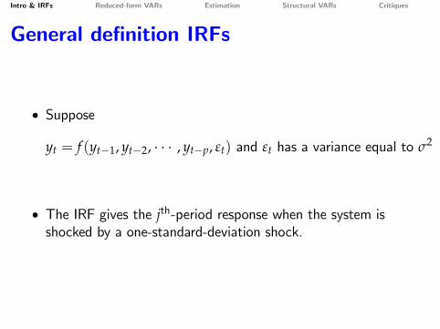
General definition IRFs
• Suppose
yt = f (yt−1, yt−2, · · · , yt−p, εt) and εt has a variance equal to σ2
• The IRF gives the jth-period response when the system isshocked by a one-standard-deviation shock.
Intro & IRFs Reduced-form VARs Estimation Structural VARs Critiques
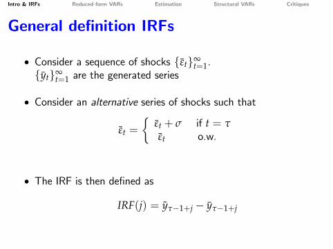
General definition IRFs
• Consider a sequence of shocks {εt}∞t=1.
{yt}∞t=1 are the generated series
• Consider an alternative series of shocks such that
εt =
{εt + σ if t = τεt o.w.
• The IRF is then defined as
IRF(j) = yτ−1+j − yτ−1+j

Intro & IRFs Reduced-form VARs Estimation Structural VARs Critiques
IRFs for linear processes
• Linear processes: The IRF is independent of the particulardraws for εt
• Thus we can simply start at the steady state (that is when εthas been zero for a very long time)
• The effect of a shock of size Λσ is Λ times the effect of ashock of size σ
Intro & IRFs Reduced-form VARs Estimation Structural VARs Critiques
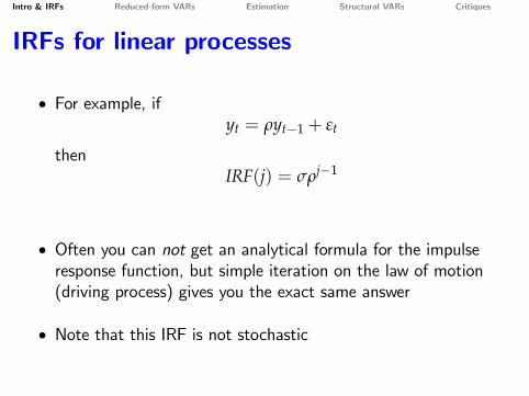
IRFs for linear processes
• For example, ifyt = ρyt−1 + εt
thenIRF(j) = σρj−1
• Often you can not get an analytical formula for the impulseresponse function, but simple iteration on the law of motion(driving process) gives you the exact same answer
• Note that this IRF is not stochastic
Intro & IRFs Reduced-form VARs Estimation Structural VARs Critiques
IRFs for nonlinear processes
• IRF depends on1 state in the period when shock occur (yt−1, yt−2, · · · yt−p)2 subsequent shocks
• Moreover, the effect of a shock of size Λσ is not Λ times theeffect of a shock of size σ
Intro & IRFs Reduced-form VARs Estimation Structural VARs Critiques
IRFs in theoretical models
• When you have solved for the policy functions, then it is trivialto get the IRFs by simply giving the system a one standarddeviation shock and iterating on the policy functions.
• Shocks in the model are structural shocks, such as• productivity shock• preference shock• monetary policy shock

Intro & IRFs Reduced-form VARs Estimation Structural VARs Critiques
IRFs in the data
The big question
• Can we estimate IRFs from the data without specifying anexplicit theoretical model
• That is what structural VARs attempt to do
Intro & IRFs Reduced-form VARs Estimation Structural VARs Critiques
VARs & IRFs
What we are going to do?
• Describe an empirical model that has turned out to be veryuseful (for example for forecasting)
• Reduced-form VAR
• Describe a way to back out structural shocks (this is the hardpart)
• Structural-VAR
Intro & IRFs Reduced-form VARs Estimation Structural VARs Critiques
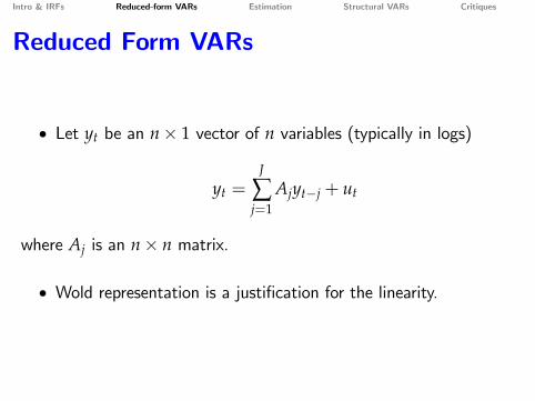
Reduced Form VARs
• Let yt be an n× 1 vector of n variables (typically in logs)
yt =J
∑j=1
Ajyt−j + ut
where Aj is an n× n matrix.
• Wold representation is a justification for the linearity.
Intro & IRFs Reduced-form VARs Estimation Structural VARs Critiques
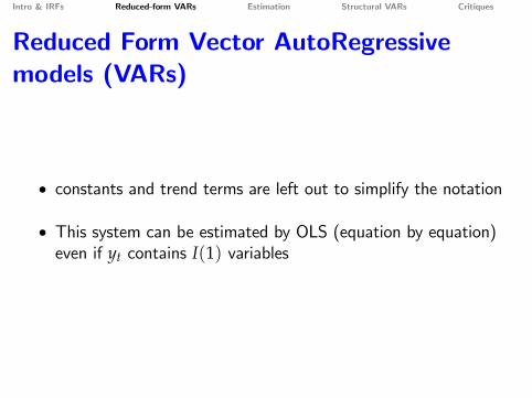
Reduced Form Vector AutoRegressivemodels (VARs)
• constants and trend terms are left out to simplify the notation
• This system can be estimated by OLS (equation by equation)even if yt contains I(1) variables
Intro & IRFs Reduced-form VARs Estimation Structural VARs Critiques
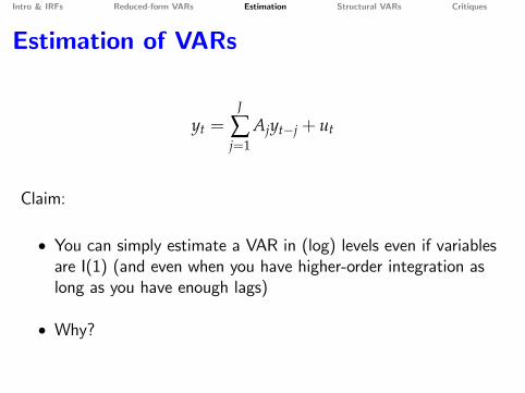
Estimation of VARs
yt =J
∑j=1
Ajyt−j + ut
Claim:
• You can simply estimate a VAR in (log) levels even if variablesare I(1) (and even when you have higher-order integration aslong as you have enough lags)
• Why?
Intro & IRFs Reduced-form VARs Estimation Structural VARs Critiques
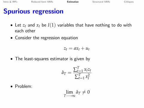
Spurious regression
• Let zt and xt be I(1) variables that have nothing to do witheach other
• Consider the regression equation
zt = axt + ut
• The least-squares estimator is given by
aT =∑T
t=1 xtzt
∑Tt=1 x2
t
• Problem:lim
T−→∞aT 6= 0

Intro & IRFs Reduced-form VARs Estimation Structural VARs Critiques
Source of spurious regressions
• The problem is not that zt and xt are I(1)• The problem is that there is not a single value for a such that
ut is stationary• If zt and xt are cointegrated then there is a value of a such that
zt − axt is stationary
• Then least-squares estimates of a are consistent• but you have to change formula for standard errors
Intro & IRFs Reduced-form VARs Estimation Structural VARs Critiques
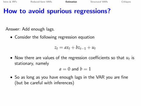
How to avoid spurious regressions?
Answer: Add enough lags.
• Consider the following regression equation
zt = axt + bzt−1 + ut
• Now there are values of the regression coeffi cients so that ut isstationary, namely
a = 0 and b = 1
• So as long as you have enough lags in the VAR you are fine(but be careful with inferences)

Intro & IRFs Reduced-form VARs Estimation Structural VARs Critiques
How to get standard errors?
• If all data series are stationary you can get standard errors usingthe usual formulas (see Hamilton 1994).
• If they are not you can use bootstrapping

Intro & IRFs Reduced-form VARs Estimation Structural VARs Critiques
Bootstrapping
• Supposeyt = ayt−1 + εt
aT =∑ ytyt−1
∑ yt−1yt−1
• How to get standard errors for IRF?technique easily generates for more complex VAR and otherstatistics

Intro & IRFs Reduced-form VARs Estimation Structural VARs Critiques
Bootstrapping
1. Estimate model and IRF
2. Calculate residuals, {εt}Tt=2 = Θ
3. Generate J new sample of length T from
zt = aTzt−1 + et
z1 = y1
et is drawn from Θ
Intro & IRFs Reduced-form VARs Estimation Structural VARs Critiques
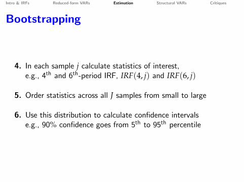
Bootstrapping
4. In each sample j calculate statistics of interest,e.g., 4th and 6th-period IRF, IRF(4, j) and IRF(6, j)
5. Order statistics across all J samples from small to large
6. Use this distribution to calculate confidence intervalse.g., 90% confidence goes from 5th to 95th percentile
Intro & IRFs Reduced-form VARs Estimation Structural VARs Critiques
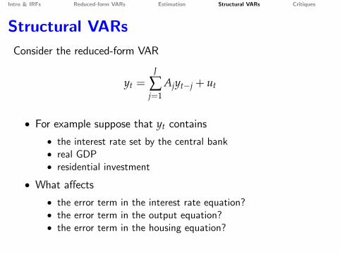
Structural VARsConsider the reduced-form VAR
yt =J
∑j=1
Ajyt−j + ut
• For example suppose that yt contains
• the interest rate set by the central bank• real GDP• residential investment
• What affects• the error term in the interest rate equation?• the error term in the output equation?• the error term in the housing equation?
Intro & IRFs Reduced-form VARs Estimation Structural VARs Critiques
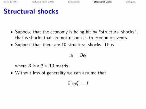
Structural shocks
• Suppose that the economy is being hit by "structural shocks",that is shocks that are not responses to economic events
• Suppose that there are 10 structural shocks. Thus
ut = Bet
where B is a 3× 10 matrix.• Without loss of generality we can assume that
E[ete′t] = I

Intro & IRFs Reduced-form VARs Estimation Structural VARs Critiques
Structural shocks
• Can we identify B from the data?
E[utu′t] = BE[ete′t]B′ = BB′
• We can get an estimate for E[utu′t] using
Σ =T
∑t=J+1
utu′t/(T− J)
• But B contains 30 unknowns and
E[utu′t
]= BB′
has only 9 equations
Intro & IRFs Reduced-form VARs Estimation Structural VARs Critiques
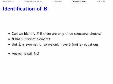
Identification of B
• Can we identify B if there are only three structural shocks?• B has 9 distinct elements• But Σ is symmetric, so we only have 6 (not 9) equations
• Answer is still NO

Intro & IRFs Reduced-form VARs Estimation Structural VARs Critiques
Identification of B
• Reason for lack of identification:Not all equations are independent. Σ1,2 = Σ2,1. For example
Σ1,2 = b11b21 + b12b22 + b13b23
but alsoΣ2,1 = b21b11 + b22b12 + b23b13
• In other words, different B matrices lead to the same Σ matrix
Intro & IRFs Reduced-form VARs Estimation Structural VARs Critiques
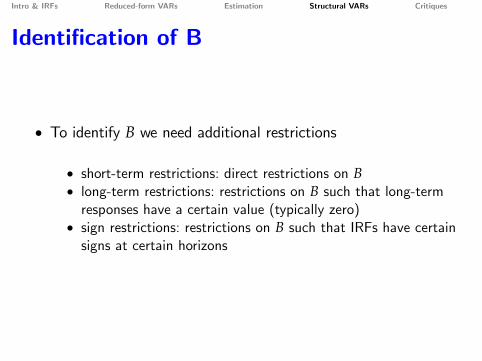
Identification of B
• To identify B we need additional restrictions
• short-term restrictions: direct restrictions on B• long-term restrictions: restrictions on B such that long-termresponses have a certain value (typically zero)
• sign restrictions: restrictions on B such that IRFs have certainsigns at certain horizons

Intro & IRFs Reduced-form VARs Estimation Structural VARs Critiques
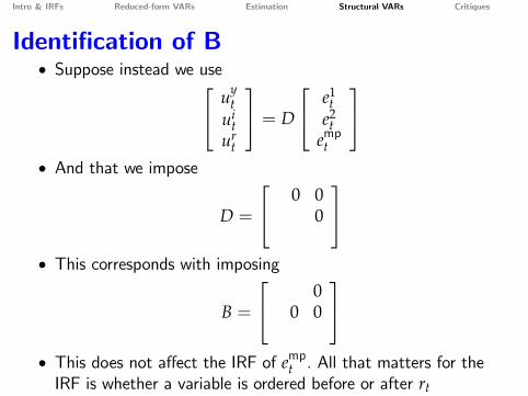
Identification of B
uit
uyt
urt
= B
e1t
e2t
empt
• Suppose we impose
B =
0 00
• Then I can solve for the remaining elements of B from
BB′ = Σ
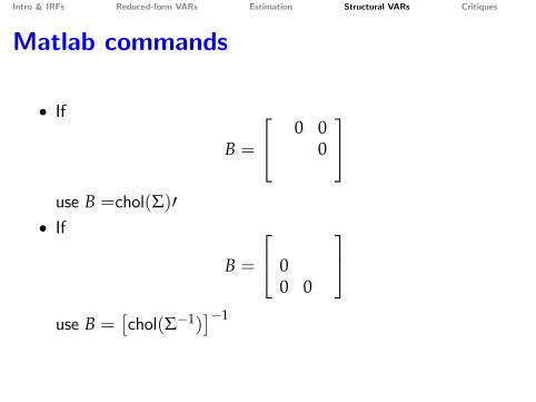
Intro & IRFs Reduced-form VARs Estimation Structural VARs Critiques
Matlab commands
• If
B =
0 00
use B =chol(Σ)′
• If
B =
00 0
use B =
[chol(Σ−1)
]−1
Intro & IRFs Reduced-form VARs Estimation Structural VARs Critiques
Identification of B• Suppose instead we use uy
tui
tur
t
= D
e1t
e2t
empt
• And that we impose
D =
0 00
• This corresponds with imposing
B =
00 0
• This does not affect the IRF of empt . All that matters for theIRF is whether a variable is ordered before or after rt
Intro & IRFs Reduced-form VARs Estimation Structural VARs Critiques
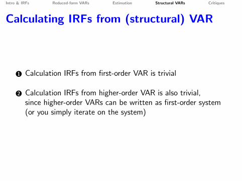
Calculating IRFs from (structural) VAR
1 Calculation IRFs from first-order VAR is trivial
2 Calculation IRFs from higher-order VAR is also trivial,since higher-order VARs can be written as first-order system(or you simply iterate on the system)
Intro & IRFs Reduced-form VARs Estimation Structural VARs Critiques
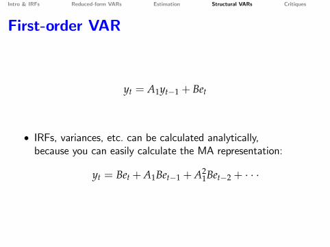
First-order VAR
yt = A1yt−1 + Bet
• IRFs, variances, etc. can be calculated analytically,because you can easily calculate the MA representation:
yt = Bet +A1Bet−1 +A21Bet−2 + · · ·

Intro & IRFs Reduced-form VARs Estimation Structural VARs Critiques
State-space notation
Every VAR can be presented as a first-order VAR. For example let
[y1,ty2,t
]= A1
[y1,t−1y2,t−1
]+A2
[y1,t−2y2,t−2
]+ B
[e1,te2,t
]
y1,ty2,t
y1,t−1y2,t−1
= [ A1 A2I2×2 02×2
] y1,t−1y2,t−1y1,t−2y2,t−2
+ [ B 02×202×2 02×2
] e1,te2,t00
Intro & IRFs Reduced-form VARs Estimation Structural VARs Critiques
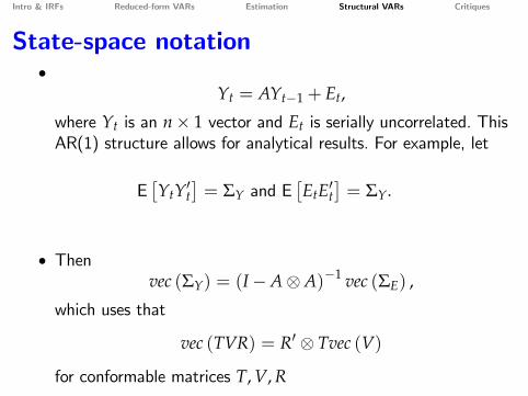
State-space notation•
Yt = AYt−1 + Et,
where Yt is an n× 1 vector and Et is serially uncorrelated. ThisAR(1) structure allows for analytical results. For example, let
E[YtY′t
]= ΣY and E
[EtE′t
]= ΣY.
• Thenvec (ΣY) = (I−A⊗A)−1 vec (ΣE) ,
which uses that
vec (TVR) = R′ ⊗ Tvec (V)
for conformable matrices T, V, R

Intro & IRFs Reduced-form VARs Estimation Structural VARs Critiques
Alternative identification assumptions
• restrictions do not have to be zero restrictions
• you can impose restrictions on B such that IRFs have certainpropertiesthen restrictions imposed depend on rest of the VAR
Intro & IRFs Reduced-form VARs Estimation Structural VARs Critiques
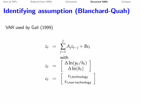
Identifying assumption (Blanchard-Quah)
VAR used by Gali (1999)
zt =J
∑j=1
Ajzt−j + Bεt
with
zt =
[∆ ln(yt/ht)
∆ ln(ht)
]εt =
[εt,technology
εt,non-technology
]

Intro & IRFs Reduced-form VARs Estimation Structural VARs Critiques
Identifying assumption (Blanchard-Quah)
• Non-technology shock does not have a long-run impact onproductivity
• Long-run impact is zero if• Response of the level goes to zero• Responses of the differences sum to zero
Intro & IRFs Reduced-form VARs Estimation Structural VARs Critiques
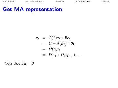
Get MA representation
zt = A(L)zt + Bεt
= (I−A(L))−1Bεt
= D(L)εt
= D0εt +D1εt−1 + · · ·
Note that D0 = B

Intro & IRFs Reduced-form VARs Estimation Structural VARs Critiques
Sum of responses
∞
∑j=0
Dj = D(1) = (I−A(1))−1B
Blanchard-Quah assumption:
∞
∑j=0
Dj =
[0]
Intro & IRFs Reduced-form VARs Estimation Structural VARs Critiques
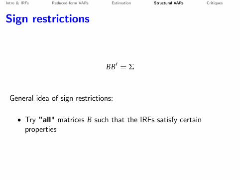
Sign restrictions
BB′ = Σ
General idea of sign restrictions:
• Try "all" matrices B such that the IRFs satisfy certainproperties
Intro & IRFs Reduced-form VARs Estimation Structural VARs Critiques
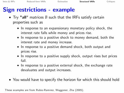
Sign restrictions - example• Try "all" matrices B such that the IRFs satisfy certainproperties such as• In response to an expansionary monetary policy shock, theinterest rate falls while money and prices rise.
• In response to a positive shock to money demand, both theinterest rate and money increase.
• In response to a positive demand shock, both output andprices rise.
• In response to a positive supply shock, output rises but pricesfall.
• In response to a positive external shock, the exchange ratedevaluates and output increases.
• You would have to specify the horizon for which this should hold
These examples are from Rubio-Ramirez, Waggoner, Zha (2005).
Intro & IRFs Reduced-form VARs Estimation Structural VARs Critiques
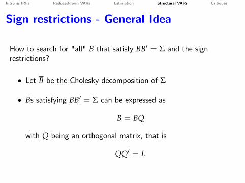
Sign restrictions - General Idea
How to search for "all" B that satisfy BB′ = Σ and the signrestrictions?
• Let B be the Cholesky decomposition of Σ
• Bs satisfying BB′ = Σ can be expressed as
B = BQ
with Q being an orthogonal matrix, that is
QQ′ = I.

Intro & IRFs Reduced-form VARs Estimation Structural VARs Critiques
Sign restrictions - In practice
"Systematically" look for Q such that
1
QQ′ = I.
2
B = QB satisfies the sign restricions

Intro & IRFs Reduced-form VARs Estimation Structural VARs Critiques
Givens matrices - Example
Q =
[Q11 Q12Q21 Q22
]
• Note thatn
∑j=1
Q2ij = 1 ∀i
=⇒∣∣Qij∣∣ ≤ 1

Intro & IRFs Reduced-form VARs Estimation Structural VARs Critiques
Sign restrictions - Givens matrices
• Suppose that B is a 2× 2 Matrix
• Then all Qs satisfying QQ′ = I can be represented with thefollowing Givens matrices
rotation : Qrot =
[cos θ − sin θsin θ cos θ
],−π ≤ θ ≤ π
reflection : Qref =
[− cos θ sin θ
sin θ cos θ
],−π ≤ θ ≤ π
• In practice you can use a grid for θ or draw θ from a uniformdistribution
Intro & IRFs Reduced-form VARs Estimation Structural VARs Critiques
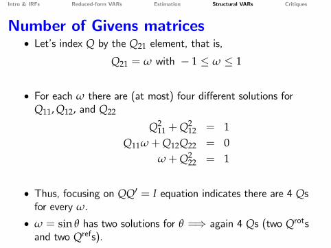
Number of Givens matrices• Let’s index Q by the Q21 element, that is,
Q21 = ω with − 1 ≤ ω ≤ 1
• For each ω there are (at most) four different solutions forQ11, Q12, and Q22
Q211 +Q2
12 = 1Q11ω+Q12Q22 = 0
ω+Q222 = 1
• Thus, focusing on QQ′ = I equation indicates there are 4 Qsfor every ω.
• ω = sin θ has two solutions for θ =⇒ again 4 Qs (two Qrotsand two Qrefs).

Intro & IRFs Reduced-form VARs Estimation Structural VARs Critiques
Givens matrices - Third Order
Qrot1 = cos θ1 − sin θ1 0
sin θ1 cos θ1 00 0 1
Qrot
2 = cos θ2 0 − sin θ20 1 0
sin θ2 0 cos θ2
Qrot
3 1 0 00 cos θ3 − sin θ30 sin θ3 cos θ3

Intro & IRFs Reduced-form VARs Estimation Structural VARs Critiques
Givens matrices - Third Order
Qref1 = − cos θ1 sin θ1 0
sin θ1 cos θ1 00 0 1
Qref
2 = − cos θ2 0 sin θ20 1 0
sin θ2 0 cos θ2
Qref
3 = 1 0 00 − cos θ3 sin θ30 sin θ3 cos θ3
Intro & IRFs Reduced-form VARs Estimation Structural VARs Critiques
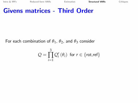
Givens matrices - Third Order
For each combination of θ1, θ2, and θ3 consider
Q =3
∏i=1
Qri (θi) for r ∈ {rot,ref}

Intro & IRFs Reduced-form VARs Estimation Structural VARs Critiques
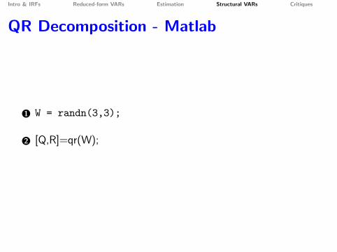
QR Decomposition
Rubio-Ramirez, Waggoner, and Zha (2005) propose the followingalternative to find orthogonal n× n matrices, which iscomputationally more effi cient for large VARs:
1 Let W be an n× n matrix, each element is an i.i.d. draw froma N (0, 1)
2 Decompose W using the QR decomposition (Householdertransformation)
W = QR,
where Q is the orthogonal matrix we are looking for
Intro & IRFs Reduced-form VARs Estimation Structural VARs Critiques
QR Decomposition - Matlab
1 W = randn(3,3);
2 [Q,R]=qr(W);

Intro & IRFs Reduced-form VARs Estimation Structural VARs Critiques
QR Decomposition - example
1
W =
−0.0551 0.1992 0.8829−1.0717 −0.4964 0.7643−0.3729 −1.6501 0.2373
2
Q =
−0.0485 0.174 0.174−0.9433 0.3156 −0.1027−0.3283 −0.9327 0.1496
Intro & IRFs Reduced-form VARs Estimation Structural VARs Critiques
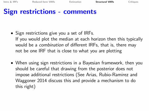
Sign restrictions - comments
• Sign restrictions give you a set of IRFs.If you would plot the median at each horizon then this typicallywould be a combination of different IRFs, that is, there maynot be one IRF that is close to what you are plotting
• When using sign restrictions in a Bayesian framework, then youshould be careful that drawing from the posterior does notimpose additional restrictions (See Arias, Rubio-Ramirez andWaggoner 2014 discuss this and provide a mechanism to dothis right)

Intro & IRFs Reduced-form VARs Estimation Structural VARs Critiques
If you ever feel bad about getting too muchcriticism ....
•
• be glad you are not a structural VAR

Intro & IRFs Reduced-form VARs Estimation Structural VARs Critiques
If you ever feel bad about getting too muchcriticism ....
•• be glad you are not a structural VAR

Intro & IRFs Reduced-form VARs Estimation Structural VARs Critiques
Structural VARs & critiques
• From MA to AR• Lippi & Reichlin (1994)
• From prediction errors to structural shocks• Fernández-Villaverde, Rubio-Ramirez, Sargent, Watson (2007)
• Problems in finite samples• Chari, Kehoe, McGratten (2008)
Intro & IRFs Reduced-form VARs Estimation Structural VARs Critiques
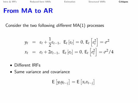
From MA to AR
Consider the two following different MA(1) processes
yt = εt +12
εt−1, Et [εt] = 0, Et
[ε2
t
]= σ2
xt = et + 2et−1, Et [et] = 0, Et
[e2
t
]= σ2/4
• Different IRFs• Same variance and covariance
E[ytyt−j
]= E
[xtxt−j
]
Intro & IRFs Reduced-form VARs Estimation Structural VARs Critiques
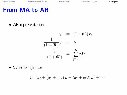
From MA to AR
• AR representation:
yt = (1+ θL) εt1
(1+ θL)yt = εt
1(1+ θL)
=∞
∑j=0
ajLj
• Solve for ajs from
1 = a0 + (a1 + a0θ) L+ (a2 + a1θ) L2 + · · ·

Intro & IRFs Reduced-form VARs Estimation Structural VARs Critiques
From MA to AR
Solution:
a0 = 1a1 = −a0θ
a2 = −a1θ = a0θ2
· · ·
You need|θ| < 1

Intro & IRFs Reduced-form VARs Estimation Structural VARs Critiques
Prediction errors and structural shocks
Solution to economic model
xt+1 = Axt + Bεt+1
yt+1 = Cxt +Dεt+1
• xt: state variables• yt: observables (used in VAR)• εt: structural shocks

Intro & IRFs Reduced-form VARs Estimation Structural VARs Critiques
Prediction errors and structural shocks
• From the VAR you get prediction error et+1
et+1 = yt+1 − Et [yt+1]
= Cxt +Dεt+1 − Et [Cxt]
= C (xt − Et [xt]) +Dεt+1
• Problem: Not guaranteed that
xt = Et [xt]

Intro & IRFs Reduced-form VARs Estimation Structural VARs Critiques
Prediction errors and structural shocks
• Suppose: yt = xt
• that is, all state variables are observed
• Thenxt = Et [xt]

Intro & IRFs Reduced-form VARs Estimation Structural VARs Critiques
Prediction errors and structural shocks
• Suppose: yt 6= xt
• Has yt has enough info to uncover xt and, thus, εt?

Intro & IRFs Reduced-form VARs Estimation Structural VARs Critiques
Prediction errors and structural shocks• Suppose D is invertible
εt = D−1 (yt+1 − Cxt)
=⇒xt+1 = Axt + BD−1 (yt+1 − Cxt)
=⇒
xt+1
(I−
(A+ BD−1C
)L)= yt+1
• =⇒
xt = Et [xt] if
the eigenvalues of A− BD−1Cmust be strictly less than 1 in modulus
• See F-V,R-R,S, W (2007)
Intro & IRFs Reduced-form VARs Estimation Structural VARs Critiques
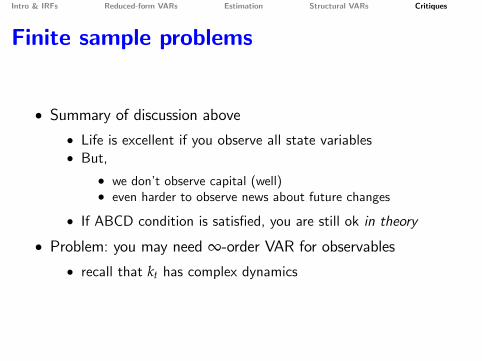
Finite sample problems
• Summary of discussion above• Life is excellent if you observe all state variables• But,
• we don’t observe capital (well)• even harder to observe news about future changes
• If ABCD condition is satisfied, you are still ok in theory
• Problem: you may need ∞-order VAR for observables• recall that kt has complex dynamics
Intro & IRFs Reduced-form VARs Estimation Structural VARs Critiques
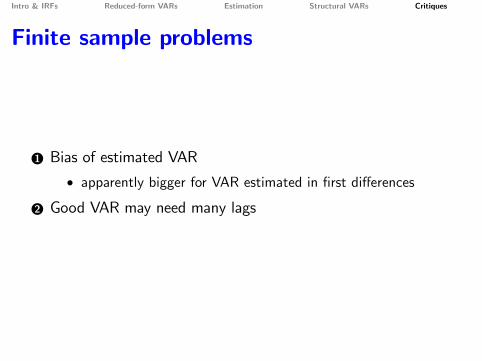
Finite sample problems
1 Bias of estimated VAR
• apparently bigger for VAR estimated in first differences
2 Good VAR may need many lags
Intro & IRFs Reduced-form VARs Estimation Structural VARs Critiques
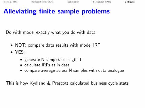
Alleviating finite sample problems
Do with model exactly what you do with data:
• NOT: compare data results with model IRF• YES:
• generate N samples of length T• calculate IRFs as in data• compare average across N samples with data analogue
This is how Kydland & Prescott calculated business cycle stats
Intro & IRFs Reduced-form VARs Estimation Structural VARs Critiques
References• Arias, J.E., J.F. Rubio-Ramirez, D.F. Waggoner, Inference Based on SVARs Identified
with Sign and Zero Restrictions: Theory and Applications, Federal Reserve Board
International Finance Discussion Paper 2014-1100. Available at
• http://www.federalreserve.gov/pubs/ifdp/2014/1100/default.htm.
• Chari, V.V., P.J. Kehoe, E.R. McGrattan, 2008, Are structural VARs with long-run
restrictions useful in developing business cycle theory?, Journal of Monetary Economics,
55, 1337-52.
• Fernandez-Villaverde, J., J.F. Rubio-Ramirez, T.J. Sargent, and M.Watson, 2007, ABCs
(and Ds) of Understanding VARs, Econometrica, 97, 1021-26.
Gives conditions whether a particular VAR can infer structural shocks.
• Fry, R. and A. Pagan, 2011, Sign Restrictions in Structual Vector Autoregressions: A
Critical Review, Journal of Economic Literature, 49, 938-960.
• overview of sign restrictions in VARs and detailed discussion of its weaknesses

Intro & IRFs Reduced-form VARs Estimation Structural VARs Critiques
• Kilian, Lutz, 2011, Structural Vector Autogressions.
• Overview paper that gives several examples of identification choices for different
theoretical models. Available at
• http://www-personal.umich.edu/~lkilian/elgarhdbk_kilian.pdf.
• Lippi, M., and L. Reichlin, 1994, VAR analysis, nonfundamental representations,
Blaschke matrices, Journal of Econometrics, 63, 307-325.
• Luetkepohl, H., 2011, Vector Autoregressive Models, EUI Working Papers
ECO2011/30.
• detailed paper on estimating and working with VARs. Available at
• cadmus.eui.eu/bitstream/handle/1814/19354/ECO_2011_30.pdf

Intro & IRFs Reduced-form VARs Estimation Structural VARs Critiques
• Rubio-Ramirez, Juan F., D.F. Waggoner, and T. Zha, 2005, Markov-Switching
Structural Vector Autogressions: Theory and Applications, Federal Reserve Bank of
Atlanta Working Paper 2005-27.
• contains a detailed discussion of different identification schemes and sign
restrictions in particular. Available at
• http://www.frbatlanta.org/filelegacydocs/wp0527.pdf.
• Whelan, K.,2014 MA Advanced Macroeconomics.
• Set of slides with more detailed info and a discussion of several empirical
examples. Available at
• http://www.karlwhelan.com/MAMacro/part2.pdf
• http://www.karlwhelan.com/MAMacro/part3.pdf
• http://www.karlwhelan.com/MAMacro/part4.pdf


