1 VECTOR-BASED GROUND SURFACE AND OBJECT REPRESENTATION USING CAMERAS By JAESANG LEE A DISSERTATION PRESENTED TO THE GRADUATE SCHOOL OF THE UNIVERSITY OF FLORIDA IN PARTIAL FULFILLMENT OF THE REQUIREMENTS FOR THE DEGREE OF DOCTOR OF PHILOSOPHY UNIVERSITY OF FLORIDA 2009
Transcript
1
VECTOR-BASED GROUND SURFACE AND OBJECT REPRESENTATION USING CAMERAS
By
JAESANG LEE
A DISSERTATION PRESENTED TO THE GRADUATE SCHOOL OF THE UNIVERSITY OF FLORIDA IN PARTIAL FULFILLMENT
OF THE REQUIREMENTS FOR THE DEGREE OF DOCTOR OF PHILOSOPHY
UNIVERSITY OF FLORIDA
2009
Report Documentation Page Form ApprovedOMB No. 0704-0188
Public reporting burden for the collection of information is estimated to average 1 hour per response, including the time for reviewing instructions, searching existing data sources, gathering andmaintaining the data needed, and completing and reviewing the collection of information. Send comments regarding this burden estimate or any other aspect of this collection of information,including suggestions for reducing this burden, to Washington Headquarters Services, Directorate for Information Operations and Reports, 1215 Jefferson Davis Highway, Suite 1204, ArlingtonVA 22202-4302. Respondents should be aware that notwithstanding any other provision of law, no person shall be subject to a penalty for failing to comply with a collection of information if itdoes not display a currently valid OMB control number.
1. REPORT DATE DEC 2009 2. REPORT TYPE
3. DATES COVERED 00-00-2009 to 00-00-2009
4. TITLE AND SUBTITLE Vector-Based Ground Surface and Object Representation Using Cameras
5a. CONTRACT NUMBER
5b. GRANT NUMBER
5c. PROGRAM ELEMENT NUMBER
6. AUTHOR(S) 5d. PROJECT NUMBER
5e. TASK NUMBER
5f. WORK UNIT NUMBER
7. PERFORMING ORGANIZATION NAME(S) AND ADDRESS(ES) University of Florida,Center for Intelligent Machines and Robotics (CIMAR),Gainesville,FL,32611
8. PERFORMING ORGANIZATIONREPORT NUMBER
9. SPONSORING/MONITORING AGENCY NAME(S) AND ADDRESS(ES) 10. SPONSOR/MONITOR’S ACRONYM(S)
11. SPONSOR/MONITOR’S REPORT NUMBER(S)
12. DISTRIBUTION/AVAILABILITY STATEMENT Approved for public release; distribution unlimited
13. SUPPLEMENTARY NOTES
14. ABSTRACT Computer vision plays an important role in many fields these days. From robotics to biomedical equipmentto the car industry to the semi-conductor industry, many applications have been developed for solvingproblems using visual information. One computer vision application in robotics is a camera-based sensormounted on a mobile robot vehicle. Since the late 1960s this system has been utilized in various fields, suchas automated warehouses, unmanned ground vehicles, space robots, and driver assistance systems. Eachsystem has a different mission, like terrain analysis and evaluation, visual odometers, lane departurewarning systems, and identification of such moving object as other cars and pedestrians. Thus, variousfeatures and methods have been applied and tested to solve different computer vision tasks. A main goal ofthis vision sensor for an autonomous ground vehicle is to provide such continuous and precise perceptioninformation as traversable paths, future trajectory estimations and lateral position error corrections withsmall data size. To accomplish these objectives, multicamera- based Path Finder and Lane Finder SmartSensors were developed and utilized on an autonomous vehicle at the University of Florida?s Center forIntelligent Machines and Robotics (CIMAR). These systems create traversable area information for bothan unstructured road environment and an urban environment in real time. Extracted traversableinformation is provided to the robot?s intelligent system and control system in vector data form throughthe Joint Architecture for Unmanned Systems (JAUS) protocol. Moreover, a small data size is used torepresent the real world and its properties. Since vector data are small enough for storing, retrieving, andcommunication, traversability data and its properties are stored at the World Model Vector KnowledgeStore for future reference.
15. SUBJECT TERMS
16. SECURITY CLASSIFICATION OF: 17. LIMITATION OF ABSTRACT Same as
Report (SAR)
18. NUMBEROF PAGES
153
19a. NAME OFRESPONSIBLE PERSON
a. REPORT unclassified
b. ABSTRACT unclassified
c. THIS PAGE unclassified
Standard Form 298 (Rev. 8-98) Prescribed by ANSI Std Z39-18
Motivation ...............................................................................................................................15 Literature Review ...................................................................................................................15
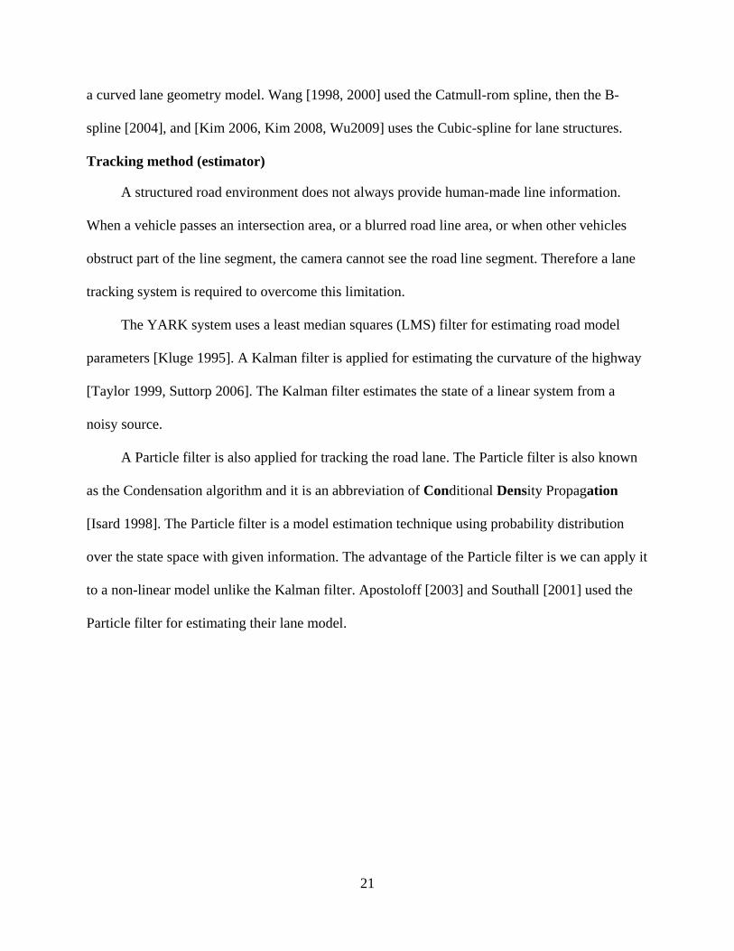
Lane Tracking ..................................................................................................................19 Feature selection .......................................................................................................19 Lane extraction .........................................................................................................19 Lane model ...............................................................................................................20 Tracking method (estimator) ....................................................................................21
2 RESEARCH GOAL ...............................................................................................................22
Problem Statement ..................................................................................................................22 Development ...........................................................................................................................22 Further Assumptions ...............................................................................................................23
3 PATH FINDER SMART SENSOR .......................................................................................24
Introduction .............................................................................................................................24 Feature Space ..........................................................................................................................24
RGB Color Space ............................................................................................................25 Normalized RGB Color Space ........................................................................................25
Training Area ..........................................................................................................................26 Classifier .................................................................................................................................27
Maximum Likelihood ......................................................................................................27
6
Mixture of Gaussians .......................................................................................................28 Expectation and Maximization (EM) Algorithm ............................................................30
4 LANE FINDER SMART SENSOR .......................................................................................53
Introduction .............................................................................................................................53 Camera Field of View .............................................................................................................54 Canny Edge Detector ..............................................................................................................54 First Order Line Decision .......................................................................................................55
Hough Transform ............................................................................................................56 Lane Line Search .............................................................................................................58
Polynomial Line Decision ......................................................................................................58 Cubic Splines ...................................................................................................................59 Control Points ..................................................................................................................61
Lane Model .............................................................................................................................62 Lane Estimation ......................................................................................................................63 Lane Center Correction ...........................................................................................................65
Lane Correction by Two Cameras ...................................................................................65 Lane Correction by One Camera .....................................................................................68
Lane Property ..........................................................................................................................68 Uncertainty Management ........................................................................................................70
5 VECTOR-BASED GROUND AND OBJECT REPRESENTATION ...................................97
Introduction .............................................................................................................................97 Approach .................................................................................................................................97 Ground Surface Representation ..............................................................................................99 Static Object Representation .................................................................................................100 World Model Vector Knowledge Store ................................................................................101
6 EXPERIMENTAL RESULTS AND CONCLUSIONS .......................................................111
LFSSWing test results ...................................................................................................115 The PFSS test result .......................................................................................................117 Building vector-based map ............................................................................................118
Conclusions ...........................................................................................................................118 Future Work ..........................................................................................................................119
7
LIST OF REFERENCES .............................................................................................................148
3-8 Classifier error for Citra and DARPA Grand Challenge 2005 scene with varying numbers of mixture-of-Gaussian distributions.. ................................................................46
3-9 Two Gaussian distribution’ absolute mean values over the iteration step for the DARPA Grand Challenge 2005 image. .............................................................................47
3-10 Classification result ............................................................................................................48
5-7 Lane objects and stored polygon points (red points). ......................................................110
6-1 CIMAR Navigator III, Urban NaviGator.. .......................................................................123
6-2 NaviGator III camera sensor systems.. ............................................................................124
6-3 The PFSS software. ..........................................................................................................128
6-4 The LFSSWing software..................................................................................................131
11
6-5 The LFSS Arbiter and the RN screen. .............................................................................132
6-6 Urban NaviGator 2009 system architecture. ....................................................................133
6-7 The LFSSWing test result at the Gainesville Raceway. ..................................................136
6-8 The LFSSWing test results at the University of Florida campus.....................................139
6-9 The LFSSWing test results in the urban road. .................................................................140
6-10 The LFSSWing test results at the University of Florida with nighttime setting. .............141
6-11 The PFSS test results in the Gainesville Raceway. Source, segmented and the TIN control points’ images, respectively. ...............................................................................144
6-12 The PFSS test results in the University of Florida campus. Source, segmented and the TIN control points’ images, respectively. ..................................................................145
6-13 The LFSSWing vector-based representation. ..................................................................146
6-14 The PFSS vector-based representation ............................................................................147
12
LIST OF ABBREVIATIONS
DARPA Defense Advanced Research Projects Agency
DGC 2005 DARPA Grand Challenge 2005
DUC 2007 DARPA Urban Challenge 2007
GPS Global Positioning System
IMU Inertial Measurement Unit
INS Inertial Navigation System
JAUS Joint Architecture for Unmanned Systems
LADAR Light Detection and Ranging
LFSS Lane Finder Smart Sensor component software
LFSSWing Lane Finder Smart Sensor Wing component software
LFSS Arbiter Lane Finder Arbiter Smart Sensor component software
NFM North Finding Module
PFSS (Vision-based) Path Finder Smart Sensor component software
WMVKS World Model Vector Knowledge Store Smart Sensor component software
13
Abstract of Dissertation Presented to the Graduate School of the University of Florida in Partial Fulfillment of the Requirements for the Degree of Doctor of Philosophy
VECTOR-BASED GROUND SURFACE AND OBJECT REPRESENTATION
USING CAMERAS
By
Jaesang Lee
December 2009 Chair: Carl D. Crane III Major: Mechanical Engineering
Computer vision plays an important role in many fields these days. From robotics to bio-
medical equipment to the car industry to the semi-conductor industry, many applications have
been developed for solving problems using visual information. One computer vision application
in robotics is a camera-based sensor mounted on a mobile robot vehicle. Since the late 1960s,
this system has been utilized in various fields, such as automated warehouses, unmanned ground
vehicles, space robots, and driver assistance systems. Each system has a different mission, like
terrain analysis and evaluation, visual odometers, lane departure warning systems, and
identification of such moving object as other cars and pedestrians. Thus, various features and
methods have been applied and tested to solve different computer vision tasks.
A main goal of this vision sensor for an autonomous ground vehicle is to provide such
continuous and precise perception information as traversable paths, future trajectory estimations,
and lateral position error corrections with small data size. To accomplish these objectives, multi-
camera-based Path Finder and Lane Finder Smart Sensors were developed and utilized on an
autonomous vehicle at the University of Florida’s Center for Intelligent Machines and Robotics
14
(CIMAR). These systems create traversable area information for both an unstructured road
environment and an urban environment in real time.
Extracted traversable information is provided to the robot’s intelligent system and control
system in vector data form through the Joint Architecture for Unmanned Systems (JAUS)
protocol. Moreover, a small data size is used to represent the real world and its properties. Since
vector data are small enough for storing, retrieving, and communication, traversability data and
its properties are stored at the World Model Vector Knowledge Store for future reference.
15
CHAPTER 1 INTRODUCTION
Motivation
Computer vision plays an important role in many fields these days. From robotics to bio-
medical equipment to the car industry to the semi-conductor industry, many applications have
been developed for problems using visual information. Since the price of camera sensors is
falling and they are now less expensive and gather more information than light detection and
ranging (LADAR) sensors, their use for applicable problem solving seems assured.
One computer vision application in robotics is a camera-based sensor mounted on a mobile
robot vehicle. Since the late 1960s, this system has been utilized in various fields, such as
automated warehouses, unmanned ground vehicles, space robots, and driver assistance systems
[Gage 1995, McCall 2006, Matthies 2007]. Each system has a different mission. For example,
systems provide terrain analysis and evaluation, visual odometers, lane departure warning
systems, and moving object like other cars and pedestrians identification.
Thus, various features and methods have been applied and tested for solving different
computer vision tasks. A main goal of the vision sensor for autonomous ground vehicle sensor
development is to provide continuous and precise perception information, such as traversable
path, future trajectory estimation, lateral position error correction, and moving and static object
classification or identification. The prior work associated with the tasks of terrain analysis and
the identification of roadway lanes is discussed in the literature review sections.
Literature Review
This chapter describes the various methods and algorithms that were developed to
accomplish terrain analysis, lane extraction, and tracking. A terrain analysis covers feature
16
selection, classifier selection, and sensor fusion. A lane tracking covers feature selection, lane
extraction, lane model assumption, and tracking method.
Terrain Analysis
Feature selection
Terrain analysis and estimation is an essential and basic goal of autonomous vehicle
development. For off-road situations, a lack of environmental structure, plus hazardous
situations, and difficulty of prediction inhibit an accurate and constant path evaluation. The key
step of terrain estimation starts with proper feature selection, which is applied to the classifier.
In addition to Light Detection and Ranging (LADAR) distance information, the visual
information is a good source for analyzing traversable terrain. Consequently, image intensity,
various color models, texture information, and edges have been suggested and utilized for the
main input for vision-based terrain estimation.
One primary feature, an intensity image, is used for terrain estimation [Sukthankar 1993,
Pomerleau 1995]. The intensity image is easy to understand and requires only a small processing
time, but lacks information. Many edge-based path finding systems [Behringer 2004] and stereo
vision systems have used gray images to find disparities between two images [Bertozzi 1998,
Kelly 1998].
The next and most commonly used feature is the red-blue-green (RGB) color space. The
RGB color space is the standard representation in computer and digital cameras; therefore, it is
widely known and easily analyzed. The Carnegie-Mellon Navlab vehicle used a color video
camera and the RGB color space as a feature for following a road [Thorpe 1987]. Road and non-
road RGB color models are generated and applied to color classification algorithms.
17
Another color vision system is the Supervised Classification Applied to Road Following
(SCARF) system that detects unstructured roads and intersections for intelligent mobile robots
[Crisman 1993]. This system can navigate a road that has no lanes or edge lines, or has degraded
road edges and road surface scars.
The most common and challenging camera problem is that data are affected by changes in
illumination from one time to another, which results in an inconstant color source. This is the
biggest challenge to an outdoor vision-based robot system. Normalized RGB is one method used
to overcome lighting effects in the color-based face recognition system [Vezhnevets 2003] and in
many other fields [Bräunl 2008]. Normalization of the RGB color space makes the system less
sensitive to certain color channels. In terms of hardware, attaching a polarizing filter on the
camera has been considered.
Other research in vehicle sensor development introduces different color spaces, like hue
and saturation, as additional features within the RGB color space [Bergquist 1999]. The RGB
color space is also used as a primary feature for object detection and identification, as well as
terrain estimation.
Another approach to road segmentation is a texture-based system. Zhang [1994] utilized
road texture orientation using a gray image as one road segmentation feature, as well as image
coordinate information. Chandler [2003] applied texture information to an autonomous lawn
mowing machine. The discrete cosine transform (DCT) and discrete wavelet transformation were
applied to distinguishing tall grass areas and mowed grass area.
18
Classifier
An autonomous vehicle is a real-time, outdoor application, and its color camera input size
is relatively large. For these reasons, a simple and strong algorithm is demanded when selecting
a classifier.
The Bayesian algorithm used with the RGB color space is applied as a classification
algorithm in the Navlab vehicle [Thorpe 1988, Crisman 1993]. Road and non-road Gaussian
models were generated using color pixels and applied to whole image pixels for road
classification.
Davis [1995] implemented two different algorithms: the Fisher Linear Discriminant (FLD)
applied to two-dimensional RG color feature space and the Backpropagation Neural Network
was applied to a three-dimensional RGB color feature space.
Monocular vision, stereo vision, LADAR, or sensor fusion
Different types of perception systems have been developed using different type sensors,
such as a monocular vision camera, stereo vision camera, Light Detection and Ranging (LADAR)
sensor and camera-LADAR fusion sensor [Rasmussen 2002]. The monocular vision system is
found in the Carnegie-Mellon Navlab and SCARF system [Thorpe 1988, Davis 1995]. A camera
is mounted on the front in the middle of the car and faces the ground. The source image is
resized for computation efficiency. Sukthankar [1993] used a steerable camera to improve the
camera field of view in sharp turn situations.
Unlike the monocular vision system, a stereo vision system can detect not only terrain area,
but also obstacle distance. The Real-time Autonomous Navigator with a Geometric Engine
(RANGER) uses stereo vision for determining the traversable area of the terrain [Kelly 1997].
19
The Generic Obstacle and Lane Detection (GOLD) stereo vision system detects obstacles and
estimates obstacle distance at a rate of 10Hz [Bertozzi 1998].
Lane Tracking
Feature selection
Urban areas have artificial structures for example, road lane markings, traffic signals, and
information signals. The first step for a vision-based road-following system in an urban area is
road line marking extraction. To meet this goal, many systems use different features. For
where X is a vector of traversability grid map coordinates, x is a vector of image plane
coordinates, and H is a transformation matrix. In a 2-D plane, Eq (3-19) can be represented in
linear form by
1 11 12 13 1
2 21 22 23 2
3 31 32 33 3
X h h h xX h h h xX h h h x
=
. (3-20)
Eq (3-20) can be rewritten in inhomogeneous form,
11 12 131
3 31 32 33
,h x h y hXXX h x h y h
+ += =
+ + (3-21)
and
21 22 232
3 31 32 33
h x h y hXYX h x h y h
+ += =
+ +. (3-22)
Since there are eight independent elements in Eq (3-20), only 4 reference points are needed to
solve for the H matrix.
111 1 1 1 1 1 1
121 1 1 1 1 1 1
132 2 2 2 2 2 2
212 2 2 2 2 2 2
22
234 4 4 4 4 4 4
314 4 4 4 4 4 4
32
1 0 0 00 0 0 1
1 0 0 00 0 0 1
... ...1 0 0 0
0 0 0 1
hx y X x X y X
hx y Y x Y y Y
hx y X x X y X
hx y Y x Y y Y
hh
x y X x X y Xh
x y Y x Y y Yh
− −
− − − − =− − − − − −
(3-23)
Eq (3-23) is in A bλ= form. For solving Eq (3-23) equation, a pseudo-inverse method is applied:
1( ) .T TA A A Bλ −= (3-24)
Finally, the H transformation matrix is calculated using Eq (3-24) and it is used to convert
the segmented image to a traversability grid map image. Figure 3-14 (A, B) shows the classified
38
image, Figure 3-14 (C, D) shows the transformed image without pixel interpolation, and Figure
3-14 (E, F) shows the transformed image with pixel interpolation. In each subfigure (Figures 3-
14 C, D, E, F), the vehicle is located at the center of the image (blue square) with its direction
indicated by a thin black line.
Since a wide-angle lens is used in the camera assembly, a broad swath of the road is
captured. However, as a result of that wide angle, there is an appreciable distortion in distant
regions of the image. This distortion results in only a small amount of pixels representing most
of the distant portion of the image. This fact results in the transformation generating a mapped
image with “holes” in the distant regions of the map. These holes can then be filled by linear
interpolation with respect to the row number of each pixel (see Figure 3-14 (C, E)). After
creating a traversability grid map, the GPS and INS yaw data are applied to convert local
coordinates into global coordinates.
39
A
B C
Figure 3-1. CIMAR Navigator II Path Finder system for DARPA Grand Challenge 2005. A) camera assembly, B) computer and electronics enclosure, and C) computer housing.
40
A
B
Figure 3-2. Sample unstructured environment. A) Citra, FL., B) DARPA Grand Challenge 2005 course, NV.
41
A
B
Figure 3-3. Sample structured road environment. A) Gainesville Raceway, Gainesville, FL., B) DARPA Urban Challenge 2007 Area-C course, CA.
42
Figure 3-4. RGB (red, green, blue) color space.
43
A
B
Figure 3-5. Training area selection. A) Unstructured road, B) structured road.
44
A B
C D
E F
Figure 3-6. RGB distribution of road training area and background training area. A) Road at Citra, B) DARPA Grand Challenge 2005 course road, C) background at Citra, D) DARPA Grand Challenge 2005 course background, E) road and background at Citra, and F) DARPA Grand Challenge 2005 course road and background
45
Figure 3-7. Classified road images. A) Bayesian classification result of Citra, B) Bayesian
classification result of DARPA Grand Challenge 2005 course, C) EM classification result of Citra, and D) EM classification result of DARPA Grand Challenge 2005 course.
46
Figure 3-8. Classifier error for Citra and DARPA Grand Challenge 2005 scene with varying
numbers of mixture-of-Gaussian distributions. The X axis shows the number of Gaussian distributions for the road training region and background training region.
47
A
B
Figure 3-9. Two Gaussian distribution’ absolute mean values over the iteration step for the DARPA Grand Challenge 2005 image. A) First Gaussian mean, B) Second Gaussian mean.
48
A
B
C
D
Figure 3-10. Classification result. A) Source image, B) pixel-based classification result, C) 4x4 block-based classification result, and D) 9x9 block-based classification result.
Figure 3-12. Coordinate systems. A) Relationship between camera view and world view and B) relationship between camera coordinate system, vehicle coordinate system, and earth coordinate system.
51
A
B
Figure 3-13. Perspective transformation reference points. A) Green dots are reference points in 320 × 108 size image at Flavet Field, University of Florida, and B) Green squares are reference points in a 40 × 40 meter traversability grid map image with 1 meter resolution. Red square is a vehicle.
52
A B
C D
E F
Figure 3-14. Transformed image. A) Classified image of Citra, B) classified image of DARPA Grand Challenge 2005 course, C) traversability grid map image without interpolation of Citra, D) traversability grid map image without interpolation of DARPA Grand Challenge 2005 course, E) traversability grid map image with interpolation, and F) traversability grid map image with interpolation.
53
CHAPTER 4 LANE FINDER SMART SENSOR
Introduction
The first period of autonomous vehicle development involved operating in an off-road
environment where there were no lane demarcations, for example the DARPA Grand Challenge
2005 system and the Mars Explorer robot vehicle. However, at present, most vehicles drive in an
urban environment that is generally paved with lanes defined by painted lines. Also, many
autonomous vehicles depend on a Global Positioning System (GPS) to compute current location
and project routes to desired locations. Unfortunately, GPS provides less accurate positioning
solutions in the urban environment than in an open area environment, since urban infrastructure
can blocks satellite signals or cause multi-path signals.
An urban traffic area provides more traffic facilities than off-road or highway. These
facilities include bike lanes, curbs, sidewalks, crossroads, and various traffic signals. These
urban environment facilities help human drivers understand their surroundings. In other words,
from the point of view of robot perception, it also increases the complexity of the surroundings.
On the highway, the lane lines are usually well-marked, with no sharp curvatures and no
oncoming traffic. Therefore, with a driver assistant system, it turns out that highway driving is
simpler than inner-city driving [Bräunl 2008].
The outdoor environment also presents an array of difficulties, including dynamic lighting
conditions, poor road conditions, and road networks that are not consistent from region to region.
Because of these limitations, an autonomous vehicle that is designed for urban driving needs a
more adaptive lane tracking system. In this chapter, the lane and its property extraction and
tracking system for an autonomous vehicle in an urban environment are described.
54
Camera Field of View
Two different field of view camera systems are applied to the Lane Finder Smart Sensor.
Each vision system uses a different camera field of view and range to improve overall lane
tracking system output. Figure 4-1 is a diagram of the camera field of view diagram. Figure 4-1
(A) shows the long-range field of view camera, mounted at the center of the vehicle, and Figure
4-1 (B) shows the short-range, but wide field of view of those two cameras. Two short-range
cameras capture the source image from the vehicle front, so it provides enough high resolution
and clear road lane source to calculate not only lane tracking, but also lane properties. Also, the
two camera-based system provides a clear lane image even if another vehicle stands or travels in
front of the robot vehicle. Figure 4-2 (A) and (B) show a two camera-based sample source image.
A long-range camera is a good source for future trajectory estimation. Its resolution is less
than a close view camera, but it can see the area further down the road. Figure 4-2 (C) and (D)
shows a long-range center camera sample image.
Canny Edge Detector
A road is defined by several characteristics. These may include color, shape, texture, edges,
corners, and other features. In particular, the road lane is a human-made artificial boundary line
that is marked with color and type information. Consequently, road lane lines contain dominant
edge information and this cue is the most important feature for extracting road lane information.
The edge of an image is created by several factors, for example, different 3-D object depths on a
2-D image plane, different reflection rates on a surface, various illumination conditions, and
sudden object orientation variation.
Edge detection is accomplished by use of the Canny edge filter [Nixon 2008]. The Canny
edge filter utilizes a pre-noise removing step and then computes omni-directional edge
55
information. Finally, it uses two threshold values that requires the detector to utilize much tuning
and yields a sufficiently segmented image. Because of this multi-step approach, the Canny edge
detector is widely used in many fields.
The following four steps comprise the Canny edge filter algorithm:
• Apply a derivative of a Gaussian noise filter.
• Compute x, y gradients, which are Sobel edge detection and gradient magnitude, respectively.
• Apply non-maximum suppression.
o Thin multi-pixel wide “ridges” down to a single pixel width.
• Add linking and thresholding.
o Use low, high edge-strength thresholds,
o Accept all edges over low threshold that are connected to edges over high threshold.
To further enhance the edge detector’s performance, only the red channel of the source
image is processed. This channel is used because it has the greatest content in both yellow and
white and thus can provide the greatest contrast between yellow/white regions and asphalt
background. Figure 4-3 depicts the results of the Canny edge filter with two sets of threshold
values and Figure 4-4 shows Canny filter results in various situations.
First Order Line Decision
The lane finder software has two main functions. One is to establish lane departure
warning and tracking, and the other is future trajectory estimation. For the first goal, there is no
need for distance to detect a curved line. If the camera sees a local area, curved lines looks like
straight lines. Therefore, a first-order line solution is applied for a lane departure warning system.
It provides a lane center position with respect to the current driving vehicle position. This
56
solution is more robust and faster than a high order line solution; therefore, processing update
rates can be increased.
For trajectory estimation, the camera has to see as far as it can because farther sight
information provides greater environmental understanding for the vehicle. This information is
used by the control element and consequently the control element can manage the vehicle at
higher speed. However, if the camera has farther sight, just by the nature of the road, it can see
many curved lines. Therefore, a higher order line solution is necessary for future trajectory
estimation.
Hough Transform
The Hough transform is a technique that locates a certain shape in an image. The Hough
transform was first implemented to find lines in images [Duda 1972] and it has been extended to
further applications. It is a robust tool for extracting lines, circles, and ellipses. One advantage of
the Hough transform in the lane extracting application is that it works well with many noise
edges and/or partial line edges. From this point of view, the Hough transform can provide the
same result as the template matching technique, but it uses many fewer computational resources
[Nixon 2008]. Two disadvantages of the Hough transform is that it requires a large storage space
and high processing power, and it produces as many lines as it can detect from the source image.
Therefore, searching for road lane lines among all the detected Hough lines is necessary.
The Hough transform algorithm is as follows:
If one considers a line in an image domain, its equation can be written as
,y mx c= + (4-1)
or
57
cos sin ,x yθ θ ρ+ = (4-2)
where ρ is a distance from the image domain origin to the line and θ is the orientation of ρ
(the line from the origin perpendicular to the modeled line) with respect to the X-axis, as
illustrated in Figure 4-5. Based on Eq (4-2), one can generate a Hough parameter space that
plots possible ( ρ ,θ ) values, which are defined by (x, y) points in the image. Finally, strong lines
can be selected by searching maximum values in the Hough parameter space ( ρ ,θ ). Figure 4-6
(B) shows the Hough space diagram when using the Canny filtered edge image in Figure 4-6 (A).
The maximum ( ρ ,θ ) values in the Hough space is the strongest line in the image domain.
However, this method cannot guarantee to extract a road lane line since an edge extracted image
contains various noise pixels for many reasons. For example, an old tire track can register as a
line in the road figure 4-4 (H) and different reflections from the road can appear to be a straight
line like the edge in figure 4-4 (B).
Figure 4-7 shows the Hough transform line result in various situations. Figure 4-7 (B)
show when a vehicle passes a crossroad area, so stop lines are detected. Also, another artificial
line is easily detected and lane lines are blocked by other objects like grass. This case is shown in
figure 4-7 (C). Figure 4-7 (D), right image, shows random noise edge pixels become a line object
by coincidence. Due to the differing reflection rates of the road surface, a different reflection
boundary area can create strong edges and can cause a false line object. Figure 4-7 (E) and (F),
left images, illustrate this situation.
Because of this Hough transform property and various real world situations, two steps are
required to correct it; a few lane candidate lines are extracted from the Hough space, then lane
lines are searched for among the candidate Hough lines.
58
Lane Line Search
The Hough transform for line extraction finds many lines. These include not just road lane
lines, but also other lines, like a crosswalk lane, for example [Hashimoto 2004]. Figure 4-7
shows sample results of this process. Consequently, among the candidate Hough lines, searching
lane lines by using the properties of lane lines is a necessary step.
Since road lane lines are parallel to each other and usually at the same angle, two
parameters are used for searching the lane lines: angle with respect to vehicle axle and distance
from the vehicle center. Figure 4-8 shows this angle and distance. A binary search method is
applied for detecting only lane lines among the many Hough lines and those line parameter’s
threshold values are selected by the heuristic method.
Polynomial Line Decision
The Hough transform-based first order lane line solution is usually enough for lane
departure or a lane tracking system. However, if an autonomous vehicle drives at high speed
and/or drives on a curved road, an autonomous vehicle control system needs further traversable
road information. For example, if a vehicle drives at 40 miles per hour, it means that that vehicle
drives around 18 meters per second. Therefore, the perception system has to provide at least an
18 meter traversable area per second from the vehicle location for safe driving. Table 4-1 shows
vehicle travel distance per camera frame rate.
The main goal of a perception system is to construct as accurate a representation of the
world as possible. Clearly, accurate and high resolution information helps an autonomous vehicle
controller control a vehicle properly and safely. Thus, a long-range camera and higher order lane
line solution are necessary for future trajectory estimation for high speed driving on a curved
59
road. Figure 4-9 (B) shows lane extraction and lane center trajectory error in far sight. This case
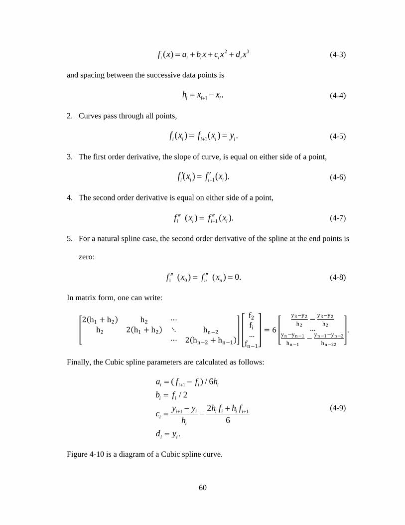
A spline is a function that describes polynomials for formulating a curve. The spline has
been developed and applied in many fields, for example, computer aided design (CAD),
computer aided manufacturing (CAM), computer graphics (CG), and computer vision (CV). A
number of variants have been developed to control the shape of a curve, including Bezier curves,
B-spline, non-uniform rational B-spline (NURBS) and others [Sarfraz 2007].
In this research, the Cubic spline method is applied to the curve lane model. Unlike other
spline models, the Cubic spline passes a set of all N control points and it can use different
boundary conditions for each application.
The following is the Cubic spline condition:
1. Curve model is a third order polynomial:
60
2 3( )i i i i if x a b x c x d x= + + + (4-3)
and spacing between the successive data points is
1 .i i ih x x+= − (4-4)
2. Curves pass through all points,
1( ) ( ) .i i i i if x f x y+= = (4-5)
3. The first order derivative, the slope of curve, is equal on either side of a point,
1( ) ( ).i i i if x f x+′ ′= (4-6)
4. The second order derivative is equal on either side of a point,
1( ) ( ).i i i if x f x+′′ ′′= (4-7)
5. For a natural spline case, the second order derivative of the spline at the end points is
zero:
1 0( ) ( ) 0.n nf x f x′′ ′′= = (4-8)
In matrix form, one can write:
�2(h1 + h2) h2 ⋯
h2 2(h1 + h2) ⋱ hn−2⋯ 2(hn−2 + hn−1)
� �
f2fi…
fn−1
� = 6 �
y3−y2h2
− y3−y2h2…
yn−yn−1hn−1
− yn−1−yn−2hn−22
�.
Finally, the Cubic spline parameters are calculated as follows:
1
1 1
( ) / 6/ 2
26
.
i i i i
i i
i i i i i ii
i
i i
a f f hb f
y y h f h fch
d y
+
+ +
= −
=
− += −
=
(4-9)
Figure 4-10 is a diagram of a Cubic spline curve.
61
Even if a vehicle drives a curved road area, it can be assumed that the vehicle drives in a
straight lane from the local point of view. In many cases, a lane curve line starts from a straight
line and gradually changes its shape to match the curve. Figure 4-11 (C) shows this case. Since
the Canny edge + Hough transform-based first order line solution provides a fairly robust
solution, the Hough transform-based line geometry is a good initial source for finding higher
order line geometry.
Figures 4-9 (B) and 4-11 (B) show the center camera and two camera lane line overlay
image using the Hough transform for a curved road, and Figure 4-12 (B) and (C) shows straight
and curved line results, respectively.
While the Cubic spline is well behaved for a lane curve model representation [Kim 2006,
2009], it is possible to generate an overshot curve because of one or more false intermediate
control points from noise pixels. Therefore, selecting control points is a key step to creating a
lane curve model, so it has to be carefully selected.
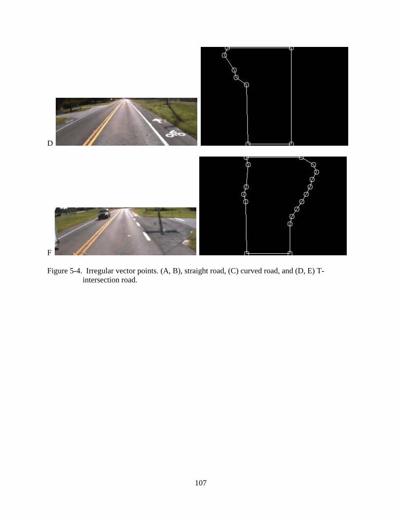
Control Points
Since the Cubic spline passes through all control points, those points have to be selected
precisely. All control points have the same weight; therefore, an incorrectly selected control
point or points can create an erroneous lane model. This problem occurs more at the far side of
an image. In the real world environment, obtaining a clear lane edge filtered image is almost
impossible. Non-lane edge pixels exist randomly by the nature of the world, so the far side of an
image is easily washed out compared to the near side of an image. For this reason, a new control
point selection method is proposed in this dissertation.
The following describes this method:
62
• Normally, a curved line’s start points match the Hough transform line. Therefore, after computing the Hough transform line, N-distance pixels from the Hough line are selected for the curved line candidate’s pixels. Figure 4-12 (A) shows the Canny filtered edge image and Figure 4-12 (B) shows the N-pixel distance area from the Hough transform line. The resulting edge is shown in Figure 4-12 (C).
• The Figure 4-12 (C) image still has many outlier pixels and two lane sides. The greatest size of connected edge pixels is extracted, as shown in Figure 4-12 (D). At this step, only curvature is left to be determined, if a lane is a curved line.
• Next, the normal vectors from the Hough transform line to the curvature pixels and the distance are computed. Based on the image resolution and the real world distance, control points are selected. In Figure 4-12 (F), the blue line shows the normal vectors from the Hough transform line to curvature pixels.
• Finally, the Cubic spline is computed using selected control points.
Lane Model
Because of a property of the Hough transform, many lines, which include not just road lane
lines, but also other lines, are detected, but only lane lines need to be classified [Hashimoto
1992]. Therefore a search method is applied to detect only the two lane lines among the many
line candidates. While line angle and distance parameters are used for this procedure, sometimes
more than two lines meet these line angle and distance conditions. In those cases, the closest line
is selected as the lane line.
Those angle and distance parameters are also employed to verify the lane model
assumption in which the road is modeled as a plane and the lane lines are parallel to each other in
the global view. Also, this lane line model assumption can be applied not only as the vehicle
drives a straight road, but also as the vehicle drives along a curved road. Since the camera field
of view is local and the update rate is around 20Hz, the far area lane correction error caused by a
first order line assumption can be ignored.
63
A global coordinate view, also called a bird’s-eye view, is a good coordinate system for
checking the lane model. Figure 4-14 (A) shows detected lines on a straight road and Figure 4-
14 (B) shows detected lines on a curved road from a bird’s-eye view.
Lane Estimation
In the real world, road conditions may be such that, for a moment, only one or no lane lines
are visible. Even on roads in good repair with proper markings, the problem of losing a lane
reference may occur. This can happen when there is segmented line painting, intersections, or
lane merges. Also, it can happen there is a partial obstruction by another vehicle or there is a
strong shadow on the line on a bright day.
For these instances, an estimation technique is employed to estimate the likely location of
the missing lane boundary line. This is accomplished by using a previous N number of line
parameters that are slope and intersection in the first order line model:
.y mx c= + (4-10)
Eq (4-10) defines a linear line with slope m and intersection c in a Cartesian coordinate
system and (x,y) is the image pixel location.
The linear least-squares estimation technique is applied to estimate a first order lane line’s
angle and intersection parameters. Whenever a lane line is detected, N numbers of line angle and
intersection parameters are stored in a buffer. Then when the vehicle passes the segmented road
line area or crossroad area, those stored parameters are employed for estimating the likely
position of the line. Finally, estimated line parameter’s quality is checked by the lane line model.
If an estimated line meets a lane model, it is used to compute lane correction data. However,
even if the estimated line parameters are good enough to computes lane correction, the estimated
parameters use old data again and again without considering vehicle behavior. Therefore only N-
64
number of the estimated data is processed, otherwise the confidence value is set to zero. Figure
4-15 depicts a line parameter estimation flowchart. This method can be applied without an
accurate vehicle dynamic model [Apolloni 2005].
Let y be the observation vector and N the observation number. The observation vector can
be written as
[ (1),..., ( )]ty y y N= (4-11)
The least square estimate is the value of h that minimizes the square deviation:
( ) ( ) ( ),TJ h y Xh y Xh= − − (4-12)
where X is an N × P matrix where P is the order of the polynomial model of the function.
The solution can be written simply as
1( ) .T Th X X X y−= (4-13)
Figure 4-16 depicts sample results of the lane estimation result. Figure 4-16 (A) and (C)
show two sequential source images from the left camera. Figures 4-16 (B) and (D) show the
detected (blue) line and the estimated (orange) line, when a vehicle passes the segmented line
area. From Figure 4-16, it is clear that the estimation process can effectively determine the
location of the missing boundary and is useful when dealing with segmented lines.
Figure 4-17 shows line angle parameter estimation results. The X axis shows frame
number of sequential images and the Y axis shows the Hough transform line’s angle parameter.
When an autonomous vehicle passes the segmented line area, the lane shows and disappears
again and again. Detected line angle parameters displayed in blue points and estimated line angle
parameters are displayed in orange points.
65
Lane Center Correction
Lane Correction by Two Cameras
Information, such as the estimated center of the current lane combined with lane width, is
used to determine the vehicle orientation within the lane. After converting data from the image
coordinate system to the real world coordinate system, the distances between the
detected/estimated lane lines and the vehicle side are computed (Figure 4-18, purple arrows).
From these distance values, lane correction data (Figure 4-18, blue arrow) and lane width (Figure
4-18, red arrow) are easily computed. Eq (4-14) shows the definition of the lane correction
,R LCorrection d d= − (4-14)
and Eq (4-16) shows how to compute lane width using two distances between the vehicle side
and lane boundary,
.lane L RW d d= + (4-15)
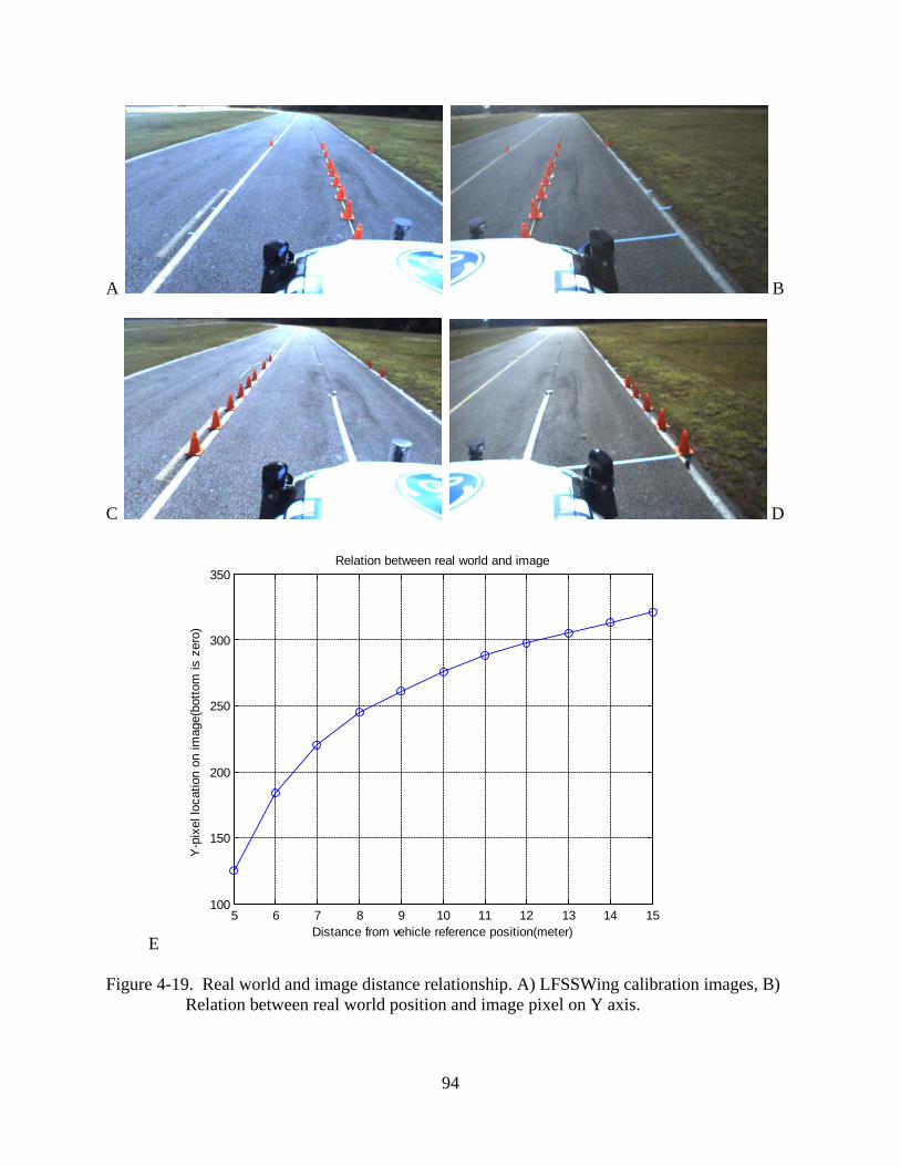
where Wlane is lane width, ande dL , dR is distance between vehicle side and lane boundary. By
the camera calibration, the relationship between the real world distance and the image pixel
distance is measured. Figure 4-19 (A, B, C, and D) shows two camera-based lane finder
calibration images. A resolution at 4, 5, 6, 7, 8, 9, 10, 12 and 14 meters from the vehicle
reference point are summarized in Table 4-2. The resolution at the 5 meter position is around
0.66 centimeters per pixel and at the 7 meter position is around 1 centimeter per pixel.
66
Table 4-2. Two side cameras’ horizontal pixel resolution on 640 x 380 image. Y-
Except for resolution and field of view, the lane correction algorithm is the same as the
LFSSWing algorithm. Lane correction values are computed by using Eq (4-14). These lane
correction values are sent to the LFSS Arbiter component with LFSSWing component correction
values.
Lane Property
Every object color consists of two pieces of color information; real object color and
lighting color. Because of this property, it is not easy to obtain the exact object color in the
outdoor environment in real time. For a moving object, like an autonomous vehicle, lighting
source direction changes over time, so it depends on the surroundings and time of day. For this
reason, color information is not selected as a primary feature in the lane tracking system.
69
However people can acquire more information from not just line type, but also line color. For
example, a vehicle cannot cross the yellow line.
Although it is hard to indentify real object color in the real world. It is not hard to
categorize the line color even if a color source is acquired from an outdoor environment, since
normal painted lane lines are only yellow or white. A histogram matching method using color
pixel distance is proposed to identify lane color. First, lane line mask images are generated using
the bottom part of the image. Because this part includes the most vivid color, high line pixel
resolution and partial lines help it to reduce computation power needs. A part of the detected or
estimated Hough lines are used to generate the mask images. Figure 3-17 shows two camera
field of view mask images.
After generating lane line mask images, the color distance between the lane line color and
each color of the lane color look-up table is calculated using Eq. (4-16).
2 2 2min ( ) ( ) ( ) ,d r r g g b bC p L p L p L= − + − + − (4-16)
where Pr,g,b is the RGB value of lane pixels and Lr,g,b is the RGB value of the look-up table color.
Table 4-6 shows lane color look-up table.
Table 4-6. Lane color look-up table Color Red Green Blue
Yellow 255 255 150
White 255 255 255
Black 0 0 0
70
In this procedure, asphalt color distance is also calculated and then those pixels are ignored
for classifying lane color. Finally, color distance values are utilized for creating a histogram and
deciding the lane color that has the minimum sum of color distances [Krishnan 2007].
Uncertainty Management
The human perception system consists of more than one sensing element, for example,
visual, aural, and tactile senses. Those senses merge together with past experience and using the
brain to make judgments for proper action. In a robotics perception system, the same approach is
demanded because there is no sensor equipment for capturing all sensing information at one time.
Therefore, a sensor fusion process is required in a multiple sensor-based robotic system and each
sensor’s output data management has an important role in this process.
When different types of sensors are tasked with the same goal, the system has to identify
each sensor’s output quality. For example, two different field of view camera systems are
utilized for the lane tracking system and a LADAR-based lane tracking is also developed.
Additionally, even though the vision based lane tracking system gives reliable output in most
cases, there will be occasions when there is the risk of poor or even erroneous output from the
system because of the environment, machine failure, and so on, and these cases need to be
identified.
In addition to the lane tracking outputs, confidence values are provided for uncertainty
management. A root mean square deviation (RMSD) value is used to determine the confidence
value of the lane tracking system output, such as lane center corrections, lane width, and lane
color. The RMSD measures the difference between actual measurement values and predicted
values. In this system, two things are assumed; first, the previous data is the measurement value.
71
Second, the current measurement or estimate data is the predicted value. From this assumption,
the RMSD is calculated as the confidence value using Eq (4-17):
2ˆˆˆRMSD( ) MSE( ) E(( ) ).θ θ θ θ= = − (4-17)
A B
Figure 4-1. Camera field of view diagram. A) The center camera’s view, B) the two side cameras’ view.
72
A
B
C
D
Figure 4-2. Camera field of view. A) Two camera view in an open area, B) two camera view in a traffic area, C) center camera view at the Gainesville Raceway, and D) center camera view when other vehicle blocks a lane.
73
A B
C D Figure 4-3. Canny filtered image samples. A) Original road Image, B) red channel image, C)
Canny filter image with 50/200 threshold value, and D) Canny filter image with 130/200 threshold value.
74
Figure 4-4. Two-camera Canny filtered image in various situations. A) Solid and segmented line, B) segmented line, C) stop line, D) partial block of line, E) curved line, F) noise on the road, G) wipe out line, and H) old tire track on the road.
75
A
B
C
D
E
76
F
G
H
Figure 4-4. Continued.
77
Figure 4-5. Hough space parameters in image coordinate system.
78
A
B
Figure 4-6. Hough space. A) The Canny filtered image at image space, B) A’s Hough space.
Hough Space
θ
ρ
-80 -60 -40 -20 0 20 40 60 80
-600
-400
-200
0
200
400
600
79
Figure 4-7. Hough line transform results. A) Straight road, B) stop line, C) other lines on the middle of the road, D) other lines by noise edge pixel, E) other lines by illumination difference on the road, case I, and F) other lines by illumination difference on the road, case II.
80
A
B
81
C
D Figure 4-7. Continued.
82
E
F Figure 4-7. Continued.
83
Figure 4-8. Lane line checking parameters, angle (Ө) and distance (dL , dR).
84
A
B
Figure 4-9. Center camera results of lane finding with estimated center line. A) Straight road, B) curved road.
85
Figure 4-10. Diagram of Cubic spline and control points.
86
A
B
C
Figure 4-11. Two camera overlay image of lane lines in curved road. A) Straight road, B) crossroad with stop line, and C) curved road.
87
A B
C D
E F
G
Figure 4-12. Hough line + curve control points for spline model.
88
A
B
C
Figure 4-13. Curved lane. A) Source image, B) straight line by the Hough transform, and C) curved line by Cubic spline.
89
A
B
Figure 4-14. Lane model checking view. A) Straight line, B) curved line.
90
Figure 4-15. Line parameter estimation flowchart.
91
A B
C D
Figure 4-16. Two sequence source image and detected (blue) and estimated (orange) line.
92
Figure 4-17. Least squares angle parameter estimation result.
93
A B
Figure 4-18. Lane correction distance definition. A) When a vehicle drives on the left side of the lane, B) when a vehicle drives on the right side of the lane.
94
A B
C D
E
Figure 4-19. Real world and image distance relationship. A) LFSSWing calibration images, B) Relation between real world position and image pixel on Y axis.
5 6 7 8 9 10 11 12 13 14 15100
150
200
250
300
350
Distance from vehicle reference position(meter)
Y-p
ixel
loca
tion
on im
age(
botto
m is
zer
o)
Relation between real world and image
95
Figure 4-20. The LFSS and PFSS calibration image.
96
A
B
C Figure 4-20. Mask images for lane line color. A) Source image, B) Hough transform based line image, and C) mask image.
97
CHAPTER 5 VECTOR-BASED GROUND AND OBJECT REPRESENTATION
Introduction
One of the biggest issues in computer vision systems is the large sizes of the source and
result data. These properties can result in out-sized computation processing, bandwidth
requirement problems, communication delays, and storage issues for an autonomous robot
vehicle, especially systems consisting of multiple components. A recently developed technique,
using computer hardware like general-purpose computing on graphic processing units (GPGPU),
helps to reduce processing time remarkably, but problems still remain. For example, if the robot
system uses a raster-based world representation and sensor data fusion, it requires great storage
space, long computation time, and a large communication bandwidth. It will support only the
specific resolution that is initially defined. However, a vector-based world representation permits
storing, searching, and analyzing certain types of objects using a small storage space. It can also
represent multiple resolution world models that help to improve processing, analyzing, and
displaying the data. In addition, a vector-based system can store much property information in
addition to object information. With these vector-based sensor data representation advantages,
one can store previous traveling information in a database system similar to human memory.
Therefore, one can use previous travel data to verify current travel safety.
Approach
With respect to computation and data storage efficiency, the vector-based representation of
a ground plane is better suited for real-time robot system components. A vector-based
representation can generate both 2-D and 3-D object models with the help of a 3-D sensor like
GPS and LADAR. Specifically, a raster-based world model’s memory size is highly dependent
98
on grid map coverage and resolution. If a world model covers a wide area and is utilized with
high resolution, it needs large computation power and a very large memory space and it causes
bandwidth problem between components. Another issue with a raster-based grid map is that it
contains many areas of unknown data, because the map’s coverage area is fixed. Figure 5-1 (C,
D) shows two different size grid maps from Figure 5-1 (A, B), the source and classified image,
respectively. Figure 5-1(C) is a 241 × 241 size, 0.25 meter resolution grid map, with a data size
56k. And figure 5-1 (D) is a 121×121 size, 0.5 meter resolution grid map, with a data size 14k.
Therefore, raster-based grid map data size depends mostly on the resolution and coverage area.
Table 5-1 summarizes data size of a various format traversability map.
Table 5-1. Raster-based traversability grid map data size Coverage (meter)
Figure 5-5. The TIN representation of traversability map. A) Bird’s-eye view image, B) noise illumination, C) road boundary extraction, D) control point selection, E) 2-D TIN map, and F) 3-D TIN map.
The PFSS, the LFSSWing, and the LFSS software programs were written in C++ for the
Windows environment. Additional functions, algorithms, and GUI are constructed using the
Matrix-Vision API library, and the OpenCV library. Also, the Posix thread library was utilized to
quickly capture the source images from cameras. Both components support the Joint
113
Architecture for Unmanned Systems (JAUS) functionality [JAUS 2009]. JAUS is a
communication protocol that serves to provide a high level of interoperability between various
hardware and software components for unmanned systems. The PFSS, the LFSSWing, and the
LFSS outputs are processed to JAUS messages and sent to the other customer components, for
example, the LFSS Arbiter [Osteen 2008].
Each component provides various intermediate processing results that can be helpful in
running the software parameters or for troubleshooting. For example, the PFSS component
program can display two of the following images: the source image, canny-filtered image, source
image without lane lines, noise-filtered image, or training area image. For the PFSS output, a
raster-based grid map, raster-based grid map without yaw adjustment, road boundary points, or
road polygon image can be selected by the user. Figure 6-3 shows various screenshots of the
PFSS software.
For the LFSSWing and the LFSS, the source image, edge filtered image, Hough line image,
or detected lane line overlay image can be selected. An information window displays each
distance lane center corrections, lane color, and lane width values along with their associated
confidence values. Figure 6-4 shows screenshots of the LFSSWing implementation (the LFSS
software is similar).
The LFSS Arbiter component fuses local roadway data from the TSS, the LFSS, the
LFSSWing, and the Curb Finder smart sensor component [Osteen 2008]. The data consist of
offsets from the centerline of the vehicle to the center of the road lane estimated at varying
distances ahead of the vehicle. Finally, the LFSS Arbiter generates a curve fit from the different
sensor data. These data are used to adjust for GPS measurement errors that are supplied to the
Roadway Navigation (RN) [Galluzzo 2006] component, which navigates the vehicle within a
114
lane using an A* search algorithm. Figure 6-5 (A, B) shows the Gainesville Raceway test area
from the LFSSWing cameras and from a vantage point off of the vehicle, respectively. Figure 6-
5 (C) shows the LFSS Arbiter’s curve fit screen when the vehicle drives along a curved road.
Figure 6-5 (D) shows the Roadway Navigation component’s screenshot of its path searching.
Brown represents the A* search candidate branches and white points are the intermediate goal
points provided from LFSS Arbiter.
Figure 6-6 shows the Urban NaviGator 2009 system architecture. The PFSS, the
LFSSWing, and the World Model Vector Knowledge Store are highlighted. The PFSS stores a
vectorized representation of the road in the WMVKS. The LFSSWing also stores its output as a
vector area that describe lane.
Results
The following section describes the test results pertaining to this research for both the
LFSSWing and the PFSS components. Since the LFSS long range component’s output is very
similar to the LFSSWing component output, the LFSS output is not described in this section.
Based on chapter 2 assumptions, test areas are flat, and the camera source images are clear
enough to see the environment. The auto-exposure control option, which is provided by the
Matrix-vision’s camera setting software, helps to capture a clear source image from various
illumination conditions.
Tests are divided into four categories:
• The Gainesville Raceway,
• The University of Florida campus,
• NW 13th street, and NE 53rd avenue, Gainesville, Florida, and
• Night time setting.
115
The Gainesville Raceway is the only the place to perform an autonomous drive due to a
safety reasons. Since the Gainesville Raceway is a race track, it provides a wide open area and it
does not have standard necessary facilities, such as curbs, pedestrian crossing marks, and so on.
The University of Florida campus provides various urban environment facilities, such as bike
lanes, curbs, pedestrian crossings, sidewalks, more than two lanes, merging or dividing lanes,
and shadows from trees. NW 13th street and NE 53rd avenue are selected to test the software with
traffic and/or at high speeds. The PFSS component was tested only at the Gainesville Raceway
and the University of Florida campus. Finally, the LFSSWing components were tested at night
time with illumination provided from the head lights.
For the autonomous driving tests, vehicle speed was approximately 10 mph. For the real
world tests, vehicle travel speeds were from 20 mph to 60 mph (driven manually). Vector-based
maps were built while traveling approximately 10-20 mph.
LFSSWing test results
The Gainesville Raceway is pictured in the Figure 6-7 (A). The outer loop is
approximately 1 km and the smaller half loop is 650 meters. This course sequence includes a
straight lane, a curved lane, segmented painted lane line, a narrow lane width area, T-intersection
areas, and cross road areas. Since this location is an open area, cameras can receive different
direction’s light in a short time. Figure 6-7 (B) shows a straight lane at the starting point. Figure
6-7 (C) shows a curved lane, with the top part of the right camera source image washed-out due
to the light direction. Figure 6-7 (D) shows that a short length of segmented line can be detected
as a lane line. When the Hough candidate lines are extracted from an edge image (Figure 4-4),
the line length threshold is decided by the source image height. In this research, 20% of source
image height, 48 pixels, is selected as the Hough line minimum length parameter. Figure 6-7 (E)
116
shows a narrow lane compared to a wide lane area in the Gainesville Raceway. The lane width
threshold is defined by a roadway design- plans preparation manual [Florida Department of
Transportation 2009]. 12 feet (3.65 meter) is a standard rural lane width. In this research, a 2 foot
margin is applied, therefore a 10 foot to 14 foot (3.048 meter to 4.267 meter) lane gap is
considered to be a properly detected lane width. The lane width in Figure 6-7 (E) is
approximately 3.35-3.5 meters and it is narrower than a standard lane width. Figure 6-7 (F)
shows a T-intersection area. In this situation, the right lane line is detected and the left lane line
is estimated using previous 20-frames line parameters. Figure 6-7 (G) shows a vehicle traveling
on the right side line in an autonomous test run. Since vehicle controller’s response is not always
fast enough, it is a possibility that the vehicle ventures onto the line momentarily. However,
since lane correction values are being updated continuously, the vehicle can drive back to the
middle of a lane.
The second test place was the University of Florida campus. This location has many
artificial structures, for example bike lanes, curbs, and pedestrian crosswalk and so on. The test
course is an approximately 4 km loop. Figure 6-8 (A) shows a satellite photo of the University of
Florida campus. In Figure 6-8 (B), the LFSSWing operates with shadows in the image. Figure 6-
8 (C) shows a vehicle traveling through a pedestrian crossing area, and figure 6-8 (D) shows the
LFSSWing detecting a curb.
The third test place was an urban area with real traffic. In this environment, sample results
include high speed conditions, divided lane situations, and roads with more than two lanes.
Figure 6-9 shows some urban road test results. Figure 6-9 (A) shows multiple center lane lines,
figure 6-9 (B) shows a divided lane area, and figure 6-9 (C) shows the LFSSWing output with
real traffic on a four-lane road.
117
The fourth test place was the University of Florida campus at night with a nighttime
camera setting. Since illumination is too weak at nighttime, the camera exposure time was
increased and the rest of the LFSSWing setting was the same as daytime. Not just lack of
illumination, but also other artificial lighting sources by other traveling car or streetlight are the
big difference of this test. Figure 6-10 shows various situations outputs in a night time test.
The PFSS test result
The PFSS was tested at the Gainesville Raceway and the University of Florida campus.
Since the PFSS is designed to characterize ground surface area, an urban environment is not
suitable to get meaningful output. For example, if another vehicle travels in the camera’s field of
view, the PFSS possibly considers a vehicle as a non-traversable area. Therefore, the PFSS is
designed and tested in an open area only. Figure 6-11 shows the PFSS test results at the
Gainesville Raceway (see satellite photo in the figure 6-7 (A)). In each case, the source image,
segmented image, and the TIN control points’ image are displayed. Figure 6-11(A) shows a
straight road and Figure 6-11 (B) shows a T-intersection area on the right hand side. In the TIN
control points’ image, the right intersection is identified. Figure 6-11 (C) shows a curved road
with 10 points being used to describe it. Normally, a curved road area needs more points to
represent a ground surface than a straight road area. When a vehicle turns at a T-intersection, a
partial part of road is visible at the camera. Figure 6-11 (D) shows such a situation.
Figure 6-12 shows the University of Florida campus test. Straight road and curved road
cases are shown in Figure 6-12 (A) and (B), respectively. In Figure 6-12 (C), part of the road is
occluded by a bus traveling in the other lane. Therefore representation of the ground surface is
incorrect.
118
Building vector-based map
Both the LFSSWing and the PFSS component’s vector-based lane object and ground
surface maps are reconstructed. In the section, the Gainesville Raceway and the University of
Florida campus are selected as a test environment. Figure 6-7 (A) and Figure 6-8 (A) show each
area’s satellite image.
To generate a lane object vector representation, the lane object is detected, converted from
the local coordinate system to the global coordinate system, and then stored into the WMVKS.
Chapter 4 describes the lane finder algorithm. Figure 6-13 (A, B) shows the vector representation
of a lane at the Gainesville Raceway and at the University of Florida campus, respectively.
For a ground surface vector representation, the ground surface is classified, and road
boundary vector points extracted and converted from the local coordinate system to the global
coordinate system, before being stored into the WMVKS. Chapter 3 describes the path finder
algorithm. Figure 6-14 (A, B) shows the vector representation of the ground surface at the
Gainesville Raceway and at the University of Florida campus, respectively.
Conclusions
The vector-based ground surface and lane objects representation algorithms are
development and implementation to extract and simplify the traversable area by using a camera
sensor. Unlike in simulation, algorithms and methods are engineered for outdoor real-time
applications with continuous and robust output.
This approach allows a robot to have a human-like cognitive system. People feel
comfortable when they drive a known area, because the human brain is able to store important
features by experience. This vision system’s vector output is small enough to be stored and
retrieved like the human brain. Therefore, the vector output can be utilized to rebuild road maps.
119
Also, properties of the road are calculated to better understand the world, such as lane with
and lane color. This information assists the vehicle’s intelligence element in making proper
decisions. All vector data can be stored in a database system in real-time.
Confidence values of output data are also computed. These values play a key role when
data are judged and fused with data from different types of sensor output, such as from LADAR.
It can be fused with vision-based sensor output since all confidence values are normalized.
The author presents results from various test places, time, and conditions. The autonomous
run test verifies that this camera-based lane finder and path finder approach creates robust and
accurate lane corrections, road map, and lane map building. With a simple camera calibration,
this software can be easily deployed to any JAUS system.
Future Work
There are three main areas which could be improved in this research. First, a 3-D model
can be generated using GPS height information and pitch information. Currently, a 2-D model is
generated based on a flat road assumption. However, if this system is used on a slope, hill, or
mountain area, a 3-D road or lane model would provide more accurate information.
Second, the lane line estimator should consider vehicle dynamics. The current estimator
uses previously detected or estimated line parameters to estimate future line parameters without
considering the vehicle’s movement. If vehicle’s yaw information is added to the estimator in
addition to the currently used parameters, the system could generate better estimations,
especially when the vehicle travels through intersection or cross-road areas.
Third, a real-time vector output verification procedure is suggested. This system can store
and build lane and road models. Therefore, if the vehicle re-explores the same area, the system
120
can verify that its current position is within the lane or road by comparing current position with
archived lane or road area information.
121
Figure 6-1. CIMAR Navigator III, Urban NaviGator. A) NaviGator III, B) The front view of NaviGator sensor location, and C) The rear view of NaviGator sensor location.
122
A
B
123
C
Figure 6-1. Continued.
124
A
B
Figure 6-2. NaviGator III camera sensor systems. A) Cameras location. Center camera is shown in red circle and LFSSWing cameras are shown in blue circles, B) Computer system in truck.
125
Figure 6-3. The PFSS software. (A) JAUS service connection windows, (B) source image, (C) edge filtered image, (D) lane mask image, (E) source image over lane mask, (F) training area image, (G) classified image, (H) high resolution bird’s eye view image, (I) boundary candidates point, (J) TIN control points image, (K) 0.25 meter resolution grid-map image without heading, (L) 0.25 meter resolution grid-map image with heading, and (M) information GUI windows
126
A
B C
D E
F G
127
H I
J
K L
Figure 6-3. Continued.
128
M
Figure 6-3. Continued.
129
Figure 6-4. The LFSSWing software A) JAUS service connection windows, B) source image, C) edge filtered image, D) Hough line image, E) detected lane line overlay image, and F) the LFSSWing information window
130
A
B
C
131
D
E
F
Figure 6-4. Continued.
132
A
B
C D
Figure 6-5. The LFSS Arbiter and the RN screen. A) Curved test area, B) different point of view of curved test area, C) the LFSS Arbiter curve fit2 and D) the RN’s A* search result. Brown branches are A* search candidate branch and white points are intermediate travel point by the LFSS Arbiter.
2 This image is generated by Phil Osteen [Osteen 2008].
133
Figure 6-6. Urban NaviGator 2009 system architecture.
134
Figure 6-7. The LFSSWing test result at the Gainesville Raceway. A) Straight lane, B) curved lane, C) segmented lane, D) narrow lane, E) T-intersection lane, and F) when a vehicle drives on the lane line in autonomous run.
135
A
B
C
D
136
E
F
G
Figure 6-7. Continued.
137
Figure 6-8. The LFSSWing test results at the University of Florida campus. A) Satellite photo, B) lane with bike lane in the shadow, C) pedestrian crossing area, and D) curb area.
138
A
B
C
139
D
Figure 6-8. Continued.
140
A
B
C Figure 6-9. The LFSSWing test results in the urban road. A) Multiple center lines, B) divided
lane, C) real traffic situation in four lanes road.
141
A
B
C
D
E
Figure 6-10. The LFSSWing test results at the University of Florida with nighttime setting. A) Straight road, B) other vehicle passed at the other lane, C) other vehicle travel in front of a NiviGator III, D) under a streetlight and E) estimator.
142
Figure 6-11. The PFSS test results in the Gainesville Raceway. Source, segmented and the TIN control points’ images, respectively. A) Straight road, B) T-intersection on right side C) curved road, and D) T-intersection in front.
143
A
B
C
144
D
Figure 6-11. Continued.
145
A
B
C
Figure 6-12. The PFSS test results in the University of Florida campus. Source, segmented and
the TIN control points’ images, respectively. A) Straight road, B) curved road, and C) block by other vehicle.
146
A
B
Figure 6-13. The LFSSWing vector-based representation. A) The Gainesville Raceway (compare to figure 6-7(A) is satellite image), B) the University of Florida campus (compare to figure 6-8 (A) is satellite image).
147
A
B
Figure 6-14. The PFSS vector-based representation. A) The Gainesville Raceway (compare to figure 6-7(A) is satellite image), B) the University of Florida campus (compare to figure 6-8 (A) is satellite image).
148
LIST OF REFERENCES
B. Apolloni, A. Ghosh, F. Alpaslan, L. C. Jain, and S. Patnaik, Machine Learning and Robot Perception (Studies in Computational Intelligence). Berline Heidelberg: Springer, 2005.
R. Behringer, S. Sundareswaran, B. Gregory, R. Elsley, B. Addison, W. Guthmiller, R. Daily, and D. Bevly, "The DARPA grand challenge - development of an autonomous vehicle," in Intelligent Vehicles Symposium, 2004 IEEE, 2004, pp. 226-231.
U. Bergquist, "Colour Vision and Hue for Autonomous Vehicle Guidance," Sweden: Linktping University, 1999.
M. Bertozzi and A. Broggi, "GOLD: a parallel real-time stereo vision system for genericobstacle and lane detection," Image Processing, IEEE Transactions on, vol. 7, pp. 62-81, 1998.
M. Bertozzi and A. Broggi, "Vision-based vehicle guidance," Computer, vol. 30, pp. 49-55, 1997.
S. Beucher and M. Bilodeau, "Road segmentation and obstacle detection by a fast watershed transformation," in Intelligent Vehicles '94 Symposium, Proceedings of the, 1994, pp. 296-301.
T. Bräunl, Embedded Robotics: Mobile Robot Design and Applications with Embedded Systems 3rd ed. Berlin Heidelberg: Springer 2008.
A. Broggi, "Robust real-time lane and road detection in critical shadow conditions," in Computer Vision, 1995. Proceedings., International Symposium on, 1995, pp. 353-358.
A. Broggi and S. Berte, "Vision-based road detection in automotive systems: A real-time expectation-driven approach," Arxiv preprint cs.AI/9512102, 1995.
R. C. Chandler, "Autonomous agent navigation based on textural analysis", Ph.D. dissertation, University of Florida, Gainesville, FL, U.S.A, 2003.
Charles, Martial H. Hebert, Takeo Kanade, 1998, “Vision and Navigation for the Carnegie-Mellon Navlab”, IEEE Transactions on Pattern Analysis and Machine Intelligence. Vol. 10, No. 3, May 1988
J. D. Crisman and C. E. Thorpe, "SCARF: a color vision system that tracks roads and intersections," Robotics and Automation, IEEE Transactions on, vol. 9, pp. 49-58, 1993.
E. R. Davies, Machine Vision : Theory, Algorithms, Practicalities (Signal Processing and its Applications). San Franscisco, CA: Morgan Kaufmann, 2004.
I. L. Davis, A. Kelly, A. Stentz, and L. Matthies, "Terrain typing for real robots," in Intelligent Vehicles '95 Symposium., Proceedings of the, 1995, pp. 400-405.
149
R. O. Duda, P. E. Hart, and D. G. Stork, Pattern Classification, 2nd ed. New York: Willy-Interscience, 2000.
R. O. Duda and P. E. Hart, "Use of the Hough transformation to detect lines and curves in pictures," Commun. ACM, vol. 15, pp. 11-15, 1972.
Florida Department of Transportation, Roadway design, “Plans Preparation Manual- Jan 2009 update, Volume 1 – Design Criteria and Process”, January, 2009, http://www.dot.state.fl.us/rddesign/PPMManual/2009/Volume1/2009Vol1.shtm,2009
D. W. Gage, "A brief history of unmanned ground vehicle (UGV) development efforts," Unmanned Systems, vol. 13, pp. 9-32, 1995.
R. C. Gonzalez, R. E. Woods, and S. L. Eddins, Digital Image Processing Using MATLAB. New Jersey: Prentice Hall, 2004.
T. Galluzzo, "Simultaneous Planning and Control for Autonomous Ground Vehicles.", Ph.D. dissertation, University of Florida, Gainesville, FL., U.S.A, 2006.
R. Hartley and A. Zisserman, Multiple View Geometry in Computer Vision. Cambridge, UK: CAMBRIDGE UNIVERSITY PRESS, 2004.
K. Hashimoto, S. Nakayama, T. Saito, S. Ishida, K. Unuora, J. Ishii, N. Oono, and Y. Okada, "An image processing architecture and a motion control method for an autonomous vehicle," in Intelligent Vehicles '92 Symposium., Proceedings of the, 1992, pp. 213-218.
M. Isard and A. Blake, "CONDENSATION—Conditional Density Propagation for Visual Tracking," International Journal of Computer Vision, vol. 29, pp. 5-28, 1998.
JAUS Working Group, "Joint Architecture for Unmanned Systems(JAUS)", http://www.jauswg.org/,2009
J. C. McCall and M. M. Trivedi, "Video-based lane estimation and tracking for driver assistance: survey, system, and evaluation," IEEE Transactions on Intelligent Transportation Systems, vol. 7, pp. 20-37, 2006.
A. Kelly and A. Stentz, "An approach to rough terrain autonomous mobility," in International Conference on Mobile Planetary Robots, 1998, pp. 129-198.
Z. Kim, "Realtime lane tracking of curved local road," in Intelligent Transportation Systems Conference, 2006. ITSC '06. IEEE, 2006, pp. 1149-1155.
Z. Kim, "Robust Lane Detection and Tracking in Challenging Scenarios," Intelligent Transportation Systems, IEEE Transactions on, vol. 9, pp. 16-26, 2008.
K. Kluge, "Extracting road curvature and orientation from image edge points without perceptual grouping into features," in Intelligent Vehicles' 94 Symposium, Proceedings of the, 1994, pp. 109-114.
150
K. Kluge and S. Lakshmanan, "A deformable-template approach to lane detection," in Intelligent Vehicles '95 Symposium., Proceedings of the, 1995, pp. 54-59.
C. Kreucher and S. Lakshmanan, "LANA: a lane extraction algorithm that uses frequency domain features," Robotics and Automation, IEEE Transactions on, vol. 15, pp. 343-350, 1999.
Krishnan, N., Banu, M. S. and Christiyana, C. C. “Content Based Image Retrieval Using Dominant Color Identification Based on Foreground Objects”, City, 2007.
J. Lee and C. D. Crane, "Road Following in an Unstructured Desert Environment Based on the EM(Expectation-Maximization) Algorithm," in SICE-ICASE, 2006. International Joint Conference, 2006, pp. 2969-2974.
J. W. Lee, "A machine vision system for lane-departure detection," Comput. Vis. Image Underst., vol. 86, pp. 52-78, 2002.
Lukac, R. and K.N. Plataniotis, "Color Image Processing: Methods and Applications". 2006, Boca Raton, FL: CRC Press.
Matrix Vision, "The mvBlueFOX USB 2.0 camera", http://www.matrix-vision.com/products/hardware/mvbluefox.php?lang=en,2009
L. Matthies, M. Maimone, A. Johnson, Y. Cheng, R. Willson, C. Villalpando, S. Goldberg, A. Huertas, A. Stein, and A. Angelova, "Computer Vision on Mars," International Journal of Computer Vision, vol. 75, pp. 67-92, 2007.
J. C. McCall and M. M. Trivedi, "Video-based lane estimation and tracking for driver assistance: survey, system, and evaluation," IEEE Transactions on Intelligent Transportation Systems, vol. 7, pp. 20-37, 2006.
H. P. Moravec, "The Stanford Cart and the CMU Rover," Proceedings of the IEEE, vol. 71, pp. 872-884, 1983.
M. Nixon and A. S. A. A. (Author), Feature Extraction in Computer Vision and Image Processing, 2nd ed. Oxford, UK: Elsevier, 2008.
P. Osteen, "Local Sensor Data Fusion Applied to Autonomous Navigation", M.S. thesis, University of Florida, Gainesville, Fl., U.S.A, 2008.
D. Pomerleau, "RALPH: Rapidly adapting lateral position handler," in IEEE symposium on intelligent vehicles, 1995, pp. 506-511.
D. Pomerleau and T. Jochem, "Rapidly adapting machine vision for automated vehicle steering," IEEE Expert, vol. 11, pp. 19-27, 1996.
151
C. Rasmussen, "Combining laser range, color, and texture cues for autonomous road following," in Robotics and Automation, 2002. Proceedings. ICRA'02. IEEE International Conference on, 2002.
M. Sarfraz, Interactive Curve Modeling: with Applications to Computer Graphics, Vision and Image Processing London, UK: Springer-Verlag, 2007.
H. Schneiderman and M. Nashman, "A discriminating feature tracker for vision-based autonomous driving," Robotics and Automation, IEEE Transactions on, vol. 10, pp. 769-775, 1994.
S. Solanki, "Development of Sensor Component for Terrain Evaluation and Obstacle Detection for an Unmanned Autonomous Vehicle", Ph.D. dissertation, University of Florida, Gainesville, Fl., U.S.A, 2006.
B. Southall and C. J. Taylor, "Stochastic road shape estimation," in International Conference on Computer Vision, 2001, pp. 205-212.
R. Sukthankar, D. Pomerleau, C. Thorpe, and I. Carnegie-Mellon Univ Pittsburgh Pa Robotics, Panacea: An Active Sensor Controller for the ALVINN Autonomous Driving System: Carnegie Mellon University, The Robotics Institute, 1993.
T. Suttorp and T. Bucher, "Learning of Kalman Filter Parameters for Lane Detection," in Intelligent Vehicles Symposium, 2006 IEEE, 2006, pp. 552-557.
C. J. Taylor, J. Kosecka, R. Blasi, and J. Malik, "A comparative study of vision-based lateral control strategies for autonomous highway driving," The International Journal of Robotics Research, vol. 18, p. 442, 1999.
C. Thorpe, M. Hebert, T. Kanade, and S. Shafer, "Vision and Navigation for the Carnegie-Mellon Navlab," Annual Reviews in Computer Science, vol. 2, pp. 521-556, 1987.
S. Thrun, M. Montemerlo, H. Dahlkamp, D. Stavens, A. Aron, J. Diebel, P. Fong, J. Gale, M. Halpenny, and G. Hoffmann, "Stanley: The robot that won the DARPA Grand Challenge," JOURNAL OF FIELD ROBOTICS, vol. 23, p. 661, 2006.
R. Touchton, "An Adaptive Planning Framework for Situation Assessment and Decision-Making of an Autonomous Ground Vehicle.", Ph.D. dissertation, University of Florida, Gainesville, FL., U.S.A, 2006.
S. J. Velat, J. Lee, N. Johnson, and C. D. Crane, "Vision Based Vehicle Localization for Autonomous Navigation," in Computational Intelligence in Robotics and Automation, 2007. CIRA 2007. International Symposium on Jacksonville, FI 2007, pp. 528-533
V. Vezhnevets, V. Sazonov, and A. Andreeva, "A Survey on Pixel-Based Skin Color Detection Techniques," in Proc. Graphicon, 2003.
152
Y. Wang, D. Shen, and E. K. Teoh, "Lane detection using catmull-rom spline," in IEEE International Conference on Intelligent Vehicles, 1998.
Y. Wang, D. G. Shen, and E. K. Teoh, "Lane detection using spline model," Pattern Recognition Letters, vol. 21, pp. 677-689, Jul 2000.
Y. Wang, E. K. Teoh, and D. G. Shen, "Lane detection and tracking using B-Snake," Image and Vision Computing, vol. 22, pp. 269-280, Apr 1 2004.
C. Witzgall, J. Bernal, and G. S. Cheok, "TIN Techniques for Data Analysis and Surface Construction," National Institute of Standards and Technology Internal Report 7078, 2004, 2004.
B. F. Wu, C. T. Lin, and Y. L. Chen, "Dynamic Calibration and Occlusion Handling Algorithms for Lane Tracking," Ieee Transactions on Industrial Electronics, vol. 56, pp. 1757-1773, May 2009.
Y. U. Yim and S. Y. Oh, "Three-feature based automatic lane detection algorithm (TFALDA) for autonomous driving," IEEE Transactions on Intelligent Transportation Systems, vol. 4, pp. 219-225, 2003.
Yu, X., S. Beucher, and M. Bilodeau. "Road tracking, lane segmentation and obstacle recognition by mathematical morphology". in Intelligent Vehicles '92 Symposium., Proceedings of the. 1992.
J. Zhang and H. H. Nagel, "Texture-based segmentation of road images," in Intelligent Vehicles' 94 Symposium, Proceedings of the, 1994, pp. 260-265.
153
BIOGRAPHICAL SKETCH
Jaesang Lee was born and raised in Seoul, Korea. He completed his Bachelor of Science
degree in an Electrical Engineering Department at the Inha University in Inchon, Korea, and
began his Master of Science degree at Inha University. After finishing military duty at the Air
Force, Jaesang decided to go back to school to finish his master’s degree in the United States. He
finished his master’s program in Electrical and Computer Engineering Department at the
University of Florida and then joined his Ph.D. program at the Center for Intelligent Machines
and Robotics (CIMAR) in the Mechanical and Aerospace Engineering Department. Jaesang has
worked on various robotics projects as a graduate research assistant under the guidance of his
advisor, Dr. Carl D. Crane III. Among the projects, Jaesang was actively involved in the
autonomous vehicle development for the Defense Advanced Research Projects Agency (DARPA)
Grand Challenge 2005 and DARPA Urban Challenge 2007. His current research goal is
computer vision system development for autonomous vehicle and drive assistant system. After
graduation, Jaesang will continue his career as an engineer working in the robotics industry. His
field of interest includes computer vision, image processing, and pattern recognition system