Vendor managed inventory in tramp shipping Magnus Stålhane a,n , Henrik Andersson a , Marielle Christiansen a , Kjetil Fagerholt a,b a Norwegian University of Science and Technology, Department of Industrial Economics and Technology Management, Alfred Getz vei 3, NO-7491 Trondheim, Norway b Norwegian Marine Technology Research Institute (MARINTEK), Otto Nielsens veg 10, NO-7052 Trondheim, Norway article info Article history: Received 23 November 2012 Accepted 14 March 2014 Processed by B. Lev Available online 25 March 2014 Keywords: Vehicle scheduling Routing Inventory management Integer programming abstract This paper introduces a new problem to the OR community that combines traditional tramp shipping with a vendor managed inventory (VMI) service. Such a service may replace the more traditional contract of affreightment (COA) which for decades has been the standard agreement between a tramp shipping company and a charterer. We present a mathematical formulation describing the routing and scheduling problem faced by a tramp shipping company that offers a VMI service to its customers. The problem is formulated as an arc-flow model, and is then reformulated as a path-flow model which is solved using a hybrid approach that combines branch-and-price with a priori path-generation. To solve larger, and more realistic, instances we present a heuristic path-generation algorithm. Computational experiments show that the heuristic approach is much faster than the exact method, with insignificant reductions in solution quality. Further, we investigate the economic impact of introducing a VMI service, by comparing the results obtained with the new model with results obtained by solving the traditional routing and scheduling problem faced by tramp shipping companies using COA. The computational results show that it is possible to substantially increase supply chain profit and efficiency by replacing the traditional COAs with VMI services. & 2014 Elsevier Ltd. All rights reserved. 1. Introduction Maritime transportation has for centuries been the only viable way of transporting large quantities of goods between continents. However, as the competition in international shipping is getting fiercer, several traditional tramp shipping companies are looking to expand their service portfolio to attract new customers and gain a competitive advantage. One such type of logistics service is inventory management. This type of service has been offered for some time by land-based transportation companies, a service often referred to as vendor managed inventory (VMI), see for instance Day et al. [12]. VMI transfers the management of inven- tories and order processing from the buyer of a product to the supplier of the product. A well known example of this is super- markets; rather than managing their own inventories, they now let each supplier manage the inventory of their products. However, VMI may also refer to business models where a third party logistics provider manages the inventory of the buyer, the supplier, or both, and it is this type of VMI service that some traditional tramp shipping companies are now considering. To the authors' knowledge, there exists only a couple of instances where shipping companies have offered this type of service to a customer. The main barrier that needs to be overcome in order to introduce a VMI service on a larger scale in the tramp shipping industry is that the shipping industry in general is a conservative industry where secrecy is often considered impor- tant. Both charterers (cargo owners) and shipping companies have for decades had a business model where a competitive advantage was gained by having better, and more up to date, knowledge than their competitors. In addition, third party brokers have made a living for themselves by taking the role as middle men in transactions between charterers and shipping companies because neither side has been willing to share information. However, in an age where information is readily available, it is becoming much harder to gain a competitive advantage based on knowledge of the market. Thus, the shipping industry needs to start taking advan- tage of the capabilities provided by information technology and share information with their customers. In the context of maritime transportation, VMI services will first and foremost replace the traditional contract of affreightment (COA), which is a contract entered into by a charterer and the shipping company. In a COA the shipping company agrees to transport a series of cargoes between a loading and an unloading port for a fixed price per ton [31]. Usually, such contracts also include clauses that the shipments or cargoes should be fairly Contents lists available at ScienceDirect journal homepage: www.elsevier.com/locate/omega Omega http://dx.doi.org/10.1016/j.omega.2014.03.004 0305-0483/& 2014 Elsevier Ltd. All rights reserved. n Corresponding author. Tel.: +47 73 59 3511. E-mail address: [email protected](M. Stålhane). Omega 47 (2014) 60–72
Transcript
Vendor managed inventory in tramp shipping
Magnus Stålhane a,n, Henrik Andersson a, Marielle Christiansen a, Kjetil Fagerholt a,b
a Norwegian University of Science and Technology, Department of Industrial Economics and Technology Management, Alfred Getz vei 3,NO-7491 Trondheim, Norwayb Norwegian Marine Technology Research Institute (MARINTEK), Otto Nielsens veg 10, NO-7052 Trondheim, Norway
a r t i c l e i n f o
Article history:Received 23 November 2012Accepted 14 March 2014Processed by B. LevAvailable online 25 March 2014
This paper introduces a new problem to the OR community that combines traditional tramp shippingwith a vendor managed inventory (VMI) service. Such a service may replace the more traditionalcontract of affreightment (COA) which for decades has been the standard agreement between a trampshipping company and a charterer. We present a mathematical formulation describing the routing andscheduling problem faced by a tramp shipping company that offers a VMI service to its customers. Theproblem is formulated as an arc-flow model, and is then reformulated as a path-flow model which issolved using a hybrid approach that combines branch-and-price with a priori path-generation. To solvelarger, and more realistic, instances we present a heuristic path-generation algorithm. Computationalexperiments show that the heuristic approach is much faster than the exact method, with insignificantreductions in solution quality. Further, we investigate the economic impact of introducing a VMI service,by comparing the results obtained with the new model with results obtained by solving the traditionalrouting and scheduling problem faced by tramp shipping companies using COA. The computationalresults show that it is possible to substantially increase supply chain profit and efficiency by replacingthe traditional COAs with VMI services.
& 2014 Elsevier Ltd. All rights reserved.
1. Introduction
Maritime transportation has for centuries been the only viableway of transporting large quantities of goods between continents.However, as the competition in international shipping is gettingfiercer, several traditional tramp shipping companies are lookingto expand their service portfolio to attract new customers and gaina competitive advantage. One such type of logistics service isinventory management. This type of service has been offeredfor some time by land-based transportation companies, a serviceoften referred to as vendor managed inventory (VMI), see forinstance Day et al. [12]. VMI transfers the management of inven-tories and order processing from the buyer of a product to thesupplier of the product. A well known example of this is super-markets; rather than managing their own inventories, they now leteach supplier manage the inventory of their products. However,VMI may also refer to business models where a third party logisticsprovider manages the inventory of the buyer, the supplier, or both,and it is this type of VMI service that some traditional trampshipping companies are now considering.
To the authors' knowledge, there exists only a couple ofinstances where shipping companies have offered this type ofservice to a customer. The main barrier that needs to be overcomein order to introduce a VMI service on a larger scale in the trampshipping industry is that the shipping industry in general is aconservative industry where secrecy is often considered impor-tant. Both charterers (cargo owners) and shipping companies havefor decades had a business model where a competitive advantagewas gained by having better, and more up to date, knowledge thantheir competitors. In addition, third party brokers have madea living for themselves by taking the role as middle men intransactions between charterers and shipping companies becauseneither side has been willing to share information. However, in anage where information is readily available, it is becoming muchharder to gain a competitive advantage based on knowledge of themarket. Thus, the shipping industry needs to start taking advan-tage of the capabilities provided by information technology andshare information with their customers.
In the context of maritime transportation, VMI services willfirst and foremost replace the traditional contract of affreightment(COA), which is a contract entered into by a charterer and theshipping company. In a COA the shipping company agrees totransport a series of cargoes between a loading and an unloadingport for a fixed price per ton [31]. Usually, such contracts alsoinclude clauses that the shipments or cargoes should be fairly
Contents lists available at ScienceDirect
journal homepage: www.elsevier.com/locate/omega
Omega
http://dx.doi.org/10.1016/j.omega.2014.03.0040305-0483/& 2014 Elsevier Ltd. All rights reserved.
evenly spread over the contract period, which is used to derivetime windows for when the shipping company must start loadingand unloading the cargoes. The quantities of the cargoes are alsospecified in the COAs. Frequently, these quantities are specifiedwithin an interval, for example 50,000710% tons. There are twomain types of COAs with such flexible quantities; MOLOO (more orless owner's option) and MOLCO (more or less charterer's option).In MOLCO contracts the charterer decides the exact quantity ofeach cargo from an interval stated in the COA. Often this decisionis not made until the ship arrives at the loading port, and thus theshipping company has to plan for the maximum allowed quantityto be loaded. In MOLOO contracts it is the shipping company thatdecides the cargo quantity transported from the interval statedin the COA. Both the time windows and the quantity intervalsare terms decided on during contract negotiations. Generally forMOLOO contracts, the wider this interval is, the lower price perton can be expected since widening this interval gives the shippingcompany more planning flexibility, while the reverse is true forMOLCO contracts [6].
However, in many cases the real situation is that the chartereris responsible for storages at both the loading and unloading ports.The loading port is often located by a facility producing theproduct, while the unloading port can be considered as a con-sumption port. Hence, the charterer needs to ship the productfrom the loading to the unloading port in order to maintainfeasible inventory levels at both storages. Lack of transparencyand communication between charterers and shipping companieshas led to the abovementioned COAs. Both MOLOO and MOLCOcontracts create uncertainty in the operations for one of theparties that enters into the COA, because it does not know theexact quantity that is to be loaded and unloaded during a visit to aport. This uncertainty creates a risk to which the charterer/shipping company assigns a risk premium. Thus, shipping compa-nies charge a higher price to MOLCO contracts where theyincur the risk, while the charterers demand a lower price forMOLOO contracts where they are taking the risk. With thecapabilities of information technology today, much of this riskcan be removed by introducing a VMI service that can replace theCOAs. Such a VMI service gives the shipping company fulltransparency of the charterer's storages, resulting in more plan-ning flexibility for the shipping company regarding both thequantity and the timing of a shipment. In addition, it gives thecharterer lower operational costs as they do not have to do orderprocessing and handling. In total this could result in lower supplychain costs.
The contribution of this paper to the research community isthreefold. First, we present a new problem to the literature, wheretraditional COAs are combined with VMI services, and present adetailed mathematical model of the problem. Second, we present anew solution approach based on branch-and-price that is able tosolve realistic instances of the problem, both exactly and heuristically.Third, we analyze the economic impact for the shipping company,and the supply chain, from replacing some of the traditional COAswith VMI services. As COAs usually state that the product is to betransported between one loading port and a corresponding unload-ing port, it would be a natural first step for a tramp shippingcompany to offer a VMI service where the storages are paired. Thus,all cargoes transported from one producing storage have to bedelivered to the corresponding consuming storage. The tramp ship-ping company must ensure that the inventories of all storages staywithin their limits by transporting the products between theproduction ports and the corresponding consumption ports. Further-more, the tramp shipping company is also engaged in transportingcargoes on the spot market and will choose to carry such optionalcargoes if there is sufficient fleet capacity and they are profitable. Toinvestigate the economic impact a shipping company may incur
by offering this new type of VMI service, we present mathematicalmodels both of the VMI service and a more traditional service usingCOAs. The two types of services are compared by solving the modelson the same set of instances.
We use the definition from Al-Khayyal and Hwang [1] anddistinguish between cargo routing and inventory routing. We usecargo routing to denote the planning problem of routing a fleet ofships to service a number of specified cargoes, with givenquantities (or quantity intervals) and time windows that are givenas input to the planning process (from COAs or the spot market).This is in contrast to inventory routing where the cargoes (from theVMI contracts) are determined by the planning process itself. Theresulting planning problem that we consider in this paper is acombined cargo and inventory routing problem faced by a ship-ping company that offers VMI services to some of its customersand is also engaged in transporting COA cargoes and optional spotcargoes. This combined cargo and inventory routing problem withpaired inventories has to the authors' knowledge not been studiedin the research literature previously.
The cargo routing and scheduling problem faced by trampshipping companies is a maritime adaptation of the more generalpickup and delivery problemwith timewindows (PDPTW), describedby, among others, Desrosiers et al. [13], and surveyed by Berbegliaet al. [4]. What characterizes the maritime version of the PDPTW isthat the fleet of ships is heterogeneous, and no common depot exists.The planning horizon and travel times are longer, and the cargoquantities are usually large compared with the size of the ships.There is also normally a mix of mandatory contracted cargoesand optional spot cargoes. The maritime PDPTW has been studiedby, among others, Brønmo et al. [5], Korsvik et al. [20] and Malliappiet al. [24], who all propose heuristic solution methods to theproblem. Several extensions of the maritime PDPTW have beenintroduced in recent years. Among these are Brønmo et al. [6] whointroduce MOLOO contracts in the form of flexible cargoes, where theshipping company may choose the quantity of each cargo to pick upwithin given intervals. In contrast to the problem considered in thispaper, the above studies only deal with cargo routing problemswithout any inventory management.
Inventory considerations in maritime transportation most oftenoccur in vertically integrated companies, where the same companycontrols all inventories as well as the fleet of ships transportingthe products. The basic maritime inventory routing problem (MIRP)consists of a single product that is to be transported from a set ofproduction ports to a set of consumption ports in such a way that theinventory limits are respected at all ports. This problem has beenstudied by, among others, Christiansen [8], Christiansen and Nygreen[11], Song and Furman [29] and Engineer et al. [14]. The first twopapers consider problems where the production/consumption ratesare constant, and use a continuous time formulation, while the lattertwo have production/consumption rates that vary over the planninghorizon and use discrete time models. A common extension of theMIRP is to include multiple products. This is done by, for instance,Ronen [27], Persson and Göthe-Lundgren [26], Khayyal and Hwang[1], and Christiansen et al. [9]. The inventory part of the problemstudied in this paper may be viewed as a special case of a multi-product MIRP where each product has exactly one production andone consumption port. None of the above studies on maritimeinventory routing includes paired inventories, like the problemstudied in this paper.
The rest of the paper is organized as follows: in Section 2 wegive a more formal description of the problem, and present anarc-flow formulation. Further, we present a reformulation of theproblem together with our solution approach in Section 3, beforeSection 4 describes how the contracts of affreightment are modeled.Finally, we present our computational study in Section 5, beforeoffering some concluding remarks in Section 6.
M. Stålhane et al. / Omega 47 (2014) 60–72 61
2. Problem description and formulation
This section presents a more detailed description of the com-bined cargo and inventory routing problem considered in thispaper. In Section 2.1, we give a description of the routing andscheduling problem faced by a tramp shipping company that offersa VMI service, before an arc-flow formulation of the problem ispresented in Section 2.2. The arc-flow formulation is presented togive a detailed description of the problem studied.
2.1. Problem description
The problem studied in this paper contains a set of transporta-tion tasks, C¼ f1;…;Ng, that may be divided into three categories:mandatory cargoes (CM) that have to be serviced, optional cargoes(CO) that may be serviced, and inventory pairs (CI) that may beserviced a number of times to keep the inventories within theirlimits. We define the problem on a graph G¼ ðN ;AÞ where N isthe set of nodes, and A is the set of arcs. Let each node in N bedenoted (i,m) where iAf1;…;2Ng and mAMi ¼ f1;…;Mig whereMi is an upper bound on the number of times transportation task i(or i�N) may be serviced.
N can be divided into two disjoint sets. Let N P ¼ fði;mÞ :i¼ 1;…;N and mAMig be the set of loading nodes, one for eachloading port and visit number of transportation task i, and letN D ¼ fði;mÞ : i¼Nþ1;…;2N and mAMig be the set of unloadingnodes, one for each unloading port and visit number of transpor-tation task i�N. The set N can also be divided into three disjointsets, N C which are nodes associated with contracted cargoes,N O which are nodes associated with optional (or spot) cargoes,and N I which are nodes associated with inventory pairs. Foroptional and mandatory cargoes Mi ¼ 1, while the inventory pairsmay be serviced more than once. Note that Mi ¼M ðNþ iÞ since thenumber of loadings and unloadings must be the same for allinventory pairs. Each transportation task earns the shippingcompany a revenue Ei for performing that task. The start of serviceat each node (i,m) is constrained by a time window, denoted½T im; T im�.
The fleet available is heterogeneous and considered fixedduring the planning horizon which starts at time 0 and endsat time T. The set of ships V is indexed by v. Each ship v has acapacity Kv, a starting position o(v), an artificial ending position d(v), and a graph Gv ¼ ðN v;AvÞ associated with it. The set of verticesN vDN P [ N D [ fðoðvÞ;1Þ; ðdðvÞ;1Þg, and the set of arcs Av �N v �N v define the feasible movements for ship v. Each arc, ðði;mÞ; ðj;nÞÞ,represents ship v sailing from node (i,m) to node (j,n) andassociated with the arc there is a corresponding non-negativecost Cijv and traveling time Tijv.
For each node ði;mÞAN C [ N O there is an associated cargoquantity Qi that must be transported from the loading port to theunloading port. Each node ði;mÞAN I is associated with a storage iwith a maximum inventory level Si, a minimum inventory level Si,an initial inventory level Si, and a production (if positive) andconsumption (if negative) rate Ri. There is also a minimum andmaximum limit on the quantity that may be loaded/unloaded,denoted Q
iand Q i, respectively. The visit number m to an
inventory node defines the order in which the visits are made,so that node (i,m) is serviced before node ði;mþ1Þ. With each nodei there is an associated loading/unloading rate Ti
Q, denoting howmuch time it takes to load/unload one unit of cargo at that node.
In the reminder of this paper we use the term route to denote apath for ship v from ðoðvÞ;1Þ to ðdðvÞ;1Þ in Gv. The route is feasible iffor each loading node (i,m) visited, the corresponding unloadingnode ðNþ i;nÞ is visited afterwards, the capacity of the ship isnever violated and the time windows are respected at every node.The objective is to create a set of routes, one for each ship, such
that the total profit of the fleet is maximized, while satisfying allthe constraints mentioned above.
2.2. Arc-flow model
Let variable ximjnv be equal to 1 if ship v sails directly from node(i,m) to node (j,n), and 0 otherwise, and let yim be equal to 1 if node(i,m) is not visited, and 0 otherwise. Variable limv representsthe amount of cargo onboard ship v after leaving node (i,m), timrepresents the time service is started at node (i,m), and qim denotesthe amount of cargo loaded or unloaded at node (i,m). Theinventory level at inventory i at the start of service for visit m isgiven by sim, and wimnv is equal to 1 if the inventory cargo loaded atnode (i,m) is unloaded at node ðNþ i;nÞ using ship v, and 0 other-wise. The coefficient Ii is equal to 1 if node (i,m) is a loading node,and �1 if it is a unloading node. Finally, let si denote the inventorylevel at storage i at the end of the planning horizon. The arc-flowmodel of the problem may then be formulated as follows:
wimnvAf0;1g; 8vAV; ði;mÞAN P ; nAMðNþ iÞ: ð35ÞThe objective function (1) maximizes the profit of the shippingoperations. The first term of the objective function sums up therevenues from servicing the inventory and mandatory cargoeswhile the second term adds the revenue from the optional cargoesthat are serviced. The third term subtracts the total sailing costs ofthe fleet of ships.
Constraints (2)–(4) conserve the flow through the network,while constraints (5) ensure that both the loading and unloadingnodes of a non-inventory cargo are visited by the same ship.Further, constraints (6)–(8) state that all contractual cargoes areserviced once, while all optional cargoes and inventory nodesare serviced at most once. The cargo quantity onboard the shipon each arc in the network is managed by constraints (9), andconstraints (10) ensure that the load onboard the ship is betweenzero and the capacity of the ship. Constraints (11) set an upper anda lower limit on the cargo quantity (un)loaded at each visit toan inventory node, while constraints (12) fix the optional andmandatory cargo quantity variables.
Constraints (13) keep track of the start of service at each node,while constraints (14) ensure that each loading node is visitedbefore the corresponding unloading node. Note that even thoughloading node (i,m) and unloading node ðNþ i;mÞ are not necessa-rily visited by the same ship, this relationship still holds. Theservice time variables for mandatory and optional cargoes are keptbetween their upper and lower bounds by constraints (15). Toensure that the inventory constraints are still correct if the nodeis not serviced, constraints (16) force the time variables to beequal to the end of the planning horizon if the inventory node is
not serviced, and between its upper and lower bound otherwise.Constraints (17) state that the chronological order of visits to eachinventory happens in numerical order.
The inventory levels at the start of service at each visit to aninventory node are controlled by constraints (18) and (19). Con-straints (20) and (21) ensure that the inventory levels are stillfeasible at the end of each visit, and at the end of the planninghorizon, while constraints (22) and (23) make sure that theinventory levels are between their upper and lower limits.
Constraints (24) and (25) ensure that there is at most oneconnection between a loading node and an unloading node, whileconstraints (26) and (27) state that the variables connecting aloading and an unloading node can only be equal to one if the shipvisits both nodes. Constraints (28) make sure that the volumeloaded and unloaded at both nodes are the same, and constraints(29) ensure that the pickup node is visited before the deliverynode also for inventory cargoes. Constraints (30) enforce that if aninventory node is visited, then so are all the inventory nodes witha smaller visit number, and constraints (31) say that if the loadingnode with a given visit number is not visited, then neither is thecorresponding unloading node with the same visit number. Finally,constraints (32) set the start time of the route to zero, whileconstraints (33)–(35) put binary restrictions on the artificial visitand arc-flow variables.
3. Reformulation and solution approach
Arc-flow models are well suited to describe the details of aproblem. However, they usually perform inferior to path-flowmodels due to the large number of constraints and a relativelyweak linear programming (LP) bound. This has been shown by,among others, Grønhaug and Christiansen [17] for a maritimeinventory routing problem, Andersson et al. [2] and Norstad et al.[25] for two other maritime transportation problems, and Røpkeand Cordeau [28] for a land-based PDPTW. Initial testing of ourarc-flow model supports these findings. Thus, to test the perfor-mance of VMI we reformulate the problem as a path-flow model.This model, hereafter referred to as the VMI model, is describedin Section 3.1. To solve the VMI model we present a solutionapproach based on branch-and-price. The details of this solutionapproach are described in Section 3.2.
3.1. VMI model
To present the VMI model we need to define some additionalnotation. The set Rv, indexed by r, contains all routes for a givenship v. Associated with a route there is a cost Cvr defined as thesum of the arc costs of sailing route r with ship v, and coefficientsAimvr which are equal to 1 if route r of ship v includes node (i,m),and 0 otherwise. The set Wr , indexed by w, is the set of allschedules for route r. A schedule contains the exact time for startof service and the exact quantity picked up or delivered at eachnode visited on the given route. Note that for a given route thereexists an infinite number of feasible schedules. Let Timvrw andQimvrw denote the time service is started, and the quantity pickedup, or delivered, at node (i,m) by ship v sailing route r and usingschedule w, respectively. Finally, variable xvrw gives the fraction ofschedule w used by ship v sailing route r. With this notation, theVMI model can be formulated as follows:
ðVMIÞ max ∑iACI [CM
Eiþ ∑iACO
Eið1�yi1Þ� ∑vAV
∑rARv
∑wAWr
Cvrxvrw; ð36Þ
subject to:
∑vAV
∑rARv
∑wAWr
Ai1vrxvrw ¼ 1; 8ði;1ÞAN C ; ð37Þ
M. Stålhane et al. / Omega 47 (2014) 60–72 63
∑vAV
∑rARv
∑wAWr
Ai1vrxvrwþyi1 ¼ 1; 8ði;1ÞAN O; ð38Þ
∑vAV
∑rARv
∑wAWr
Aimvrxvrwþyim ¼ 1; 8ði;mÞAN I ; ð39Þ
∑rARv
∑wAWr
xvrw ¼ 1; 8vAV; ð40Þ
∑vAV
∑rARv
∑wAWr
ðTiðm�1Þvrw�TimvrwÞxvrwrTyim; 8ði;mÞAN I ∣m41;
ð41Þ
SiþRi ∑vAV
∑rARv
∑wAWr
T i1vrwxvrw�RiTyi1 ¼ si1; 8ði;1ÞAN I ; ð42Þ
siðm�1Þ � ∑vAV
∑rARv
∑wAWr
IiQ iðm�1Þvrwxvrw
þRi ∑vAV
∑rARv
∑wAWr
ðTimvrw�Tiðm�1ÞvrwÞxvrw
þRiðTyim�Tyiðm�1ÞÞ ¼ sim; 8ði;mÞAN I ∣m41; ð43Þ
sim� ∑vAV
∑rARv
∑wAWr
IiQ imvrwxvrw
þRi T� ∑vAV
∑rARv
∑wAWr
T imvrwxvrw�Tyim
!¼ si; 8ði;mÞAN I∣m¼Mi;
ð44Þ
Sirsimþ ∑vAV
∑rARv
∑wAWr
ðRiTQi � IiÞQimvrwxvrwrSi; 8ði;mÞAN I ;
ð45Þ
SirsimrSi; 8ði;mÞAN I ; ð46Þ
SirsirSi; 8 i; ði�NÞACI ; ð47Þ
yiðm�1Þ �yimr0 8ði;mÞAN I ∣m41; ð48Þ
yim�yðiþNÞm ¼ 0; 8ði;mÞAN P \ N I ; ð49Þ
∑wAWr
xvrwAf0;1g; 8vAV; rARv; ð50Þ
xvrwZ0; 8vAV; rARv; ð51Þ
yimAf0;1g; 8ði;mÞAN \N C : ð52ÞThe objective function (36) maximizes the total profit of theshipping operations. Constraints (37)–(39) correspond to con-straints (6)–(8), and constraints (40) limit each ship to sail exactlyone route. Constraints (41) correspond to constraints (17), and theinventory constraints (42)–(49) correspond to (18)–(23), and (30)and (31). Finally, constraints (50) ensure that the sum of schedulesfor each route is equal to one if the route is selected, and zerootherwise, while constraints (51) require each schedule variable tobe non-negative, and constraints (52) put binary restrictions onthe yim variables. We do not put binary restrictions on the xvrwvariables directly since any convex combination of schedules isalso a feasible schedule, and thus we only need to generate theextreme points of the infinite set of schedules to represent all ofthem in the model above.
3.2. Solution approach
Path-flow models contain a lot fewer constraints and usuallyhave a tighter LP-bound than arc-flow models. However, thenumber of variables (one or more per feasible path through thenetwork) is potentially huge. In the research studies that use path-flow models to solve transportation problems there basicallyexist two methodologies. Either all feasible paths through the
transportation network are generated a priori and the path-flowmodel is then solved using branch-and-bound, or paths are gener-ated dynamically while solving each node in the branch-and-boundtree, a method known as branch-and-price (see [3]).
Christiansen et al. [10] state that a priori generation of allfeasible routes for all ships is often an effective method to solvethe maritime PDPTW due to the long travel times and relativelynarrow time windows ensuring that a fairly small number offeasible routes exists. However, the literature on extensions of themaritime PDPTW, such as those described by Grønhaug et al. [18]and Stålhane et al. [30], indicate that once decisions regardingservice times or cargo quantities on different routes are dependenton each other, generating all routes a priori performs inferior tobranch-and-price. This is because branch-and-price can handleformulations where cargo quantities and service times are mod-eled as coefficients for each geographic route, instead of as aseparate set of continuous variables. In this paper, time andquantity are modeled using variables in the arc-flow model, butas coefficients in the VMI model. This results in a stronger LPrelaxation and a smaller branch-and-bound tree.
To solve the VMI model we use a hybrid approach thatcombines a priori generation of all routes, with a branch-and-price framework that dynamically generates schedules for theseroutes in each node of the branch-and-bound tree. In the branch-and-price methodology only a subset of all the variables isgenerated, while the remaining variables are only implicitlyconsidered. In each node of the branch-and-bound tree we beginby solving the linear relaxation of the VMI model (except forconstraints (50) which are removed entirely) containing only asmall subset of the x-variables. This reduced problem, henceforthreferred to as the restricted master problem (RMP), is solved toobtain a primal and dual solution. The dual solution is then used togenerate new schedules with a positive reduced cost by solving apricing problem for each route generated. Any new schedulesfound are added to the RMP, which is then re-solved. The methodalternates between solving the RMP and the pricing problemsuntil no more schedules with a positive reduced cost can be found,at which point we have the optimal solution of the branch-and-bound node. The procedure is repeated in each branch-and-boundnode until all nodes have been explicitly or implicitly consideredand the best integer solution found is the optimal solution of theVMI model.
In the following sections we present the details of ourapproach. In Section 3.2.1 we describe the algorithm for generat-ing routes both exactly and heuristically, while we formulate thepricing problem for finding positive reduced cost schedules foreach route in our branch-and-price framework in Section 3.2.2.Further, we present the branching strategies in Section 3.2.3,before finally describing some acceleration strategies employedto decrease the computing time in Section 3.2.4.
3.2.1. A priori route generationTo solve the VMI model presented in Section 3.1 we generate all
feasible routes through the network defined by graph Gv for eachship v. For the regular PDPTW, we know that there exists oneoptimal route for each combination of ship and subset of cargoes.However, the problem presented in this paper has both variablecargo quantities and variable service times that affect the solutionof the VMI model. Thus, we may have to generate multiple routesfor each combination of ship and subset of cargoes in order toobtain an optimal solution of the problem.
The generation of routes is done as stated in Algorithm 1. Let Ube the set of unprocessed routes, starting with a route visitingonly the artificial starting node ðoðvÞ;1Þ, and let Rv be the set ofcompleted routes that has reached the artificial end node ðdðvÞ;1Þ.
M. Stålhane et al. / Omega 47 (2014) 60–7264
While there are unprocessed routes left in U we remove a routerandomly from U with the remove function. The route is thenextended along all arcs that give a new feasible route r0. Anextended route is considered feasible if the capacity of the shipis never violated, all loading and unloading operations happenwithin the time window of each node, and the loading node isvisited before the corresponding unloading node. If the last nodevisited on route r0, lastNodeðr0Þ, is the artificial end node ðdðvÞ;1Þthe route is added to Rv, otherwise it is added to U. Once thealgorithm finishes, Rv contains all feasible routes.
Algorithm 1. Pseudo-code of the route generation algorithm forship v.
r¼remove(U)for each feasible extension of r-r0 doif lastNodeðr0Þ ¼ ðdðvÞ;1Þ thenRv ¼Rv [ fr0g
elseU ¼ U [ fr0g
end ifend for
end whileOutput: Rv
The method presented above is guaranteed to find all feasiblepaths through the network. However, there are two issues thatmay make it unsuitable in practice. First, the number of routesgrows exponentially fast as the number of nodes in the problemincreases, making it impossible in practice to generate all routesfor large instances. Second, since all routes will be priced manytimes in the branch-and-price algorithm, the total computing timemay get prohibitively long for some instances, even when we cangenerate all possible routes. Thus, to provide high quality solutionsin a much shorter time, we also introduce and test two simpleheuristic route generation rules which severely limit the numberof routes, without affecting the solution quality too much. Theserules are as follows:
� A cargo picked up at inventory node (i,m) must be delivered tonode ðiþN;mÞ.
� No more than three spot cargoes can be serviced on a givenroute.
The first rule limits the inventory deliveries to follow the samesequence as the pickups, i.e. the first inventory cargo picked upmust also be delivered first, and so on. The second rule limits theamount of additional work a ship can do during the planninghorizon by limiting it to serve a maximum of three spot cargoes.The same rules can be applied to the arc-flow model by fixing thewimnv variables to zero whereman and adding a set of constraintslimiting the number of optional cargoes each ship can service.However, initial testing showed that this did not significantlyimprove the computational efficiency of the arc-flow model.
3.2.2. Pricing problemTo present the pricing problem that finds the optimal schedule
for a given ship v and route r we define the following notation.Let αim be the dual variables of constraints (37)–(39), βv the dualvariables of constraints (40), λim the dual variables from con-straints (41), ηim the dual variables of constraints (42)–(44), and γ im
and γim
the dual variables from constraints (45). The dual variableis assumed to be equal to zero for any combination of indiceswhere the corresponding constraint does not exist. For each router, let Ar denote the set of arcs traversed on route r, and N r denotethe set of nodes visited by r. Further, N I
r is the set of inventorynodes visited on route r and Iimnvr is equal to one if route r picks upa cargo at node (i,m) and delivers it at node ðiþN;nÞ, and zerootherwise. Using this notation we can formulate the pricingproblem for a given ship v and route r as follows:
T irtimrT i; 8ði;mÞAN r : ð60ÞThe objective function (53) maximizes the reduced cost for thegiven ship and route. Constraints (54) and (55) keep track of theload onboard the ship on every arc, and ensure that the capacity ofthe ship is never violated. Constraints (56) and (57) state that allcargo quantities stay within their limits, while constraints (58)make sure that the quantity loaded at an inventory pickup node isthe same as the quantity unloaded at the corresponding deliverynode. Further, constraints (59) keep track of the start of service ateach node, while constraints (60) ensure that each service hap-pens within the time window.
If the pricing problem has an optimal value greater than zero,we have found a new schedule which may be added to the RMP.The optimal values of the tim and qim variables become the Timvrw
and Qimvrw coefficients of the schedule.
3.2.3. Branching strategiesTo perform branching in the branch-and-bound tree, we con-
sider three branching strategies that are applied in a hierarchicalfashion. First, we branch on whether a given non-contracted nodeis serviced or not. This is done simply by branching on the yimvariables in the VMI model.
The second branching strategy is whether a given ship visits agiven node or not. This may be enforced by adding the followingconstraints to the VMI model, and branching on the zimv variables
∑rARv
∑wAWr
Aimvrxvrw ¼ zimv; 8vAV; ði;mÞAN ; ð61Þ
∑vAV
zimvþyim ¼ 1; 8ði;mÞAN \N C ; ð62Þ
∑vAV
zimv ¼ 1; 8ði;mÞAN C ; ð63Þ
zimvAf0;1g; 8vAV; ði;mÞAN : ð64Þ
M. Stålhane et al. / Omega 47 (2014) 60–72 65
Note that a one branch on the yim variables means that no ship canvisit the given node, while a one branch on an zimv variable meansthat all ships v0AV\fvg cannot visit that node.
Finally, we branch on whether a given ship v traverses a givenarc or not. Let Rimjnv denote the set of routes for ship v thatcontains the arc ðði;mÞ; ðj;nÞÞAAv. The following constraints maythen be added to the RMP and the uimjnv variables can be used tobranch on
∑rARimjnv
∑wAWr
xvrw ¼ uimjnv; 8vAV; ðði;mÞ; ðj;nÞÞAAv; ð65Þ
∑vAV
uimjnv ¼ f0;1g; 8ðði;mÞ; ðj;nÞÞAA; ð66Þ
uimjnvAf0;1g; 8vAV; ðði;mÞ; ðj;nÞÞAAv: ð67ÞIn practice the second and third branching strategies are handledimplicitly by removing variables from the RMP and not solving thepricing problem for routes that violate the branching decisions in agiven node. Finally, to ensure that the minimum number of nodesis investigated in the branch-and-bound tree we employ the best-first node selection strategy.
3.2.4. Acceleration strategiesTo reduce the computing time of our branch-and-price method
we employ several acceleration strategies. First, since it is notnecessary to find the schedule with the best reduced cost in thepricing problem, but only (at least) one with a positive reducedcost, we do not need to solve the pricing problem for all routesbefore re-solving the RMP. Instead we re-solve the RMP once agiven number of schedules with a positive reduced cost has beengenerated. In our computational study we have set this number to10. Second, in order to avoid the tailing off effect (see [23]) oftenoccurring in branch-and-price, we use an early branching strategyto stop the solution process in a node after the RMP has beensolved a given number of times. This number was set to 50 for thetests shown in our computational study.
4. Modeling contracts of affreightment
To quantify the economic impact of introducing a VMI servicefor a tramp shipping company, we need to model and solve thecargo routing and scheduling problem faced by a tramp shippingcompany that operates with the traditional COAs. Thus, we needto model how a charterer converts his inventories into a set ofcargoes with time windows in order to make the VMI and COAproblems comparable. In practice this is probably done in anumber of ways, but for the sake of comparison we convert theinventories into cargoes in a way that gives the shipping companythe most flexibility. Consequently, the resulting profit obtainedfrom solving the routing and scheduling problem is an upperbound on the profit achievable with traditional COAs.
The total cargo quantity to be transported between the produc-tion and consumption ports of an inventory pair is equal to theminimum amount needed to keep both inventories feasible. Thisquantity is then divided by the number of visits, Mi, to givethe midpoint of the cargo quantity interval (½Q
i;Q i�). For MOLCO
contracts the shipping company must always plan to transport theupper limit of this interval, Q i; while for MOLOO contracts theycan decide the quantity loaded from within this interval.
The time windows for each cargo are set as wide as possiblewithout violating the inventory limits and the time windows areevenly distributed over the planning horizon. Since the chartererdoes not select the exact quantity to be transported in MOLOOcontracts, the resulting time windows will be narrower thanfor MOLCO contracts in order to assure that the inventories stay
within their limits regardless of the quantity transported. Thedetails of how the inventories are converted into COAs may befound in Appendix A. Once the inventories have been convertedinto cargoes, we model both the MOLCO and MOLOO cargo routingproblems as path-flow models as shown in Sections 4.1 and 4.2,respectively. These models are hereafter referred to as the MOLCOmodel and the MOLOO model, while the term COA models are usedto denote both models. To ensure feasibility of these models, weallow the shipping company to charter in additional ships if itsown fleet is unable to handle all the mandatory and inventorycargoes. We redefine the variable yim to be equal to 1 if nodeði;mÞAN \N O is serviced by a voyage charter, while for nodeði;mÞAN O it is equal to 1 if the node is not serviced at all. Thecost of chartering in a vessel to handle cargo (i,m) is denoted CVCim.
4.1. MOLCO model
MOLCO contracts give the charterer the option of selecting theamount of cargo that is to be loaded in port. At the time routingdecisions are made, the charterers’ choice is not known, and thusthe shipping company must plan with a worst case amount. Theresulting problem is a maritime variant of the standard PDPTWand may be formulated as a set partitioning model as was done byDesrosiers et al. [13]. This formulation (adapted to our notation)gives the MOLCO model which is written as follows:
ðMOLCOÞ max ∑iACI [CM
Eiþ ∑iACO
Eið1�yi1Þ� ∑vAV
∑rARv
Cvrxvr� ∑ði;mÞAN PnN O
CVCimyim;
ð68Þ
subject to:∑vAV
∑rARv
Aimvrxvrþyim ¼ 1; 8ði;mÞAN ; ð69Þ
∑rARv
xvr ¼ 1; 8vAV; ð70Þ
xvrAf0;1g; 8vAV; rARv; ð71Þ
yimAf0;1g; 8ði;mÞAN : ð72ÞThe objective function is the same as for the VMI model, with theexception of the last term which subtracts any cost from charter-ing in additional vessels. The constraints are a subset of thosepresented for the VMI path-flow model in Section 3.1, withconstraints (69) corresponding to constraints (37)–(39), and con-straints (70)–(72) corresponding to constraints (40), (51), and (52).
4.2. MOLOO model
MOLOO contracts give the ship owner or operator the rightto choose the quantity of each cargo from the interval ½Q
i;Q i�.
Brønmo et al. [6] present a mathematical formulation similar to thatpresented in Section 4.1 to model a ship routing and schedulingproblem with MOLOO cargoes. However, they do not take intoaccount that there is a total quantity demand that needs to befulfilled over the planning horizon. To ensure that the inventory isfeasible also at the end of the planning horizon, we need to ensurethat the total cargo quantity transported is sufficiently large.
To present the MOLOO model we need to define the set Gvr
which is the set of non-dominated cargo groups for a ship v sailinga route r, where a cargo group is defined as a set of cargoes that aresimultaneously onboard the ship. Fig. 1 illustrates an example of aroute where a ship picks up cargoes 1 and 2, then delivers cargo1 before picking up cargo 3, and finally delivers cargoes 2 and 3.The cargo groups belonging to this route are g1 ¼ f1g, g2 ¼ f1;2g,g3 ¼ f2g, g4 ¼ f2;3g, and g5 ¼ f3g. In this instance g1 and g5 aresubsets of g2 and g4, respectively, while g3 is a subset of both g2
M. Stålhane et al. / Omega 47 (2014) 60–7266
and g4. The set Gvr for this route thus corresponds to fg2; g4g. Usingthis set we define the coefficient Qvgr which is used to restrict theamount of cargo onboard the ship as follows:
Qvgr ¼max 0; ∑
iAg\CIQ iþ ∑
iAg\CIQ i�Kv
( )if gDhAGvr
0 otherwise:
8><>: ð73Þ
With this notation the MOLOO model may be formulated asfollows:
ðMOLOOÞmax ∑iACI [CM
Eiþ ∑iACO
Eið1�yi1Þ
� ∑vAV
∑rARv
Cvrxvr� ∑ði;mÞAN PnN O
CVCimyim; ð74Þ
subject to:∑vAV
∑rARv
Aimvrxvrþyim ¼ 1; 8ði;mÞAN ; ð75Þ
∑rARv
xvr ¼ 1; 8vAV; ð76Þ
Qimð1�yimÞrqimrQ imð1�yimÞ; 8ði;mÞAN I ; ð77Þ
∑ði;mÞAg\N I
qimþ ∑vAV
∑rARv
Qvgrxvrr ∑iAg\N I
Q i; 8gDN P ∣g\N Ia|;
ð78Þ
qim�qðNþ iÞm ¼ 0; 8ði;mÞAN I \ N P ; ð79Þ
∑mAMi
qimZQi ∑mAMi
ð1�yimÞ; 8 iACI ; ð80Þ
tjnZtimþ ∑vAV
∑rARimjnv
ðTijvþTÞxvrþTQi qim�T ; 8ðði;mÞ; ðj;nÞÞAA;
ð81Þ
T imrtimrT im; 8ði;mÞAN ; ð82Þ
xvrAf0;1g; 8vAV; rARv; ð83Þ
yimAf0;1g; 8ði;mÞAN : ð84ÞThe objective function is the same as for the MOLCO model.Constraints (75) correspond to (37)–(39), and constraints (76)correspond to (40). Further, constraints (77) ensure that thequantity of each cargo is between its bounds if it is transported,and zero if it is placed on a voyage charter. Constraints (78) limitthe cargo quantity onboard the ship at all times to be less than orequal to the capacity of the ship, while constraints (79) make surethe same quantity is loaded and unloaded for each pair of nodes.In addition, constraints (80) state that the entire cargo quantitymust be transported for the inventory transportation tasks. Here,we assume that a charter-in vessel transports exactly Qi. Con-straints (81) update the start of service at each node, while (82)ensure that service happens within the time windows. Finally,constraints (83) and (84) put binary restrictions on the ship routeand voyage charter variables.
5. Computational study
In this section we present the computational experimentsperformed to analyze the performance of our solution methods
and the economic benefits of introducing VMI in tramp shipping.We describe the test instances in Section 5.1, before presenting thecomputational results from testing the VMI model in Section 5.2.We then compare the solutions of the VMI model with thesolutions from the COA models with several different quantityintervals in Section 5.3. Finally, we give a more general discussionof the computational results and briefly mention some morepractical considerations in Section 5.4.
5.1. Test instances
The instances have been designed to investigate the influenceof three parameters on the performance of the VMI model and theCOA models. The first parameter is the number of inventory pairs(∣CI ∣), i.e. the number of VMI services or COAs. It is interesting tosee how this parameter affects the VMI model itself and how itinfluences the economic performance of VMI relative to COAs. Thesecond parameter is the maximum number of visits (Mi) to each ofthe inventory pairs. The VMI model has a non-decreasing objectivevalue as a function of the number of visits. However, how thenumber of visits affects the optimal value of the COA models isunknown. The third parameter is the number of available trans-portation tasks (∣C∣) in the instance. This number may be seen asthe demand for transportation services in the spot market. Wehave tested three market situations, with an increasing number oftransportation tasks available. All instances have the same numberof ships (∣V∣) and the same planning horizon length (T). Forsimplicity, all regular cargoes are assumed to be optional cargoes,and the number of optional cargoes is thus given as the differencebetween the total number of transportation tasks and the numberof inventory pairs. The maximum number of visits (Mi) is the samefor all inventory pairs in an instance. In total we have generated 27test instances, which are summarized in Table 1.
The instances have been randomly generated to reflect theoperations of a deep-sea liquid bulk shipping company operatingin the Atlantic basin. The ports are divided into two regions, where80% of the loading/unloading pairs are located in different regions.The distance between the regions is considerably longer thanthe distances within each region. The quantities of the optionalcargoes (Qi) are between 0.1 and 0.8 times the capacity of thesmallest ship, and the revenue obtained (Ei) from transportingthem are proportional to the quantity and the distance betweenthe loading and unloading ports. The cost of a voyage charter (CVCim)is calculated in the same way as the revenue obtained fromtransporting a cargo, but with the cargo quantity equal to a fullship load.
The difference between the lower (Si) and upper bounds (Si) ofthe inventory levels is about three times the capacity of thesmallest ship. The initial inventory levels are halfway between Siand Si, and the production/consumption rates (Ri) have been set sothat quantities equivalent to two full ship loads of the smallestship must be transported during the planning horizon. The valueof Ri is equal for all ports in an instance. The fleet of ships isheterogeneous regarding load capacity and cost structure, but allships have equal speed. The largest ship is 50% larger than thesmallest ship, and the sailing costs per distance unit are propor-tional to the size of the ship. The initial positions of the ships aredrawn randomly from the set of ports in the instance.
In both the VMI and COA models presented in this paper,the fixed costs of operation for the shipping company have been
Fig. 1. Example of a pickup and delivery sequence.
M. Stålhane et al. / Omega 47 (2014) 60–72 67
omitted. Thus the objective functions give the gross margin of theshipping company. Since the revenues related to the inventorypairs are constant terms in the objective functions (36), (68) and(74), they do not affect the solutions of the mathematical models,only the objective value. As mentioned above, the revenueobtained from a COA is dependent on several parameters such asthe cargo quantity interval and the width of the time windows.To make a fair comparison between the models, and to avoidmaking assumptions regarding the revenues obtained from differ-ent types of COAs, all revenues from servicing the inventory pairsare removed from the objective functions. This may be seen asstudying the charterers and the shipping company as a singleentity, where the objective value gives the total profit of thisentity. In Section 5.4 we discuss how these profits may be sharedbetween the charterers and the shipping company.
5.2. Results of the branch-and-price solution approach
Table 2 shows the computational results of the VMI modelusing both the exact and heuristic route generation algorithmsdescribed in Section 3.2.1. It gives the computing time andthe number of routes generated for each method, as well as acomparison of the solution quality and the computing times. Theoptimality gap (opt. gap) is calculated as the difference betweenthe two solutions divided by the solution of the exact algorithm,while the time difference (time diff.) is calculated as the comput-ing time of the exact method divided by the computing time of theheuristic.
The branch-and-price method with exact route generation isable to solve all but five of the instances, though for some of themthe solution time required is more than one day (84,600 s). For theinstances it was unable to solve, Algorithm 1 failed due to memoryproblems. As can be seen from Table 2, the heuristic solutionmethod finds solutions that are close to the optimal solution for allinstances, with a maximum deviation of 3.1%. The solution time ismuch shorter, with only two instances taking more than 1 h(3600 s) to complete. For these two instances the solution methodperforms poorly due to an extremely large optimality gap (morethan 2500%) between the LP relaxation and the optimal integersolution. This again leads to a large branch-and-bound tree andgives a high computing time.
From Table 2 we also see that the exact version of the branch-and-price solution approach performs well for instances with oneinventory pair (∣CI ∣). However, as the number of inventory pairsincreases to two and three, the number of routes increases a lotand consequently so does the computing time. For the heuristicroute generation, the number of routes grows at a much slowerrate than for the exact version, and thus we get relatively fewroutes also for the instances with two and three inventory pairs.
Table 3 shows the reduction (in %) of the objective value of theVMI model for a given number of visits to each inventory pair,compared with the best objective value obtained for each combi-nation of number of transportation tasks and inventory pairs. Asmentioned above, increasing the value of Mi in the VMI modelincreases the solution space, so the objective value is always non-decreasing as a function of Mi. Thus, the testing could, in theory,be limited to the instances withMi ¼ 4. For the instances that were
not solved to optimality we use the heuristic solution from Table 2,and these instances are marked with an asterisk.
For the instances with six transportation tasks, a maximum oftwo visits to each inventory pair is sufficient, since the objectivevalue does not increase when the maximum number of visitsincreases. However, for most of the instances with 10 and 15transportation tasks we see that there is a substantial decrease in
Table 1Overview of the test instances. The table gives the number of ships (∣V∣), thenumber of transportation tasks (∣C∣), the number of inventory pairs (∣CI ∣), themaximum number of visits (Mi), and the length of the planning horizon (T) in days.
∣V∣ ∣C∣ ∣CI ∣ Mi T
4 6,10,15 1–3 2–4 30
Table 2Comparison of the exact and the heuristic route generation algorithms. For each ofthe algorithms we present the total CPU time, as well as the number of routesgenerated. In addition, the optimality gap of the heuristic is reported together withhow many times faster the heuristic is. Instances that could not be solved, andnumbers that could not be calculated, are marked with NA.
15 3 2 63,829 308,342 320 5945 0.00 19915 3 3 NA NA 1200 14,501 NA NA15 3 4 NA NA 2423 27,272 NA NA
Table 3Comparisons of the objective values of the VMI model as the maximum number ofvisits to each inventory pair increases. The numbers tell us how much worse agiven solution is compared with the best solution for that combination oftransportation tasks and inventory pairs. For the instances where the optimalsolution is unknown we have used the heuristic solution, and these instances aremarked with an asterisk.
∣C∣ ∣CI ∣ Mi (%)
2 3 4
6 1 0 0 06 2 0 0 06 3 0 0 n0
10 1 8 0 010 2 2 0 010 3 0 n0 n0
15 1 6 0 015 2 10 0 015 3 0 n0 n0
M. Stålhane et al. / Omega 47 (2014) 60–7268
the objective value from limiting the number of visits to eachinventory pair to only two. The exceptions are the two instanceswith three inventory pairs. However, the trend from the otherinstances indicates that our heuristic may not have found theoptimal solution to these instances. Increasing the number of visitsto four does not give any improvement in the objective value forthe tested instances.
5.3. Comparing VMI and COA
We compare the VMI results presented above with four typesof COA; MOLCO and MOLOO with a quantity interval of 710% and720%, respectively. The results for each instance and type of COAare listed in Table 4. The COAs are aligned in order of increasingcargo flexibility, from MOLCO 720%, where the shipping companyhas to plan to transport an additional 20% of cargo quantity, toMOLOO 720%, where the shipping company may choose thequantity of each cargo from an interval of 720%. For each instanceand COA type, Table 4 presents the profit loss incurred whencomparing the COA solution with the VMI solution. The profit lossis calculated as the difference between the best objective value ofthe VMI model for that combination of number of transportationtasks and inventory pairs and the objective value of the MOLOO/MOLCO model, divided by the objective value of the VMI model.
As stated in Appendix A, the conversion of inventory pairs intocargoes has been done to maximize planning flexibility. Thus, theresulting objective values obtained from solving both the MOLOOand MOLCO models may be regarded as upper bounds on theobjective value possible with these types of COAs. Additionally, wedo not necessarily have the optimal solution from the VMI modelsince we were not able to solve all instances. The profit losses
presented in Table 4 may therefore be considered as underestimatesof the profit lost when using COAs rather than a VMI service.
If the flexibility in cargo quantities was the only differencebetween MOLCO and MOLOO COAs, the profit loss would bedecreasing from left to right on each row in Table 4. However,for the MOLOO contracts the flexibility in choosing the cargoquantity to transport causes the cargoes to have narrower timewindows. Thus, for a few instances the profit loss is smaller for theMOLCO COAs than the MOLOO COAs, see for example the instancewith six transportation tasks, three inventory pairs, and four visitsto each inventory pair. In this particular instance there is anoptional cargo that can be serviced in the solution of the MOLCOmodel, due to wider time windows for the COA cargoes, which it isnot possible to service in the solution of the MOLOO model.
There are several instances where the percentage gap is morethan 100%. In these instances the optimal value of the MOLOO orMOLCO model is negative. This is because the total transportationcosts and charter-in costs for these instances are greater than therevenue earned from transporting optional cargoes. It does notnecessarily mean that the shipping company is losing money sincewe have omitted the fixed income from servicing the COAs. Theseresults do, however, highlight where the largest potential in VMIlies. The increased flexibility in VMI obtained by being able tochoose both the quantity and the time for servicing the inventorypairs gives the shipping company opportunities to transport moreoptional cargoes without having to charter-in additional ships, andthus increase their total profit.
The instances with 10 transportation tasks and three inventorypairs have profit losses of more than 600%. This is because the VMImodel makes a modest profit, while the COA models are not evenable to service the COA contracts without chartering in additionalships. In practice, the shipping company would probably not haveventured into three COA contracts in this case, as it is obviouslynot able to handle all of them with its own fleet. These instanceshighlight another strength of the VMI service concept. The ship-ping company may take advantage of the flexibility of thesecontracts to venture into more VMI contracts than would bepossible with the COAs.
Table 5 aggregates the results for each type of COA according tothe number of inventory pairs. For each type of COA and numberof inventory pairs the average profit loss is reported. For theinstances with one inventory pair the profit losses comparedwith the VMI solutions vary from 10% to 22%. As the number ofinventory pairs increases to two the profit loss increases for alltypes of COA. The profit loss for all types of COAs is, on average,more than 75% compared with a VMI service. This may beexplained by the fact that the number of COA cargoes in eachinstance doubles, and thus there is less time to service theprofitable optional cargoes from which many tramp shippingcompanies get most of their revenue. As the number of inventorypairs increases to three, we see that the profit losses pass 500% onaverage. This indicates that a shipping company operating a fleetof four ships is probably unable to handle three COAs given thegeography in our test instances, while it is possible to service thesame customers using a VMI service.
Table 4Overview of the results for each combination of instance and type of COA. The tablegives the profit lost from using the given COA type instead of the VMI service.
Table 5Profit loss (in %) aggregated by the number of inventory pairs for the various COAoptions.
∣CI ∣ MOLCO720 (%)
MOLCO710 (%)
MOLOO710 (%)
MOLOO720 (%)
1 22 15 10 152 105 79 86 863 775 607 535 507
M. Stålhane et al. / Omega 47 (2014) 60–72 69
Table 6 aggregates the computational results according to thenumber of transportation tasks. The results indicate that thedifferences in profit between VMI and COAs are smallest ina good spot market, where there are many optional cargoes. Anexplanation is that in a good spot market there are more spotcargoes to choose from, and therefore the chance of finding spotcargoes that may be combined with transporting the COA cargoesis higher. However, in a market where few spot cargoes areavailable, the increased flexibility offered to the tramp shippingcompany by the VMI service, both in terms of cargo quantity andtiming, enables it to service these optional cargoes, while the morerigid COAs do not. This is another important point in favor of a VMIservice, as it is in a poor market that most shipping companiesstruggle to make ends meet, and where increasing the earningpotential even modestly may be the difference between makingand losing money.
5.4. Result summary and discussion
The computational results presented in Tables 4–6 indicate thatthe economic impact from replacing traditional COAs with VMIservices is potentially large. This increase in profit comes first andforemost from the ability to service more optional spot cargoes,while still fulfilling the contractual obligations. The results alsoshow that the difference in profit between VMI and COAs increasesas the number of inventory pairs increases. Thus, it is likely that atramp shipping company with more than three COAs may increaseits profit even more than shown in these computational experi-ments by offering a VMI service. The results also show that inmany cases, COAs that cannot be serviced using only the capacityof the shipping company's own fleet, may be accepted as a VMIservice because of the flexibility offered by VMI. In addition, theresults indicate that the difference between the profit of VMIservices and COAs is greatest in poor market conditions. Thisobservation is particularly interesting as offering VMI services mayhelp shipping companies to earn money even in a poor market andthus gain a considerable competitive advantage.
Through negotiations the shipping company may try to obtainfavorable contractual terms that give a good trade-off betweencargo quantities and number of visits for their COAs. However, it isdifficult to know exactly what are going to be favorable termsmonths, or even years, in advance, as this depends on the currentmarket situation and the availability of spot cargoes. The majoradvantage of a VMI service is that the shipping company has muchmore flexibility to dynamically adapt to the surrounding environ-ment. Table 3 shows that in a poor spot market, two visits to eachinventory pair is sufficient, while in a good spot market the profitimproves by increasing the maximum number of visits to eachinventory pair to three.
In the computational experiments conducted in this paper wehave made some assumptions when creating both the VMI andCOA models. All the mathematical models assume that there is aset of optional cargoes available in the spot market, and that theshipping company chooses among these. In reality, a shippingcompany will often actively search for optional cargoes that fitinto their schedules. Depending on the market situation and the
availability of optional spot cargoes this may reduce the relativedifference between the VMI and COA solutions. However, therewill still be more opportunities in a VMI service to find suchcargoes that fit into the fleet schedule.
The computational experiments show that the potential forincreasing the profit by introducing VMI to replace the traditionalCOAs is large. Nevertheless, there are several practical considera-tions that need to be taken into account when implementing a VMIservice. We omitted the revenues of the COAs and VMI servicesthemselves, and focused on the total increase in profit of theshipping company and the charterers. However, for a charterer toagree to change from a COA (and especially MOLCO) to VMI, thetramp shipping company has to share some of the increased profits.This may be done by offering the VMI service at a lower price thanthe COA, thus transferring parts of the additional profit directly tothe charterer. Profit (or revenue) sharing in supply chains has beenstudied by, among others, Cachon and Lariviere [7], Govindan et al.[16], and Kaya [19].
Another important consideration when implementing a VMIservice is the need for a tighter cooperation between the chartererand the tramp shipping company. For a VMI service to work,exchange of information between the charterer and shippingcompany is needed. Li et al. [22] list the level and quality ofinformation sharing as two of five critical constructs for asuccessful implementation of a supply chain collaboration. Tech-nically, information sharing may be solved by both parties makinginvestments in the necessary electronic data interchange (EDI)equipment. However, the major issues are quality and reliability ofthe information shared. Feldmann and Müller [15] highlight theneed for incentive schemes to ensure that the information sharedbetween actors in a supply chain is reliable, while Kwon and Suh[21] point to trust as a critical factor in successful operation of asupply chain. For a VMI service to be successful it is important thatthe charterer and the shipping company have a close cooperationbased on trust.
6. Concluding remarks
In this paper we have introduced a new problem to theliterature that combines traditional tramp shipping with a vendormanaged inventory (VMI) service. Such a service may replacethe more traditional contracts of affreightment (COA) which fordecades have been the standard agreement between a trampshipping company and a charterer. Two new mathematical modelsof the routing and scheduling problem faced by a tramp shippingcompany offering VMI services have been presented. First, wedescribe the problem using an arc-flow formulation, before wepresent a path-flow formulation that is solved using a combinationof a priori path-generation and branch-and-price.
The computational experiments compare the VMI service withthe traditional contracts of affreightment (COA) often used in thetramp shipping industry today. The results show that trampshipping companies and their charterers may increase their com-bined profits substantially by replacing COAs with VMI services.They also indicate that the profit increases with the number of COAsthat are replaced by a VMI service, and that the relative differencebetween the performance of VMI and COAs is greatest in a poorspot market where few optional cargoes are available. Further, theexperiments show that a VMI service gives the shipping companyincreased possibilities to adapt to the market situation comparedwith the more rigid COAs.
Even though the computational experiments indicate a greatprofit potential from introducing a VMI service, there are severalpractical considerations that must be addressed. The charterershave to receive some incentives to change their COAs into VMI
Table 6Average profit loss aggregated by number of transportation tasks.
∣C∣ MOLCO720 (%)
MOLCO710 (%)
MOLOO710 (%)
MOLOO720 (%)
6 142 100 114 11910 707 556 475 44415 54 44 43 46
M. Stålhane et al. / Omega 47 (2014) 60–7270
services, thus some of the profit gained must be passed on tothem. In addition, a VMI service has strict requirements in termsof cooperation and information exchange between the involvedparties to become successful.
Acknowledgments
This work has received financial support through the Desimaland DOMinant II projects, funded by the Research Council ofNorway and industry. In addition, we would like to thank thereviewers for their valuable comments that helped to improve thequality of this paper.
Appendix A. Converting inventories into cargoes
In this appendix we present how each inventory pair isconverted into a set of regular cargoes with time windows. First,we calculate the quantity of each cargo. For each pair of nodesði;mÞ; ðNþ i;mÞAN I we create one cargo, and assume that allcargoes belonging to a given inventory pair have the same quantity,denoted Qi. The value of Qi is calculated as the minimum totalquantity that needs to be transported in order to ensure inventoryfeasibility at the end of the planning horizon, divided by thenumber of visits Mi
8ði;mÞAN I \ N P : ðA:1ÞTo get the quantity interval, ½Q
i;Q i�, of a COA, we multiply Qi with
ð1�δÞ and ð1þδÞ, respectively. The value δ is used to denote theflexibility of a COA, for instance MOLOO 7δ.
Once the upper and lower bounds of the cargo quantities aredecided, the time windows of each cargo may be calculated. Wehave assumed that the charterer is interested in providing theshipping company with the widest possible time windows, giventhat all time windows have equal width. If the COA is a MOLOOcontract, the charterer must also take into account that he doesnot know the exact quantity of each cargo, and thus plan for theworst case scenario. However, if it is a MOLCO COA, this is lessimportant since the charterer himself decides the exact quantity.Thus, the value of δ may be set to zero for the planning of timewindows for a MOLCO COA.
For each node ði;mÞAN I let tEim denote the beginning of thetime window and tLim the end of the time window, while zi denotesthe optimal width of all time windows for each inventory cargo i.The optimal time windows may then be calculated by the follow-ing LP:
max ∑iACI
zi; ðA:2Þ
subject to
SiþQiðm�1ÞδrRitEim� Iiðm�1ÞQirSi�Qiðm�1Þδ; 8ði;mÞAN I ;
ðA:3Þ
SiþQiðm�1ÞδrRitLim� Iiðm�1ÞQirSi�Qiðm�1Þδ; 8ði;mÞAN I ;
ðA:4Þ
SiþQiδrRitEim� IimQiþRiTQi Q irSi�Qiδ; 8ði;mÞAN I ; ðA:5Þ
SiþQiδrRitLim� IimQiþRiTQi Q irSi�Qiδ; 8ði;mÞAN I ; ðA:6Þ
tLim�tEim ¼ zi; 8ði;mÞAN I ; ðA:7Þ
tEimrtLim; 8ði;mÞAN I ; ðA:8Þ
tEimrtEiðmþ1Þ; 8ði;mÞAN I ; ðA:9Þ
tLimrtLiðmþ1Þ; 8ði;mÞAN I ; ðA:10Þ
tEðNþ iÞm�tEimZminvAV
TiðNþ iÞv; 8ði;mÞAN I \ N P ; ðA:11Þ
tEi1ZminvAV
ToðvÞiv; 8ði;1ÞAN I \ N P : ðA:12Þ
The objective function (A.2) is to maximize the width of the timewindows, while constraints (A.3)–(A.6) ensure that the inventoriesstay within their limits as long as a quantity between Q
iand Q i is
(un)loaded, and the ship arrives between time tEim and tLim. Asmentioned above, we only need to consider the value of δ for theMOLOO COAs, and thus the MOLCO COAs may potentially havewider time windows.
Constraints (A.7) couple the zi variables to the time windowvariables, while constraints (A.8) state that the time window mustopen before it ends. The sequencing of time windows is handled by(A.9) and (A.10), and constraints (A.11) state that the time windowat the delivery node may not open earlier than the opening time atthe loading node plus the shortest travel time between them.Finally, constraints (A.12) state that no time window may openbefore at least one ship is able to serve it.
The LP described above may have a large set of optimalsolutions. To find the best time windows from this set, we solvean additional LP, where the zi variables are fixed to their optimalvalue, and the objective is to maximize the spread of the timewindows over the planning horizon for each inventory pair i,denoted by vi. Making these adjustments give the following LP:
max ∑iACI
vi ðA:13Þ
subject to
tEiðmþ1Þ �tEim ¼ vi; 8ði;mÞAN I ;
constraints ðA:3Þ–ðA:12Þ: ðA:14ÞBy applying the steps presented above we get one cargo for
each node pair ði;mÞ; ðNþ i;mÞAN I \ N P with a cargo quantityinterval ½Q
i;Q i� and time windows ½tEim; tLim� and ½tEðNþ iÞm; t
LðNþ iÞm�.
References
[1] Al-Khayyal F, Hwang S-J. Inventory constrained maritime routing and sche-duling for multi-commodity liquid bulk. Part I. Applications and model.European Journal of Operational Research 2007;176:106–30.
[2] Andersson H, Christiansen M, Fagerholt K. The maritime pickup and deliveryproblem with time windows and split loads. Information Systems andOperational Research 2011;49(2):79–91.
[3] Barnhart C, Johnson EL, Nemhauser GL, Savelsbergh MPW, Vance PH. Branch-and-price: column generation for solving huge integer programs. OperationsResearch 1998;46(3):316–29.
[4] Berbeglia G, Cordeau J-F, Gribkovskaia I, Laporte G. Static pickup and deliveryproblems: a classification scheme and survey. TOP 2007;15:1–31.
[5] Brønmo G, Christiansen M, Fagerholt K, Nygreen B. A multi-start local searchheuristic for ship scheduling—a computational study. Computers & OperationsResearch 2007;34(3):900–17.
[6] Brønmo G, Christiansen M, Nygreen B. Ship routing and scheduling withflexible cargo sizes. Journal of the Operational Research Society 2007;58(9):1167–77.
[7] Cachon G, Lariviere MA. Supply chain coordination with revenue-sharingcontracts: strengths and limitations. Management Science 2005;51(1):30–44.
[8] Christiansen M. Decomposition of a combined inventory and time constrainedship routing problem. Transportation Science 1999;33(1):3–14.
[9] Christiansen M, Fagerholt K, Flatberg T, Haugen |, Kloster O, Lund E. Maritimeinventory routing with multiple products: a case study from the cementindustry. European Journal of Operational Research 2011;208(1):86–94.
[10] Christiansen M, Fagerholt K, Nygreen B, Ronen D. Maritime transportation.In: Barnhart C, Laporte G, editors. Transportation. Handbooks in operationsresearch and management science, vol. 14. Amsterdam: Elsevier Science; 2007.p. 189–284.
[11] Christiansen M, Nygreen B. Robust inventory ship routing by column genera-tion. In: Desaulniers G, Desrosiers J, Solomon MM, editors. Column generation.New York: Springer; 2005. p. 197–224.
[12] Day JM, Wright PD, Schoenherr T, Venkataramanan M, Gaudette K. Improvingrouting and scheduling decisions at a distributor of industrial gasses. Omega2009;37(1):227–37.
[13] Desrosiers J, Dumas Y, Solomon M, Soumis F. Time constrained routing andscheduling. In: Ball M, Magnanti T, Monma C, Nemhauser G, editors. Networkrouting. Handbooks in operations research and management science, vol. 8.Amsterdam: Elsevier Science; 1995. p. 35–139.
[14] Engineer F, Furman K, Nemhauser G, Savelsbergh M, Song J. A branch-price-and-cut algorithm for single-product maritime inventory routing. OperationsResearch 2012;60(1):106–22.
[15] Feldmann M, Müller S. An incentive scheme for true information providing insupply chains. Omega 2003;31(2):63–73.
[16] Govindan K, Diabat A, Popiuc M. Contract analysis: a performance measuresand profit evaluation within two-echelon supply chains. Computers & Indus-trial Engineering 2012;63(1):58–74.
[17] Grønhaug R, Christiansen M. Supply chain optimization for the liquefiednatural gas business. In: Bertazzi L, Nunen Jv, Speranza M, editors. Innovationsin distribution logistics. Lecture notes in economics and mathematical systems.Berlin Heidelberg: Springer; 2008. p. 195–218.
[18] Grønhaug R, Christiansen M, Desaulniers G, Desrosiers J. A branch-and-pricemethod for a liquefied natural gas inventory routing problem. TransportationScience 2010;44(3):400–15.
[19] Kaya O. Outsourcing vs. in-house production: a comparison of supply chaincontracts with effort dependent demand. Omega 2011;39(2):168–78.
[20] Korsvik J, Fagerholt K, Laporte G. A tabu search heuristic for ship routing andscheduling. Journal of the Operational Research Society 2010;61:594–603.
[21] Kwon I-WG, Suh T. Factors affecting the level of trust and commitmentin supply chain relationships. Journal of Supply Chain Management2004;40(2):4–14.
[22] Li S, Ragu-Nathan B, Ragu-Nathan T, Subba Rao S. The impact of supply chainmanagement practices on competitive advantage and organizational perfor-mance. Omega 2006;34(2):107–24.
[23] Lübbecke M, Desrosiers J. Selected topics in column generation. OperationsResearch 2005;53(6):1007–23.
[24] Malliappi F, Bennell J, Potts C. A variable neighborhood search heuristic fortramp ship scheduling. In: Computational logistics. Lecture notes in computerscience, vol. 6971; 2011. p. 273–85.
[25] Norstad I, Fagerholt K, Hvattum L, Arnulf H, Bjørkli A. Maritime fleet deploy-ment with voyage separation requirements. Flexible Services and Manufactur-ing Journal 2013. URL: ⟨http://dx.doi.org/10.1007/s10696-013-9174-7⟩.
[26] Persson JA, Göthe-Lundgren M. Shipment planning at oil refineries usingcolumn generation and valid inequalities. European Journal of OperationalResearch 2005;163(3):631–52.
[27] Ronen D. Marine inventory routing: shipments planning. Journal of theOperational Research Society 2002;53(1):108–14.
[28] Røpke S, Cordeau J-F. Branch-and-cut-and-price for the pickup and deliveryproblem with time windows. Transportation Science 2009;43(3):267–86.
[29] Song J-H, Furman KC. A maritime inventory routing problem: practicalapproach. Computers & Operations Research 2013;40(3):657–65.
[30] Stålhane M, Andersson H, Christiansen M, Cordeau J-F, Desaulniers G. Abranch-price-and-cut method for a ship routing and scheduling problem withsplit loads. Computers & Operations Research 2012;39:3361–75.
[31] Stopford M. Maritime economics. 3rd edition. New York: Routledge; 2009.


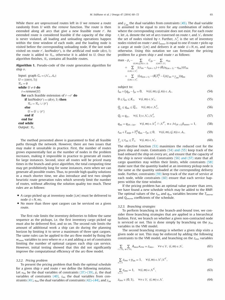

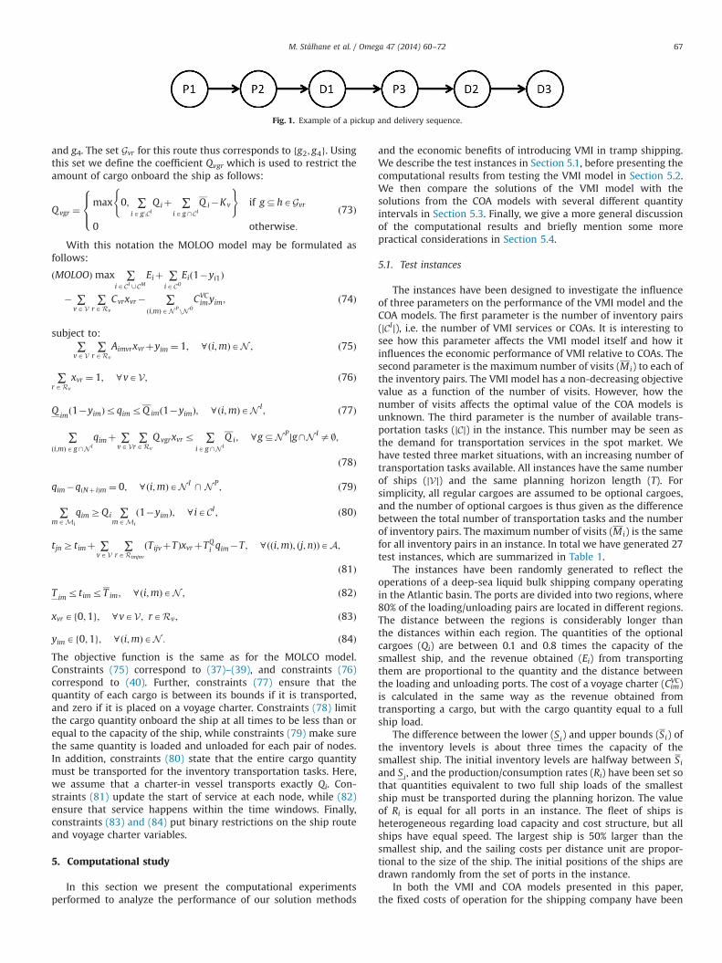
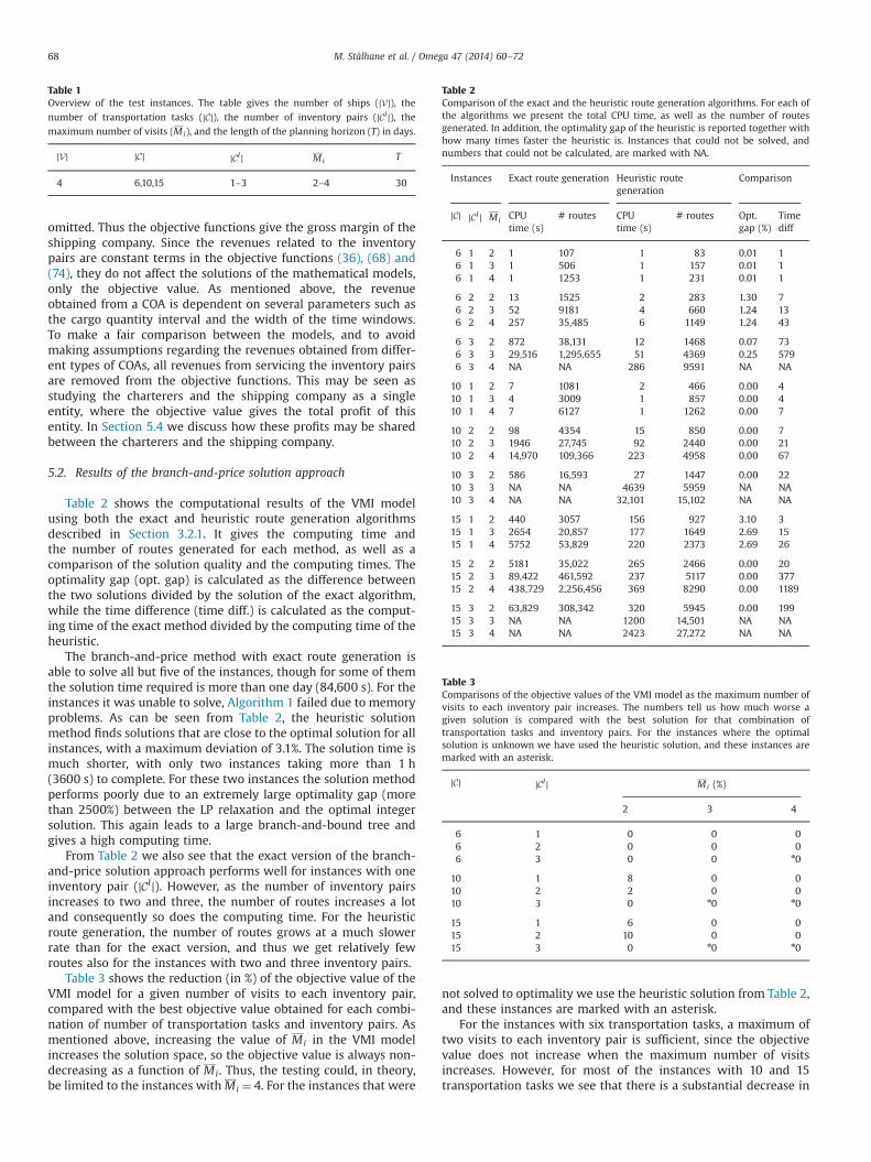


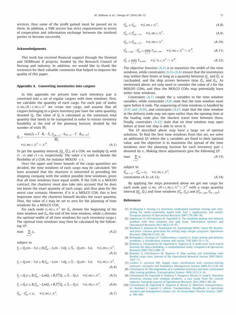


![[Music Score] Big Band - The Lady is a Tramp](https://static.documents.pub/doc/80x56/544cec46b1af9f6c0c8b4662/music-score-big-band-the-lady-is-a-tramp.jpg)


