NASA
Technical
Paper3349
1993
Verification ofFault-Tolerant Clock
Synchronization Systems
Paul S. Miner
Langley Research Center
Hampton, Virginia
National Aeronautics andSpace Administration
Office of Management
Scientific and TechnicalInformation Program
https://ntrs.nasa.gov/search.jsp?R=19940012976 2018-07-16T05:24:58+00:00Z
Contents
List of Tables................................. V
List of Figures ................................ v
Smnmary ' ................................. vi
Chapter 1 Introduction ............................ 1
Chapter 2 Clock Definitions .......................... 4
2.1 Notation ................................ 4
2.2 Conditions ............................... 8
2.2.1 Properties of Convergence Function ................. 82.2.2 Physical Properties ....................... 11
2.2.3 Interval Constraints 13
2.2.4 Constraints oil Skew 142.2.5 Umlecessary Conditions ..................... 15
Chapter 3 General Solution for Bounded Delay ................ 17
3.1 Bounded Delay Offset 18
3.2 Bounded Delay for Two-Algorithm Schemata ............... 21
3.3 EHDM Proofs of Bounded Delay ..................... 22
3.4 New Theory Obligations ........................ 24
Chapter 4 Fault-Tolerant Midpoint as an Instance of Schneider's Schelna ..... 26
4.1 Translation Invariance 27
4.2 Precision Enhancement 27
4.3 Accuracy Preservation 30
4.4 EtII)M Proofs of Convergence Properties ................. 30
Chapter 5 Design of Clock Synchronization System .............. 32
5.1 Description of Design ......................... 32
5.2 Theory Obligations .......................... 35
Chapter 6 Initialization and Transient Recovery . ............... 37
6.1 Initial Synchronization 38
6.1.1 Mechanisms for Initialization ................... 396.1.2 Comparison With Other Approaches ................ 45
.ooIll
PI_CIIIi:)_6i PAGE BLANK NOT FILMtE.D
456.2 Transient Reccvery .........................
6.2.1 Theory Ccnsiderations ...................... 456.2.2 Satisfy rpred ......................... 47
6.2.3 Comparison With Other Approaches ................ 47
Chapter 7 Concluding Remarks ....................... 48
Appendix A -PIoof cf Agreement ....................... 50
Appendix B--Bounded Delay Modules ..................... 61
Appendix C--Fault-Tolerant Midpoint Modules ................. 98
Appendix D--Utility Modules ........................ 114
135References ........................... : .....
iv
List of Tables
2.1 Clock Notation .............................. 9
2.2 Constants ................................ 9
List of Figures
2.1 Four-clock system ............................. 5
2.2 Determining VCp(t) ............................ 7
5.1 Informal block model of clock synchronization circuit ............ 34
6.1 Key parts of synchronization interval ................... 38
6.2 Pathological scenario--assumed perfection ................. 40
6.3 End of interval initialization ....................... 41
6.4 Pathological end of interval initialization .................. 42
W.5 End of interval initialization-- time-out .................. 42
6.6 End of interval initialization: d faulty benign ............... 44
6.7 End of interval initialization: d faulty- malicious .............. 44
V
Summary
A critical function in a fault-tolerant computer architecture is tile synchronization of
the redundant computing elements. One means of accomplishing this is for each com-
puting element to maintain a local clock that is periodically synchronized with the other
clocks in the system. The synchronization algorithm must include safeguards to ensure
that failed components do not corrupt the behavior of good clocks. Reasoning about fault-
tolerant clock synchronization is difficult because of the possibility of subtle interactions
involving failed components. Therefore, mechanical proof systems are used to ensure that
the verification of the synchronization system is correct.
In 1987, Schneider (Tech. Rep. 87-859, Cornell Univ.) presented a general proof
of correctness for several fault-tolerant clock synchronization algorithms. Subsequently,
Shankar (NASA CR-4386) verified Schneider's proof by using the mechanical proof sys-
tem EHDM. This proof ensures that any system satisfying its underlying assumptions will
provide Byzantine fault-tolerant clock synchronization. This paper explores the utility of
Shankar's mechanization of Schneider's theory for the verification of clock synchronization
systems.
In tile course of this work, some limitations of Shankar's mechanically verified the-
ory were encountered. These limitations include one assumption that is to() strong and
also insufficient support for reasoning about recovery from transient faults. With minor
modifications to the other assumptions, a mechanically checked proof is provided that
eliminates the overly strong assumption. In addition, the revised theory allows for proven
recovery from transient faults.
Use of tim revised theory is then illustrated with the verification of an abstract design
of a fault-tolerant clock synchronization system. The fault-tolerant midpoint convergence
function is proven with EHDM to satisfy the requirements of the theory. Then a design
using this convergence function is shown to satisfy the remaining constraints.
vi
Chapter 1
Introduction
At first glance, the development of fault-tolerant computer architectures does not. ap-
pear to be a difficult problem. Clearly, three computers shouhi be sufficient to survive a
single fault. A simple majority vote should mask any errors caused by a failed compo-
nent. However, to determine when to vote, tile computers must be synchronized. This
synchronization is easy with a perfect clock that coordinates actions among the re(tundant
computing elements. Unfortunately, clocks also fail. Thus, each redundant computing el-
ement nmst inaintain its own clock. No clock keeps perfect time; all drift, with respect to
some reference standard time. Sinfilarly, clocks drift with respect to each other. Therefore,
regular synchronization of the clocks of the redundant computing elements is necessaryl
An obvious algorithm for synchronizing clocks of three computers is for each to periodi-
cally read the clocks of the other two and then set; its own clock to equal the mid value
of the three observed values. Intuitively, this algorithm should work, but consider what.
happens if one clock fails so that it behaves in an arbitrary fashion. The classic example
is given by Lamport and Melliar-Smith (ref. 1). Suppose that the clock for computer A
shows 1:00, the clock for computer B shows 2:00, and tile clock for computer C has failed
in such a way that when A reads C's clock it shows 0:00 and when B reads C's clock it.
shows 3:00. Clearly, neither A nor B has a compelling reason to adjust its clock and they
nmy continue to drift apart. The presentation of Lamport and Melliar-Smith contimms
with a formal statement of the clock synchronization problem and presents three verified
solutions. Subsequently, a number of other solutions to problems related to clock syn-
chronization were developed, including those in references 2 through 7. A survey of the
various approaches is given by Ramanathan, Shin, and Butler (ref. 8).
Schneider (ref. 9) recognized that the many approaches to clock synchronization can
be presented as refinements of a single, verified paradigm. Shankar (ref. 10) provides
a mechanical proof (using EHDM (ref. 11)) that Schneider's schema achieves Byzantine
fault-tolerant clock synchronization, provided that 11 constraints are satisfied. (A failure
that exhibits arbitrary or malicious behavior is called a Byzantine fault, in reference to the
Byzantine Generals problem of Lamport, Shostak, and Pease (ref. 12).) One goal of this
paper is to examine the utility of Shankar's mechanically checked version of Schneider's
theory in the verification of a particular clock synchronization system.
The field of fault-tolerantcomputingis repletewith examplesof intuitively correctapproachesthat werelater shownto beinsufficient.In onesystem,thedesignofthe fault-tolerancemechanismwascitedasa major contributorto the unreliabilityof the system(ref. 13). Becauseof the extremelevelof reliability requiredfor manyfault-tolerantsys-tems,employingrigorousverificationtechniquesis necessary.(An oftenquotedrequire-ment for critical systemsemployedfor civil air transportis a probabilityof catastrophicfailure lessthan 10-9 for a 10-hourflight (ref. 14).)Onesuchtechniqueis the useof for-malproofto establishthat a designhascertainproperties.Additionalcertaintyis gainedby confirmingthe verificationwith a mechanicalproofsystem,suchas EHDM.Anotherbenefitof machine-checkedproofsis that the underlyingassumptionsaremadeexplicit tohelpto clearlydefinethe necessaryverificationconditions.
Shankar'sverificationof Schneider'sprotocolprovidesa trustedformalspecificationof a clocksynchronizationsystem.Manyof the difficult aspectsof the proofhavebeenverifiedin a genericmanner;all that is requiredto verify a synchronizationsystemis todemonstratethat it meetsthe requirementsof the generaltheory. This paperis a resultof the first attempt to verify a designusingShankar'smachine-checkedtheory (ref. 10).In the courseof the verification,somedifficultieswereencounteredwith the underlyingassumptions.The mostsignificantproblemwasthat oneof the assumptions,boundeddelay,wastoo strong. Boundeddelayassertsthat thereis a boundon theelapsedtimebetweensynchronizationeventsonanytwogoodclocks.Forsomeprotocols,thispropertyis the keyrequiredto maintainsynchronization.The proofof boundeddelaycanbe asdifficult as the generalsynchronizationproperty. This paperrevisesShankar'sgeneraltheorybymodifyingtheremainingconstraintsto enablea generalproofof boundeddelay.
In an effort to demonstratethe applicabilityof formalproof techniquesto the ver-ificationof highly reliablesystems,the LangleyResearchCenteris currentlyinvolvedinthe developmentof a formallyverifiedReliableComputingPlatform(RCP)for real-timedigital flight control(refs.15,16,and17).Thefault-tolerantclocksynchronizationcircuitis intendedto be part of a verifiedhardwarebasefor the RCP.The primary intent ofthe RCP is to providea verifiedfault-tolerantsystemthat is provento recoverfrom aboundednumberof transientfaults. The currentmodelof the systemassumes(amongotherthings)that the clocksaresynchronizedwithin aboundedskew(ref. 16). Theclocksynchronizationcircuitry alsoshouldbeableto recoverfrom transientfaults. Originally,the interactiveconvergencealgorithm(ICA) of Lamport and Melliar-Smith(ref. 1) wasto be the basisfor the clocksynchronizationsystem,the primary reasonbeingthe exis-tenceof a mechanicalproofthat thealgorithmiscorrect(ref. 18).However,modificationsto ICA to' achievetransient-faultrecoveryarecomplicated.The fault-tolerantmidpointalgorithmof WelchandLynch(ref. 2) is morereadilyadaptedto transientrecovery.
Even though the clocksynchronizationcircuit wasdesignedto recoverfrom tran-sientfaults,therewasnosupportin themachine-checkedtheoryfor provenrecoveryfromsuchfailures.Whenthe machine-checkedtheorywasrevisedto removetheassumptionofboundeddelay,additionalmodificationsweremadeto expandthetheoryto accommodateprovenrecoveryfrom a boundednumberof transientfaults.
The synchronizationcircuit is designedto toleratearbitrarily maliciouspermanent,intermittent,and transienthardwarefaults. A fault is definedasa physicalperturbationalteringthefunctionimplementedby aphysicaldevice.Intermittentfaultsarepermanentphysicaldefectsthat donot continuouslyalterthe functionof a device(e.g.,a loosewire).A transientfault iscausedby aone-shot,short-durationphysicalperturbationof a device(e.g.,a cosmicray or electromagneticeffect). Thisperturbationcanresult in anyof thefollowingsituations:
1. Permanentdamageto thedevice
2. Nodamagewith a persistenterror induced
3. Nodamagewith the systemrecoveringfromtheerroneousstate
The first situation is classifiedmsa permanentfault; tile secondand third are transientfaults. A gooddesigncaneliminatethe secondsituationby establishinga recoverypathfromall possiblesystemstates.Sucha designiscalledself-stabilizing(ref. 19). Oncethephysicalsourceof the fault is removed,the devicecan flmctioncorrectly.The synchro-nizationcircuit is designedto automaticallyrecoverfroma boundednumberof transientfailures.
Most proofsof fault-tolerantclocksynchronizationalgorithmsareby induction onthe numberof synchronizationintervals.Usually,the basecaseof the induction,the ini-tial skew,is assumed.The descriptionsin references1, 9, 19,and 18all assumeinitialsynchronizationwith nomentionof howit is achieved.Others,includingreferences2, 4,6, and 20,addressthe issueof initial synchronizationand givedescriptionsof how it isachievedin varyingdegreesof detail. In provingan implementationcorrect,the detailsof initial synchronizationcannotbeignored.If the initializationschemeis robustenough,it canalsoserveasa recoverymechanismfrom multiplecorrelatedtransientfailures(asnotedin ref. 20).
The chaptersin this paperarearrangedby decreasinggenerality. The most gen-eralresultsarepresentedfirst andareapplicableto a numberof designs.The useof thetheory is then illustratedby applicationto a specificdesign. In Chapter2, the defini-tionsandconstraintsrequiredby thegeneralclocksynchronizationtheoryarepresented.Chapter3 presentsthe main revisionmadeto Shankar'stheory,which is removingtheassumptionof boundeddelay. Chapter4 presentsmechanicallycheckedproofsthat thefault-tolerantmidpointconvergencefunctionsatisfiestheconstraintsrequiredby the the-ory. In Chapter5, a hardwarerealizationof a fault-tolerantclocksynchronizationcircuitis introducedand shownto satisfythe remainingconstraintsof the theory. Finally insection6, the mechanismsfor achievinginitial synchronizationandtransientrecoveryarepresented.Modificationsto the theory to supportthe transientrecoveryargumentsarealsopresented.
The informationpresentedin this report wasincludedin a thesisofferedin partialfulfillmentoftherequirementsfor theDegreeof Masterof Science,TheCollegeof Williamand Mary in Virginia,Williamsburg,Virginia, 1992.
Chapter 2
Clock Definitions
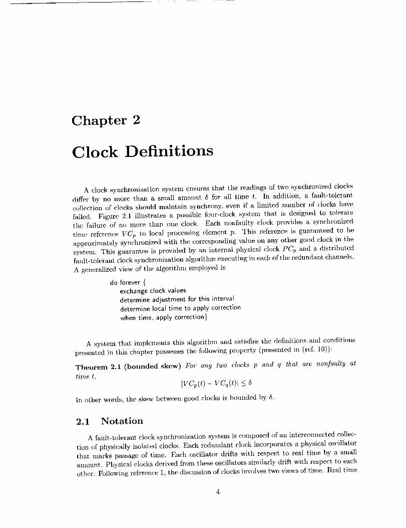
A clock synchronization system ensures that the readings of two synchronized clocks
differ by no more than a small amount 5 for all time t. In addition, a fault-tolerant
collection of clocks should maintain synchrony, even if a limited number of clocks have
failed. Figure 2.1 illustrates a possible four-clock system that is designed to tolerate
the failure of no more than one clock. Each nonfaulty clock provides a synchronized
time reference VCB to local processing clement p. This reference is guaranteed to be
approximately synchronized with the corresponding value on any other good clock in the
system. This guarantee is provided by an internal physical clock PCp and a distributed
fault-tolerant clock synchronization algorithm executing in each of the redundant channels.
A generalized view of the algorithm employed is
do forever {
exchange clock values
determine adjustment for this interval
determine local time to apply correction
when time, apply correction}
A system that implements this algorithm and satisfies the definitions and conditions
presented in this chapter possesses the following property (presented in (ref. 10)):
Theorem 2.1 (bounded skew) For any two clocks p and q that are nonfaulty at
time t,Ivcp(t) - vcq(t)l <
In other words, the skew between good clocks is bounded by 5.
2.1 Notation
A fault-tolerant clock synchronization system is composed of an interconnected collec-
tion of physically isolated clocks. Each redundant clock incorporates a physical oscillator
that marks passage of time. Each oscillator drifts with respect to real time by a small
amount. Physical clocks derived from these oscillators similarly drift with respect to each
other. Following reference 1, tile discussion of clocks involves two views of time. Real time
I VCa I VCb
algorithm ]_ I algorithm
Figure 2.1: Four-clock system.
corresponds to an assunmd Newtonian time frame; clock time is the measurement of this
time frame by some clock. Identifiers representing real-time quantities will be denoted by
lower case letters, e.g., t, s: Var time. Here, t and s are variables (in tile logical theory) of
type time. A declaration without the keyword Var defines a constant, e.g., tl: time defines
the constant tl of type time. Typically, time is taken as ranging over the real numbers.
Clock time will be represented by upper case letters, e.g., T, S: Var Clocktime. Although
Clocktime is often treated as ranging over tile reals (refs. 2, 10, and 18), a physical realiza-
tion of a clock marks time in discrete intervals. In this presentation Clocktime is assumed
to range over tile integers. Tile unit for both time and Clocktime is the tick. There are
two sets of functions associated with the physical clocksl: functions mapping real time toclock time for each process p,2
PCp : time --_ Clocktime
and functions mapping clock time to real time,
pc v : Clocktime -_ time
]Shankar's presentation inchMes only the mappings from time t<>Clocktime. The mappings from Clock-time to time arc added here because they are more natural reprcsenlations for some of the proofs.
:Declarations of the form f : (_ --, ,_ define a function f with domain o and range 3.
The notation PCp(t) represents the reading of p's physical clock at real time t, and pcp(T)denotes the earliest real time that p's clock reads T. By definition, PCp(pcp(T)) = T for
all T. In addition, we assume that pcp(PCp(t)) <_ t < pcp(PCp(t) + 1).
The purpose of a clock synchronization algorithm is to make periodic adjustments to
local clocks to keep a distributed collection of clocks within a bounded skew of each other.
This periodic adjustment makes analysis difficult; therefore an interval clock abstractionis used in the proofs. Each process p has an infinite number of interval clocks associated
with it, each of these is indexed by the number of intervals since the beginning of the
protocol. An interval corresponds to the elapsed time between adjustments to the virtualclock. These interval clocks are equivalent to adding an offset to the physical clock of a
process. As with the physical clocks, they are characterized by two functions: ICp : time --_
Clocktime and iCip : Clocktime --, time. If we let adj; : Clocktime denote the cumulative
adjustment made to a clock as of the ith interval, we get the following definitions for the
ith interval clock:
IC*p(t) = PCp(t) + adj;
icp(T) = pcp(T- adjp)
From these definitions, it is simple to show ICp(iCip(T) ) = PCp(pcp(T - adjp) ) + adjip = T
for all T. Sometimes it is more useful to refer to the incremental adjustment made in a
particular interval than to use a cumulative adjustment. By letting ADJ_ = adjp +1 - adjp,
we get the following equations relating successive interval clocks:
IC_+l(t) = ICp(t) + APJp
ic;+l(T) = ic;(T- ADJp)
A virtual clock, VCp : time _ Clocktime, is defined in terms of the interval clocks by the
equationvcp(t) = Ic;(t) (t; < t < t;
i denotes the instant in real time that process p begins the ith interval clock.The symbol tpNotice that there is no mapping from Clocktime to time for the virtual clock because VCp
is not necessarily monotonic; the inverse relation might not be a function for some syn-
chronization protocols. The definition of VCp(t) from the equations for IC is illustrated
in figure 2.2.
Synchronization protocols provide a mechanism for processes to read each other'sclocks. The adjustment is computed as a function of these readings. In Shankar's presen-
tation, the readings of remote clocks are captured in function Op+1 : process --* Clocktime,
where _)_+a(q) denotes process p's estimate of q's ith interval clock at real time t_+_
ICq(tp )). Each process executes the same (higher order) convergence function,(i.e., _ i+1cfn : (process, (process _ CIocktime)) _ CIocktime, to determine the proper correction to
apply. 3 Shankar defines the cumulative adjustment in terms of the convergence function
as follows:
aThe domain of a higher order function can include functions. In this case, the second argument of cfn
is itself a function with domain process and range C[ocktime.
vc (t)pc (t)
I_/ -_p (t)
Ai"
Figure 2.2: Determining VCp(t). Scale does not permit display of ICp as step function.
adj;+' = cY (v,O;+') - Pep(t;+')
adj°p = 0
The following can be simply derived from the preceding definitions:
Pep(t; +1) -= IC_+l(tip +1) = cfrt(p, O; +1)
ICp+l(t) = cfn(p, O; +1) q- PCp(t) - PCp(tp +')
ADair = cfn(p,O; +1 ) i i+1- ICv(t v )
Using some of these equations and the conditions presented in section 2.2, Shankar mechan-
ically verified Schneider's paradigm. Chapter 3 presents a general argument for satisfying
one of the assumptions of Shankar's proof. The argument requires some modifications
to Shankar's constraints and introduces a few new assumptions; in addition, some of the
existing constraints are rendered unnecessary.
A new constant, R : Clocktime, is introduced which denotes the expected duration
of a synchronization interval as measured by clock time. (That is, in the absence of drift
and jitter, no correction is necessary for the clocks to remain synchronized. In this ease,
the duration of an interval is exactly R ticks.) We also introduce a collection of distin-
guished clock times S i : Clocktime, such that S i = iR + S ° and S o is a particular clock
i definedtime in the first synchronization interval. We also introduce the abbreviation sp
as equal to icp(Si). The only constraints on S i are that, for each nonfaulty clock p and
real times tl and t2,
(vcp(tl) = s _) A (vc_(t2) = s _) D tl = t2
and some real time t exists, such that
vc_(t) = s _
The rationale for these constraints is that we want to unambiguously define a clock time
in each synchronization interval to simplify the arguments necessary to bound separation
of good clocks. If we choose a clock time near the instant that an adjustment is applied,
it is possible that the VC will never read that value because the clock has been adjusted
ahead or that the value will be reached twice because of the clock being adjusted back. In
reference 2, the chosen unambiguous event is the clock time that each good processor uses
to initiate the exchange of clock values. For other algorithms, any clock time sufficiently
removed from the time of the adjustment will suffice. A simple way to satisfy these
constraints is to ensure that for all i,
Avs; < r;' < s"' - Avs;
where T; +1 = ICp(tip+l).
Table 2.1 summarizes tile notation for the key elements required for a verified clock syn-
chronization algorithm. Table 2.2 presents the many constants used in section 2.2. They
are described when they are introduced in the text but are included here as a convenient
reference.
2.2 Conditions
This section presents the assumptions required in the proof of theorem 2.1. The
conditions can be separated into three main classes: abstract properties required of the
convergence function, physical properties of the system, and various constraints on the
length of the synchronization interval. Additional constraints are also determined by the
proof of theorem 2.1. Some of these properties are taken directly from Shankar's presenta-
tion, whereas others are revised in order to facilitate verification of a clock synchronization
system. Additional modifications are made to enable proofs of transient-fault recovery.
2.2.1 Properties of Convergence Function
Synchronization algorithms use a convergence function cfn(p, O) to determine the ad-
justment required to maintain synchrony. The general theory requires that the conver-
gence function satisfy three properties: translation invariance, precision enhancement,
and accuracy preservation. Shankar mechanically proves that the interactive convergence
function of Lamport and Melliar-Smith (ref. 1) satisfies these three conditions. A mechan-
ically checked proof that the fault-tolerant midpoint function used by Welch and Lynch
(ref. 2) satisfies these conditions is presented in Chapter 4 and was previously reported
Table2.1: ClockNotation
Notation DefinitionPep(t)p.p(T)
ic;(r)VCp(t)
T o
'T'; +1
t iP
R
S o
Si
i8p
adj;
ADJ_
0_+ 1
4n(v, e;+')
Reading of p's physical clock at real time t
Earliest real time that p's physical clock reads T
Reading of p's ith interval (:lock at real time t
Earliest real time that p's ith interval clock reads T
Reading of p's virtual clock at time t
CIocktime at beginning of protocol (for all good clocks)
CIocktime for VCp to switch fr(ml ith to (i + 1)th interval clock
Real time that, processor p begins ith synchronization
interval (tp +l = ic i (Tj +l))" p_p
CMcktime duration of synchronization interval
Special CIocktime in initial interval
Unambiguous clock time in interval i; S i = iR + S °
Abbreviation for icip( S i)
iCumulative adjustment to p's physical clock up through tp
Abbreviation for adj_ +1 - adj])
Array of clock readings (local to p) such that, (-)_,(q) is p's
reading of q's ith interval clock at, t_ +1
Convergence flmction executed by p to establish VCp(@ *1 )
Table 2.2: Constants
Constant Definition
8s : Clocktime
: CIocktime
p : number
J : time
_3 : time
,L_read : time
rmiT _ : time
rma.: time
A : Clocktime
A': number
c_(_3' + 2A') : number
Bound on skew at beginning of protocol
Bound on skew for all time
Allowable drift rate for a good clock, 0 _< p << 1
,i to a (p and q working)Maximum elapsed time from ,_p ,Sq
i i working)Maxinmm ela,t)sed time from tp to tq (p and q
,i and ,i for p toMaximum separation t)etwecn ,sp ,Sq,
accurately read q, /t' <_ /'_l_,,_d< 1?/2
i tit+.lMinimum elapsed time from tp to for good p
i_1 for goodpMaximuul elat)sed time from t_, to tp
Bound on error reading a remote clock
Reformulated error bound for reading a reinote clock
Bound on ADJ_ for good p and all i
in reference 21. Schneider presents proofs that a number of other protocols satisfy these
properties in reference 9. The conditions in this section are unchanged from Shankar's
presentation.
The constraints on the convergence function assume a bound on the number of faults
to be tolerated. This condition is stated here as condition 1; in Shankar's presentation,
this was condition 8.
Condition 1 (bounded faults) At any time t, the number of faulty processes is at
most F.
Translation invariance means that the value obtained by adding X : Clocktime to the
result of the convergence function should be the same as adding X to each of the clock
readings used in evaluating the convergence function. This was condition 9 in Shankar's
presentation. The statement of this condition adapts notation from the lambda calculus.
The symbol _ is used to define an unnamed function. For example, ._x.x + 2 defines a
function of one argument x that returns the sum of x and 2. For a detailed treatment of
the lambda calculus, see reference 22.
Condition 2 (translation invariance) For any function 0 mapping clocks to clock
values,efn(p, (An: O(n) + X)) = cfn(p, O) + X
Precision enhancement is a formalization of the concept that, after executing the con-
vergence function, the values of interest should be close together. Essentially, if the argu-
ments presented to the convergence function are sufficiently similar, there is a bound on
the difference of the results. In the proof of theorem 2.1, this condition ensures that if a
large enough collection of good clocks is synchronized in one interval, then they will still
be synchronized in the next. This was Shankar's condition 10.
Condition 3 (precision enhancement) Given any subset C of the N clocks with
ICI > N - F and clocks p and q in C, then for any readings 7 and 0 satisfying the
conditions
1. For any l in C, b(e) - 0(e)l <_ x
2. For any l, m in C, I'T([) - "_(m)l <- Y
s. Forany l, in C, 10(e)- <_Y
there is a bound rr(X, Y) such that
Icfn(p,_/) - cfn(q,O)l < rr(X, Y)
10
Accuracy preservation formalizes the notion that there should be a bound on the amount of
correction applied in any synchronization interval. Accuracy preservation was condition 11in Shankar's report.
Condition 4 (accuracy preservation) Given any subset C of the N clocks with
ICI > N- F and clock readings 0 such that, for any l and m in C, the bound
[0(_) - O(m)l <_ X holds, there is a bound or(X) such that for any p and q in C,
Icfn(p,o) - O(q)l_<
For some convergence flmctions, the properties of precision enhancement and accuracy
preservation can be weakened to simplify arguments for recovery from transient faults.
Precision enhancement can be satisfied by many convergence functions even if p and q are
not in C. Similarly, accuracy preservation can often be satisfied even when p is not in C.
2.2.2 Physical Properties
Some of the conditions characterize the expected physical properties of the system.
We rely on experimentation and engineering analysis to demonstrate these conditions.
The rate at which a good clock can drift from real time is bounded by a small positiveconstant p. Typically, p < 10 -5.
Condition 5 (bounded drift) There is a nonnegative constant p such that if p's
clock is nonfaulty during the interval from T to S(S > T), then
S-T
l+p-- _<pep(S) - _<(1+ .)(S - T)
This condition replaces Shankar's condition 2. This assumption is stronger than Shankar's
bound on drift, but the change is necessary to accommodate the integer representation of
Clocktime. However, if the unit of time is taken to be a tick of Clocktime and Clocktime
ranges over the integers, we can then derive the following bound on drift, which is sufficient
for preserving Shankar's mechanical proof (with minor modifications):
Corollary 5.1 If p's clock is not faulty during the interval from t to s then,
[(s - t)/(1 + p)j < PCp(s) - PCp(t) < [(1 + p)(s - t)l
Note that with Shankar's algebraic relations defining various components of clocks, we
can use these constraints to bound the drift of any interval clock (iCp) for any i.
The following corollary to bounded drift limits the amount two good clocks can driftwith respect to each other during the interval from T to S.
11
Corollary 5.2 If clocks p and q are not faulty during the interval from T to S,
[pCp(S) - pCq(S)l <_ IpCp(T) - pcq(T)l + 2p(S - T)
This corollary is used in bounding the amount of skew caused by drift during each syn-
chronization interval.
We can also derive an additional corollary (adapted from lemma 2 of ref. 2).
Corollary 5.3 If clock p is not faulty during the interval from T to S,
L(pcp(S) - S) - (pep(T) - T)I <_ plS - TI
This corollary recasts bounded drift into a form more useful for some proofs. A similar
relation holds for PC.
All clock synchronization protocols require each process to obtain an estimate of the
clock values for other processes within the system. The determination of this estimate is
called reading the remote clock, even if there is no direct means to observe its value. Typi-
cally, some underlying communication protocol is employed which allows a fairly accurate
estimate of other clocks in the system. Error in this estimate can be bounded but not
eliminated. A discussion of different mechanisms for reading remote clocks can be found
in Schneider (ref. 9). Shankar's statement of the bound on reading error is as follows:
Shankar's Condition 7 (reading error) For nonfaulty clocks p and q,
i i+1 Op÷l(q)l < A[ICq(tp )-
This condition neglects an important point. In some protocols, the ability to accurately
read another processor's clock is dependent on the clocks being already sufficiently syn- ichronized. Therefore, we add a precondition stating that the real-time separation of Sp
i is bounded by some value of flread. The precise value of _r,.',_ required to en-and Sqsure bounds on the reading error is determined by the implementation, but in all cases
fl_ _< firead < R/2. Another useful observation is that an estimate of the value of a remote
clock is subject to two interpretations. It can be used to approximate the difference in
Clocktime that two clocks show at an instant of real time, or it can be used to approximate
the separation in real time that two clocks show the same Clocktime.
Condition 6 (reading error) For nonfaulty clocks p and q, if ISp - Sql <_ _read,
ICp(tp ))l < A1. i i+1)--O;+1 i+1 rC,(ti+,))_(iCq(t_p+l)_ i i+,IICq(tp (q)l = I(Op (q)- ---p,-p
(_cp(Tp )- ))1 A- ICp(tp ))-2. I(Op+'(q) _ i+1 -i i+, icq(T_;+' <
-- ICp(tp )) - -3. I(O_+l(q) _ _+1 _ (idp(Si) ieq(Si))l < A'
12
Thefirst clausejust restatesthe existingreaderror conditionto illustrate that the readerror canalsobeviewedasthe errorin anestimateof thedifferencein readingsof Clock-time,that is,theestimateallowsusto determineapproximatelyanotherclock's reading at
a particular instant of time. The second clause recognizes that this difference can also be
used to obtain an estimate of tire time when a remote clock shows a particular Clocktime.
For these relations, elements of type Clocktime and time are both treated as being of type
number. Clocktime is a synonym for integer, which is a subtype of number, and time is a
synonym for number. The third clause is tire one used in this paper; it reiates real-time
separation of clocks when they read oci to tile estimated difference when the correction
is applied. A bound on this could be derived from the second clause, but it is likely
that a tighter bound can be derived from the implementation. Since the guaranteed skew
is derived, ill part, from the read error, we wish this bound to be as tight as possible.
For this reason, we add it as an assumption to be satisfied in the context of a particularimplementation.
2.2.3 Interval Constraints
The conditions constraining the length of a synchronization interval are determined,
in part, by the closeness of tile initial synchronization. The following condition replacesShankar's condition 1:
Condition 7 (bounded delay init) For nonfaulty processes p and q,
It';- <_ - 2p(S° - T°)
A constraint similar to Shankar's can be easily derived from this new condition by us-
ing the constraint on clock drift. (Shankar's condition 1 is an immediate consequence of
lemma 2.1.1 in appendix A.) An immediate consequence of this and condition 5 is that
14- _<J.
Shankar assumes a bound on the duration of tile synchronization interval.
Shankar's Condition 3 (bounded interval) For nonfaulty clock p,
0 < r,,,,_ _< t;+1 i <-- _,p __ 'FT_uta:
The terms r,m_ and r,,,,** are uninstantiated constants. In this formulation, a nominal
duration (R) of an interval is assumed determined from the implementation. We set a
lower bound on R by placing restrictions on the events S i. This restriction is done by
bounding the amount of adjustment that a nonfaulty process can apply in any synchro-
nization interval. In Chapter 3, the term ct(,q' + 2A') is shown to bound [AD,Ipl fornonfaulty process p. The function _ is introduced in condition 4, /)' is a bound on the
separation of clocks at a particular Clocktime in each interval, and A' bounds tile error inestimating the value of a remote clock.
13
Condition 8 (bounded interval) For nonfaulty clock p,
S i + _(_' + 25') < T_ +1 < S i+1 - _(3' + 25')
By remembering that S i = iR + S °, it is easy to see that R > 2_(_' + 2A'). Clearly, we
can define rmin as (R - c_(_' + 2A'))/(1 + p) and r,,_,_ as (1 + p)(R + _(_' + 25')).
We need a condition to ensure that process q does not start its (i + 1)th clock before
process p starts its ith clock. The following condition is sufficient to meet this requirement,
which is a simple restatement of Shankar's condition 6, using the definition of r,ni_ from
Shankar's condition 3.
Condition 9 (nonoverlap)
_<R - (_(/_' + 2A')
l+p
This condition essentially defines an additional constraint on R; namely, that R >_i and i
(1 + p)/3 + c_(/3' + 2A'), when/3 bounds the maximum separation of tp tq.
2.2.4 Constraints on Skew
Shankar assumes the following additional conditions for an algorithm to be verified in
this theory. These additional constraints were determined in the course of his proof of
theorem 2.1.
1. ?r(2A + 2/3p, (ss + 2p(rm_z + 13) + 2A) <_ 6s
2. 6S + 2prma, <_ 6
3. _((ss + 2p(rm,, +/_) + 2A) + A + p_ <_ (5
These conditions relate the skew (5 guaranteed by the theory with the properties of preci-
sion enhancement and accuracy preservation.
When Clocktime was changed to range over the integers, these conditions had to be
modified. The bounds were altered to correspond to the revised version of bounded drift.
Shankar's version of bounded drift was converted to correspond to corollary 5.1. (This
is stated as axioms rate_l and rate_2 in module clockassumptions (appendix A).) The
mechanical proof was rerun and yielded the following constraints:
1. _-(/2A + 2/3p_ + 1,(58 + [2p(rmax+Z) +2A] + 1) < 6s
2. (ss + [2prm_ + 1 <_ (5
3. o_((ss + [2p(rmax + _) + 2A] + 1) + 5 + [2p/3] + 1 < (5
14
Theargumentsusedareidenticalto thosepresentedby Shankar.Theonly differenceisthat additionalmanipulationswereneededwith the floor andceilingfunctionsin orderto completetheproof.AppendixA containsthe proofchainanalysiswhichconfirmsthattheseconstraintsaresufficientto provetheorem2.1.
Since p is typically very small (< 10-5), the above reworked constraints appear overly
conservative. It is possible to prove theorem 2.1 by assuming the following:
1. 4pr,,oj:+ 7r(L2A'+ 2j, L_' + 2A'J) <#3'
2. [(1 + + 2pr,,,ox] _<
3. c_([/Y + 2A'J) + A + I2p/3] + 1 _< (5
A proof sketch can be found in appendix A.
2.2.5 Unnecessary Conditions
Two of the conditions presented in Shankar's report were found to be unnecessary.
Shankar and Schneider both assume tile following conditions in their proofs:
Shankar's Condition 4 (bounded delay) For nonfaulty clocks p and q,
The condition states that the elapsed time between two processes starting their ith in-
terval clock is bounded. This property is closely related to the end result of the general
theory (bounded skew) and should be derived in the context of an arbitrary algorithm.
The related property for nonfaulty clocks p and q,
1.2;- 41-< z'
is proven independently of the algorithm in Chapter 3. This gives sufficient information
to prove bounded delay directly from the algorithm; however, this proof depends on the
interpretation of T¢ +1. Two interpretations and their corresponding proofs are also givenin Chapter 3.
The next condition states that all good clocks begin executing the protocol at the
same instant of real time (and defines that time to be 0):
Shankar's Condition 5 (initial synchronization) For nonfaulty clock p,
0= 0tp
It is not possible to guarantee that all clocks start at the same instance of time; thus,
no implementation can guarantee this property. This property is used, in conjunction
with Shankar's condition 1, to ensure the base case of the induction required to prove
15
theorem2.1. By definingtop = iC°p(T°), we can readily prove tile base case with condi-
tions 5 and 7. Some constant clock time known to all good clocks is represented by T °0 states that all nonfaulty
(i.e., T O is the clock time in the initial state). The definition of tp
clocks start tile protocol at the same CIocktirne.
16
Chapter 3
General Solution for Bounded
Delay
The condition of bounded delay asserts that any two nonfaulty clocks begin each syn-
chronization interval at approximately tile same real time. This property is nearly as
strong as theorem 2.1. In fact, the result follows immediately for some synchronization
protocols. This chapter establishes, for many synchronization protocols, that the condi-
tion of bounded delay follows from the remaining conditions enunlerated in Chapter 2.
Schneider's schema assumes that
- tq[ _ /3
i denotes tile real time that clock p begins its ith intervalfor good clocks p and q, where tp
clock (this is condition 4 in Shankar's presentation). Anyone wishing to use the general-
ized proof to verify the correctness of an implementation must prove that this property
is satisfied by their implementation. For the algorithnl presented in reference 2, this is anontrivial proof.
The difficulty stems, in part, from the inherent ambiguity in the interpretation of t_,+1Relating the event to a particular clock time is difficult because it serves as a crossover
point between two interval clocks. The logical clock implemented by the algorithm
undergoes an instantaneous shift in its representation of time. Thus the local clock read-
ings surrounding the time of adjustment may show a particular clock time twice or never.
Tile event tp+1 is determined by the algorithm to occur when ICv(t) = Tp+l; that is Tp _1
is the clock time for applying the adjustment ADJ; (adj_ +l .i= - adjp). This also meansthat tp+i = :_i i_r,i+ltCpt_ p ). In an instantaneous adjustment algorithin there are at least twopossibilities:
1. T_ +1 = (i+I)R+T °
2. T i+l-p = (i + 1)R + T ° - ADJip
A more stable frame of reference is needed for bounding the separation of events. Welch
and Lynch (ref. 2) exploit their mechanism for reading remote clocks to provide this frame
17
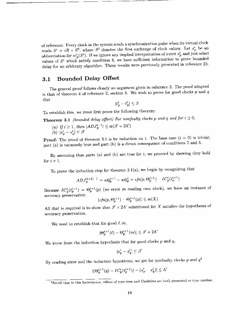
of reference.Everyclockin thesystemsendsasynchronizationpulsewhenits virtual clocki beanreadsS i = iR + S °, where S o denotes the first exchange of clock values. Let sp
i and just selectabbreviation for icip(Si). If we ignore any implied interpretation of event spvalues of S _ which satisfy condition 8, we have sufficient information to prove bounded
delay for an arbitrary algorithm. These results were previously presented in reference 23.
3.1 Bounded Delay Offset
The general proof follows closely an argument given in reference 2. The proof adapted
is that of theorem 4 of reference 2, section 6. We wish to prove for good clocks p and q
that
Lt;- t;I <_
To establish this, we must first prove the following theorem:
Theorem 3.1 (bounded delay offset) For nonfaulty clocks p and q and for i > O,
(a) If i > 1, then IADJp-ll < (_(_' + 2A')
(b) 14 - < 9'Proof: The proof of theorem 3.1 is by induction on i. The base case (i = 0) is trivial;
part (a) is vacuously true and part (b) is a direct consequence of conditions 7 and 5.
By assuming that parts (a) and (b) are true for i, we proceed by showing they hold
for i+ 1.
To prove the induction step for theorem 3.1(a), we begin by recognizing that
ADJ(_+I)-I .... i+l adj; = (.,);+1)_ iC;(t;+l_ ua3p cfn(p, )
Because i i+1 O; +l(p) (no error in reading own clock), we have an instance ofICp(tp )=
accuracy preservation:
lefn(p,O;+ 1) - O;+1 (p)l < ct(X)
All that is required is to show that _' + 2A' substituted for X satisfies the hypotheses of
accuracy preservation.
We need to establish that for good/?, m
i%+,(e)_ o;+l(m)L< + 2A'
We know from the induction hypothesis that for good clocks p and q,
is;- 41-<9'
By reading error and the induction hypothesis, we get for nonfaulty clocks p and q4
I(Ov+l (q) - ICp(tp+l)) - (.Sip - Sq)l <_ M
4Recall that in this formulation, values of type time and Clocktime are both promoted to type number.
18
We proceed as follows:
Je;+l(e) - e;+'(.Oii i+1
= I(%+'(e) - o;+l(m)) + (IC;(tp) - IC;(t;+l))
+ (_; - _;) + (_ - _) + (_ -sL)l
< Isl- sLI + I(e_+_(e) _ g÷l- IG(t , )) - (s; - s_)l+ I(e_+,(_) _ _+1- zc,(t, )) - (s; -s_)l
_< /31 + 2A I
We get the last step by substituting g and rn for p and q, respectively, in the induction
hypothesis, then by using reading error twice, and by substituting first g for q and thenrn for q.
The proof of the induction step for theorem 3.1(b) proceeds as follows. All supporting
lemmas introduced in this section implicitly assume that theorems 3.1(a) and 3.1(b) areboth true for i and that theorem 3.1(a) is true for i + 1. In the presentation of Welch and
Lynch (ref. 2), they introduce a variant of precision enhancement. We restate it here inthe context of the general protocol:
Lemma 3.1.1 For 9ood clocks p and q,
I(sip - Sq) - (ADJ; - ADJ_q)I <_7r(2A' + 2, J + 2A')
Proof: We begin by recognizing that AD,lip = cfn(P,(Ag.O;+l(g) -- ICp(tpi i+l))) (and sim-ilarly for ADJq). A simple rearrangement of the terms gives us
I(s; - Sq) - (ADJ; - ADJq)[ = I(ADJ; - s;) -(aDJq - Sq)[
We would like to use translation invariance to help convert this to an instance of precision
enhancement. However, translation invariance only applies to values of type CIocktime (a
and i to integer values whilesynonym for integer). We need to convert the real values sp Sqpreserving the inequality. We do this via the integer floor and ceiling functions. Without
loss of generality, assume that (ADJip - @) > (ADJq s __ -. q). Thus
I(ADJip - sip)- (ADJ; - Sq)]
<_ I(ADJp - [@J) - (ADJq - rs;1)l= Icfn(p,(M.Oij,(g) i i+1-zc;(t, )- L_ipJ))
-cfn(q,(Ag.oiq+l(g) i i+l- _rcq(tq ) - [s;1))l
All that is required is to demonstrate that if
(ag.O;+' (t) i i+1- Ic_(t_ ) - ksipJ)=
19
and
- ICq(tq )- =(ae.e;+,(e) ,_+1 rs;]) 0
they satisfy the hypotheses of precision enhancement.
We know from reading error and the induction hypothesis that
[(]i(ti+l)) -- (8_,- S}) I < A tI(e;+' (e)- _vp,_p
To satisfy the first hypothesis of precision enhancement, we notice that
ICq (tq --ICp(tp ) Lsgj)(e) (e)- ) [Sql)(e)li(Ae.e;+,(e) , _+1_ _(ae.e;+, _ _+,= -- ICp(tp ) Is;J) (g) IC;(tq +1) - [Sq])li(e;+l(e) _ ,+1 _ _ (e;+_ _= ICp(tp )) - (Ls;] - _D)i((e;+,(e)_ , _+,
lc_w+')) (rsU sD)l--(((F); +' (e) -- --vq,-q -- --
< 25' + 2
Therefore, we can substitute 2A' + 2 for X to satisfy the first hypothesis of precision
enhancement.
To satisfy the second and third hypotheses, we proceed as follows (the argument pre-
ICp(tp ) - [s;]) = 7). We need a value of Y such thatsented is for (Af.O_ +1(£) - i i+1
- ICp(tp ) - Ls;J)(m)I< Yr_W+' - Ls;j)(e) (Ae.e;+'(e)- _ '+'I(Ae.e;+'(e) - __p,_
We know that
rc:iw+_) Ls;J)(m)li(Ae.e;+'(e)- IC;(t; +') - Ls;J)(e)- (At.e;+'(_) - -_p,_p -zcp(% )- Ls_J)l= ICp(tp )-Ls;J)-(e;+_(,_) - , i+1i(e;+l(e)_ _ i+1
-- le;+'(e)- _'+'(,_)1
Tile argument in theorem 3.1(a) shows that this value is bounded by/3' + 2A' which is the
desired Y for the remaining hypotheses of precision enhancement. •
Now we bound the separation of ic;+l(z) and icq+l(T) for all T.
Lemma 3.1.2 For good clocks p and q and clock time T,
[icip+l(T) _ ic;+l(T)] <_ 2p(IT - S i] + tx(/3' + 25')) + zr(2A' + 2,/3' + 2A')
Proof." The proof is taken verbatim (with the exception of notational differences) from
reference 2, lemma 10.
Note that
icip+l(T) = icip(T - ADJ,,) and icq4-'(T) = icq(T- ADJq)
2O
Now
_< ]icp(T- ADjip) - .sip _ (T- ADJ,, - Si)]
+lief,(T- ADJ,)- .Sq - (T- ADJq - S')I
+l(sp - Sq)- (ADJ_ - ADJq) I
Tile three terms are bounded separately. By corollary 5.3 of bounded drift (condi-tion 5), we get
licip(T - AD.I i )p- ,sp'i_ (T- ADJ_ - Si)[
<_ piT- S': - ADJip[
<_ p(lT - Nil + o_( "3' + 2A'))
from theorem 3.1 (a) for i + 1. The second term is similarly bounded. Lemma 3.1.1 bounds
tile third term. Adding the bounds and simplifying gives the result. •
This leads to the desired result:
Lemma 3.1.3 For" .qood clocks p and q,
Is; -Sq+'l 2p(R + _(.'3' + 2A')) + zr(2A' + 2,_'+ 2A') _< fl'
Proof: This is simply an instance of lelmna 3.1.2 wit:h S i+l substituted for T.
This completes the proof of theorem 3.1. Algebraic manipulations on the inequality
2p(R + c_(.'3' + 2A')) + rr(2A' + 2, _3' + 2A') _</3'
give us an upper bound for R.
3.2 Bounded Delay for Two-Algorithm Schemata
VVe begin by noticing that both instantaneous adjustment schemata presented at the
beginning of this chapter allow for a simple derivation of/3 that, satisfies the condition of
bounded delay (Shankar's condition 4). Notice that knowledge of the algorithm is required
in order to flflly establish this property.
Theorem 3.2 (bounded delay) For nonfaulty clocks p,q employing either of the two
instantaneous adjustment schemata presented, there is a '3 such that,
It; - t;I _<
Proof." It is important to remember that 'vti+l = _'ci_pilp'_i+l) = hp-'i+l t_i+l_p + ADJp).
21
1. WhenT_ +1 = (i + 1)R + T °, let/3 = 2p(R - (S O - TO)) +/3'
In this case, since Tp +1 = Tq +1 = (i + 1)R + T °, all that is required is a simple
application of corollary 5.2 and expanding the definition of Si; that is, S i = iR + S °.
Itp +1 - t_+l[ <_ ]Sp - Siq[ + 2p((i + 1)R + T O - S i) <_/3' + 2p(R - (S O - TO))
2. When T i+1 = (i + 1)R + T O - ADJp, let/3 =/3' - 2p(S ° - T O)-p
This case requires the observation that Tp+l + A D Jp = Tq +1 + A D J_ = ((i + 1 ) R + To).
By substituting (i+I)R+T ° for T in lemma 3.1.2 and remembering that S i = iR+S °,
we get
Itp +l - tq+ll _< 2p((R - (S O - TO)) + 0@3' + 25')) + ¢r(2A' + 2,/3' + 25')
We know that
2p(R + ct(J + 25')) - 2p(S ° - T °) + ¢r(25' + 2,/3' + 2A') _</3' - 2p(S ° - T °)
Simple algebra completes the proof of this case.
Condition 7 establishes It° - t°l _</3 for both of these schemata.
This result has no impact on the proofs performed by Shankar. The only difference is
that bounded delay is no longer an assumption. However, it is possible that some bounds
and arguments can be improved.
3.3 EHDM Proofs of Bounded Delay
The EHDM (version 5.2) proofs and supporting definitions and axioms are in the mod-
ules delay, delay2, delay3, and delay4. I-$TEX-formatted listings of these modules are in
appendix B. A slightly modified version of Shankar's module clockassumptions is also
included in appendix A for completeness. Some of the revised constraints presented in
Chapter 2 are in module delay. The most difficult aspect of the proofs was determining a
reasonable predicate to express nonfaulty clocks. Since we would like to express transient-
fault recovery in the theory, it is necessary to avoid the axiom correct _closed from Shankar's
module clockassumptions. This axiom has not yet been removed from the general theory.
None of the proofs of bounded delay offset depend on it, however. The notion of nonfaulty
clocks is expressed by the following from module delay:
correct_during: function[process, time, time ---* bool] =
(Ap, t,s :t < s A (Vh :t _< tl At1 < s D correct(p, tl)))
wpred: function[event --* function[process --* bool]]
rpred: function[event --* function[process _ bool]]
wvr_pred: function[event _ function[process _ bool]] =
(Ai: (tp: wpred(i)(p) V rpred(i)(p)))
wpred_ax: Axiom count(wpred(i), N) >_ N - F
wpred_correct: Axiom wpred(i)(p) D correct_during(p, tp, t_+1)
22
wpred_preceding: Axiom wpred(i -I- 1)(p) D wpred(i)(p) V rpred(i)(p)
wpred_rpred_d isjoi nt: Axiom _ (wpred (i) (p) A rpred (i) (p))
wpred_bridge: Axiom
wvr_pred(i)(p) A correctduring(p, t; +1, t;+ 2) D wpred(i + 1)(p)
Also, module delay3 states the following axiom:
recovery_lemma: Axiom
delay_pred(i) A ADJ_pred(i + 1)
A rpred(i)(p) A correct_during(p tg +1 ' tg+2) A wpred(i + 1)(q)Dis;+1_ s
There are two predicates defined, wpred and rpred. Wpred is used to denote a working
clock; that is, it is not faulty and is in the proper state. Rpred denotes a process that
is not faulty but has not yet recovered proper state information. Correct is a predicate
taken from Shankar's proof that states whether a clock is fault free at a particular in-
stance of real time. Correct_during is used to denote correctness of a clock over an interval
of time. In order to reason about transient recovery it is necessary to provide an rpred
that satisfies these relationships. If we do not plan on establishing transient recovery, let
rpred(i) = (Ap : false). In this case, axioms recovery_lemma and wpred_rpred_disjoint are
vacuously true, and the remaining axioms are analogous to Shankar's correct_closed. This
reduces to a system in which tile only correct clocks are those that have been so since the
beginning of the protocol. This is precisely what should be true if no recovery is possible.
The restated property of bounded drift is captured by axioms RATE_I and RATE 2.
Tile new constraints for bounded interval are rts_new_l and rts new 2. Bounded delay
initialization is expressed by bnd_delay_init. The third clause of the new reading error is
reading_error3. Tile other two clauses are not used in this proof. An additional assump-
tion not included in the constraints given in Chapter 2 is that there is no error in reading
your own clock. This is captured by read_self. All these can be found in module delay.In addition, a few assumptions were included to define interrelationships of some of theconstants required by the theory.
The statement of theorem 3.1 is bnd_delay_offset in module delay2. The main step
of the inductive proof for theorem 3.1(a) is captured by good_Readclock, which with ac-
curacy preservation, was sufiqcient to establish bnd_delay offset_ind_a. Theorem 3.1(b)is more involved. Lemma delay_prec_enh in module delay2 is tile machine-checked ver-
sion of lemma 3.1.1. Module delay3 contains tile remaining proofs for theorem 3.1(b).Leinma 3.1.2 is presented as bound_future. Tile first two terms in the proof are bounded
by lemma bound_futurel; tile third, by delay_prec_enh. Lemma bound_FIXTIME completesthe proof.
Module delay4 contains the proofs that each of the proposed substitutions for fl satisfy
the condition of bounded delay. Option 1 is captured by optionl_bounded_delay, and op-
tion 2 is expressed by option2_bounded_delay. The EHDM proof chain status demonstrating
23
that all proofobligationshavebeenmet canalsobe foundin appendixB. The task ofmechanicallyverifyingthe proofsalsoforcedsomerevisionsto somehandproofsin anearlierdraft of this paper. Theerrorsrevealedby the mechanicalproof includedinvalidsubstitutionof realsfor integersandarithmeticsignerrors.
Modulenew_basicsrestatesShankar'scondition8 asrts0_newand rtsl_newwith thesubstitutionssuggestedin section2.2.3for r,,(,._ and train. These substitutions are proven
i for each of the proposed algorithm schemata in module rmax_rmin.to bound tip+l - tpThe revised statement of condition 9 can also be found in module new_basics; it is ax-
iom nonoverlap. The modules new_basics and rmax_rmin provide the foundations for a
mechanically checked version of the informal proof of theorem 2.1 given in appendix A.
3.4 New Theory Obligations
This revision to the theory leaves us with a set of conditions that are nmch easier
to satisfy for a particular implementation. Establishing that an implementation is an
instance of this extended theory requires the following obligations:
1. Prove the properties of translation invariance, precision enhancement, and accuracy
preservation for the chosen convergence function
2. Derive bounds for reading error from the implementation (condition 6, clauses 1
and 3)
3. Solve the derived inequalities listed at the end of Chapter 2 with values determined
from the implementation and properties of the convergence function
4. Satisfy tile conditions of bounded interval and nonoverlap by using the derived
values.
5. Identify data structures in tile implementation that correspond to the algebraic
definitions of clocks; show that the structures use([ in the implementation satisfy the
definitions
6. Show that the implementation correctly executes an instance of tile following algo-
rithm schema:
i_--O
do forever {
exchange clock values
determine adjustment for this interval
determine T i+1 (local time to apply correction)
when Ici(t) = Ti+l apply correction; i +-- i 4- 1 }
7. Provide a mechanism for establishing initial synchronization (It ° - tq°l< ¢_'- 2P( s°
- T°)); ensure that/T is as small as possible within the constraints of the aforemen-
tioned inequalities
24
8. If the protocoldoesnot behavein the maturerof either instantaneousadjustmentoptionpresented,it will benecessaryto useanothermeansto establishVi: ItS,-t_l <_._fromVi: Is;- Sq[ < ,_'
Requirement 1 is established ill Chapter 4; requirements 2, 3, 4, 5, and 6 are demonstrated
for an abstract design in Chapter 5; and requirement 7 is established ill Chapter 6. The
inequalities used in satisfying requirement 3 are the ones developed in the course of this
work, even though the proof has not yet been subjected to mechanical verification. The
proof sketch ill appendix A is sufficient for the current development. Requirement 8 is
trivially satisfied because the design described herein uses one of the two verified schemata.
25
Chapter 4
Fault-Tolerant Midpoint as an
Instance of Schneider s Schema
The convergence function selected for the design described in Chapter 5 is the fault-
tolerant midpoint used by Welch and Lynch in reference 2. The function consists of dis-
carding tile F largest and F smallest clock readings 'z, and then determining the midpoint
of the range of the remaining readings. Its formal definition is
cfnMID(p'O)---- [ 0(F+I) -}-20(N-F)J
where O(m) returns the ruth largest element in 0. This formulation of the convergencefunction is different from that used in reference 2. A proof of equality between the two
formulations is not needed because it is shown that this formulation satisfies tile properties
required by Schneider's paradigm. For this function to make sense, we want the number
of clocks in the system to be greater than twice the number of faults, N > 2F + 1. In
order to complete the proofs, however, we need the stronger assumption that N > 3F + 1.
Dolev, Halpern, and Strong have proven that clock synchronization is impossible (without
authentication) if there are fewer than 3F + 1 clocks. (See ref. 3.) Consider a system with
3F clocks. If F clocks are faulty, then it is possible for two clusters of nonfaulty clocks
to form, each of size F. Label the clusters C1 and C2. Without loss of generality, assume
that the clocks in C1 are faster than the clocks in C2. In addition, the remaining F clocks
are faulty and are in cluster CF. If the clocks in Cp behave in a manner such that they
all appear to be fast to the clocks in C1 and slow to tile clocks in C2, clocks in each of the
clusters will only use readings from other clocks within their own cluster. Nothing will
prevent the two clusters from drifting farther apart. The one additional clock ensures that
for any pair of good clocks, the ranges of the readings used in the convergence function
overlap.
This section presents proofs that cfnMiD(p,O) satisfies the properties required by
Schneider's theory. The EHDM proofs are presented in appendix C and assume that a
deterministic sorting algorithm arranges the array of clock readings.
5Remember that condition 1 defines F to be tile maximum number of faults tolerated.
26
The propertiespresentedin this chapterareapplicablefor anyclocksynchronizationprotocolthat employsthe fault-tolerantmidpoint convergencefunction. All that is re-quiredfor a verifiedimplementationisa proof that the functionis correctlyimplementedand proofsthat the otherconditionshavebeensatisfied.The weakformsof precisionenhancementandaccuracypreservationareusedto simplify the argumentsfor transientrecoverygivenin Chapter6.
4.1 Translation Invariance
Recall that translation invariance states that the value obtained by adding CIocktime X
to the result of the convergence function should be the same as adding X to each of the
clock readings used in evaluating the convergence function. The condition is restated here
for easy reference exactly as presented in Chapter 2.
Condition 2 (translation invariance) For arty function 0 mapping clocks to clockvalues,
cfn(p, (An: O(n) + X)) = cfn(p, O) + X
Translation invariance is evident by noticing that for all m,
and
(AI : O(1) + X)(m) = O(m ) + X
(O(F+I) @X)-I-(O(N-F)nt-X))2 = O(F+I) 20(N-F) j+X
4.2 Precision Enhancement
As mentioned in Chapter 2 precision enhancement is a formalization of the concept
that, after executing the convergence fimction, the values of interest should be close to-
gether. The proofs do not depend on p and q being in C; therefore, the precondition was
removed for the following weakened restatement of precision enhancement:
Condition 3 (precision enhancement) Given any subset C of the N clocks with
ICI >_ N - F, then for any readings _/ and 0 satisfying the conditions
1. For any l in C, I'/(1) - O(l)l <_ X
2. For any l, m in C, I (l) - (m)l _<Y
3. For any l, m in C, IO(l) - O(m)l <_ y
there is a bound 7r(X, Y) such. that
[efn(P, 7) - cfn(q,O)l < 7c(X, Y)
27
Theorem 4.1 Precision enhancement is .satisfied for cfnMI D(P, _) if
One characteristic of cfnMID(P, 1)) is that it is possible for it to use readings from faulty
clocks. If this occurs, we know that such readings are bounded by readings from good
clocks. The next few lemmas establish this fact. To prove these lemmas, it was expedient
to develop a pigeonhole principle.
Lemma 4.1.1 (Pigeonhole Principle) If N is the number of clocks in the system and
C1 and C'2 are subsets of these N clocks,
Ic11+1c21 >_N + k IC, nC21 >_k
This principle greatly simplifies the existence proofs required to establish the next two
lemmas. First, we establish that the values used in computing the convergence function
are bounded by readings from good clocks.
Lemma 4.1.2 Given any subset C of the N clocks with ICI >_ N - F and any reading O,
there exist p, q E C such that
O(p) >_ 0(,_+1) and O(N-F) > O(q)
Proof: By definition, I{P: O(p) >__0(f+l)}l >- F + 1 (similarly, I{q : 0(N-F) >-- 0(q)}l >-
F + 1). The conclusion follows immediately from the pigeonhole principle. "
Now we introduce a lemma that allows us to relate values from two different readings
to the same good clock.
Lemma 4.1.3 Given any subset C of the N clocks with IC] >_ N - F and readings 0
and "Y, there exist a, p E C such that
O(p) > 0(N-F) and _/(F+I) - 3'(p)
Proof: With N >_ 3F + 1, we can apply the pigeonhole principle twice: first, to establish
that I{P : O(p) >_ O(N-F)} f) CI _ F -t- 1 and second, to establish the conclusion. "
An immediate consequence of the preceding lemma is that. the readings used in computing
cfnMiD(P, O) bound a reading from a good clock.
The next lemma introduces a useful fact for bounding the difference between good
clock values from different readings.
Lemma 4.1.4 Given any subset C of the N clocks and clock readings 0 and _/ such that
for any l in C, the bound IO(l) -_'(l)l <_ X holds, for all p,q E C,
O(p) >_ O(q) /', "7(q) >_ "/(p) _ IO(p) - _(q)l -< X
28
Proof: By cases,
1. If O(p) >_ 7(q), then [O(p) - 7(q)[ < IO(p) - 7(p)[ _< X
2. If O(p) < 7(q), then [O(p) - 7(q)I -< [O(q) - 7(q)[ _< X •
From this lemma, we can establish tile following lemma:
Lemma 4.1.5 Giwm any subset C of the N clocks and clock readings 0 and 7 such that
for any 1 in C, the bound [O(1) - 7(l)[ < X holds, there, exist p,q C C such that
O(p) >_ 0(_+_)
7(q) > 7(F+1
10(p)- 7(q)l < X
Proof: We know from lemma 4.1.2 that there are Pl,ql C C that satisfy the first twoeonjuncts of the conclusion. Three cases to consider are
1. If 7(p_) > 7(ql) ' let p = q = Pl
2. If O(ql) > O(pl), let p = q = ql
3. Otherwise, we have satisfied the hypotheses for lemma 4.1.4; therefore, we let p = Pland q = ql
We are now able to establish precision enhancement for cfnMlD (p, _9) (theorem 4.1).Proof." Without loss of generality, assume cfnMlt)(p, 7) >_ cfnMID(q,O):
IcfnM1D(p, 7) - cfnMiD(q 0)1
= tlT(F+_)_7(N-FI), 10(_+_)_0(X F)I I
Thus we need to show that
JT(F+I) q- 7(N-F) -- (0(F+I) + O(N-F)) I _ Y + 2X
By choosing good clocks p, q from lemma 4.1.5, Pl from lemma 4.1.3, and ql from the rightconjunct of lemma 4.1.2 we establish
IT(F+I) -_- 7(N_F) -- (0(F+I) _- O(N_F))I
_< 17(q)+7(p_) - 0(p_) - 0(q_)l
= 17(q) + (O(p) - O(p)) + 7(p,) - O(p,) - O(q,) I
< IO(p) - O(q,)l + 17(q) - O(p)[ + 17(p,) - O(p_)l<_ Y+2X
(by hypotheses and lemma 4.1.5).
29
4.3 Accuracy Preservation
Recall that accuracy preservation formalizes the notion that there should be a bound
on the amount of correction applied in any synchronization interval. The proof here uses
the weak form of accuracy preservation. The bound holds even if p is not in C.
Condition 4 (accuracy preservation) Given any subset C of the N clocks with
ICI >_ N- F and clock readings 0 such that, for any l and m in C, the bound
IO(l ) - O(rn)l < X holds, there is a bound a(X) such that for any q in C,
Icfn(p,O) - o(q)l <__,(x)
Theorem 4.2 Accuracy preservation is satisfied for CfnMID(P, O) if c_(X) ---- X.
Proof: Begin by selecting Pl and ql using lemma 4.1.2. Clearly, O(pl) >_ cfnMID(P, O)
and cfnMID(P, O) > 0(ql)- Two cases to consider are
1. If O(q) <_ efnMID(p,O), then leInMID(p,O)- O(q)l <--IO(p 1) -O(q)l < X
2. If O(q) >_ cfnMID(P, 0), then IcfnMID(P, O) -- O(q)l <-- [O(ql) -- O(q)l <-- X "
4.4 EHDM Proofs of Convergence Properties
This section presents the important details of the EHDM proofs that cfnMID(P, O)
satisfies the convergence properties. In general, the proofs closely follow the presentation
given previously. The EHDM modules used in this effort are given in appendix C. Support-
ing proofs, including the EHDM proof of the pigeonhole principle, are given in appendix D.
One underlying assumption for these proofs is that N _ 3F + 1, which is a well-
known requirement for systems to achieve Byzantine fault tolerance without requiring
authentication (ref. 3). The statement of this assumption is axiom No_authentication in
module if_mid_assume. As an experiment, this assumption was weakened to N > 2F + 1.
The only proof corrupted was that of lemma good_between in module mid3. This corre-
sponds to lemma 4.1.3. Lemma 4.1.3 is central to the proof of precision enhancement. Itestablishes that for any pair of nonfaulty clocks, there is at least one reading from the
same good clock in the range of the readings selected for computation of the convergence
function. This prevents a scenario in which two or more clusters of good clocks continue
to drift apart because the values used in the convergence function for any two good clocks
are guaranteed to overlap.
Another assumption added for this effort states that the array of clock readings can
be sorted. Additionally, a few properties one would expect to be true of a sorted array
were assumed. These additional properties used in tile EHDM proofs are (from module
clocksort)
3O
funsort_ax:Axiom
i < j Aj < N D 0(funsort(0)(i)) > 0(funsort(_9)(j))
funsort_tra ns_inv: Axiom
k < N D (_(funsort( A q: _(q) + X)(k)) = v_(funsort(tg)(k)))
cnt_sort_geq' Axiom
k _< N D count((Ap : O(p) > t_(funsort(vg)(k))), N) > k
cnt_sort_Jeq: Axiom
k _< N D count(( ,kp: vg(funsort(vg)(k)) _> vg(p)), N) _> N - k + 1
Appendix C contains the proof chain analysis for the three properties. The proof for
translation invariance is in module mid, precision enhancement is in rnid3, and accuracypreservation is in mid4.
A number of lemmas were added to (and proven in) module countmod. The most
important of these is the aforementioned pigeonhole principle. In addition,lemma count_complement was moved from Shankar's module ica3 to countmod. Shankar's
complete proof was rerun after the changes to ensure that nothing was inadvertently de-
stroyed. Basic manipulations involving the integer floor and ceiling functions are presented
in module floor_ceil. In addition, the weakened versions of accuracy preservation and trans-
lation invariance were added to module clockassumptions. The restatements are axioms
accuracy_preservation_recovery_ax and precision_enhancement_recovery_ax, respectively. The
revised formulations imply the original formulation, but are more flexible for reasoning
about recovery from transient faults because they do not require that the process eval-
uating the convergence function be part of the collection of working clocks. The proofs
that cfnMiD(p,O) satisfies these properties were performed with respect to the revised
formulation. The original formulation of the convergence function properties is retained
in the theory because not all convergence functions satisfy the weakened formulas.
Chapter 5 presents a hardware design of a clock synchronization system that uses
the fault-tolerant midpoint convergence function. The design is shown to satisfy the re-
maining constraints of the theory.
31
Chapter 5
Design of Clock Synchronization
System
This chapter describes a design of a fault-tolerant clock synchronization circuit that
satisfies the constraints of the theory. This design assumes that the network of clocks
is completely connected. Section 5.1 presents an informal description of the design, and
section 5.2 demonstrates that the design meets requirements 2 through 6 from section 3.4.
5.1 Description of Design
As in other synchronization algorithms, this one consists of an infinite sequence of
synchronization intervals i for each clock p; each interval is of duration R + ADJp. All
good clocks are assumed to maintain an index of the current interval (a simple counter is
sufficient, provided that all good channels start the counter in the same interval). Further-
more, the assumption is made that the network of clocks contains a sufficient number of
nonfaulty clocks and that tile system is already synchronized. In other words, the design
described in this chapter preserves the synchronization of the redundant clocks. The issue
of achieving initial synchronization is addressed in Chapter 6. The major concern is when
to begin the next interval; this consists of both determining tile amount of the adjustment
and when to apply it. For this, we require readings of the other clocks in the system and a
suitable convergence function. As stated in Chapter 4, the selected convergence function
is the fault-tolerant midpoint.
In order to evaluate the convergence function to determine the (i + 1)th interval clock,
clock p needs an estimate of the other clocks when local time is Tp +1. All clocks partici-
pating in the protocol know to send a synchronization signal when they are Q ticks into
the current interval; 6 for example, when LCip(t) = Q, where LC is a counter measuring
elapsed time since tile beginning of the current interval. Our estimate, _p(-)i+l, of other
clocks is
0;+1 (q) = T; +1 + (Q- LC;(tpq))
6This is actually a simplification for the purpose of presentation. Clock p sends its signal so lhat it willbe received at the remote clock when LC;,(t) = Q.
32
wheretpq is tile time when p recognizes the signal from q. The value Q - LC]_(tpq) givestile difference between when tile local clock p expected the signal and when it observed
a signal froln q. The reading is taken in such a way that simply adding tile value to the
current local clock time gives an estimate of the other clock's reading at that instant. It
is not important that Q be near the end of tile interval. For this system, we assume tile
drift rate p of a good clock is less than 10 5; this value corresponds to the drift rate of
comlnercially available oscillators. By selecting R to be < 10 4 ticks (a synchronization
interval of 1 insec for a 10-MHz clock), the maxinmm added error of 2pR <_ 0.2 caused by
clock drift does not appreciably alter the quality of our estimate of a remote (:lock's wdue.
hi this system, p always receives a signal from itself when LC_(t) = Q; therefore, no erroris made in reading its own clock.
Chapter 3 presents two options for determining when to apply the adjustment. This
design employs the second option, namely that
Tt*,+l = (i + 1)R + T ° - ADJ;,
Recalling that t_+1 = :_i,:p_Q,_i+l) = _'_i+1(T_+1_> + AD.]_) makes it. easy to determine from
the algebraic clock definitions given in section 2.1 and the above expression, that
cfnMiD(P, (_)p+l) = rr_i+l _,i+1_ rll---p t_p j = (i+l)R+
Since T ° = 0 in this design, we.just need to ensure that cfnM,D(p, fop +1) = (i + 1)R. Using
translation invariance and this definition for (9_ +1 gives
CfilMID(P, (q) _ 1)) = (i + 1)R - T;+1 ----ADJ;,
Since O;+' (q) - Ti+l_p = (Q - LC;(tpq)), we have
ADJ_p = cfllAllD(P, (Xq(Q - LG(tpq))))
In Chapter 4, tile fault-tolerant midpoint convergence function was defined as follows:
@tMiD(p,O) = [O(F+I) +_O(N-F) J
If we are able to select tile (N - F)th and (F + 1)th readings, computing this flmction
in hardware consists of a simple addition followed by all arithinetic shift right. 7 All that
reinains is to determine tile appropriate readings to use. By assumption, there are a suf-
ficient number (N - F) of nonfaulty synchronized clocks participating in the protocol.
Therefore, we know that we will observe at least N - F pulses during the synchronization
interval. Since Q is fixed and LC does not decrease during the interval, the readings
(AqQ- LC_(tpq)) are sorted into decreasing order by arrival time. Suppose tpq is when tile
(F + 1)th pulse is recognized, then Q - LC*p(tpq) must be the (F + 1)th largest, reading.
A similar argulnent applies to the (N - F)th pulse arrival. A pulse counter gives us tile
ran arithmetic shift right of a two's complement value preserves the sign bit an(l Irulwat(,s lh(, le;uslsigififi('ant bit.
33
1 2 N-1 N
Signal Select
l o ° .
I
- +
i
O,
LC
Figure 5.1: Informal block model of clock synchronization circuit.
necessary information to select appropriate readings for the convergence function. Once
N - F pulses have been observed, both the magnitude and time of adjustment can be
determined. At this point, the circuit just waits until LC_(t) = R + ADJp to begin the
next interval.
Figure 5.1 presents an informal block model of the clock synchronization circuit. The
circuit consists of the following components: s
N pulse recognizers (only one pulse per clock is recognized in any given interval)
Pulse counter (triggers events based on pulse arrivals)
Local counter LC (measures elapsed time since beginning of current interval)
Interval counter (contains the index i of the current interval)
One adder for computing the value -(Q - LCp(tpq))
One register each for storing --0(F+I) and --O(N-F)
Adder for computing the sum of these two registers
A divide-by-2 component (arithmetic shift right)
The pulses are already sorted by arrival time, therefore, using a pulse counter is naturalto select the time stamp of the (F + 1)th and the (N - F)th pulses for the computation
_In order to simplify the design, the circuit computes -ADJ], and then subtracts this value when
applying tile adjustment. Thus the readings captured are -0 rather than 0.
34
of the convergence function. As stated previously, all that is required is the differencebetween the local and remote clocks. Let
0 = ()_q.O;+l(q)- T; +1)
When the (F + 1)th (N - F)th signal is observed, register --O(F+1) (--O(N-F)) is clocked,
saving the value -(Q-LCp(t)). After N-F signals have been observed, the nmltiplexor se-
lects the computed convergence function instead of Q. When LCp(t)-(-cfnMJD(p, (0))) =
R, it is time to begin the (i+ 1)th interval. To do this, all that is required is to increment i
and reset LC to 0. Tile pulse recognizers, multiplexor select, and registers are also resetat this time.
5.2 Theory Obligations
The requirements referred to in this section are from the list presented in section 3.4.
Since this design was developed, in part, frSm the algebraic definitions given in section 2.1,
it is relatively easy to see that it meets the necessary definitions as specified by require-ment 5. The interval clock is defined as follows:
IC_(t) = iR + LC_(t)
From the description of the design given, we know that
IF; +1 (t) = IC_(t) + ADJ;_
with LC°p(t) corresponding to PCp(t) as described in Chapter 2. The only distinction is
that, in the implementation, LC is repeatedly reset. Even so, it is the primary mecha-
nism for marking the passage of time. Clearly, this implementation of IC ensures that
this design provides a correct VC. The time reference provided to the local processing
elements is the pair (i, LC_(t)) with the expected interpretation that the current elapsed
time since tile beginning of the protocol is iR + LC_(t).
This circuit cycles through the following states:
1. From LCp(t) = 0 until the (N - F)th pulse is received, it determines the readings
needed for the convergence flmction
2. It uses the readings to compute the adjustment ADJ_
3. When LCp(t)+ADJ_ = R, it applies the correction by resetting for the next interval
In parallel with this sequence of states, when LCp(t) = Q, it transmits its synchro-
nization signal to the other clocks in the system. This algorithm is clearly an instance
of the general algorithm schema presented as requirement 6 (section 3.4). State 1, in
conjunction with the transmission of the synchronization signal, implements the exchangeof clock values. State 2 determines both the adjustment for this interval and the time of
application. State 3 applies the correction at the appropriate time.
35
Requirement 2 demands a demonstration that tile mechanism for exchanging clockvalues introduces at most a small error to the readings of a remote clock. The best that
can be achieved in practice for the first clause of condition 6 is for A to equal 1 tick.
The third clause, however, includes real-time separation and a possible value for A' of
approximately 0.5 tick. We assume these values for tile remainder of this paper. A hard-ware realization of the above abstract design with estimates of reading error equivalent
to these is presented in reference 24. These bounds have not been established formally.
Preliminary research, which may enable formal derivation of such bounds, can be found
in reference 25.
With these values for reading error, we can now solve the inequalities presented at the
end of Chapter 2. The inequalities used for this presentation are those from the informal
proof of theorem 2.1 given in appendix A. These inequalities are
1. 4prmaz + _'([2A' + 2J, L¢_'+ 2A'J) </3'
2. [(1 + p)_' + 2p_,,,_A <_
3. _(L/3' + 2A']) + A + [2pL4] + 1 _< 6
For the first inequality, we need to find the smallest value of /3' that satisfies the
inequality. The bom_d/_' can be represented as the sum of an integer and a real between0 and 1. Let the integer part be /3 and the real part be b. We know that pR < 0.1 and
that r,,,_, is not significantly more than R. Therefore, we can let b = 4prm¢,j: _ 0.4 and
reduce the inequality to the following form:
_([2A' + 2J, kg' + 2A']) < /3
The estimate for A' is _ 0.5 < 1-b/2, therefore with _2A' + 2j = 3 and _/3' + 2A'] =/3+1.
Using the 7r established for cfn_.HD(p, 0) in Chapter 4 gives
3+ -- </3
The smallest value of/3 that satisfies this inequality is 7, therefore, the abow_ circuit can
maintain a value of J that is _ 7.4 ticks. By using this value in the second inequality,
we see that 6 > 8. Because _ is the identity function for cfnMID(P, O) and A = 1, we get
6 > 11 ticks from the third inequality. The bound from the third inequality does not seem
tight, but it is the best proven result we have. By using these numbers with a clock rate of10 MHz, this circuit will synchronize the redundant clocks to within about 1 #sec. Since
the frame length for most flight control systems is on the order of 50 msee, this circuit
provides tight synchronization with negligible overhead.
All that remains in this chapter is to show that this design satisfies requirement 4. This
consists of satisfying conditions 8 and 9. We know that o_(_ _ + 2A _) < 9 and that T ° = 0.
We can satisfy condition 8 by selecting S o such that 9 <_ S ° < R - 9. Since R _ 104, this
should be no problem. For simplicity, let S o = Q. Also, since R >> (1 + p)/3 + _(t3' + 2A'),
condition 9 is easily met. Requirement 7, achieving initial synchronization, is addressed
in the next chapter.
36
Chapter 6
Initialization and Transient
Recovery
This chapter establishes that the design I)resented in Chapter 5 meets the one remain-
ing requirement of the list given in section 3.4. This requirement is to sa.t.is_ _ condition 7,
bounded delay initialization. Establishing this requirement in the absence of faults is suf-
ficient because initialization is only required at system startup. A fault encountered at
startup is not critical and can be remedied by repairing the failed component. However,
a guaranteed automatic mechanism that establishes initial synchronization would provide
a mechanism for recovery from correlated transient failures. Therefore, the arguments
given for initial synchronization attempt to address behavior in the presence of faults also.
These arguments are still in an early stage of development and are therefore presented
informally unlike the proofs in earlier chapters.
Section 6.2 addresses guaranteed recovery from a bounded number of transient faults.
The F, HDM theory presented in section 3.3 presents sufficient conditions to establish
theorem 3.1 while recovering from transient faults. Section 6.2 restates these conditions
and adds a. few more that may be necessary to mechanically prove theorem 2.1 and still
allow transient recovery. Section 6.2 also demonstrates that the design presented in Chap-
ter 5 meets the requirements of these transient recovery conditions.
A mmlber of clock synchronization protocols include mechanisms to achieve initializa-
tion and transient recovery. An implicit assumption in all these approaches is a diagnosis
mechanism that triggers the initialization or recovery action. One goal of this design is
that these fimctions happen autonmtically by virtue of the normal operation of the syn-
chronization algorithm. It appears that the fault-tolerant midpoint cannot be modified to
ensure automatic initialization. However, with slight modification, the fault-tolerant mid-
point algorithnl allows for automatic recovery from transient faults without a diagnosticaction.
37
6.1 Initial Synchronization
If we can get into a state that satisfies the requirements for precision enhancement
(condition 3, repeated here for easy reference):
Condition 3 (precision enhancement) Given any subset C of the N clocks with
ICI > N - F and clocks p and q in C, then for any readings "_ and 0 satisfying the
conditions
1. For any l in C, L_(e) - 0(_)l < X
2. For any l, rn in C, I_/(_) - _/(rn)l <_ Y
3. For any l, m in C, 10(_) - O(m)l <_ Y
there is a bound 7r(X, Y) such that
Icfn(p,"/) - cfn(q,O)l < 7r(X,Y)
where Y < L_read + 2A'J and X = [2A' + 2J 9, then a synchronization system using the
design presented in Chapter 5 will converge to the point where IS°p - s°l <__/T in approx-
imately log2(Y) intervals. Byzantine agreement is then required to establish a consis-
tent interval counter. (For the purposes of this discussion, it is assumed that a verified
mechanism for achieving Byzantine agreement exists. Examples of such mechanisms can
be found in refs. 26 and 27.) The clocks must reach a state satisfying the above con-
straints. Clearly, we would like flread to be as large as possible. To be conservative, we
set _read : (min(Q, R - Q) - c_([fl' + 2A'J))/(1 + p). Figure 6.1 illustrates the relevant
phases in a synchronization interval. If the clocks all transmit their synchronization pulses
within _read of each other, the clock readings will satisfy the constraints listed above. By
letting Q = R/2, we get the largest possible symmetric window for observing the other
clocks. However, more appropriate settings for Q may exist.
R - ADJp4 ................................
Q -- flread _read _read
Figure 6.1: Key parts of synchronization interval.
"This condition is satisfied when for p,q E C, I.sl,- s'ql _< 2read. During initialization, i = 0.
38
6.1.1 Mechanisms for Initialization
In orderto ensurethat wereachastatethat satisfiestheserequirements,it isnecessaryto identify possiblestatesthat violatetheserequirements.Suchstateswould happenbecauseof thebehaviorof clocksprior to the time that enoughgoodclocksarerunning.In previouscases,weknewwehada setC of good clocks with IC I _> N - F. This means
a sufficient number of clock readings were available to resolve O(F+I ) and 0(N F). Thismay not be true during initialization. We need to determine a course of action when we
do not observe N - F clocks. Two plausible options are as follows:
Assumed perfection -- pretend all clocks are observed to be in perfect synchrony
End of interval -- pretend that unobserved clocks are observed at the end of tile syn-
chronization interval; i.e., LCp(tpq) - Q = R - Q; compute tile correction based on
this value
The first option is simple to implement because no correction is necessary. When LC = R,
set both i and LC to 0, and reset the circuit for the next interval. To implement the second
option, perform the following action when LC = R: if fewer than N- F (F+ 1) signals are
observed, then enable register --0(N-F)(--0(F+I)). This causes the unobserved readings to
be (R-Q) which is equivalent to observing the pulse at the end of an interval of duration R.
We discuss these two possibilities with respect to a four-clock system. Tile argu-
ments for the general case are similar, but are combinatorially more complicated. We
only consider cases in which at least one pair of clocks is separated by more than L/re_d.Otherwise, the conditions enumerated would bc satisfied.
6.1.1.1 Assumed Perfection
For assumed perfection, all operational clocks transmit their pulse within (1 + p)R/2
of every other operational clock. We present one scenario consisting of four nonfaulty
clocks to demonstrate that this approach does not work. At least one pair of clocks is
separated by more than 13r_ad. A real implementation needs a certain amount of time to
reset for the next interval; therefore, there is a short period of time z at the end of an
interval where signals will be missed. This enables a pathological case that can prevent
a clock from participating in the protocol, even if no faults are present. If two clocks
are separated by (R - Q) - z, only one of the two clocks is able to read the other. If
additional clocks that are synchronous with the hidden clock are added, they too will be
hidden. Figure 6.2 illustrates a four-clock system caught in this pathological scenario.
The scale is exaggerated to clearly depict the window z in which signals from other clocks
cannot be observed. Typically, this window is quite small with respect to the lengthof the synchronization interval. In this figure, clock a never sees the other clocks in
the system, and therefore remains unsynchronized, even though it is not faulty. There
are a number of options for remedying this deficiency, but all result in more difficult
arguments for demonstrating recovery from transient faults. The presence of this window
of invisibility is unfortunate, because it invalidates a simple probabilistic proof that this
approach guarantees initial synchronization. Although the illustration shows Q = R/2, asimilar pathological scenario exists for any setting of Q.
39
VCa
, rq
Figure 6.2: Pathological scenario---assumed perfection.
V Cd
6.1.1.2 End of Interval
The end of interval approach is an attempt to avoid the pathological case illustrated
in figure 6.2. We begin by considering the cases where only two clocks are actively partic-
ipating. Assume for the sake of this discussion that Q = R/2 (to maximize *qr,,_d). There
are two possibilities--the synchronization pulses are either separated by more than R/2
or less than R/2. The two cases are illustrated in figure 6.3. In case 1, each clock com-
putes tile maxinmm adjustment of R/2 and transmits a pulse every 3R/2 ticks. In case 2,
VCb computes an adjustment of R/4 and transmits a pulse every 5R/4 ticks, whereas
VCa computes an adjustment between R/4 and R/2 and converges to a point where it
transmits a pulse every 5R/4 ticks and is synchronized with VCb. If we add a third clock
to ease 1, it must be within R/2 of at least one of the two clocks. If it is within R/2 of
both, it will pull the two clocks together quickly. Otherwise, the pair within R/2 of each
other will act as if they are the only two clocks in the system and will converge to each
other in tile manner of case 2. Since two clocks have an interval length of 5R/4, and the
third has an interval length of 3R/2, the three clocks will shortly reach a point where they
are within ,/_read of each other. This argument also covers the case where we add a third
clock to case 2. Once the three nonfaulty clocks are synchronized, we can add a fourth
clock and Use the transient recovery arguments presented in section 6.2 to ensure that it
joins the ensemble of clocks. This provides us with a sound mechanism to ensure initial
synchronization in the absence of failed clocks; we just power the clocks in order with
enough elapsed time between clocks to ensure that they have stabilized. This mechanism
is sufficient to satisfy the initialization requirement but does not address reinitialization
due to the occurrence of correlated transient failures.
Unfortunately, if we begin with four clocks participating in the initialization scheme,
a pathological scenario arises. This scenario is illustrated in figure 6.4. Clocks VCa and
40
VCb are synchronized with each other in the manner of case 2 of figure 6.3; likewise, VCc
and l/Cd are synchronized. The two pairs are not synchronized with each other. This
illustrates that even with no faulty clocks, the system may converge to a 2-2 split: two
pairs synchronized with each other but not with the other pair. Once again, values for Q
other than R/2 were explored; in each case a 2-2 split was discovered. The next section
proposes a means to avoid this pathCogical case, while preserving the existing m(_ans forachieving initial synchronization and transient recovery.
..... R ..... _'q" ADJ" "_
........ 3R/2 ........
÷ I I
Case 1: [.s_ - sbl >_ tff2
" ...... 517/4 ....... "
Case 2: I,_',,-._'_t < R/2
Figure 6.3: End of interval initialization.
VCb
6.1.1.3 End of Interval--Time-Out
Inspection of figure 6.4 suggests that if any of the clocks were to arbitrarily decide not
to compute any adjustment, the immediately following interval would have a collection of
three clocks within /_¢_,t of each other, as shown in figure 6.5. When clock b decides not
to compute any adjustment, it shifts to a point where its pulse is within 3_,,_d of c and d.
tlere the algorithm takes over, and the three values converge. Figure 6.5 illustrates the
fault-free case. If a were faulty, it. couM delay converg(_nce by at most log2(/]r(,_,t ). Clock a
is also brought into the fold because of the transient recovery process. This process is
explained in more detail in section 6.2. All that remains is to provide a means for the
(:locks not to apply any adjustment when such action is necessary.
Suppose each clock maintains a count of the Immber of elapsed intervals since it has
observed N - F pulses. When this count reaches 8, for example, it is rea_sonably safe
41
VCa
VCb
_ VCc
÷ ÷
Figure 6.4: Pathological end of interval initialization.
_ VCd
Iflread
VCa
I VCb
VCd
Figure 6.5: End of interval initialization--time-out.
42
to assume that either fewer than N - F clocks are active or the system is caught in the
pathological scenario illustrated in figure 6.4. In either case, choosing to apply no correc-
tion for one interval does no harm. Once this time-out expires, it is important to reset
the counter and switch back immediately to the end of interval mode. This prevents the
system from falling into the pathological situation presented in figure 6.2.
Now that we have a consistent mechanism for automatically initializing a collection
of good clocks, we need to explore how a faulty clock could affect this procedure. First
we note that figure 6.4 shows the only possible pathological scenario. Consider that an
ensemble of unsynchronized clocks must have at least one pair separated by more than
._read, otherwise the properties of precision enhancement force the system to synchronize.
In a collection of three clocks, at least one pair must be within _r_d; figure 6.3 shows that
in the absence of other readings, a pair within [:lr,,,_dwill synchronize to each other. The
only way a fourth clock can be added to prevent system convergence is the pathological
case in figure 6.4. If this fourth clock is fault free, the time-out mechanism will ensure
convergence. Two questions remain: can a faulty clock prevent the time-out from expir-
ing, and can a faulty clock prevent synchronization if a time-out occurs. We address theformer first.
Recall from the description of the design that, in any synchronization interval, each
clock recognizes at most one signal from any other clock in the system. The only means
to prevent a time-out is for each nonfaulty clock to observe three pulses in an interval,
at least once every eight intervals. In figure 6.6, d is faulty in such a manner that it will
be observed by a, b, and c without significantly altering their computed corrections. This
fault is considered benign because d is regularly transmitting a synchronization pulse that
is visible to all the other clocks in the system. Clock d is considered faulty because it is
not correctly responding to the signals that it observes. Clock c is not visible to either a
or b, and neither of these is visible to c. Neither a nor b will reach a time-out, because
they see three signals in every interval. However, except for very rare circumstances,
c will eventually execute a time-out, and the procedure illustrated in figure 6.5 will causea, b, and c to synchronize.
There is one unlikely scenario when Q = R/2 in which the good clocks fail to converge.
It requires c to observe a at the end of its interval, with neither a nor b observing c. Only
one of the symmetric cases is presented here. This is only possible if c and a are separated
by precisely R/2 ticks. Even then, a will more likely see c than the other way around.
This tendency can be exaggerated by setting Q to be slightly more than R/2, ensuring
that a will see c first. If a observes c, the effect will be the same as if it had a time-out.
Since a is synchronized with b, observing c at the beginning of the interval will cause the
proper correction to be 0, and the system will synchronize.
The only remaining question is whether a faulty clock can prevent the others from
converging if a time-out occurs. Unfortunately, a fault can exhibit sufficiently malicious
behavior to prevent initialization. We begin by looking back at figure 6.5. If a is faulty,
and a time-out occurs for b, then b, c, and d will synchronize. If, on the other hand, d
is faulty, we do not get a collection of good clocks within /3r_._d. A possible scenario is
43
t_. VCa
VCb
VCc
................. __:.................. ,_:......... vcd
Figure 6.6: End of interval initialization: d faulty--benign.
From d Front d From d
Froill d From d From d
N , H HFrom d From d From d
.............................................. VCd
Figure 6.7: End of interval initialization: d faulty--malicious.
shown in figure 6.7, where d prevents a from synchronizing and also causes the time-out
for a to reset. At some point, d also sends a pulse at the end of an interval to either b
or c to ensure that just one of them has a time-out. The process can then be repeated,
preventing the collection of good clocks from ever becoming synchronized. This fault ismalicious because the behavior of d appears different to each of the other clocks in the
system.
44
The attempt for a flllly automaticinitialization schemehas fallenshort. A soundmechanismexistsfor initializingtheclocksin the absenceof any failures.Also,if a clockfailspassive,theremainingclockswill beableto synchronize.Unfortunately,thetechniqueis not robustenoughto ensureinitializationin thepresenceof maliciousfailures.
6.1.2 Comparison With Other Approaches
Tileargumentthat theclocksconvergewithin log2(.2Fo_,t)intervalsisadaptedfromthatgivenbyWelchandLynch(ref.2). However,theapproachgivenherefor achievinginitialsynchronizationdiffersfrommostmethodsin that first the intervalclocksaresynchronized.and thenan indexis decidedon for the current interval. Techniquesin references2, 41and6 all dependon the goodclocksknowingthat they wishto initialize. Agreementisreachedamongthe clockswishingto join, andthen the initialization protocolbegins.Itseemsthat.this standardapproachis necessaryto ensureinitializationin the presenceofmaliciousfaults. Theapproachtakenhereis similar to that mentionedin reference20;
however, details of that approach are not given.
6.2 Transient Recovery
The argument for transient recovery capabilities hinges on the following observation:
As long as there is power to the circuit and no faults are present, the circuitwill execute the algorithm.
With the fact that the algorithm executes continually and that pulses can be observed dur-
ing the entire synchronization interval, we can establish that up to F transiently affected
channels will automatically reintegrate themselves into the set of good chmmels.
6.2.1 Theory Considerations
A number of axiolns were added to the EHDM clock synchronization theory to provide
sufficient conditions to establish transient recovery. Current theory provides an uninstan-
tiated predicate rpred that must imply certain properties. To formally establish transient
recovery, it is sufficient to identify an appropriate rpred for the given design and then show
that a clock will eventually satisfy rpred if affected by a transient fault (provided that
enough clocks were unaffected). The task is considerably simplified if the convergence
function satisfies the recovery variants of precision enhancement and accuracy preserva-
tion. In Chapter 4, it was shown that the fault-tolerant midpoint flmction satisfies those
conditions. The current requirements for rpred are tile following:
1. From module delay3
recovery_lemma: Axiom
delay_pred(i) A ADJ_pred(i + 1)
A rpred(i)(p) A correct_during(p, tip+1 ' tip+2) A wpred(i + 1)(q)- <
2. From module new_basics
delay recovery: Axiom
rpred(i)(p) A wvr_pred(i)(q) D It; +1 i+1
45
3. From module rmax_rmin--
ADJ_recovery: Axiom optionl A rpred(i)(p) D IADJ_I <_ a(Lfl' + 2 * A'])
4. From module delay--
wpred_preceding: Axiom wpred(i + 1)(p) 3 wpred(i)(p) V rpred(i)(p)
wpred_rpred_disjoint: Axiom =(wpred(i)(p) A rpred(i)(p))
wpred_bridge: Axiomwvr_pred(i)(p) A correct-during(p, tip+1 ti+_) 3 wpred(/+ 1)(p),-p
The conditions from module delay define wpred; they ensure that a clock is considered
working only if it was working or recovered in the previous interval. They were previ-
ously discussed in section 3.3. Arguments for transient recovery hinge on the first three
constraints presented. In Chapter 3, two options were presented for determining when to
apply the adjustment. These options are
1. Tp +1 = (i+I)R+T O
2. Tp +1 = (i + 1)R + T O- ADJp
Since the design presented in Chapter 5 uses the second option, the arguments for tran-
sient recovery are specific to that case. The argument for this option depends primarily
on satisfying axiom recovery_lernma.
Axiom recovery_lemma is used in the inductive step of the machine-checked proof of
theorem 3.1. To prove recovery_lemma, it is sufficient for rpred(i)(p) to equal the following:
correct_during(p, Sp, tip+l )
wpred(i)(q) 3 ISp - Sql <_ _read and
-_wpred(i)(p)
Using arguments similar to the proof of theorem 3.1, we can then establish that
IADJ_I <_ c_(_re.a + 2A')
licip+l(T) - ic +l(T)l <_2p(IT - S'I + + 2A')) + =(2A' + 2,Z' + 2A')
The second of these is made possible by using the recovery version of precision en-
hancement. Since fl_ > 4prma= + 7r(2A _ + 2, fit + 2A_), all that remains is to establish
that 2p(IS _+_ - S_I + (x(_3re_d + 2A')) <_ 4prmaz. Since /_re'a_l< R/2 and (x is the identity
function, this relation is easily established. Axiom delay_recovery is easily established for
implementations by using the second Mgorithm schema presented in Chapter 3. Because
Tp +1 + ADJp = (i + 1)R + T O and t i+1 = icip+l((i + 1)R + To), all that is required is to-p
substitute (i + 1)R + T O for T in item 2. Since the two options are mutually exclusive and
the design employs the second, axiom ADJ_recovery is trivially satisfied.
46
6.2.2 Satisfying rpred
The only modification required to the design is that the synchronization signals include
tile sender's value for i (the index for the current synchronization interval). By virtue of
the maintenance algorithm, the N - F good clocks are synchronized within a bounded
skew _ << R. A simple majority vote restores the index of the recovering clock. If the
recovering clock's pulse is within flFe_d of the collection of good clocks, rpred is satisfied.
If not, we need to ensure that a recovering clock will always shift to a point where it is
within flre_d of the collection of good clocks.
The argument for satisfying rpred is given for a four-clock system; the argument for
the general case requires an additional time-out mechanism to avoid pathological cases.
Consider the first full synchronization interval in which the recovering clock is not faulty.
In a window of duration R, it will obtain readings of the good clocks in the system. If
the three readings are within 6 of each other, the recovering clock will use two of the
three readings to compute the convergence function, restore the index via a majority vote,
and will be completely recovered for tile next interval. It is possible, however, that the
pulses from the good clocks align closely with the edge of the synchronization interval. The
recovering clock may see one or two clocks in the beginning of the interval and read the rest
at the end. It is important to be using the end of interval method for resolving the absence
of pulses. By using the end of interval method, it is guaranteed that some adjustment
will be computed in every interval. If two pulses are observed near the beginning of the
interval, the current interval will be shortened by no more than R- Q. If only one clock is
observed in the beginning of the interval, then either two clocks will be observed at tim end
of the interval or the circuit will pretend they were observed. In either case, the interval
will be lengthened by (R - Q)/2. It is guaranteed that in the next interval the recovering
clock will be separated from the good clocks by _ (R-Q)/2. Since (R-Q)/2 < fl_e_d, the
requirements of rpred have been satisfied. It is important to recognize that this argument
does not depend on the particular value chosen for Q. This gives greater flexibility for
manipulating the design to meet other desired properties.
6.2.3 Comparison With Other Approaches
A number of other fault-tolerant clock synchronization protocols allow for restoration
of a lost clock. The approach taken here is very similar to the one proposed by Welch and
Lynch (ref. 2). They propose that when a process awakens, it observes incoming messages
until it can determine which round is underway and then waits sufficiently long to ensure
that it has seen all valid nlessages in that round. It then computes the necessary correction
to become synchronized. Srikanth and Toueg (ref. 6) use a similar approach modified to
the context of their algorithm. Halpern et al. (ref. 4) suggest a rather complicated protocol
which requires explicit cooperation of other clocks in the system. All these approaches
have the common theme, namely, that the joining clock knows that it wants to join. This
implies the presence of some diagnostic logic or time-out mechanism that triggers the
recovery process. The approach suggested here happens automatically. By virtue of the
algorithm's execution in dedicated hardware, there is no need to awaken a process to
participate in the protocol. The main idea is for the recovering process to converge to a
state where it will observe all other clocks in the same interval and then restore the correctinterval counter.
47
Chapter 7
Concluding Remarks
Clock synchronization provides tile cornerstone of many fault-tolerant computer ar-
chitectures. To avoid a single point failure it is imperative that each processor maintain a
local clock that is periodically resynchronized with other clocks in a fault-tolerant manner.
Reasoning about fault-tolerant clock synchronization is complicated by the potential for
subtle interactions involving failed components. For critical applications, it is necessary to
prove that this function is implemented correctly. Shankar (NASA CR-4386) provides a
mechanical proof (using EHDM) that Schneider's generalized protocol (Tech. Rep. 87-859,
Cornell Univ.) achieves Byzantine fault-tolerant clock synchronization if 11 constraints
are satisfied. This general proof is quite useful because it simplifies the verification of
fault-tolerant clock synchronization systems. The difficult part of the proof is reusable;
all that is required for a verified system is to show that the implementation satisfies the
underlying assumptions of the general theory. This paper has revised the proof to sim-
plify the verification conditions and illustrated the revised theory with a concrete example.
Both Schneider and Shankar assumed the property of bounded delay. (This termi-
nology is from Shankar's report; Schneider called this property a reliable time source.)
This property asserts that there is a bound on the elapsed time between synchronization
actions of any two good clocks. For many protocols, it is easy to prove synchronization
once bounded delay has been established. For these protocols, the difficult part of the
proof has been left to the verifier. This paper presents a general proof of bounded delay
from suitably modified versions of tile remaining conditions. This revised set of conditions
greatly simplifies tile use of Schneider's theory in the verification of clock synchronization
systems. In addition, a set of conditions sufficient for proving recovery from transient
faults has been added to the theory. A design of a synchronization system, based on the
fault-tolerant midpoint convergence function, was shown to satisfy the constraints of the
revised theory.
One of the goals of the design was to develop a synchronization system that could au-
tomatically initialize itself, even in the presence of faults. Two approaches for a four-clock
system were explored and shown to possess pathological scenarios that prevent reliable
initialization. An informal sketch of a third approach was given that combines techniques
from the two failed attempts. This technique ensures automatic initialization in the ab-
sence of failures or when the failures are benign. However, malicious behavior from a
48
failedclockCallpreventgoodclocksfrom synchronizing.Tile standardapproachof firstreachingagreementandthensynchronizingseemsnecessaryfor guaranteedinitializationill tile presenceof arbitrary failures.
In keepingwith the designphilosophyof tile ReliableComputing Platform (RCP),
the clock synchronization system was designed to recover from transient faults. Sufficient
conditions for transient recovery were embedded in the EHDM proofs. These conditions
were based on the approach used by DiVito, Butler, and Caldwell for the RCP (NASA
TM-102716). It. was shown that a four-clock instance of the given design will satisfv the
transient recovery assumptions. Furthermore, the recovery happens automatically; thereis no need to diagnose occurrence of a transient fault.
In sunmmry, a mechanically checked version of Schneider's paradigm for fault-tolerant
clock synchronization was extended both to simplify verification conditions and to al-
low for proven recovery from transient faults. Use of the extended theory was illustrated
with the verification of an abstract design of a fault-tolerant clock synchrolfization system.
Some of the requirements of the theory were established via a mechanically checked formal
proof using EHDM, whereas other constraints were demonstrated informally. Ultimately, a
mechanically checked argument should be developed for all the constraints to help clarify
the underlying assumptions and, in many cases, to correct errors in tile informal proofs.
Mechanical proof is still a difficult task because it is not always clear how to best present
arguments to the Inechanical proof system. For example, the arguments given for initial
synchronization need to be revised considerably before a mechanically checked proof is
possible. Nevertheless, even though some conditions were not proven mechanically, de-
veloplnent of the design from the mechanically checked specification has yielded better
understanding of the system than has been possible otherwise.
NASA Langley Research CenterHampton, VA 23681-0(}01July 19 1993
49
Appendix A
Proof of Agreement
This appendix consists of two parts: The first part consists of an informal proof sketch
that agreement can be established by using the revised constraints on 5 and some of the
intermediate results of Chapter 3 are presented. The second part consists of information
extracted from EHDM that confirms that the mechanical proofs of agreement have been
performed for the minor revisions to Shankar's theory. There are also revised versions of
modules clockassumptions and lemma_final; iemma_final contains the EHDM statement of
theorem 2.1, lemma agreement.
A.1 Proof Sketch of Agreement
This section sketches the highlights of an informal proof that the following constraints
are sufficient to establish theorem 2.1; these arguments have not yet been submitted to
EHDM:
1. 4prmaz + 7r(L2A' + 2]L3' + 2A'J) <_3'
2. [(1 + p)_' + 2pr,,,ax] < 6
3. c_(L3' + 2A'J) + A + [2p/3] + 1 _< 6
The first of these constraints is established in Chapter 3 and is used to ensure that
ISp - Sql < /3'. We can use an intermediate result of that proof (lemma 3.1.2) to es-tablish the second of these constraints. The third constraint is obtained by substituting
the revised bounds on the array of clock readings (established in the proof of part (a) of
theorem 3.1) into Shankar's proof. This has not been (tone in the mechanical proof be-
cause Shankar's proof has not yet been revised to accommodate transient recovery.
We now prove the following theorem (from Chapter 2):
Theorem 2.1 (bounded skew) For any two clocks p and q
time t,IVCp(t) - VCq(t)[ <
that are nonfaulty at
To do this, we first need the following two lemmas:
5O
Lemma 2.1.1 For nonfaulty clocks p and q, and max(t_,tq) _< t < min(t_+l,tq+l),
[IC_(t) - IC_(t)l < [(1 + p)_' + 2pr,n..]
Proof: We begin by noticing that ICe(t) i . i i= ICp(,Cp(ICp(t))) (and similarly for ICq).Assume without loss of generality that " i i • i i
ZCp(ICp(t)) < zcq(ICq(t)) << t, and let T = ICq(t).Clearly, T < max(T_ +1 Ti+l). We now have_ , -q
[IC_(t) - ICq(t)l i i= IICp(zcq(T)) _ ' i- ICq(zcq(T)) I
- [IC,v(icq(T) ) i .i_ _ ICv(zc,,(T)) I
< [(1 + p)(licq(T) - ic_,(T)l)]
The final step in tim above derivation is established by corollary 5.1.
All that remains is to establish that lic_(T) - %(T)I _</3'+ 2pr.,.x/(1 + p). Ear-lier, we defined r,,,,,: to be (1 + p)(R + c_(y_' + 2A')). The proof is by induction on i. Fori = 0,
lid,(T) - ic_,(T)l < It° _ t°l + 2p(max(T_<, T_ +') - T °)
_< /3' + 2p(R + _(/3' + 2A'))
For the inductive step, we use lemma 3.1.2 to establish that
liCq+l(T) - ic_+l(T)l <- 2p(IT - S i] + a(fl'+ 2A')) + 7r(2A' + 2,/3' + 2A')
There are two cases to consider: if T < S i+1, this is clearly less than /3'; if T >
S _+1, this is bounded by/3'+ 2p(max(T_+YTq+ 1) _ S_+1). It is simple to establish that
(max(T_+',T_+_)- S'+') _<(n + _(_'+ 2A')).
Lemma 2.1.2 For nonfaulty clocks p and q and t i+1 < t < tp +l
IICiv(t) - ICq+l(t)] < c_([/_' + 2A'J) + A + [2p/3] + 1
Proof Sketch: The proof follows closely the argument given in the proof of case 2 of
_+1 istheorem 2.3.2 in reference 10. The proof is in two parts. First, the difference at tqbounded with accuracy, preservation, and then the remainder of the interval is bounded.
The difference in this presentation is that here the argument to c_ is smaller. •
We can now prove theorem 2.1.
i < t < t; +1Proof Sketch: The proof consists of recognizing that VCp(t) = ICp(t) for tp _This, coupled with nonoverlap and the above two lemmas, assures the result. •
51
A.2 EHDM Extracts
A.2.1 Proof Chain Analysis
The following is an extract of the EHDM proof chain analysis for lemma agreement in
module lemma_final.
................... SUMMARY ..................
The proof chain is complete
The axioms and assumptions at the base are:
clockassumptions. IClock_defn
clockassumptions.Readerror
clockassumptions.VClock_defn
clockassumptions.accuracy_preservation-recovery-ax
clockassumptions.beta_0
clockassumptions.correct_closed
clookassumptions.correct_count
clockassumptions.init
clockassumptions.mu_0
clockassumptions.precision_enhancement-rec°very-ax
clockassumptions.rate_l
clockassumptions.rate_2
clockassumptions.rho_0
clockassumptions.rho_l
clockassumptions.rmax_0
clockassumptions.rmin_0
clockassumptions.rts0
clockassumptions.rtsl
clockassumptions.rts2
clockassumptions.rts_2
clockassumptions.synctime_0
clockassumptions.translation-invariance
division.mult_div_l
division.mult_div_2
division.mult_div_3
floor_ceil.ceil_defn
floor_ceil.floor_defn
multiplication.mult_10
multiplication.mult_non_neg
noetherian[EXPR, EXPR].general_induction
Total: 30
52
The definitions and type-constraintsabsmod.abs
basics.maxsync
basics.maxsynctime
basics.minsync
clockassumptions.Adj
clockassumptions.okay_Reading
clockassumptions.okay_Readpred
clockassumptions.okay_Readvars
clockassumptions.okay_pairs
lemma3.okayClocks
multiplication.muir
readbounds.okaymaxsyncTotal: 12
are:
53
A.2.2 Module lemma_final
lemma_final: Module
Using clockassumptions, lemma3, arith, basics
Exporting all with clockassumptions, lemma3
Theory
p,q,px,p2,ql,q2,p'_,q3, i,j,k: Var nat
l,m,n: Var int
x,y,z: Var number
posnumber: Type from number with ()_ x : x >_ O)
r, s, t: Var posnumber
i tp+1correct_synctime: Lemma correct(p, t) A t < tp + ?'rain _ t <
isynctime_multiples: Lemma correct(p,t) A t >_0 A t < i* rmin D tp > t
synctime_multiples_bnd: Lemma correct(p, t) A t :> 0 D t < tipt/r' ......1+1
agreement: Lemma _ <__rm_n
A# < fis ATr([2*A+2*/3*P] + 1,_S -F [2 * ((Trnax -F _) _:p Jr A)l -F 1)
< 6S
A6S + [2*rmax*P_ +1 <6
Aa(6S+ [2*(rm_x+/3)*P +2*A]+1)+A+[2*t3*p]+1
<6
A t > 0 A correct(p, t) A correct(q, t)
]VCp(t) - VCq(t)l <_ 5
Proof
agreement_proof: Prove agreement from
lemma3_3 {i _- [t/r,_.n] + 1},
okayClocks_defn_Ir {i _ Vt/rmin] + 1, t ,-- t_CS},
maxsync_correa{_ _--t, i _--Vt/_.._A+ 1},synctime_multiples_bnd {p _-- (P _ q)[Vt/rmin] + 1]},
rmin_0,
div_nonnegative {x *- t, y _- rmin},
ceil_defn {x _ (t/rmin)}
synctime_multiples_bnd-proof: Prove synctime_multiples_bnd from
ceil_plus_mult_div {x _-- t, y _-- train},
synctime_multiples {i _-- [t/rmm] + 1},
rmin_0,
div_nonnegative {x _- t, y _-- rm_n},
ceildefn {x _- (t/rm,_)}
54
correct_synctime_proof: Prove correct_synctime from rtsl {t _- t_CS}
synctime_multiples_pred:functionlnat,nat,posnumber -_ bool] -_
_ i( A i,p,t :correct(p,t) At >OAt < i * rmin D tp > t)
synctime_mukiples_step: Lemma
i i >i *correct(p,t) A t _> tp A t _> 0 D t v _ rmi,_
synctime_mukiples_proofi Prove synctime_mukiples from
syncti me_m uIti ples_step
synctime_multiples_step_pred: function[nat, nat, posnumber --, bool] -_
<tAt__0D i >i*r.m_)(A i,p, t : correct(p, t) A tp _ tp _
synctime_multiples_step_proof: Prove synctime_multiples_step from
induction {prop _- ( A i : synctime_multiples_step_pred(i, p, t))},mult_lO {x *- rmi_z},
synctime_O,
rts_l {i _ j(@PI},rmin_O,
correct_closed {s *-- t, t _- t3p_PI+I },
distrib {x *-- j@PI, y ,- I, z _- rmi_},
mult_lident {x _-- train}
End lemma_final
55
A.2.3 Module clockassumptions
clockassumptions: Module
Using arith, countmod
Exporting all with countmod, arith
Theory
N: nat
N_0: Axiom N > 0
process: Type is nat
event: Type is nat
time: Type is number
CIocktime: Type is integer
1, m, n, p, q, Pl, P2, ql, q2, P3, q3: Var process
i, j, k: Var eventx, y, z, r, s, t: Var time
X, Y, Z, R, S, T: Var Clocktime
_, 0: Var function[process _ Clocktime]
5, p, rmin, r,,,ax, J3: number
A, p: ClocktimePC.1 (.2), VC.1 (.2): fu nction [process, time -_ CIocktime]
t .2. function[process, event -_ time]*l'
.2. function[process, event -_ function[process --* Clocktime]](_1 '
IC**_ (*3): function[process, event, time -_ Clocktime]correct: function [process, time --* bool]cfn: function[process, fu nction [process --_ CIocktime] --_ CIocktime]7r: function[CIocktime, CIocktime -_ CIocktime]
c_: function[CIocktime --_ Clocktime]
delta_O: Axiom 6 >_ 0
mu_O: Axiom p _> 0
rho_O: Axiom p >_ 0
rho_l: Axiom p < 1
rmin_0: Axiom rmin > 0
rmax_0: Axiom rmaz > 0
beta O: Axiom fl >_ 0
lamb_O: Axiom A >_0
56
init: Axiom correct(p, O) D PCp(O) >_ 0 A PCp(O) < iz
correct_closed: Axiom s > t A correct(p, s) D correct(p, t)
rate_l: Axiom correct(p,
rate_2: Axiom correct(p,
rts0: Axiom correct(p, t)
rtsl: Axiom correct(p, t)
._)A s > t > Pcp(._) - Pcp(t) <_[(3 - t), (a + p)]
s) A .s _> t D PCp(s) - PUp(f) > L(s - f) . (1 - p)j
/+1 iAt <_ tp D t-- tp <_ rmaa:
At>t i+l Dt i >_ ,,p -- tp _ 'l'rrzi n
rts 0: Lemma correct(p, tp+1) D tp+1 - t i <'p _ 1"max
rts_l' Lemma correct(p,t_ +1) D t_ +' -t_, >_ r.m,_
i irts2: Axiom correct(p, t) A t >_ tq + ,3 A correct(q, t) D t >_ tp
i i<3rts_2: Axiom correct(p, t_) Acorrect(q,t_) _ t, -t_ _,
synctime_0: Axiom t_ = 0
VCIock_defn: Axiom
correct(p, t) A t _> t_, A t < ,,pti+l D VCp(t) = IC;(t)
adS._: function[process, event --_ Clocktime] =
(Ap, i : ( if/> 0 then cfn(p, Oip)-PCp(tip) else 0 end if))
I i a _ICIock defn: Axiom correct(/).t) D Co(t) = PCp(t) + djp
Readerror: Axiom correct(p, tp+') A correct(q t; +1 )
- ICq(tp )l <- A
translation_invariance: Axiom
cfn(p, (Ap, --+ Clocktime : 7(Pi) + X)) = cfn(p,,7) + X
ppred: Var function[process --+ bool]F: process
okay_Readpred: function[function[process --+ Clocktime], number,
function[process _ boo[] --_ bool] =
(A _/, y, ppred: (V l,,n: pored(l) A ppred(m) D I?(l) - _/(m)] < y))
okay_pairs: function[function[process -_ Clocktime],
function[process --_ Clocktime], number,
function[process -_ booI] -_ bool] =
( A "y, 0, x, ppred: ( Vpa : ppred(pa) D [7(P:_) - 0(pa)[ < x))
okay_Readpred_floor: Lemma
okay_Readpred(7, y, ppred) Z) okay Readpred(,y, [yj, pored)
okay_pairs_floor: Lemma
okay_pairs(-,/, 0, x, ppred) D okay_pairs(,y, 0, L-J,ppred)
57
N_maxfaults:Axiom F < N
precision_enha ncement-ax: Axiom
count(ppred, N) _> N - F
A okay_Readpred(y, Y, ppred)
A okay_Readpred(0, Y, ppred)
A okay_pairs(y, 0, X, ppred) A ppred(p) A ppred(q)
D lcfn(P,7) -- cfn(q,O)l <-- 7r(X,Y)
precision_en h a ncement_recovery-ax: Axiom
count(ppred,N) >__N - F
A okay_Readpred(y, Y, ppred)
A okay_Readpred(0, Y, ppred) A okay_pairs(y, 0, X, ppred)
D Icfn(p,Y) - cfn(q,O)l <-- 7r(X,Y)
correct_count: Axiom count(( X p : correct(p, t)), N) > N - F
okay_Reading: function[function[process -_ Clocktime], number, time
--. bool] =
(Ay, y,t:(Vpt,ql:correct(p1, t) A correct(ql, t) D I'Y(pl) - y(ql)l < y))
okay_Readvars: fu nction[fu nction [process --* Clocktime],function[process --* Clocktime], number, time
-_ bool] =
()_y,0, x,t : (Vp3: correct(p3,t) D [Y(P3)- 0(P3)I <-x))
okay_Read pred_Reading: Lemma
okay_Reading(% y, t) D okay_Readpred(% y, ( A p: correct(p, t)))
okay_pairs_Readvars: Lemmaokay_Readvars(% 0, x, t) D okay_pairs(y, 0, x, ( X p : correct(p, t)))
precision_enhancement: Lemma
okay_Reading(% Y, t; -I-1 )
A okay_Reading(0, Y, t_ +1 )
A okay_Readvars(% 0, X, t_+1)
A correct(p, tp +1 ) A correct(q, tp+1 )
D ]cfn(p,y) - cfn(q,O)l < rr(X,Y)
okay_Reading_defn_Ir: Lemma
okay_Reading(% y, t)
D (Vpl,ql : correct(p1, t)A correct(ql,t) D lY(PL)- Y(ql)l--< Y)
okay_Reading_defn-rl: Lemma
( V Pl, ql : correct(p1, t) A correct(ql, t) D I_(Pl) - Y(ql)l -< Y)
D okay_Reading(y, y, t)
okay_Readvars_defn_Ir: Lemma
okay_Readvars(% 0, x, t) D (V P3 : correct(p3, t) D lY(P3) - 0(p3)l _< x)
58
okay_Readvars_defn_rl. Lemma
(Vp:_ : correct(p3, t) D I'_(p3)- O(ps)f <_ x)_ okay_Readvars(% O,x, t)
accu racy_preservation_ax: Axiom
okay_Readpred(_/ X, ppred) A count(ppred, N) > N - F A ppred(p) A ppred(q)Icfn(P, "_) - "_(q)l <- o_(X)
accu racy-preservation_recovery_ax: Axiom
okay_Readpred(-),, X, ppred) A count(ppred, N) > N - F A ppred(q)Icfn(p,'7) - "_(q)r <- o_(X)
Proof
okay_Readpred_floor_pr: Prove okay_Readpred_floor from
okay_Readpred {I _-- l@p2, m _-- m_p2},
okay_Readpred {y _-- [yj},
iabs_is_abs {X _-- _(l@p2) - 7(rn@p2), x _-- 7(/_p2) - _(m@p2)},floor_mon {x +-- iabs(X__p3)},
floor_int {i _ iabs(X_p3)}
okay_pairs_floor_pr: Prove okay_pairs_floor from
okay_pairs {P3 _--p3@p2},
okay_pairs {x +- [xj },
iabs_is_abs {x ,- 3'(p3@p2) - O(p3@p2), X ,-- "y(p3@p2) - O(ps_p2)},floor_mon {x +- iabs(X@p3), y _-- x},
floor_int {i _-iabs(X(@p3)}
precision_enhancement_ax_pr: Prove precision_enhancement_ax from
precision_enhancement_recovery_ax
accuracy_preservation_ax_pr: Prove accuracy_preservation_ax from
accuracy preservation_recovery_ax
okay_Reading_defn rl_pr: Prove
okay_Reading_defn_rl {Pl _-pI@PIS, ql _-q]@PIS} from okay_Reading
okay_Reading_defn_Ir_pr: Prove okay_Reading_defn_Ir from
okay_Reading {p] ,--p]@CS, ql _-qI@CS}
okay_Readvars_defn_rl_pr: Prove okay_Readvars_defn_rl {p:_, +- p3@P 1S } fromokay_Readvars
okay-Readvars_defn_Ir_pr: Prove okay_Readvars_defn_Ir from
okay_Readvars {P3 _--p3_CS}
59
precision_enhancement-pr:Prove precision_enhancement from
precision_enhancement-ax {ppred *-- ( _ q: correct(q, tp+_ ))},
okay_Readpred_Reading {t _- t i+] *-- Y},t_+l' y
okay_Readpred_Reading {t *-- _p , y *-- _/', "f _-- 0},
okay_pairs_Readvars {t *-- tp+I, x _-- X},
correct_count {t _-- tp+I }
okay_Readpred_Reading-pr: Prove okay_Readpred_Reading from
okay_Readpred {ppred _-- ( & p : correct(p, t))},
okay_Reading {Pl _-- I@P1S, ql _- m@P1S}
okay_pairs_Readvars-pr: Prove okay_pairs_Readvars from
okay_pairs {ppred _-- (X p : correct(p, t))}, okay_Readvars {P3 _- p3@PIS}
rts_0_proof: Prove rts_0 from rts0 {t _- tp+1 }
rts_l_proof: Prove rts_l from rtsl {t *--- tp +1 }
End clockassumptions
6O
Appendix B
Bounded Delay Modules
This appendix contains the EHDM proof modules for the extended clock synchro-
nization theory. The proof chain analysis is taken from modules delay4, rmax_rmin, and
new_basics. Module delay4 contains the proofs of bounded delay, whereas rmax_rmin and
new_basics show that the new conditions are sufficient for establishing some of the old
constraints from Shankar's theory. Several lines of tile proof analysis have been deleted.
The pertinent information concerning the axioms at the base of the proof chain remains.
B.1
B.1.1
Proof Analysis
Proof Chain for delay4
Terse proof chains for module delay4
SUMMARY
The proof chain is complete
The axioms and assumptions at the base are:
clockassumptions. IClock_defn
clockassumptions.N_maxfaults
clockassumptions.accuracy_preservationrecovery_ax
clockassumptions.precision_enhancement_recovery_axclockassumptions.rho 0
clockassumptions.translation_invariance
delay. FIX_SYNC
delay. RATE_l
delay. RATE_2
delay. R_FIX_SYNC_O
delay.betaread_ax
61
delay.bnd_delay_initdelay.fix_between_syncdelay.good_read_pred_axldelay.read_selfdelay.reading_error3delay.rts_new_ldelay.rts_new_2delay.synctime0_defndelay.synctime_defndelay.wpred_axdelay.wpred_correctdelay.wpred_precedingdelay3.betaprime_axdelay3.recovery_lemmadelay4.optionl_defndelay4.option2_defndelay4.options_exhausteddivision.mult_div_ldivision.mult_div_2division.mult_div_3floor_ceil.ceil_defnfloor_ceil.floor_defnmultiplication.mult_non-negmultiplication.mult_posnoetherian[EXPK,EXPK].general_induction
Total: 36
B.1.2 Proof Chain for rmax_rmin
Terse proof chains for module rmax_rmin
SUMMARY
The proof chain is complete
The axioms and assumptions at the base are:
clockassumptions. IClock-defn
clockassumptions.accuracy-p reservati°n-rec°very-ax
62
cl°ckassumptions.precision_enhancement_recovery_ax
clockassumptions.rho_0
clockassumptions.translation_invariance
delay. FIX_SYNC
delay.RATE_l
delay. RATE_2
delay.R_FIX_SYNC_O
delay.betaread_ax
delay.bnd_delay_init
delay.fix_between_sync
delay.good_read_pred_axl
delay.read_self
delay.reading_error3
delay.rts new_l
delay.rts_new_2
delay.synctimeO_defn
delay.synctime_defn
delay.wpred_ax
delay.wpred_correct
delay.wpred_preceding
delay3.betaprime_ax
delay3.recovery_lemma
delay4.optionl_defn
delay4.option2_defn
delay4.options_exhausted
division.mult_div 1
division.mult_div_2
division.mult_div 3
floor_ceil.ceil defn
floor_ceil.floor_defn
multiplication.mult_non_neg
multiplication.mult_pos
noetherian[EXPR, EXPR].generalinduction
rmax_rmin. ADJ_recovery
Total: 36
B.1.3 Proof Chain for new_basics
Terse proof chains for module new_basics
63
SUMMARY
The proof chain is complete
The axiomsand assumptionsat the base are:clockassumptions.IClock_defnclockassumptions.N_maxfaultsclockassumptions.accuracy_preservation-recovery-axclockassumptions.precision_enhancement-recovery-axclockassumptions.rho_Oclockassumptions.translation_invariancedelay.FIX_SYNCdelay.RATE_ldelay. RATE_2delay.R_FIX_SYNC_Odelay.betaread_axdelay.bnd_delay_initdelay.fix_between_syncdelay.good_read_pred_axldelay.read_selfdelay.reading_error3delay.rts_new_ldelay.rts_new_2delay.synctimeO_defndelay.synctime_defndelay.wpred_axdelay.wpred_correctdelay.wpred_precedingdelay3.betaprime_axdelay3.recovery_lemmadelay4.optionl_defndelay4.option2_defndelay4.options_exhausteddivision.mult_div_ldivision.mult_div_2division.mult_div_3floor_ceil.ceil_defnfloor_ceil.floor_defnmultiplication.mult_non_negmultiplication.mult_posnew_basics.delay_recoverynew_basics.nonoverlapnoetherian[EXPR,EXPR].general_inductionrmax_rmin.ADJ_recovery
Total: 39
64
B.2 delay
delay: Module
Using arith, clockassumptions
Exporting all with clockassumptions
Theory
P, q, p], ql : Var process
i, j, k: Var event
X, S, T: Var Clocktime
s, t, tl, t2: Var time
7: Var function[process _ Clocktime]/_t, 3read, A/: number
R: Clocktime
betaread_ax: Axiom _' <_ _3re_,!A _read < R/2
ppred, ppredl: Var function[process --, bool]S°: Clocktime
S'i: function/event -_ Clocktime] = (A i : i. R + S cJ)
pc.] (.2): function[process, Clocktime -_ time]
ic**_(.3): function[process, event, Clocktime I, time] =
( A p, i,T : pcp(T - adjp) )
,2. function/process, event --_ time] (Ap, i : iCip(Si)),5'. 1 •
T°: Clocktime
T**2: function[process, event --, Clocktime]
synctime_defn. Axiom t_+] i i i+I= Cp(Tp )
0 = icO(T o)synctime0_defn: Axiom tp
FIX_SYNC: Axiom S ° > T °
R_FIX_SYNC_0: Axiom R > (S ° - T °)
R_0: Lemma R > 0
good_read_pred: function[event --_ function[process, process -_ bool]]
correct during: function[process, time, time --, bool] --
(Ap, t,s: t_<7,sA (gtl : t < tl Atl <,s D correct(p, tl)))
wpred: function[event --+ function[process _ bool]]
rpred: function[event --_ function[process --_ bool]]
wvr_pred: fu nction [event -_ function [process --. bool]] =
(A i: (Ap: wpred(i)(p) V rpred(i)(p)))
working: function[process, time -_ bool] =
( A p, t : ( _ i : wpred(i)(p) A t i < t A t < t i+l ))p-- -p
65
wvr_defn:Lemma wvr_pred(i)= (_ p: wpred(i)(p) V rpred(i)(p))
wpred_wvr: Lemma wpred(i)(p) D wvr_pred (i) (p)
rpred_wvr: Lemma rpred(i)(p) D wvr_pred(i)(p)
wpred_ax: Axiom count(wpred(i). N) > N - F
wvr_count: Lemma count(wvr_pred(i). N) :> N -/7
wpred_correct: Axiom wpred(i)(p) D correct_during(p, t_, t¢+1)
wpred_preceding: Axiom wpred(i + 1)(p) D wpred(i)(p) V rpred(i)(p)
wpred_rpred_disjoint: Axiom _(wpred(i)(p) A rpred(i)(p))
wprecl_bridge: Axiom
wv r_pred (i)(p) A correct_d u ri ng(p, t i+1 , tp +2) D wpred (i + 1)(p)
wpred_fixtime: Lemma wpred(i)(p) D correct_during(p, s_, tp +1)
wpred_fixtime-low: Lemma wpred(i)(p) D correct_d uring(p, tp, Sp)
correct_du ring_trans: Lemma
correct_during(p, t, t2) A correct_during(p, t2, s)
D correct_during(p, t, s)
correct_during_sub-left: Lemma
correct_during(p, t, s) A t < t2 A t2 <_ s D correct_during(p, t, t2)
correct_during_sub-right: Lemma
correct_during(p, t, s) A t < t2 A t2 _< s D correct_during(p, t2, s)
wpred_lo_lem: Lemma wpred (i)(p) D correct(p, tp)
wpred_hi_lem: Lemma wpred (i) (p) D correct(p, tp+1)
correct_during-hi: Lemma correct_during(p, t, s) D correct(p, s)
correct_during-Io: [,emma correct_during(p, t, s) Z) correct(p, t)
clock_axl: Axiom PCp(pcp(T)) = T
clock_ax2: Axiom pcp(PCp(t)) <__t A t < pcp(PCp(t) + 1)
iclock_defn: Lemma ic_(T) = pcp(T - adjp)
iclock0_defn: Lemma ic°p(T) = pcp(T)
i - i
iclock_lem: Lemma correct(p, ic_(T)) D ICp(_cp(T)) = T
AD3:._: function[process, event-_ Clocktime] = ()_ P, i: adjp +1 - adj,)
66
ICIock_ADJ_lem:Lemma correct(p,t) D ICp+l(t) = IC;(t) + ADJ_
iclock_ADJ_lem: Lemma _.A+] (T) = ADJ;)
rts_new_l: Axiom correct(p, tp+ 1) D S i + or(L!3' + 2 * A'j) < Tp +j
rts_new_2: Axiom correct(p, tp) D 7p < S i - (_([3' + 2, ArJ)
FIXTIME_bound: Lemma
correct(p, t; +1 ) D S i+1 > S i + 2 * c_([_' + 2 * A'J)
R_bound: Lemma correct(p, t; +l ) _ R > 2 * O_([_' + 2 • A'J)
RATE_l: Axiom correct_during(p, pcp(T), pcp(S)) A S >_ T
D pcv(S ) -- pcp(T) <_ (S- T). (1 + p)
RATE_2:Axiom correct_during(p,p%(T),p%(S)) A S >_ T
D pcp(S) -- pcp(T) > (S - T)/(1 + p)
RAYE_l_iclock: Lemma
c°rrect-during(p, icip(V), icip( s) ) A S >_ T
D icip(S) - icip(T) <_ (S - T). (1 + p)
RATE_2_iclock: Lemma
correct_during(p, icip(T), icip( S) ) A S >_ T
D ic_(S) - iCip(T) >> (S - T)/(1 + p)
rate_simplify: Lemma S _> T D (S- T)/(1 + p) > (S- T). (1 - p)
rate_simplify_step: Lemma S _> T D (1 + p). (S - T). (1 - p) _< S- T
RATE_2_simplify: Lemma
correct_during(p, pcp(T), pCp(S)) A S >_ T
D pcp(S) -pcp(T) >_ (S - T). (1 - p)
RAlE_2_simplify_iclock: Lemma
correct_during(p, i • izcv(T), zcp(S)) A S > T
D icip(s) -- icp(T) > (S - T)* (1 - p)
RATE_lemmal: Lemma
cor rect_d u ring (p, pcp (T) pCp ( S) )
A correct_during(q pcq(T),pCq(S)) A S >_ T
D Ip%(S) - pCq(S)l <_ ]p%(Z) - pcq(r)[ + 2 • p. (S - T)
RATE_lemmal_idock: Lemma
correct_during(p icip(T), iciv( s) )
A correct_during(q, icq(T), icq(S)) A S >_ T
Ii%(s) - ic_(S)l <_lic;(T) - ic_(r)[ + 2 • p. (S - T)
67
RATE_lemma2: Lemma
correct_during(p, pcp(T), pcp( S) ) A S >_ T
D I(p%(S) - S) - (pcp(T) - T)I <_P* (IS- TI)
RATE_lemma2_iclock: Lemma
correct_during(p, iCip(T), iCip(S) ) A S >_ T
D I(icip(S) - S) - (iCip(T) - T)I < p * (IS - TI)
bnd_delayJnit: Axiom
wpred (0)(p) A wpred (0)(q) /3' -pit ° - t°i <_ /3' - 2 * p* (S ° - T O) A - 2 * (p* (S ° - T°)) <
bnd_delay_offJnit: Lemma wpred(0)(p) A wpred(0)(q) D Is° -- s°[ < _'
good_read_pred_axl: Axiomcorrect_during(p, "/ ti+l)up, -p
A correct-during(q,s;,tiq +l) A Isip -- 8;I <_ /3read
D good_read_pred (i) (p, q)
reading_error3: Axiom
good_read-pred (i) (p, q)- ICp(tp )) - (Sp - S_)l <D I(o_+l(q) i i+l " __ A t
ADJ_leml: Lemma correct_during(p, @, t/p+1)
D (ADJp : cfn(p,( _Pl: 0;÷1 (Pl)- [C;(t; +1))))
ADJ_lem2: Lemma correct_during(p, @, t_+1 )
ICp(tp ))D (ADd; = cfn(p, Oip+') - _ i÷1
(_)i÷1 (p) i i+lread_self: Axiom wpred (i) (p) D vp = ICp(tp )
fix_between_sync: Axiomi i A s; < t; +1correct_during(p, tip, tp+1) D tp < 8p
rts_2_lo: Lemma wpred(i)(p) A wpred(i)(q) D It_ - tql < /3
rts_2_hi: Axiom wpred(i)(p) A wpred(i)(q) D ItS,+_ - tq+ll <-
Proof
R_0_pr: Prove R_0 from R_FIX_SYNC_0, FIX_SYNC
FIXTIME_bound-pr: Prove FIXTIME_bound from rts_new_l, rts_new_2 {i *- i + 1}
R_bound_pr: Prove R_bound from FIXTIME_bound, S .1 , S .1 {i *- i + 1}
iclock_defn-pr: Prove iclock_defn from ic*_(*3)
68
wpred_fixtime_pr: Prove wpred_fixtime from
fix_between_sync,
wpred_correct,
i t2_--s_,}correct_during_sub_right {s _ t_+1 , t _ tp,
wpred_fixtime_low_pr: Prove wpred_fi×time_low from
fix_between_sync,
wpred_correct,
correct during_sub_left {s _ t; +!, t _-- t ip, t2 *-- s;}
correct_during_sub_left_pr: Prove correct_during_sub_left from
correct_during {s _- t2}, correct_during {t] _- t](__pl}
correct_during_sub_right_pr: Prove correct_during_sub_right from
correct_during {t _- t2}, correct during {tl *-- t]@pl}
correct_during_trans_pr: Prove correct_during_trans fromcor rect_d u ring,
correct_during {s _- t2, tl *-- t1(@pl},
correct_during {t _-- t2, tl *-- t](_pl}
wpred wvr_pr: Prove wpred_wvr from wvr defn
rpred_wvr_pr: Prove rpred_wvr from wvr_defn
wvr_defn_hack: Lemma
(Vp: wvr_pred(i)(p) = (( A p: wpred(i)(p)V rpred(i)(p))p))
wvr_defn_hack_pr: Prove wvr_defn_hack from wvr_pred {p _- p_c}
wvr_defn pr: Prove wvr_defn from
pred extensionality
{predl *- wvr_pred(i),
pred2 _- (A p: wpred(i)(p)V rpred(i)(p))},
wvr_defn_hack {p _- p¢__pl}
wvr_count_pr: Prove wvr_count from
wpred ax,
count_imp
{ppredl *-- wpred(i),
ppred2 _- (Ap: wpred(i)(p)V rpred(i)(p)),n _- N},
wvr_defn,
imp_pred_or {ppredl _-- wpred(i), ppred2 _-- rpred(i)}
w,x, y, z: Var number
bd_hack: Lemma [w] < x - y A [z I _< Iwl + y D Izl _< x
69
bd_hack_pr: Prove bd_hack
bnd_delay_off_init_pr: Prove bnd_delay_off_init from
bnd_delay_init,RATE_lemmal_iclock {S _- S°, T _- T °, i _- 0},FIX_SYNC,
synctime0_defn,synctime0_defn {p _ q},
.2 {i _- 0},8.1
s .2 {i _-- 0, p _- q},.1
wpred_fixtime_low {i _-- 0},
wpred_fixtirne_low {p _ q, i _- 0},
s .1 {i _- 0}
rnult_abs_hack: Lemma x * (1 - p) <_ y A y < x * (1 + p) _ lY - xl < P * x
mult_abs_hack_pr: Prove mult_abs_hack from
mult_ldistrib {y _ 1, z _ p},
mult_ldistrib_minus {y _ 1, z _ p},
mult_rident,
abs_3_bnd {x _ y, y _ x, z _ p-x},
mult_com {y _ p}
RATE_l_iclock_pr: Prove RATE_l_iclock from
RATE_I {S _-- S - adjp, T _ T - adjp},
iclock_defn,
iclock_defn {T _-- S}
RATE_2_iclock_pr: Prove RATE_2_iclock from
RATE_2 {S _- S- adjp, T _- T- adjp},
iclock_defn,
iclock_defn {T _-- S}
RATE_2_simplify_iclock-pr: Prove RATE_2_simplify_iclock from
RATE_2_simplify {S _- S- adj,, T _ T-adjp},iclock_defn,
iclock_defn {T _ S}
RATE_lemmal_sym: Lemma
correct_during(p, pcp( T), pep(S))
A correct_during(q,pcq(T),pcq(S)) A S > T A pcp(S) > pcq(S)
Ipcp(s) -pcq(S)l < Ipcp(T)-pq(T)l + 2 • p* (S - T)
Rllhack: Lemmaw<xAy <_ zAy>x D lY--X[ < Iz--wl
Rllhack_pr: Prove Rllhack from I* lJ {x _- y - x}, 1" 11 {x _- z - w}
70
RATE_lemmal_sym_pr: Prove RATE_lemmal_sym fromRATE_l,
RATE_2_simplify {p .-- q},Rllhack
{x ,---peq(S),y _-- pep(S),
w *- pcq(T) + (S - T). (1 - p),
z e-- pep(T) + (,_q-- T) * (1 + p)},
mult_ldistrib {x +-- S - T, y _-- 1, z *-- p},
mult_ldistrib_minus {x _-- S - T, y _-- 1, z _- p},
abs_plus {x *-- pep(T) - pcq(T), y _ 2 • p. (S - T)},
mult_com {x*--p, y_-S-T},
abs_geO {x *-- 2 • p. (S - T)},
mult_non_neg {x *--- p, y _-- S - T},rho_0
RATE_lemmal_pr: Prove RATE_lemmal from
RAT E_lem ma l_sym,
RATE_lemmal_sym {p ,- q, q __ p},
abs_com {x *-- pCp(S), y .-- pCq(S)},
abs_com {x _ pep(T), y .- pcq(T)}
RATE_lemma l_iclock_sym. Lemma
correct_during(p, icp( T), iCp( S) )
A correct_during(q, icq(T),ieq(S)) A S >_ T A icip(S) >> icq(S)
D lie_(S) - idq(S)l <_ lic_(T) - icq(T)[ + 2 • p. (S- T)
RATE_lemmal_iclock_sym_pr: Prove RATE_lemmal_iclock_sym fromRATE_l_iclock,
RATE_2_simplify_iclock {p _- q},Rllhack
X ' i
w _ ic_(T) + (S- T). (1 - p),
z _- G(T) + (s - T), (1 + p)},rnult_ldistrib {x *--- S - T, y ,-- 1, z _-- p},
mult_Idistrib_minus {x *-- S - T, y _- I, z *-- p},
abs_plus {x _ icp(T) - ic_(T), y _ 2. p. (S- T)},muir_corn {x _-- p, y _-- S - T},
abs_geO {x _-- 2 * p. (S- T)},
mult_non_neg {x +-- p, y _ S - T},rho_0
71
RATE_lemmal_iclock-pr: Prove RATE_lemmal_iclock from
RATE_lemma l_iclock-sym,
RATE_lemmal_iclock-sym {P _- q, q _ P},
abs_com{x _ %(S), y _- %(S)},abs_com{x_- %(T), y _- %(T)}
RATEAemma2_pr: Prove RATE_lemma2 from
RATE_l,
RATE_2_simplify,
mult_abs_hack {x _-- S - T, y *--- pCp(S) - pcp(T)},
abs_ge0 {x _ S - T}
RATE_lemma2_iclock-pr: Prove RATE_lemma2_iclock from
RATE_lemma2 {S _- S - adj,, T _ T - adj,},
iclock_defn {T _- S},
iclock_defn
wpred_lo_lem-pr: Prove wpred_lo_lem from
wpred_correct,, _ tl _-- t_0}correct_during {s _-- t_ +1 t _-- tp,
wpred_hi_lem_pr: Prove wpred_hi_lem from
wpred_correct,, i tl +-- t_+1 }correct_during {s _-- tp+1 t *-- tp,
correct__during_hi-pr: Prove correct_during_hi from correct_during {tl *-- s}
correct_during_lo-pr: Prove correct_during_lo from correct_during {t] _- t}
mult_assoc: Lemma x * (y * z) = (x * y) * z
mult_assoc_pr: Prove rnult_assoc from
• 1 **2 {y _- y.z},
• 1 * *2 ,
• 1 *.2 {x _--y, y(---z},
.1.-2 {x,--x'y, y*-z}
diff_squares: Lemma (1 + p)* (1 - p) = 1 - p* p
diff_squares_pr: Prove diff_squares from
distrib{x_l, y_p, z_l-p},
mult_lident {x _ 1 - p},
mult_ldistrib_minus {x _ p, y _ 1, z _ p},
mult_rident {x _ p}
72
rate_simplify_step_pr: Prove rate_simplify_step from
mult com {x_- (S-T), y_-- (l-p)},
mult_assoc {x_-- l+p, y_- l-p, z_-- S-T},dill_squares,
distrib_minus {x_- 1, y.--p.p, z_--S-T},
mult_lident {x *- S - T},
pos_product {x _- p.p, y _- S- T},
pos_product {x _- p, y _- p},rho_0
rate_simplify_pr: Prove rate_simplify fromdiv_ineq
{z _-- (1 + p),
y (s- T),x_(l+p).(S-T).(l_p)},
div_cancel {x_- (14-p), y_- (S - T) . (I - p)},rho_0,
rate_simplify_step
RATE_2_simplify_pr: Prove RATE_2_simplify from RATE_2, rate_simplify
iclock lem_pr: Prove iclock_lem from
iclock_defn, ICIock_defn {t _-- icg(T)}, clock_axl {T _-- T-adj,}
ICIock_ADJ_lem_pr: Prove ICIock_ADJ_lem from
ICIock_defn, ICIock_defn {i _- i 4- 1}, AD_** 2
iclock_ADJ_lem_pr: Prove iclock_ADJ_lem from
iclock_defn {T _- T - ADJ,}, iclock_defn {i _- i + 1}, ADJ_._
ADJ_leml_pr: Prove ADJ_leml from
ADJ_lem2,
translation_invariance {X i i+l (_i+l }-IC,(tp ), 9'
ADJ_lem2_pr: Prove ADJ_lem2 from
ad3: _ { i _ i 4- 1},
ICIock_defn {t _-- tp+1, i _-- i},
i _ _p+lcorrect_during_hi {t _-- sp, s }
End delay
73
B.3 delay2
delay2: Module
Using arith, clockassumptions, delay
Exporting all with clockassumptions, delay
Theory
p, q, Pl, ql: Var process
i: Var event
delay_pred: function[event --_ bool] =
(,_i: (Vp, q : wpred(i)(p) A wpred(i)(q) D Is/p - s_[ <_/3'))
ADJ_pred: function[event _ bool] =
(Ai: (vp: i > 1Awpred(i- 1)(p) _ IADJ_,-ll < a(L/_' + 2" A'J)))
delay_pred_lr: Lemma . .
delay_pred(i) _ (wpred(i)(p) A wpred(i)(q) D Is_ - s_l _</_)
bnd_delay_offset: Theorem ADJ_pred(i) A delay_pred(/)
bnd_delay_offset-0: Lemma ADJ_pred(0) A delay_pred(0)
bnd_delay_offset_ind: Lemma
ADJ_pred(i) A delay_pred(i) D ADJ_pred(i + 1) A delay_pred(i + 1)
bnd_delay_offset_ind-a: Lemma delay_pred(i) D ADJ_pred(i + 1)
bnd_delay_offset_i nd-b: Lemma
delay_pred(i) A ADJ_pred(i + 1) D delay_pred(i + 1)
good_ReadCIock: Lemmadelay_pred(i) A wpred(i)(p) D okay-Readpred((')_ +1,/3'+ 2 * A', wpred(i))
good_Read Clock_recover: Axiom
delay_pred (i) A rpred (i) (p) D okay_Read pred (O_ +1 ,/3' + 2 * A'_ wpred (i))
delay_prec_enh: Lemma
delay_pred (i) A wpred (i) (p) A wpred (g)(q)
I(Sp - %) - (ADJ_ - ADJiq)l <_rr(L2 * A' + 2J, L/3' + 2 * A'])
delay_prec_en h-stepl: Lemma
delay_pred(i) A wpred(i)(p) A wpred(i)(q)
: Icp(tp )- Ls_]))D lcyn(p,(Apl O_+l(pl)_ i _+1
: ICq(tq )- V_;1))l-cfn(q,(Apl Oq+a (Pl) - i i+l
<_ 7r(L2 • A' + 2J, L/3' + 2 • A'])
74
delay_prec_en h_stepl_sym: Lemma
delay_pred(i) A wpred(i)(p) A wpred(i)(q) A (ADJp - 8p _
DI(ADJ_-sp- (ADJ_- _;)1Icfrt(P,(/_Pl : o;÷l(pl)- /C;(@ +1) - [8;J))
-4_(q,(Ap_ %+_(p_) / _ _+1: - c_(t_ )- [_;1))1prec_enh_hypl: Lemma
delay_pred (i) A wpred (i)(p) A wpred (i) (q)
D okay_pairs((Ap] : Op+l(p]) i i+1- zc_(t_ ) - L_;J),(Apl :(_i+l(pl) i i+1-_ -,_c_(t_ )- _;l),2.A_+2,
wpred(i))
prec_enh_hyp_2: Lemma
delay_pred(i) A wpred(i)(p)
D okay_Readpred(( A p I e;+l (pl) i i+1: - zc_(tp ) - L_;J),3' + 2 * A',
wpred(i))
prec_enh_hyp_3: Lemma
delay_pred(i) A wpred(i)(q)
D okay_Readpred((Apl 0;+1(pl) i i+l: -ICq(tq )- [sq]),3' + 2 * A',
wpred(i))
Proof
delay_pred_Ir_pr: Prove delay_pred_Ir from delay_pred
75
delay_prec_enh_stepl-pr:Prove delay_prec_enh_stepl from
precision_en hancement-ax
{ppred _-- wpred(i),
Y_ Lfl'+2*h'J,
x _- L2, h' + 2J,__ tcp(tp )- Ls;J),3` (_pl:e_ +1(pl)- ' '+1
ICq(tq )- [s_l)},o_()_p1:%+'(pl)- _ '+'prec_e nh_hypl,
prec_enh_hyp-2,
prec_enh_hyp-3,
wpred_ax,
okay_Read pred_floor
{ppred *-- wpred(i),
y_fll+2*A I,
3` ,-- 3`@pl},
okay_Read pred_floor
{ppred *-- wpred(i),
y _/J' + 2. A',
3' _ O_pl},
okay_pai rs_floor
{ppred _-- wpred(i),
x ,-- 2, AI + 2,
+--3`@pl,
0 +--- 0@pl}
prec_enh_hyp_2-pr: Prove prec_enh_hyp_2 from
good_ReadCIock,
okay_Rea d pred,__ ICp(tp )- L_;J),{3` ()_Pl: O;+I(pl) -- i i+1
y,--/_l+2*A l,
ppred _ wpred(i)},
okay_Readpred
{3`.- e;+',y_fl' +2.A 1,
ppred _- wpred(i),
l _-- l@p2,
m _ re@p2}
76
prec_enh_hyp_3_pr: Prove prec_enh_hyp_3 from
good_ReadCIock {p _ q},
okay_Readpred
{'7 _-- (/_Pl : l_;+l(pl) i i+1- ICq(tq ) - Is;l),Y_3'+2*A',
ppred _- wpred(i)},okay_Readpred
y _- ,3/ + 2 , A r,
ppred _- wpred(i),
m _-- m_'p2}
bnd_del off 0_pr: Prove bnd_delay_offset_0 from
ADJ_pred {i _- 0},
delay_pred {i _- 0},
bnd_delay_off_init {p _- p@p2, q _- q@p2}
bnd delay offset_ind_pr: Prove bnd_delay_offset_ind from
bnd_delay_offset_ind_a, bnd_delay_offset_ind_b
bnd delay_offset_pr: Prove bnd_delay_offset from
induction {prop _- ( A i : ADJ_pred(i) A delay_pred(i))},bnd delay_offset_0,
bnd_delay_offset_ind {i _-- j¢__pl}
a, b, c, d, e, f, g, h: Vat number
abs hack: Lemma la- b l
-< Ie - fl + I( a - c) - (d - e)l + I(b - c) - (d - f)l
abs_hack_pr: Prove abs_hack from
abs_com {x _- f, y _- e},
abs_com {x _-- (d- f), y _- (b- c)},abs_plus
{z _ (f - e),
Y+-- ((a-c)-(d-e))+((d_f)_ (b-c))},
abs_plus {x+-- ((a-c)-(d-e)), y_-- ((d-f)- (b-c))}
abshack2: Lemma lal <bAIcl_<dAIel_<dDlal+lcl+lel <b+2,d
abshack2_pr: Prove abshack2
77
good_ReadClock_pr: Prove good_ReadClock from
okay_Readpred
÷1,y_flt+2*A I,
ppred _ wpred (i) },
delay_pred {p _ l@pl, q *-- m@pl},
delay_pred {q ,-- l@pl},
delay_pred {q _ m@pl},
reading_error3 {q _-- l@pl},
reading_error3 {q _-- rn@pl},
abs_hack
{a _ 0_+1 (/_pl),
b *--- e_+l (m@pX),i i+1
c_ ICp(tp ),l
d_--Sp,
e _ 8}@pl,
fabshack2
{a *-- e@p7 - f@p7,
b,-- ¢_',c _-- ((a@p7 - c@pT) - (d@p7 - e@p7)),
d*-- A l,
e *-- ((b@p7 - c@p7) - (d@p7 - f@pT))},
good_read_pred_axl {q _- l@pl},
good_read_pred_axl {q *-- re@p1},
wpred_fixti me,
wpred_fixtime {p _-- l@pl},
wpred_fixtime {p _ re@p1},
betaread_ax
78
bnd_del_off_ind_a_pr: Prove bnd_delay_offset_ind_a from
ADJ_pred {i _-- i + 1},
ADJ_lern2 {p ,- p(@pl},
accuracy_preservation_ax
{ppred _-- wpred(i),
7 +-- &)i+lV p l_ p l ,
p *-- p@pl,
q *--- p@pl,
X _- [_3'+ 2, A'J},wpred_ax,
read_self {p +-- p@pl},
good_ReadClock {p +-- p@pl},
wpred_fixtime {p +-- p@pl},
okay_Readpred_floor
{ppred _-- wpred(i),
7 _- 7_p3,
y _/3' + 2 * A'}
abshack4: Lemma a - b > c- d
I(a - b) - (c - d)l _< I(a - [hi) - (c - [d])l
floor_hack: Lemma a - [bJ _> a - b
floor_hack_pr: Prove floor_hack from floor_defn {x *- b}
ceil_hack: Lemma c - d > c - [d]
ceil_hack_pr: Prove ceil_hack from ceil_defn {x *-- d}
abshack4_pr: Prove abshack4 from
abs_geO {x *-- (a - b) - (c - d)},
abs_geO {x +- (a - [bJ) - (c- [d])},floor_hack,
ceil_hack
X: Var Clocktime
ADJ_hack: Lemma wpred (i) (p)
DXDJp-X=cfn(p,(Apl :e_+l(pl) i i+1- ICp(t_ ) - x))
ADJ_hack_pr: Prove ADJ_hack from
ADJ_leml,
translation_invariance
{7 *-- (Apt --* Clocktime : O_+I(pI) i i+l- zop(tp )),x _ -x},
wpred_fixtime
79
delay_prec_enh_stepl-s.ym-pr:Prove delay_prec_enh_stepl-sym from
ADJ_hack {X _ L@J},
ADJ_hack {p*--q, X _ r%l},abshack4 {a _-- ADJp, b _- sp,
abshack5: Lemma I((a - b) - (LcJ - d)) - ((e - f) - ([gl - d))l
_< I(a - b) - (LcJ - d)l + I(e - f) - ([g] - d)l
abshackS_pr: Prove abshack5 from
abs_com {x *-- e - f, Y _-- [gl - d},
abs_plus {x *- (a- b) - (LcJ - d), y _-- ([gl - d) - (e -/)}
absfloor: Lemma la - kbJl <_ la - bl + 1
absceil: Lemma la - [bll _<Ia - bl + 1
absfloor_pr: Prove absfloor from
floor_defn {x _ b}, I* 11 {x _ a - kbj} I* 11 {x ,-- a - b}
absceil_pr: Prove absceil fromceil_defn {x_b}, I*11 {x_a- [b-_}, *11 {x_a-b}
abshack6a: Lemma I(a- b) - ([c] - d)l <_ I(a- b) - (c- d)l + 1
abshack6b: Lemma I(e - f) - ([gl - d)l <- I( e - f) - (g - d)l + 1
abshack6a_pr: Prove abshack6a from
absfloor {a _- (a - b) + d, b _-- c},
abs_plus {x _-- (a- b) - (c- d), y *-- 1},
abs_ge0 {x _-- 1}
abshack6b_pr: Prove abshack6b from
absceil {a ,-- (e - f) + d, b ,--- g},
abs_plus {x _-- (e - f) - (g - d), y _-- 1},
abs_ge0 {x _-- 1}
abshack7: Lemma I(a- b) - (c- d)l < h A I(e - f) - (g - d)l <- h
D I((a -- b) - (LcJ - d)) - ((c - f) - ([gl - d))[ <_2 • (h + 1)
abshack7_pr: Prove abshack7 from abshack5, abshack6a, abshack6b
8O
prec_enh_hyp1_pr: Prove prec_enh_hypl from
okay_pairs
{_Y (/_Pl : O;+l(pl)- i i+1_-- ICp(tp )-/s_J),
0 (/_Pl O;+I(pl) - i i+1: ICq(tq )- [s_]),x _ 2* (A'+ 1),
ppred *--- wpred(i)},
delay_pred {q _-- p3@pl},
delay_pred {p ,- q, q _-- pa@pl},
reading_error3 {q ,-- p3@pl},
reading_error3 {p ,- q, q ,-- p3Opl},
good_read pred_axl {q _-p3@pl},
good_read_pred_axl {p _ q, q ,- p3@pl},abshack7
{a _ O_+l(p3_pl),b i i+l ),
1
C *--- Sp,
d_--- s_• p._@pl'
e +-- 0; ÷1 (p3@pl),
f i i+1ICq(t q ),
g _ 8q,
h _----At},
wpred_fixtime,
wpred_fixtime {p _ q},
wpred_fixtime {p _ pa@pl},betaread_ax
abshack3: Lemma I(a - b) - (c - d)l = I(c - a) - (d - b)l
abshack3_pr: Prove abshack3 from abs_com {x _-- a - b, y _-- c - d}
delay_prec_enh_pr: Prove delay_prec_enh from
delay_prec_en h_stepl,
delay_prec_enh_stepl {p ,-- q, q _-- p},
delay_prec_en h_stepl_sym,
delay_prec_enh_stepl_sym {p ,- q, q _- p},
i _ ADJ_- s;},abs corn {x _-- ADJ_ - Sp, y
i b_- _ c_ADJ;, d_ADJq}abshack3 {a _-- sp, Sq,
End delay2
81
B.4 delay3
delay3: Module
Using arith, clockassumptions, delay2
Exporting all with clockassumptions, delay2
Theory
P, q, Pl, ql' Var process
i: Var event
T: Var Clocktime
good_interval: function[process, event, Clocktime _ bool] =
ic_ +1 ADJip >_ S _)( A p, i, T : (correct_during(p, sir, (T)) A T -
V (correct_during(p, ic_+l(T),s_) A S _ > T- ADJ,))
recovery_lemma: Axiom
delay_pred(i) A ADJ_pred(i + 1)
A rpred(i)(p) A correct_during(p, tp+1 , t; +2) A wpred(i + 1)(q)
D is +l- 4+11_<9'
good_interval_lem: Lemma
wpred(i)(p) A wpred(i + 1)(p) A ADJ_pred(i + 1) D good_interval(p, i, S i+1)
betaprime_ax: Axiom
4 * p* (n + o_(L/3' + 2 * A'J)) + a'([2 * (A' -I- 1)], L/3' + 2 * A'J) ___/3'
betaprime_ind_lem: Lemma
ADJ_pred(i + 1) A wpred(i)(p)
D 2, p* (R+ c_(L/3' + 2. A'])) + 7r(L2* (A'+ 1)J, L/3' + 2, A']) _</3'
betaprime_lem: Lemma
2 * p* (n + o4LY + 2 * A'J)) ÷ _r(L2 * (A' 4- 1)j, L/3' + 2 * A'J) _</3'
R_0_lem: Lemma wpred(i)(p) A ADJ_pred(i q- 1) D R > 0
bound_future: Lemma
delay_pred(/) A ADJ_pred(i + i)
A wpred(i)(p)
A wpred(i)(q) A good_interval(p, i, T) A good_interval(q, i, T)
lidp+' (T) - ic_+l !T)l
< 2 • p. (IT - S'I + o_(L/3' + 2 • A'j))
+ _(L2 * (A' + 1)j, L/3' + 2 • A'J)
bound_future1: Lemma
delay_pred(i) A ADJ_pred(i + 1) A wpred(i)(p) A good_interval(p, i, T)
I(ic_(T- ADJ,)- sip)- (T- ADJ_ - Si)I
_< p* (IT - S*l + a(LY+ 2 • A'J))
82
bound_futurel_step: Lemma
delay_pred(i) A ADJ_pred(i 4- I) A wpred(i)(p) A good_interval(p, i, T)
D I(ic_(T- ADJ,) - s_)- (T- ADJ,. - S_)I <_ p. (IT- ADJ_ - Sil)
bound_FIXTIME: Lemma
delay_pred(i) A ADJ_pred(i + i)
A wpred (i)(p)
A wpred(i)(q)
A good_interval(p, i, S i+1 ) /_ good_interval(q, i, S i+] )
bound_FIXTIME2: Lemma
delay_pred(i) A ADJ_pred(i + 1) A wpred(i)(p) A wpred(i)(q)
(wpred(i+ t)(p) Awpred(i+ 1)(q)_ r_+_- _+_l -<_')
delay_offset: Lemma wpred (i) (p) A wpred(i)(q) D Is_- % _
AUJ_bound: Lemma wpred(i)(p) D IADJ_I<__([_' + 2• A'J)
Alpha_0: Lemma wpred(i)(p) D c_([_' + 2 * A'J) _> 0
Proof
ADJ_pred_lr: Lemma
ADJ_pred(i + 1) _ (wpred(i)(p) D IADJ_I < _(L3' + 2 • A'J))
ADJ_pred_lr_pr: Prove ADJ_pred_lr from ADJ_pred {i _- i + 1}
betaprime_ind_lem_pr: Prove betaprime_ind_lem frombetaprime_ax,
pos_product {x *- p, y _--/_ + c_([fl' + 2 * A'J)},rho_0,
R_FIX_SYNC_0,
FIX_SYNC,
ADJ_pred_lr,
I* 1l {x _- ADJp}
betaprime_lem_pr: Prove betaprime_lem from
betaprime_ind lem {p _-- p@p4},
bnd_delay_offset {i _- i + 1},
wpred ax,
count_exists {ppred _- wpred(i@pl), n _- N},N_maxfaults
delay_offset_pr: Prove delay_offset from bnd_delay_offset, delay_pred
ADJ_bound_pr: Prove ADJ_bound from
bnd_delay_offset {i _-- i + 1}, ADJ_pred {i +-- i + 1}
83
al,bl,cl,dl" Var number
abs_O:Lemma laal _ ba _ bl > 0
abs_O_pr: Prove abs_O from I* 11 {x _- al}
Alpha_0_pr: Prove Alpha_0 from ADJ_bound, [* 11 {x _- ADJ,}
R_O_hack: Lemma wpred (i) (p) A ADJ_pred(i + 1) D S i+a - S _ > 0
R_0_hack_pr: Prove R_0_hack from
ADJ_pred {i _-- i + 1},
FIXTIME_bound,
wpred_hi_lem,
abs_O {aa _- ADJp, ba _- _(L#' + 2 • A'])}
R_0_lem_pr: Prove R_0_lem from R_0_hack, S .1, S *a {i _-- i + 1}
abshack_future: Lemma I(al - bl) - (ca - 4a)1 = I(aa - ca) - (ba - dl)l
abshack_future_pr: Prove abshack_future
abs_minus: Lemma laa - bll - laal + Ibal
abs_minus_pr: Prove abs_minus from
I* 11{x _- aa - ba}, I* 11{x _- aa}, I* 11{_ _- bl}
bound_futurel_pr: Prove bound_future1 from
bo un d_fut urel _step,
abs_minus {aa *- T - S i, bl _ ADJ,},
ADJ_pred {i _ i + 1},
mult_leq_2
{z_p,y _ IT- ADJp- Sil,
x *--- IT - Sil + c_(L/_' + 2 * h'])},
rho_O
bound_futurel_step-a: Lemma
correct_during(p, icip(T - ADJ;),s_)A S i >>_ T- ADJ;
I(ic_(T- ADJp) - @) - (T- ADJp- S_)I <_ p* (IT- ADJp- S_I)
bound_futu rel_step-b: Lemma
correct_during(p, Sp,icp(T - ADJp)) A T - ADJp >_ S i
D l(idp(T- ADJp)- Sp)- (T- ADJp - Si)[ <_ p* (IT- ADJB - Sil)
84
bound_future1 step_a_pr: Prove bound_futurel_step_a from
RATE_lemma2_iclock {T _- T - ADJ,, S _- Si},.2
S.l ,
abshack_future
{ai _--_cip(T- An J;)),
bl *-- s_' p,
cl _- T - ADJ,,
dl _ Si},
abs_com {x _-- al@'p3 - c1(@p3, y +-- blip3 - dl@p3},
abs_com {x _-- T(_pl, y +-- S_pl}
bound_futurel_step_b pr: Prove bound_futurel_step_b from
RATE lemma2_iclock {S _-- T - ADJ,, T +-- Si},
a bshack_future
{al +-- ic_o(T- ADJ,),
bl +-- Sp,
cl _ T- ADJp,
dL _ S _}
bound_futurel_step_pr: Prove bound_futurel_step from
good_interval, bound_futurel_step_a, bound_futurel_step_b, iclock_ADJ_lem
good_interval lem_pr: Prove good_interval_lem from
good_interval {T +-- Si+1},
3.1
wpred_fi×time,
wpred_fi×time_[ow {i _-- i + 1},
i t2 ¢--t_ 1, *-- S71correct during_trans {t +-- Sp, s },wpred hi_lem,
FIXTIME bound,
ADJ_pred {i +-- i + 1},
[. 1] {x _-- ADJp}
bound_FIXTIME2_pr: Prove bound_FIXTIME2 from
bound_FIXTIME, good_interval_lem, good_interval_lem {p ,-q}
bound FIXTIME_pr: Prove bound_FlXTIME from
bound_future {T _ si+I},
S *l ,
S *a {i_i+l},
abs_geO {x _-- R},
R_OJem,*2
s.] {p +-- p@pl, i _-- i + 1},*2
s.1 {p +--- q@pl, i _-- i + 1},
betaprime_inddem
85
bnd_delay_offset_ind_b_pr: Prove bnd_delay_offset_ind_b from
bound_FIXTIME2 {p _-- p@p2, q +-- q@p2},
delay_pred {i _-- i + 1},
delay_pred {p _-- p@p2, q _ q@p2},
recovery_lemma {p _-- p@p2, q ,-- q@p2},
recovery_lemrna {p _ q@p2, q _-- p@p2},
abs_com {x _i+l _i+1 },e-- _p_p2' Y <-- _q@p2
wpred_preceding {p _-- p_p2},
wpred_preceding {p _ q@p2},
wpred_correct {i _-- i + 1, p _ p@p2},
wpred_correct {i _-- i + 1, p _-- q@p2}
a, b, c, d, e, f, g, h, aa, bb: Var number
abshack: Lemma [a - b[
<l(a-e)-(c-f-d)l+l(b-g)-(c-h-d)[
+ I(_- g) - (f - h)l
abshack2: Lemma t(a - e) - (c - f - d)l _< aa
A t(b - g) - (c - h - d)l < aa A I(e - 9) - (f - h)l < bb
D la-bl <_ 2,aa+ bb
abshack2_pr: Prove abshack2 from abshack
abshack_pr: Prove abshack from
abs_com {x _-- b- g, y _-- c- h - d},
abs_plus{x_(a-e)-(c-f-d), y_(c-h-d)-(b-g)},
abs_plus {x _ x@p2 + y@p2, y _-- (e - g) - (f - h)}
bound_future_pr: Prove bound_future from
bound_future1,
bound_future1 {p _ q},
detay_prec_enh,
iclock_ADJ_lern,
iclock_ADJ_lem {p _-- q},
abshack2
{a _ icp(T- ADJ,),
b _-- icq(T- ADJq),c<--T,
d +=- S i,i
e _ 8p,
f _ ADJp,'L
g_---Sq,
h _ ADJq,
aa _-- p* (I T -- Si[ + ot(L/_' + 2 * h'j)),
bb ,-- 7r(L2• (A'+ 1)J,LY+ 2 • a'3)}
End delay3
86
B.5 delay4
delay4: Module
Using arith, clockassumptions, delay3
Exporting all with clockassumptions, delay3
Theory
P, q, Pl, ql: Var processi: Var event
X, S, T: Var Clocktime
s,t, tl,t2: Var time
7: Var function[process ---. Clocktime]
ppred, ppredl: Var function[process ---, bool]option1, option2: bool
optionl_defn: Axiom
optionlDT_ +1 = (i+I).R+T °A(/3=2,p.(R-(S O-TO))+/3')
option2_defn: Axiom
option2 D T_ +1 = (i + 1) • R + T O - ADJ_
A (/3 =/3' - 2. p. (S O - TO))
options_disjoint: Axiom -_(optionl A option2)
option l_bou nded_delay: Lemma
optionl A wpred(i)(p) A wpred(i)(q) D ]t_+I - t_+I[ _</3
option2_bou nded_delay: Lemma
option2 A wpred(i)(p) A wpred(i)(q) D It_+1- t_+Ij_</3
option l_bou nded_delay0: Lemma
option1 A wpred (0) (p) A wpred(0)(q) D Itp° -- t°l _< /3
option2_bou nded_delay0: Lemma0
option2 A wpred(0)(p) A wpred(0)(q) D It° - tql _</3
option2_convert_lem ma: gemma
(/3 =/3' - 2 • p. (S O - TO))
2 • p. ((R - (SO- T°)) + c_([/3' + 2 • A'J))+ _-(L2, (A'+ 1)J, [/3'+ 2, A'J)
_<_
option2_good_interval: Lemma
option2 A wpred(i)(p) D good_interval(p, i, (i + 1) • R + T °)
options_exhausted: Axiom option1 V option2
87
Proof
rts_2_hi_pr:Prove rts_2_hi from
options_exhausted, optionl_bounded_delay, option2_bounded_delay
optionl_bounded_delay0-pr: Prove option1_bounded_delay0 from
bnd_delay-init,
optionl_defn,
pos_product {x _- p, y *-- S ° - T°},
pos_product {x *-- p, y *- R - (S o - T°)},
R_FIX_SYNC_0,
FIX_SYNC,
rho_0
option2_bounded_delay0-pr: Prove option2_bounded_delay0 from
bnd_delay_init, option2_defn
option1_bounded_delay-pr: Prove optionl_bounded_delay fromRATE_lemma1_iclock {S _- (i + 1) * R + T °, T _-- Si},
S *l ,
delay_offset,
wpred_fixtime,
wpred_fixtime {p *- q},
synctime_defn,
synctime_defn {p *-- q},.2
8.1 ,
• {p q},8.1
optionl_defn,
optionl_defn {p _ q},
R_FIX_SYNC_0,
option l_defn
option2_good_interval-pr: Prove option2_good_interval from
good_interval {T *--- T_ +1 + ADJp},
wpred_fixtime,
wpred_hi_lem,
rts_new _1,
iclock_ADJ_lem {T _- T@pI},
synctime_defn,
Alpha_0,
option2_defn
88
option2_convert_lemma_pr:Prove option2_convert_lemma from
betaprime_lem,
mult_Idistrib_minus
{x *- p,
y _ R + c_(L/3' + 2 • A'J),
z _- (s o - T°)}
option2_bounded_delay_pr: Prove option2_bounded_delay fromoption2_convert_lem ma,
option2_good_interval,
option2_good_interval {p ,- q},
bound_future {T _-- (i + i) • R + TO},
option2_defn,
option2_defn {p ,- q},
iclock_ADJ_lem {T _ T(@p4},
iclock_ADJ_lem {T _- T_p4, p ,- q},
synctime_defn,
synctime_defn {p _- q},L_ _1 ,
R_0_lem,
bnd_delay_offset,
bnd_delay_offset {i *- i + I},
abs_ge0 {x _-- (R - (S O - To))},
R_FIX_SYNC_0,
option2_defn
End delay4
89
B.6 new_basics
new_basics: Module
Using clockassumptions, arith, delay3
Exporting all with clockassumptions, delay3
Theory
p,q: Var process
i,j, k: Var event
x,y, yl,y2,z: Var number
r,s,t, tl,t2: Var time
X, Y: Var Clocktime
(.1 1_ .2)[*3]: Definition function[process, process, event -* process] =
i > i then p else q end if))( Ap, q,i : ( if tp tq
maxsync_correct: Lemma correct(p, s) A correct(q, s) D correct((p _ q)[i], s)
minsync: Definition function[process, process, event -_ process] =
i > i then q else p end if))(Ap, q,i:( iftp tq
minsync_correct: Lemma correct(p, s) A correct(q, s) D correct((p J_ q)[i], s)
minsync_maxsync: Lemma _ < t it(p_lq)[i ] -- (p_q)[i]
t .3 " Definition function[process, process, event --* time] =.1,.2"
( Ap, q,i : t}p_tq)[i ])
delay_recovery: Axiom
rpred(i)(p) A wvr_pred(i)(q) D It_+1 - tq+ll _< fl
rts0_new: Axiom wpred (i)(p)
t_+_ - tp__<(1 + p). (R + o_(L_'+ 2 • A'J))
rtsl_new: Axiom wpred(i)(p)i
D ((R - o_(Lfl' + 2 * A'J))/(1 + p)) < tp+1 - tp
nonoverlap: Axiom fl < ((R- _(Lfl' + 2, A'J))/(1 + p))
i t;+ 1lemma_l: Lemma wpred(i)(p) A wpred(i)(q) Dtp <
i t_+ ]lemma_l_l: Lemma wpred(i)(p) A wpred(i + 1)(q) Dtp <
lemma_l_2: Lemma wpred(i)(p) A wpred(i + 1)(q) D 1_;+1 < tq +2
lemma_2_l: Lemma correct(q, t; +1)
D IC;+l(tq +1) = cfn(q,O_ +1)
9O
rts_2_lo_i: Lemma
wpred(i + l)(p) _ wpred(i + 1)(q) D It_+1 - t_+ll _</3
rts_2_lo_i_recover: Lemma
rpred(i)(p) A wpred(i + 1)(q) D It_+1- tq+l[ _</3
<t jsynctime_monotonic: Axiom i < j D tq _
working_clocks_lo: Lemma/
wpred(i + 1)(p) A t_+1 _< t A wpred(i)(q) D tq < t
working_clocks_hi: Lemma
wpred(i)(p) A t < t; +] A wpred(i + 1)(q) D t < t_+2
working_clocks_interval: Lemma
i > 0 A wpred(i)(p)
Awpred(j)(q)At; <tAt < t; +1 Ate _<tAt < tJ+l
'-' < +]D tq < A Pq
Proof
working_clocks_lo_pr: Prove working_clocks_lo from
lernrna_l_l {p _-- q, q _ p}
working_clocks_hi_pr: Prove working_clocks_hi from lernma_l_2
rts_2_lo_i_recover pr: Prove rts_2_lo_i_recover from
ae'ay_recovery,wpred_preceding{p _- q}, wvr_pred(p _ q}
rts_2_lo_i_pr: Prove rts_2_lo_i from
rts_2_lo_i_recover,
rts 2 Io_i_recover {p *--- q, q *--- p},
abs_com {x _-- vpti+1 , y _- tq+1 },
rts_2_hi,
wpred_preceding,
wpred_preceding {p _-- q}
rts_2_lo_pr: Prove rts_2_lo from rts_2_lo_i {i ,-- pred(i)}, bnd_delay_init
maxsync_correct_pr: Prove maxsync_correct from (.1 1_ .2)[.3]
rninsync_correct_pr: Prove minsync_correct from minsync
minsync_maxsync_pr: Prove minsync_maxsync from minsync, (.1 1_ .2)[.3]
lemma_l proof: Prove lemma_l from
rts_2_hi, rtsl_new, [. 1] {x *- t; +I- t_+l}, nonoverlap
91
lemma_2_l_proof:Prove lemma_2_1 from
ICIock_defn {p _- q, i _- i + 1, t *-- tq+1 },
ad2:_ (i _-- i 4- 1, p ,,- q}
lemma_l_l_proof: Prove lemma_l_l from
rts_2_hi,
wpred_preceding {p _-- q},
delay_recovery {p _-- q, q _ p},
abs_com {x *-- t; +1 , y *-- t_+1},
wvr_pred,
I* 11 {x+-- t_ 1 -- tq+l},
rtsl_new,
nonoverlap
lemma_l_2_proof: Prove lemma_l_2 from
rts_2_hi,
wpred_preceding {p *-- q},
delay_recovery {p _- q, q _ p},
abs_com {x *--- t; +1, y *-- t_+l},
wvr_pred,
I* 11 {z _- t; +' - tq+'},rtsl_new {p *-- q, i _ i 4- 1},
nonoverlap
End new_basics
92
B.7 rmax_rmin
rmax_rmin: Module
Using clockassumptions, arith, delay4, new_basics
Exporting a]! with clockassumptions, delay4
Theory
p, q: Var process
i,j, k: Var event
x,y, yj,y2, z: Var number
r, ,s, t, t] , t2: Var time
X, V: Var Clocktime
rmax_pred: function[process, event --_ bool] --
(A p, i: wpred(i)(p)
Dt_ +l i < (l+p).(R+c_(L,_3'+2.A'j)))- tp _
rmin_pred: function[process, event -_ bool] =
( A p, i: wpred(i)(p)
D ((R -- 6_(___3'+ 2 * A'J))/(I + p)) < tp +1 -- tp)
ADJ recovery: Axiom option1 A rpred(i)(p) D IADJ_I < c_([J + 2 • At J)
rmaxl: Lemma option1 D rmax_pred(p, i)
rmax2: Lemma option2 D rmax_pred(p, i)
train1: Lemma option1 D rmin_pred(p, i)
rmin2: Lemma option2 D rmin_pred(p, i)
Proof
rtsO_new_pr: Prove rtsO_new from options_exhausted, rmaxl, rmax2, rmax_pred
rtsl_new_pr: Prove rtsl_new from options_exhausted, rminl, rmin2, rmin_pred
rmin2 O: Lemma option2 D rmin_pred(p,O)
rmin2_plus: Lemma option2 Z) rmin_pred(p, i + I)
rmin2 pr: Prove rmin2 from rmin2_O, rmin2_plus {i +-- pred(i)}
93
rmin2_O_pr: Prove rmin2_O from
rmin_pred {i _- 0},
synctimeO_defn,
synctime_defn {i *-- i@pl},
option2_defn {i _- i@pl},
R_0, *-- T_pl+ 1 To },RATE_2_iclock {i i@pl, S *-- , T +--
wpred_correct {i *--- i@pl},
div_ineq
{z _- (i+ p),y *- R - ADJp _pl ,
z _- R - _(L_' + 2 • h'])},rho_0,
ADJ_bound {i *-- i@pl},
I* il {x ,--- ADJp_pl},
R_bound {i *-- i@pl},
wpred_hi_lem {i *-- i@pl},
Alpha_0 {i *--/@pl}
rmin2_plus_pr: Prove rmin2_plus from
rmin_pred {i _-- i 4- 1},
synctime_defn,
synctime_defn {i *-- i@pl},
option2_defn {i *-- i},
option2_defn {i *-- i@pl},
R_0,
RATE_2_iclock
{i _-- i@pl,
S *-- T; @pl+I ,
T _-- T; _pl + ADJp},
wpred_correct {i *-- i_pl},
div_ineq
{z _- (iy,---R
x_---R
rho_0,
+ p),_ ADJ; @pl ,
- a(L#' + 2 • A'])},
ADJ_bound {i _-- i@pl},
I* II {5c _ ADJp_Pl},
R_bound {i _-- i@pl},
wpred_hi_lem {i *-- i@pl},
Alpha_0 {i ,-- i@pl},iclock_ADJ_lem {i _-- i, r *- Tip_pl + ADJip}
rmax2_0: Lemma option2 D rmax_pred(p, 0)
rmax2_plus: Lemma option2 D rmax_pred(p,i + 1)
94
rmax2_pr: Prove rmax2 from rmax2_0, rmax2_plus {i +-- pred(i)}
rmax2_0_pr: Prove rmax2_0 from
rmax_pred {i *-- 0},
synctime0_defn,
synctime_defn {i _- i_pl},
option2_defn {i _- i@pl},R_0,
RATE_1_iclock {i *- i@pl, S *-- Tp _pI+I ' T _ T°},wpred_correct {i *-- i@pl},
mult_leq_2
{z (1+ p),y _ R - ADJp _pl '
x _ R + _([/3' + 2 • h'J)},
mult_com {x _- (Tp_P 1+1 - To), y _ (1 + p)},rho_0,
ADJ_bound {i _-/@pl},
l* 11 {x *--- ADJp_Pl },
R_bound {i *-- i_pl},
wpred_hi_lem {i +-- i@pl},
Alpha_0 {i +-- i@pl}
rmax2_plus_pr: Prove rmax2_plus from
rmax_pred {i _ i + 1},
synctime_defn,
synctime_defn {i _ i@pl},option2_defn,
option2_defn {i ,-- i@pl},R_0,
RATE_l_iclock
{i _-- i@pl,
,__+-- Tp@pl+I,
T _ Tp_P 1 + ADJ,},
wpred_correct {i _ i@pl},
mult_leq_2
{z_-(l+p),
y *--- R - ADJp _a-pl,
x _- R+ _(Lfl' + 2, A'J)},
mult_com {x _- (Tp_P TM - (Tp¢_pl + ADJp))rho_0,
ADJ_bound {i _- i@pl},
]* 11 {x _-- ADJ_-P'},
R_bound {i _-- i@pl},
wpred_hi_lem {i _ i_pl},
Alpha_O {i *-- i@pl},
iclock_ADJ_lem {i ,-- i, T_-- T_P 1 + ADJp}
, y*-- (l+p)},
95
rminl_0: Lemma option1 D rmin_pred(p, 0)
rminl_plus: Lemma option1 D rmin_pred(p, i + 1)
rminl_pr: Prove rminl from rmin1_0, rminl_plus {i _- pred(i)}
rminl_0_pr: Prove rmin1_0 from
rmin_pred {i _- 0},
synctime0_defn,
synctime_defn {i _-- i_pl},
optionl_defn {i _-- i_pl},
R_0, TO }RATE_2_iclock {i i@pl, S Tic_p I+I T _ ,
wpred_correct {i _-- i_pl},
Alpha_0 {i _-- i@pl},div_ineq {z _ (1 + p), y _ R, x _- R- c_(L_'+ 2, A'J)},
rho_0
rminl_plus_pr: Prove rminl_plus from
rmin_pred {i _-- i + I},
synctime_defn,
synctime_defn {i _- i_pl},
option 1_d efn,
optionl_defn {i _-- i@pl},
R_0,
RATE_2_iclock
{i _ i@pl,"' tS _ T_ _p1+1
T _ Ti('¢_Pl -_- ADJ,},-p
wpred_correct {i _-- i@pl},
Alpha_O {i *-- i@pl},
div_ineq
{z _ (1+ p),y _ R - ADJp,
x _- R - _(L/_'+ 2 • A'])},rho_0,
R_bound {i +-- i@pl},
wpred_hi_lem {i _-- i@pl},
I* 11 {x _-- ADJ;},
ADJ_recovery,
ADJ_bound,
wpred_preceding,iclock_ADJ_lem {T _-- Tp _pl + ADJp}
rmaxl_0: Lemma option1 D rmax_pred(p, 0)
rmaxl_plus: Lemma optionl D rmax_pred(p,i + 1)
96
rmaxl_pr: Prove rmaxl from rmax1_0, rmax1_plus {i _- pred(/)}
rmaxl_0_pr: Prove rmaxl_0 from
rmax_pred {i +- 0},
synctime0_defn,
synctime_defn {/+- i@pl},
optionl_defn {i +- i@pl},R_0,
RATE_l_iclock {i _- i@pl, S _ T; _pI+I , T +-- T°},
wpred_correct {i +- i__pl},
Alpha_0 {i _- i@pl},
mult_leq_2 {z_-- (1+p), y _-- R, x ,- R + t_(L/3' + 2 , A'J)},
mult_com {x _-- (T_ '`_pl+I - T°), y _- (1 + p)},rho_O
rmaxl_plus_pr: Prove rmaxl_plus from
rmax_pred {i +- i + I},
synctime_defn,
synctime_defn {i _- i_pl},option l_defn,
optionl_defn {i +-- i(O)pl},R_0,
RATE_l_iclock
{i _-- i_pl,
S +--- Tp ::(_pl+I ,
T +- Yp I_pl 4- ADJp},
wpred_correct {i ,--- i_pl},
Alpha_0 {i +--- iCe,p1},
mult_leq_2
{z _-- (1 + p),
y+- R- ADJp,
•_ _- R + _(L_' + 2 • a'J)},
mult_com {x _ (T_ :_p1+1 - (Tp(¢_p1 4- AD4)), y _ (1 + p)},rho_0,
R_bound {i +---i(_pl},
wpred_hi_lem {i _ i((_pl},
I* II _ ADJ,},ADJ_recovery,
ADJ_bound,
wpred preceding,
iclock_ADJ_lem {T +-- T_ "_-pl + ADJ,}
End rmax_rmin
97
Appendix C
Fault-Tolerant Midpoint Modules
This appendix contains the EHDM modules and proof chain analysis showing that the
properties of translation invariance, precision enhancement, and accuracy preservationhave been established for the fault-tolerant midpoint convergence function. In the interest
of brevity, the proof chain status has been trimmed to show just the overall proof status
and the axioms at the base.
C.1 Proof Analysis
C.1.1 Proof Chain for Translation Invariance
Terse proof chain for proof ft_mid_trans_inv_pr in module mid
.................. SUMMARY ...................
The proof chain is complete
The axioms and assumptions at the base are:
clocksort.funsort_trans_inv
division.mult_div_l
division.mult_div_2
division.mult_div_3
floor_ceil.floor_defn
ftmid_assume.No_authentication
Total: 6
98
C.1.2 Proof Chain for Precision Enhancement
Terse proof chain for proof ft_mid_precision_enhancement_pr in module mid3
.................. SUMMARY ..................
The proof chain is complete
The axioms and assumptions at the base are:
clocksort.cnt_sort_geq
clocksort.cnt_sort_leq
division.mult_div_l
division.mult_div_2
division.mult_div 3
floor_ceil.ceil_defn
floor_ceil.floor_defn
ft-mid_assume.No_authentication
multiplication.mult_nonneg
multiplication.mult_pos
noetherian[EXPR, EXPR].general_induction
Total: 11
C.1.3 Proof Chain for Accuracy Preservation
Terse proof chain for proof ft_mid_acc_pres_pr in module mid4
.................. SUMMARY ..................
The proof chain is complete
The axioms and assumptions at the base are:
clocksort.cnt_sort_geq
clocksort.cnt_sort leq
clocksort.funsort_ax
division.mult div_1
99
division.mult_div_2
division.mult_div_3
floor_ceil.floor_defn
ft_mid_assume.No_authentication
multiplication.mult_pos
noetherian[EXPR, EXPR].general_induction
Total: I0
100
C.2 mid
mid: Module
Using arith, clockassumptions, select_defs, ft_mid_assume
Exporting all with select_defs
Theory
process: Type is nat
Clocktime: Type is integer
I, m, n, p, q: Var process
0: Var functionlprocess _ CIocktime]i, j, k: Var posint
T, X, Y, Z: Var CIocktime
cfnMiD: function[process, function[process --. Clocktime] -_ Clocktime] =
(_p,O : [(01F+I) + oi v_v))/2j)
ft_mid_trans_inv: Lemma cfnMiD(P, (A q : O(q) + X)) = cfz_MiD(P, V9) + X
Proof
add_assoc_hack: Lemma X + Y + Z + Y -- (X + Z) + 2. Y
add_assoc_hack_pr: Prove add_assoc_hack from *i ..2 {x _-- 2, y .-- Y}
ft_mid_trans_inv_pr: Prove ft_mid_trans_inv from
cfTtM1D ,
CfnMi D {0 +-- (A q: O(q) + X)},
select_trans_inv {k +---F + 1},
select_trans inv {k _ N - F},
add_assoc_hack {X _-- OfF+l), Z *-- O(N_F) ' y +- X},
div_distrib {x _-- (O(F+1) + O(N F)), Y _-- 2. X, z +---2},div_cancel {x _ 2, y _-- X},ft_mid_maxfa ults,
floor_plus_int {x _- x_p6/2, i _- X}
End mid
101
C.3 mid2
mid2: Module
Using arith, clockassumptions, mid
Exporting all with mid
Theory
Clocktime: Type is integer
m, n, p, q, Pl _ql: Var process
i,j, k, l: Var posint
x, y, z, r, s, t: Var time
D, X, Y, Z, R, S, T: Vat Clocktime
v_, 0, 7: Vat function[process _ Clocktime]
ppred, ppredl, ppred2: Var function[process --_ bool]
good_greater_F1: Lemma
count(ppred, N) > N- F _ ( 3p : ppred(p) A 0(p) > 0(F+l))
good_less_NF: Lemma
count(ppred, N) > N - F _ ( 3 p : ppred(p) A 0(p) < _(N-F))
Proof
good_greater_Fl_pr: Prove good_greater_F1 {p _-- p@p3} from
count_geq_select {k *-- F -I- I},
ft_mid_maxfaults,
cou nt_exists
{ppred *- ()tpl : ppredl_p4(pl) A ppred2l_p4(pl)),
n _ N},
pigeon _hole
{ppredl _- ppred,
ppred2 _- (Ap] : 0(p]) >_ 0(F+I)),
n 6--- g,
k _-- 1}
102
good_less_NF_pr: Prove good_less_NF {p ,--p@p3} from
count_leq_select {k _- N - F},ft_mid_maxfaults,
coun t_exists
{ppred _-- ( A Pl : ppredl@p4(pl) A ppred2@p4(pl)),n,-N},
pigeon _hole
{ppred] ,-- ppred,
ppred2 ,-- (Apl : O(N_F) _ t_(pl)),n_---N,
k *-- 1}
End mid2
103
C.4 mid3
rnid3: Module
Using arith, clockassumptions, mid2
Exporting all with rnid2
Theory
Clocktime: Type is integer
m, n, p, q, Pt, ql: Var process
i,j, k, l: Var posint
x, y, z, r, s, t: Vat time
D, X, Y, Z, R, S, T: Vat CIocktirne
0, 0, "y: Var function[process --* Clocktime]
ppred, ppredl, ppred2: Var function[process --_ bool]
ft_rnid_Pi: function[Clocktime, Clocktirne -_ CIocktime] ---
( _,X,Z : [Z/2 + Xl)
exchange_order: Lemma
ppred(p) A ppred(q)
A O(q) <_ O(p) A "7(P) -< "7(q)/_ okay_pairs(0, 7, X, ppred)
IO(p) - "Y(q)[ -< X
good_geq_F_addl: Lemma
count(ppred, N) >_ N - F D (Bp: ppred(p) A O(p) >_ 0(F+I))
okay_pai r_geq_F_add 1: Lemma
count(ppred, N) > N - F A okay_pairs(0, % X, ppred)
D (3pl,ql :
ppred(pl) A 0(pl) _> 0(F+I)
A ppred(ql) A _/(ql) >_ "7(F+1) A 10(pl) -- _(ql)[ <-- X)
good_between: Lemma
count(ppred, N) _> N - F
D (3p: ppred(p) /X "/(F+I ) >_ "f(P) A0(p) >_ O(N_F))
ft_mid_precision_en ha ncement: Lemma
count(ppred, N) _> N - F
A okay_pairs(0, % X, ppred)
A okay_Readpred(0, Z, ppred) A okay_Readpred(% Z, ppred)
D IcfnMSD(P, O) -- cfn_rID(q, 7)1 --< ft_rnid_Pi(X, Z)
104
ft_mid_prec_enh_sym: Lemma
count(ppred,N) > N - F
A okay_pairs(0, % X, ppred)
A okay_Readpred(8, Z, ppred)
A okay_Readpred(,,/, Z, ppred) A (cfnMiD(P, 8) > Cfr_MiD(q, 7))
D [cfnMiD(p, 8) -- cfnMiD(q, 7)1 --<ft_mid_Pi(X, Z)
ft_mid_eq: Lemma count(ppred, N) _> N - F
A okay_pairs(8, 7, X, ppred)
A okay_Readpred(0, Z, ppred)
A okay_Readpred(7, Z, ppred) A (cfnMlD(P, 8) = cfnMiD(q, 7))
D [cfnMlD(P, 8) -- cfgMlD(q, ")')1 <-- ft_mid_Pi(X, Z)
ft_mid_prec_sym 1: Lemma
count(ppred, N) _> N - F
A okay_pairs(8, 7, X, ppred)
A okay_Readpred(8, Z, ppred)
A okay_lReadpred(7, Z, ppred)
A ((8(F+l) -+- 8(N_F)) > (7(F+l) 4- _/(N-F)))
D 1(8(F+1) + 8(N_F) ) -- (7(r+1) + 7(N-F))I _< Z + 2. X
mid_gt_imp_sel_gt: Lemma
(cfnMiD(P, 8) > cfnMiD(q, 7))
((8(F+ 1) 4- 8(N-F)) _> (7(F+l) 4- 7(N-F)))
okay_pairs_sym: Lemma
okay_pairs(8, 7, X, ppred) D okay_pairs(7 , 8, X, ppred)
Proof
ft_mid_prec_syml_pr: Prove ft_mid_prec_syml fromgood _between,
okay_pai r_geq_F_add 1,
good_less_NF {_ _- 7},abs_geq
{x _-- (7(q] @p2) - 3'(p@p3)) + (8(p__pl) - 7(p@pl))
+ (8(pl@p2) - 7(q_@p2)),
Y *-- (8(F+I) 4- 8(N_F) ) -- (7(F+1) + 7(N-F))},
abs_plus
{x _-- (7(ql@p2) - 7(p_-p3)) + (8(p@pl) - 7(p@pl)),
y +- (8(pl@p2) - 7(ql(__p2))},
abs_plus {x _-- (7(ql(_p2) - 7(p@p3)), y +--- (8(p@pl) - 7(p@pl))},okay_pairs {7 _ O, 0 +-- 7, x _ X, P3 +---p@pl},
okay_Readpred {7 _- 7, Y *-- Z, l _-- q]@p2, m _-- p@p3},distrib {x *--- 1, y +-- 1, z +--- X},
mult_lident {x _ X}
105
mid_gt_imp_sel_gt-pr: Prove mid_gt_imp_sel_gt from
cfnMi D {0 _ 0},
CfnMI D {_) _ "7, P _ q},
mult_div {x _-- (O(F+I) + O(N-F)), Y *'-- 2},
mult_div {x _ ('7(F+1) + "7(N-F)), Y '-- 2},
mult_floor_gt {x _- x@p3/2, y *--- x@p4/2, z _-- 2}
ft_mid_eq_pr: Prove ft_mid_eq from
count_exists {n _- N},
ft_mid_maxfaults,
okay_pairs {'7 e- 8, 0 _ "7, x _-- X, P3 _ p@pl},
okay_Readpred {'7 _ "7, y _-- Z, l _-- p@pl, m *--- p@pl},
I* 11 {x _ cfnMID(P,O) -- cfnMID(q,'7)},
I* iI {x *-- 7(p_pl) - "7(p@pl)},
I* 11 {x _ O(p@pl) - '7(p@pl)},
ceil_defn {x _ Z/2 + X},
div_nonnegative {x *--- Z, y _ 2}
ft_mid_prec_enh-sym-pr: Prove ft_mid_prec_enh_sym from
cfnM1D {0 _-- 0},
cfnMiD {_ _ "7, P _ q},
div_minus_distrib
{X *--- (0(F+I) -_- O(N-F)),
y +"- ('7(F+1) -[- "7(N-F)),
z,- 2},abs_div
{x ,-- (O(f +l) + O(_r-F)) -- ('7(F+1) + '7(N-F)),
y _- 2},
ft_mid_prec_syml,
mid_gt_imp_sel_gt,
div_ineq
{x _ 1(O(F+X) + O(N-F)) -- ('7(F+1) --I- "7(N-F))I,
y_Z+2*X,
z_2},div_distrib {x *-- Z, y _- 2. X, z _-- 2},
div_cancel {x _ 2, y _-- X},
abs_floor_su b_floor_leq_ceil
{x _-- x_p3/2,
y _-- y_p3/2,
z _ ZI2 + X}
okay_pairs_sym_pr: Prove okay_pairs_sym from
okay_pairs {'7 +--- O, 0 _ '7, x _-- X, P3 e-- p3@p2},
okay_pairs {'7 _ '7, 0 *-- O, x _-- X},
abs_com {x _-- O(p3@p2), y _-- '7(p30p2)}
106
ft-mid-precision_enhancement_pr: Prove if-mid-precision_enhancement fromft-mid_prec_enh_sym,
ft_mid_prec_enh_sym
{p +-- q@pl,
q *--p_pl,
0 _- 7@pl,
"7 _- 0@pl},
if_mid_eq,
okay_pairs_sym,
abs_com {x _- cfnMiD(p,O) ' y +_ cfnMiD(q,?)}
okay-pair_geq_F_addl_pr: Prove
okay_pai r_geq_Eadd 1
{Pl _ if (O(p@p2) > O(p@pl))then p@p2
elsif (7(p@pl) > 7(p@p2)) then p@pl else p@p3end if,
ql _-- if (O(p_p2) > O(p@pl))
then p@p2
elsif (7(p@pl) > 7(p@p2)) then p@pl else q@p3end if} from
good_geq_F_addl {0 *-- 0},
good_geq_F_addl {0 _-- 7},
exchange_order {p .--- p@pl, q .- p@p2},
okay_pairs {7 _- O, 0 _- 7, x +-- X, P3 _-- p@pl}.
okay_pairs {7 _- 0, 0 _-- % x +- X, P3 *- p@p2}
good_geq_F_addl_pr: Prove good_geq_F_addl {p .---p@pl} fromcou nt_exists
{ppred *- (A p: ((ppredlC_p2)p) A ((ppred2@p2)p)),n_-N},
pigeon_hole
{n,-- N,k +-- 1,
ppredl _-- ppred,
ppred2 ,- (Ap: tg(p) _> O((kC_p3)))},
count_geq_select {k _-- F + I},ft_mid_maxfaults
107
good_between_pr: Prove good_between {p +- p@pl} from
cou nt_exists
{ppred +-- (_ p: ((ppredlc_p2)p) A ((ppred2_p2)p)),
n_N},
pigeon_hole
{n_---N,
k_--1,
ppredl _-- (A p: ((ppredl@p3)p) A ((ppred2@p3)p)),
ppred2 _- ( _ p : O(p) > O((k_p4)))},
pigeon _hole
{n_N,
k _ k@p5,
ppredl _- ppred,
ppred2 _- (Ap: 7((k_p5)) -> _/(P))},
count_geq_select {0 *-- 0, k _- N - F},
count_leq_seiect {_ _-- 7, k _-- F + 1},
No_authentication
exchange_order_pr: Prove exchange_order from
okay_pairs {_/_-- O, 0 _-- % x *-- X, P3 _- P},
okay_pairs {_*--0, 0_--% x*-X, P3 _-q},
abs_geq {x _-- (O(p) - ")'(p)), y _ O(p) - 7(q)},
abs_geq {x _-- ("f(q) - O(q)), Y _-- "/(q) - O(p)},
abs_com {x _-- O(q), y _-- _'(q)},
abs_com {x ,-- O(p), y _- 7(q)}
End mid3
108
C.5 mid4
mid4: Module
Using arith, clockassumptions, mid3
Exporting all with clockassumptions, mid3
Theory
process: Type is nat
Clocktime: Type is integer
_, n,p, q,Pl, ql: Var process
i, j, k: Var posint
x, y, z, r, s, t: Var time
D, X, Y, Z, R, S, T: Vat Clocktime
0, 0, 7: Var functionIproces s _ Clocktime]
ppred, ppredl, ppred2: Var function[process ---, bool]
ft_rnid_accu racy_preservation: Lemma
ppred(q) A count(ppred N) > N - F A okay_Readpred(0, X, ppred)D IcfnMiD(p, O) -- vg(q)l < X
ft_rnid_less: Lemma cfnMiD(P, O) < O(F+I)
ft_rnid_greater: Lemma cflZMiD(P, 1_) _> 1,9(N_F )
abs_qAess: Lemma
count(ppred, N) > N - F Z) (_Pl : ppred(pl) A 0(pl) _< cfnMiD(P, V9))
abs_q_greater: Lemma
count(ppred, N) _> N - F D (_Pl : ppred(pl) A 0(pl) _> cfnMiD(P, _))
ft-rn id_bncl_by_good: Lemma
count(ppred, N) > N - F
D (3pl : ppred(pl) A ICfnMiD(P, 1.9)-- tg(q)l < IO(pl) _ O(q)l)
maxfaults_lem: Lemma F + 1 _ N - F
ft_select: Lemma 0(F+I ) _> O(N-F)
Proof
ft_select_pr: Prove ft_select from
select_ax {i *-- F + I, k *- N - F}, maxfaults_lem
rnaxfaults_lem_pr: Prove maxfaults_lern from ft-mid_maxfaults
109
ft_mid_bnd_by_good-pr: Prove
ft_mid_bnd-by-good
{Pl _- ( if cfnMID(P, '0) _ O(q) then plOpl else pl@p2 end if)} from
abs_q_greater,
abs_q_less,
abs_com {x *-- v_(q), y _ O(pl_c)},
abs_com {x _-- vq(q), y *--- cfnMZD(P,O)},
abs_geq {x _-- x@p3 - y@p3, y _ x@p4 - y@p4},
abs_geq {x _-- _(pl¢c) - v_(q), y _ cfnMiD(P, _9) -- v_(q)}
abs_qAess_pr: Prove abs_q_less {Pl _-p@pl} from
good_less_NF, ft_mid_greater
abs_q_greater_pr: Prove abs_q_greater {Pl _- p@pl} from
good_greater_F1, ft_midAess
mult_hack: Lemma X + X = 2 * X
muit_hack_pr: Prove muir_hack from .1 *.2 {x _- 2, y _- X}
ft_mid_less_pr: Prove ft_mid_less from
Cf_M I D ,
ft_select,
div_ineq
{X *'- (_(F+l) "_- 'O(N-F))'
y _-- (V_(F+l) + O(f+l)),
z,- 2},div_cancel {x _- 2, y _- VQ(F+U},
mult_hack {X _-- O(F+l)},
floor_defn {x *--- x@p3/2}
ft_mid_greater_pr: Prove ft_mid_greater from
CfnM I D ,
ft_select,
div_ineq
{X +-- ('O(N-F) -[- _(N-F)),
y _ (_q(F+X) -_- tg(N-F))'
z_2},div_cancel {x _-- 2, y *-- t_(N-F)},
mult_hack {X _--_)(g-f)},
floor_mon {x _-- x@p3/2, Y _ y@p3/2},
floor_int {i _-- X@p5}
ft_mid_acc_pres-pr: Prove ft_rnid_accuracy_preservation from
ft_mid_bnd_by-good,
okay_Readpred {3' _-- O, y _-- X, l *--- pl_pl, m *-- q@c}
End mid4
110
C.6 select_defs
select_defs: Module
Using arith, countmod, clockassumptions, clocksort
Exporting all with clockassumptions
Theory
process: Type is nat
Clocktime: Type is integer
l, rn, n, p, q: Vat process
_: Var function[process --_ Clocktime]i,j, k: Var posint
T, X, Y, Z: Var Clocktime
"1(.2): function[function[process --. Clocktime], posint --. Clocktime] --( A t_, i: O(funsort(O)(i)))
select_trans_inv: Lemma k < N D ( A q : t_(q) + X)(k) = V_(k) + X
select_existsl: Lemma i < N D ( _p :p < N A O(p) = O(i))
select_exists2: Lemma p < N D ( 3 i : i < N A O(p) = O(i))
select_ax: Lemma 1 _< i A i < k A k < N D _(i) --> O(k)
count_geq_select: Lemma k < N D count((Ap : 0(p) _> _9(k)), N ) > k
count_leq_select: Lemma k < N D count((Ap:tg(k ) _> O(p)),N) > N- k 4- 1
Proof
select_trans_inv_pr: Prove select_trans_inv from funsort_trans_inv
select_existsl_pr: Prove select_existsl {p _-- funsort(v_) (i)} fromfunsort_fun_1_1 {j ,-- i}
select_exists2_pr: Prove select_exists2 {i ,-- i@pl} from funsort_fun_onto
select_ax_pr: Prove select_ax from funsort_ax {i _- i@c, j ,-- k_c}
count_leq_select_pr: Prove count_leq_select from cnt_sort_leq
count_geq_select_pr: Prove count_geq_select from cnt_sort_geq
End select_defs
111
C.7 ft_mid_assume
ft_mid_assume: Module
Using clockassumptions
Exporting all with clockassumptions
Theory
ft_mid_maxfaults: Axiom N > 2 * F + 1
No_authentication: Axiom N >_ 3 * F + 1
Proof
ft_mid_maxfaults_pr: Prove ft_mid_maxfaults from No_authentication
End ft_mid_assume
112
C.8 clocksort
clocksort: Module
Using clockassumptions
Exporting all with clockassumptions
Theory
l, m, n, p, q: Var process
i, j, k: Var posint
X, Y: Var Clocktime
_): Var function[process --, Clocktime]
funsort: function[function[process -_ Clocktime]
--_ function[posint --, process]](* clock readings can be sorted *)
funsort_ax: Axiom i < j A j _< N _ 0(funsort(0)(i)) > v_(funsort(0)(j))
funsort_fun_l_l. Axiom
i < N A j _< N A funsort(0)(i) _-- funsort(0)(j) D i ----j A funsort(_)(i) < N
funsort_fun_onto: Axiom p < N 5 (3 i : i _< N A funsort(_)(i) _--p)
funsort_trans_inv: Axiom
k < N D (_)(funsort((A q: _)(q)+ X))(k)) = _)(funsort(0)(k)))
cnt_sort_geq Axiom k _< N D count((Ap : O(p) > _(funsort(O)(k))),N) > k
cnt_sort_leq: Axiom
k _< N D count((Ap: t_(funsort(tO)(k)) > O(p)), N) >_ N- k + 1
Proof
End clocksort
113
Appendix D
Utility Modules
This appendix contains the EHDM utility modules required for the clock synchroniza-
tion proofs. Most of these were taken from Shankar's theory (ref. 10). The inductionmodules are from Rushby's transient recovery verification (ref. 17). Module countmod
was substantially changed in the course of this verification and is therefore much different
from Shankar's module countmod. Also, module floor_ceil added a number of useful prop-
erties required to support the conversion of Ciocktime from real to integer. In Shankar's
presentation Ciocktime ranged over the reals.
114
D. 1 multiplication
multiplication: Module
Exporting all
Theory
x,y:z, xl,yl,zl,x2,y2,z2: Var number
.1 **2: function[number, number --. number] = (Ax, y: (x* y))
mult_ldistrib: Lemma x. (y + z) = x. y + x. z
mult_ldistrib_minus: Lemma x. (y- z) -- x. y - x* z
mult_rident: Lemma x. 1 = x
mult_lident: Lemma 1.x = x
clistrib: Lemma (x+y).z=x.z+y.z
clistrib_minus: Lemma (x - y). z = x. z - y. z
mult_non_neg: Axiom ((x > 0 A y _> 0) V (x < 0 A y _< 0)) ¢:_ x. y _> 0
mult_pos: Axiom ((x>0Ay>0) V(x<0Ay<0))cVx.y>0
mult_corn: Lemma x .y = y*x
pos_product: Lemma x _> 0 A y _> 0 _ x. y > 0
mult_leq: Lemma z >0Ax_>yDx.z_>y.z
mulLleq_2: Lemmaz_> 0Ax_> y D z-x_> z.y
mult_10: Axiom 0*x = 0
mult_gt: Lemma z > 0Ax > y D x * z > y * z
Proof
mult_gt_pr: Prove mult_gt from
mult_pos {x .- x- y, y _ z}, distrib_minus
distrib_minus_pr: Prove distrib_minus from
mult_lclistrib_minus {x _- z, y _-- x, z F- y},
mult_com {x_-x-y, y_-z},
mult_com {y (--- z},
mult_com {x _-- y, y +-- z}
115
mult_leq_2_pr: Prove mult_leq_2 from
mult_ldistrib_minus {x *-- z, y *-- x, z _- y},
mult_non_neg {x *- z, y _-- x - y}
mult_leq_pr: Prove mult_leq from
distrib_minus, mult_non_neg {x _- x - y, y _- z}
mult_com_pr: Prove mult_com from .1 * .2 , .1 *-2 {x _- y, y _- x}
pos_product_pr: Prove pos_product from mult_non_neg
mult_rident_proof: Prove mult_rident from .1 *.2 {y _- I}
mult_lident_proof: Prove mult_lident from .1 *-2 {x _- I, y *-- x}
distrib_proof: Prove distrib from
.1..2 {x_--x+y, y_---z},
*1--2 {y_z},
*1--2 {x*--y, y_z)
mult_Idistrib_proof: Prove mult_Idistrib from
.1..2 {y_y+z, x*---x},*l**2,*l**2 {y_--z}
mult_Idistrib_minus-proof: Prove mult_Idistrib_minus from
*1--2 {y_--y-z, x_x},*1**2,*l**2 {y_z}
End multiplication
116
D.2 division
division: Module
Using multiplication, absmod, floor_ceil
Exporting all
Theory
x,y,z x],yl,zl,x2,y2,z2: Var number
mult_div_l: Axiom z _ 0 D x. y/z -- x. (y/z)
mult_div_2: Axiom z _ 0 _ x. y/z = (x/z). y
mult_div_3: Axiom z _ 0 D (z/z) = l
mult_div: Lemma y _ 0 D (x/y). y = x
div_cancel: Lemma x _ 0 D x. y/x -- y
div_distrib: Lemma z _ 0 _ ((x + y)/z) = (x/z) + (y/z)
ceil_mult div: Lemma y > 0 _ Ix�y] . y > x
ceil_plus_mult_div: Lemma y > 0 D Ix�y] + 1. y > x
div_nonnegative: Lemma x > 0 A y > 0 D (x/y) > 0
div_minus_distrib: Lemma z _ 0 D (x - y)/z -- (x/z) - (y/z)
div_ineq: Lemma z > 0 A x <_ y D (x/z) <_ (y/z)
abs_div: Lemma y > 0 D Ix/yl = Ixl/y
mult_minus: Lemma y _ 0 D -(x/y) -_ (-x/y)
div_minus_l: Lemma y > 0 A x < 0 D (x/y) < 0
Proof
div_nonnegative_pr: Prove div_nonnegative from
mult_non_neg {x _- ( if y _ 0 then (x/y) else 0 end if)}, mult_div
117
div_distrib_pr: Prove div_distrib from
mult_div_l {x *- x + #, y *-- 1, z *- z},
mult_rident {x *- x + y},
mult_div_l {x *-- x, y _- 1, z _- z},
mult_rident,
mult_div_l {x *- y, y *- 1, z *- z},
rnult_rident {x *-- y},
distrib {z *-- ( if z _ 0 then (l/z) else 0 end if)}
div_cancel_pr: Prove div_cancel from
mult_div_2 {z *- x}, mult_div_3 {z *-- x}, mult_lident {x *-- y}
mult_div_pr: Prove mult_div from
mult_div_2 {z _-- y}, mult_div_l {z *- Y}, mult_div_3 {z *- y}, mult_rident
abs_div_pr: Prove abs_div from
I* 11 {x _ ( if y ¢ 0 then (x/y) else 0 end if)},
1-11,div_nonnegative,
div_rninus_l,
rnult_minus
mult_minus_pr: Prove rnult_minus from
mult_div_1 {x *- -I, y *- x, z *-- y},
.1.-2 {x_- -1, y_---x},
*1--2 {x *- -1, y *-- ( if y ¢ 0 then (x/y) else 1 end if)}
div_rninus_l_pr: Prove div_minus_l from
mult_div,
pos_product {x *- ( if y ¢ 0 then (x/y) else 0 end if), y _- y}
div_minus_distrib-pr: Prove div_minus_distrib from
div_distrib {y _-- -Y}, mult_minus {x *- y, y _-- z}
div_ineq_pr: Prove div_ineq from
mult_div {y *- z},
mult_div {x _- y, y *- z},
mult_gt
{x *-- ( if z ¢ 0 then (x/z) else 0 end if),
y .- ( if z ?_ 0 then (y/z) else 0 end if)}
ceil_plus_mult_div-proof: Prove ceil_plus_mult_div from
ceil_mult_div,
distrib
{x _- [( if y ¢ 0 then (x/y) else 0 end if)l,
y.-1,
z*-y},
mult_lident {x *-- y}
118
ceil_mult_div_proof: Prove ceil_mult_cliv frommult_div,
mult_leq
{x _- [( if Y -7(=0 then (x/y) else 0 end if)],
y _ ( if y _ 0 then (x/y) else 0 end if),z_--y},
cei[_defn {x _-- ( if y _ 0 then (x/y) else 0 end if)}
End division
119
D.3 absmod
absmod: Module
Using multiplication
Exporting all
Theory
x,y,z,x],yl,zl,x2,Y2, Z2: Var number
X: Var integer
I* II: Definition function[number --_ number] =
(_x:(ifx<0 then -x else x end if))
iabs: Definition function[integer --* integer] =
(AX: (ifX <0then -X else X end if))
iabs_is_abs: Lemma x ----X _ labs(X) = Ixl
abs_main: Lemma Ixl < z _ (x < z V -x < z)
abs_leq_0: Lemma Ix - Yl -< z _ (x - y) <_ z
abs_diff: Lemma Ix - Yl < z _ ((x - y) < z V (y - x) < z)
abs_leq: Lemma Ixl <_ z _ (x < z V -x <_ z)
abs_bnd: Lemma O <_ z A O < x A x <_ z A O <_ Y A Y <- Z _ Ix - yl < z
abs_l_bnd: Lemma Ix - Yl <-- z _ x _< y + z
abs_2_bnd: Lemma Ix- Yl <- z _ x >_ y - z
abs_3_bnd: Lemmax<y+zAx>Y-ZD Ix-Yl<_z
abs_drift: Lemma ix - Yl <- z A Ix1 - xl _< Zl _ Ix1 - Yl _ z + zl
abs_com: Lemma Ix - yl - lY - xl
abs_drift_2: Lemma
Ix-Yl<-zAIxl-xl-<ZlAlYl-Yl<-z2_lXl-Yll<-Z+Zl+Z2
abs_geq: Lemma x >_ y A y > 0 _ Ixl >_ lYl
abs_ge0: Lemma x > 0 _ Ixl = x
abs_plus: Lemma Ix + Yl -< Ixl + lYl
abs_diff_3: Lemmax-y_<zAY-X<Z_lX-Yl<-z
Proof
120
iabs_pr: Prove iabs_is_abs from I* iI , iabs
abs_plus_pr: Prove abs_plus from I* 11 {x *- x + y}, l* 11, l* 1l {x _- y}
abs_diff_3_pr: Prove abs_diff_3 from I* 11 {x _-- x - y}
abs_ge0_proof: Prove abs_ge0 from [. 11
abs_geq_proof: Prove abs_geq from I* II , [* I[ {x _- y}
abs_drift_2_proof: Prove abs_drift_2 from
abs_drift,
abs_drift {x_-y, y_-yl, z_-z2, zl *-z+z]},abs_com {x _- Yl }
abs_com_prooe: Prove abs_com from [* 11{x _- (x - y)}, I* 11{x _- (y - x)}
abs_drift_proof: Prove abs_drift from
abs_l_bnd,
abs_l_bnd {x*--x1, y*-x, z*-zl},abs_2_bnd,
abs_2_bnd {x _- Xl, y _- x, z _- Zl},
abs_3_bnd {x_-xl, z_-z+zl}
abs_3_bnd_proof: Prove abs_3_bnd from I* 11 {x *- (x- y)}
abs_main_proof: Prove abs_main from I * II
abs_leq_0_proof: Prove abs_leq_0 from I* II {x _-- x - y}
abs_diff_proof: Prove abs_diff from ]* 11{x _- (_ - y)}
absAeq_proof: Prove abs_leq from I* 11
abs_bnd_proof: Prove abs_bnd from [* II {x *-- (x - y)}
abs_1_bnd_proof: Prove abs_l_bnd from [* 11 {x _ (x - y)}
abs_2_bnd_proof: Prove abs_2_bnd from I* II {x *-- (x - y)}
End absmod
121
D.4 floor_ceil
floor_ceil: Module
Using multiplication, absmod
Exporting all
Theory
i,j: Vat integer
x, y, z, Xl, Yl, zl, x2, Y2, z2: Var number
[.ll. function[number---* int]
ceil_defn: Axiom Vx_ >_ x A Ix7 - 1 < x
L.IJ: functioninumber --+ int]
floor_defn: Axiom LxJ <__x A LxJ + 1 > x
ceil_geq: Lemma Ix7 >_ x
ceil_mon: Lemma x >_ y _ [x_ >_ Wy7
ceil_int: Lemma WiT = i
floor_leq: Lemma LxJ < x
floor_mon: Lemma x < y _ LxJ <_ LyJ
floor_int: Lemma LiJ = i
ceil_plus_i: Lemma [x_ + i > x + i A Ix] + i - 1 < x 4- i
ceil_plus_int: Lemma Vx] + i = Vx + i]
int_plus_ceil: Lemma i + Vx7 = Wi + x]
floor_plus_i: Lemma LxJ + i <_ x + i A Lx] + i + 1 > x + i
floor_plus_int: Lemma LxJ + i = Lx + iJ
neg_fioor_eq_ceil-neg: Lemma - LxJ = i-x]
neg_ceil_eq_floor_neg: iemma-[x_ = L-xJ
ceil_sum: Lemma rx] + Vy_ -< ix + y7 + 1
abs_ceil_sum: Lemma Irx] + [Y_I <- I[x + Yll + 1
floor_sub_floor_leq-ceil: Lemma x - y _< z _ LxJ - LyJ <- [z]
abs_floor_sub_floor_leq-ceil: Lemma ix - Yl <- z _ I Lxj - LyJl <- Vz_
122
floor_gt_imp_gt: Lemma [xJ > LyJ_ x > y
mult_floor_gt: Lemma z > 0 A LxJ> LyJ_ x. z> y. zProof
mult_floor_gt_pr: Prove mult_floor_gt from floor_gt_imp_gt, mult_gt
floor_gt_imp_gt_pr: Prove floor_gt_imp_gt from
floor_defn, floor_defn {x *- #}
floor_sub_floor_leq_ceil_pr: Prove floor_sub_floor_leq_ceil from
floor_defn, floor_defn {x *-- y}, ceil_defn {x *- z}
abs_floor sub_floor_leq_ceil_pr: Prove abs-floor_sub_floor_leq_ceil fromfloor_defn,
floor_defn {x +- #},
ceil_defn {x *-- z},
I* 11{. _- _ - _},I* 11{x .- txJ - L_J}
int_plus_ceil_pr: Prove int_plus_ceil from ceil_plus_int
ceil_geq_pr: Prove ceil_geq from ceil_defn
ceil_mon_pr: Prove ceil_mon from ceil_defn, ceil_defn {x *-- #}
floor_leq_pr: Prove floor_leq from floor_defn
floor_mon_pr: Prove floor_mon from floor_defn, floor_defn {x *- y}
ceil_eq_hack: Sublemmai_>xAi- 1 <xAj_>xAj_l<xDi=j
ceil_eq_hack_pr: Prove ceil_eq_hack
ceil_plus_i_pr: Prove ceil_plus_i from ceil_defn
ceil_plus_int_pr: Prove ceil_plus_int from
ceil_plus_i,
ceil_defn {x _- x + i},
ceil_eq_hack {x *- x + i, i +- Ix I + i, j ,-- Ix + i]}
floor_eq_hack: Sublemmai<xAi+l >xAj_<xAj+l >xDi=j
floor_eq_hack_pr: Prove floor_eq_hack
floor_plus_i_pr: Prove floor_plus_i from floor_defn
123
floor_plus_int_pr: Prove floor_plus_int from
floor_plus_i,
floor_defn {x *-- x 4- i},
floor_eq_hack {x _ x 4- i, i _-- LxJ 4- i, j _-- Lx 4- iJ }
neg_floor_eq_ceil_neg-pr: Prove neg_floor_eq_ceil_neg from
floor_defn, ceil_defn {x *- -x}
neg_ceil_eq_floor_neg-pr: Prove neg_ceil_eq_floor_neg from
floor_defn {x +-- -x}, ceil_defn
ceil_sum_pr: Prove ceil_sum from
ceil_defn {x _- x 4- y}, ceil_defn {x *-- y}, ceil_defn
abs_ceil_sum_pr: Prove abs_ceil_sum from
I* 11{x _ [_I + [yl},1-11 {x_ [x + yl},ceil_defn {x _-- x 4- y},
ceil_defn {x _ y},
ceil_defn
ceil_int_pr: Prove ceil_int from ceil_defn {x _- i}
floor_int_pr: Prove floor_int from floor_defn {x _- i}
End floor_ceil
124
D.5 natinduction
natinduction: Module
Theory
i,j, Tn, _n], n: Var nat
p, prop: Var function[nat _ bool]
induction: Theorem (prop(0) A (Vj : prop(j) D prop(j + 1))) D prop(i)
complete_induction: Theorem
(Vi: (Vj:j < i D p(j)) D p(i)) D (Vn:p(n))
induction_m: Theorem
p(rn) A(Vi:i >_ ntAp(i) Dp(i+l)) D (Vn:n_>_n Dp(n))
limited_induction: Theorem
(m _< mq D p(nz)) A (V i: i _> _n A i < 'mq Ap(i) D p(i + 1))
D (Vzt : n 2:>rrlA n __ _nl Dp(n))
Proof
Using noetherian
less: function[nat, nat -_ bool] == (A m, n : rn < n)
instance: Module is noetherian[nat, less]x: Var nat
identity: functionInat --+ nat] =-- (A n:n)
discharge: Prove well_founded {measure ,- identity}
complete_ind_pr: Prove complete induction {i +- dl_)pl} from
generaIJnduction {d +---n, d2 +-- j}
ind_proof: Prove induction {j _-- pred(dl_pl)} from
general induction {p _-- prop, d +---i, d2 _-- j}
(* Substitution for n in following could simply be n <- n-m
but then the TCC would not be provable *)
ind m proof: Prove induction_m {i _ j'9:'pl + m,} frominduction
{prop +-- (A x : pQc(x + _n)),
i_- ifr_ >m then n-melse0end if}
limited_proof: Prove limited_induction {i *-- i@pl} from
induction_m {p _-- (A a: : x < m] D p@c(x))}
125
(* These results can also be proved the other way about but the
TCCs are more complex *)
alt ind_m_proof: PROVE induction_m {i <- dl©pl + m - 1} FROM
goner al_ induct i on
{d <- n -m,
d2 <- i -m,
p <- (LAMBDA x : p@c(x + m))}
alt_ind_proof: PROVE induction {i <- i@pl - m©pl} FROM
induction_m {p <- (LAMBDA x : p@c(x - m)), n <- n_c + m}
*)
End natinduction
126
D.6 noetherian
noetherian: Module [dom: Type, <: function[dora, dora --, bool]]
Assuming
measure: Var function[dom --, nat]a, b: Var dom
well_founded: Formula (3 measure : a < b D measure(a) < measure(b))
Theory
p, A, B: Var function[dom --, bool]d, d], d2: Var dom
general_induction: Axiom
(Vdl: (Vd2:d2 < dl D p(d2)) D p(dl)) D (Vd:p(d))
d3, d4: Var dom
mod_induction: Theorem
(Vd3, d4 : d4 < d3 D A(d3) D A(d4))
A (Vd_ : (Vd2 : d2 < dl D (A(dl)A B(d2))) D B(dl))D (Vd: A(d) D B(d))
Proof
mod_proof: Prove mod_induction
{dl *-- dl@pl,
d3 _ dl@pl,
d4 _-- d2} from general_induction {p _-- (A d: A(d) D B(d))}
End noetherian
127
D.7 countmod
countmod: Module
Exporting all
Theory
i1: Var int
posint: Type from nat with (A il : il > 0)
l, m, n,p, q,Pl,P2, ql, q2,P3, q3: Var nat
i,j, k: Var nat
x, y, z, r, s, t: Var number
X, Y, Z: Var number
ppred, ppredl, ppred2: Var function[nat --* bool]
tg, 0,'y: Var function[nat --* number]
countsize: function[function[nat --* bool], nat --_ nat] -- CA ppred, i: i)
count: Recursive function[function[nat-_ bool], nat --_ nat] --
(A ppred,i : ( if i > 0then ( if ppred(i - 1)
then 1 + (count(ppred, i - l))
else count(ppred, i - 1)
end if)
else 0
end if)) by countsize
(* Count Complement was moved from ica3 *)
count_complement: Lemma count(( A q: _ppred(q)), n) = n - count(ppred, n)
count_exists: Lemma count(ppred,n) > 0 D (3 p : p < n A ppred(p))
count_true: Lemma count((Ap : true),n) = n
count_false: Lemma count(( A p : false)_ n) = 0
imp_pred: function[function[nat-_ bool], function[nat-_ bool] -_ bool] --
(A ppredl,ppred2:(Vp:ppred1(p) D ppred2(p)))
imp_pred_lem: Lemma imp_pred(ppredl, ppred2) D (ppredl(p) _ ppred2(p))
imp_pred_or: Lemma imp_pred(ppredl, ( A p : ppred1(p) V ppred2(p)))
count_imp: Lemma imp_pred(ppredl, ppred2)
D count(ppredl, n) < count(ppred2, n)
count_or: Lemma count(ppredl, n) >_ k
D count((Ap: ppredl(p) V ppred2(p)),n) >__k
count_bounded_imp: Lemma count(( A p:p < n D ppred(p))_ n) = count(ppred, n)
128
count_bounded_and: Lemma count(( A p : p < n A ppred(p)), n) = count(ppred, n)
pigeon_hole: Lemma
count(ppredl, n) + count(ppred2, n) _> u + k
D count((Ap : ppredl(p) A ppred2(p)), n) _> k
predl, pred2: Var function[nat -_ bool]
pred_extensionality: Axiom (Vp: predl(p) = pred2(p)) _ predl = pred2
(* these are in the theory section so the tcc module wonJt complain ,)nk_type: Type = Record n : nat,
k : nat
end record
nk, nkl, nk2: Var nk_type
nk_less: function[nk_type, nk_type --+ bool] -_
(A nkl, nk2 : nkl.n + nkl.k < nk2.n + nk2.k)
Proof
Using natinduction, noetherian
imp_pred_lem_pr: Prove imp_pred_lem from imp_pred {p _--p@c}
imp_pred_or_pr: Prove imp_pred_or from
imp_pred {ppred2 *- (A p: ppredl(p) V ppred2(p))}
count_impO: Lemma
imp_pred(ppredl, ppred2) :) count(ppredl, O) < count(ppred2, O)
count_imp_ind: Lemma
(imp_pred(ppredl, pprecl2) _ count(ppredl, n) < count(ppred2, n))(imp_pred(ppredl, ppred2)
count(ppredl, n + 1) < count(ppred2, n + 1))
count_imp0_pr: Prove count_imp0 from
count {i *-- 0, ppred ,-- ppredl}, count {i _-- 0, ppred ,-- ppred2}
count_imp_ind_pr: Prove count_imp_ind from
count {ppred _-- ppredl, i *-- n + I},
count {ppred _- ppred2, i _- n + I},
imp_pred {p _-- n}
129
count_imp-pr: Prove count_imp from
induction
{prop *- (An :(imp_pred(ppredl, ppred2) D count(ppredl, n) <__count(ppred2, n))),
i _ n@c},
count_imp0,
count_imp_ind {n _--j@pl}
count_or_pr: Prove count_or from
count_imp {ppred2 *-- (Ap: ppredl(p) V ppred2(p))}, imp_pred_or
count_bounded_imp0: Lemma
k _> 0 D count((Ap : P < k D ppred(p)),0) = count(ppred,0)
count_bounded_imp-ind: Lemma
(k >_ n D count((Ap : p < k D ppred(p)), n) = count(ppred,n))
_(k>n+lD count((Ap : p < k D ppred(p)),n + 1) -- count(ppred,n 4- 1))
count_bounded_imp-k: Lemma
(k >_ n D count((Ap : p < k D ppred(p)),n) = count(ppred, n))
count_bounded_imp0-pr: Prove count_bounded_imp0 from
count {i *--- 0}, count {ppred *-- ( A p: p < k D ppred(p)), i _-- 0}
count_bounded_imp-ind-pr: Prove count_bounded_imp-ind from
count {i _ n + 1},
count {ppred *-- ( A p : p < k D ppred(p)), i _ n 4- 1}
count_bounded_imp-k-pr: Prove count_bounded_imp-k from
induction
{prop _-- (A n :k >__n D count((Ap : p < k D ppred(p)),n) = count(ppred,n)),
i_n},cou nt_bou nded _im p0,
count_bounded_imp-ind {n +--j@pl}
count_bounded-imp-pr: Prove count_bounded-imp from
count_bounded_imp-k {k *-- n}
count_bounded_and0: Lemma
k >__0 D count((Ap : p < k A ppred(p)),0) = count(ppred, 0)
cou nt_bounded_a nd-ind: Lemma
(k >_ n D count((Ap : P < k A ppred(p)),n) = count(ppred, n))
D(k>_n+lD count((A p: p < k A ppred(p)),n + 1) = count(ppred, n + 1))
130
count_bounded_and_k: Lemma
(k __ n _ count((_p: p < k A ppred(p)), n) = count(ppred, n))
count_bounded_and0_pr: Prove count_bounded_and0 from
count {i _-- 0}, count {ppred *- (Ap: p < k A ppred(p)), i *-- O}
count_bounded_and_ind_pr: Prove count_bounded_and_ind from
count {i _-- n + I},
count {ppred +-- (&p:p< kAppred(p)), i*-n+1}
count_bounded_and_k_pr: Prove count_bounded_and_k frominduction
{prop*- (An:
k __ n D count((Ap : p < k A ppred(p)), n) -- count(ppred, g)),
count_bounded_and0,
count_bounded_and_ind {n _ j@pl}
count_bounded_and_pr: Prove count_bounded_and from
count_bounded_and_k {k _- n}
count_false_w: Prove count_false from
count_true,
count_complement {ppred _-- (Ap : true)},
pred_extensionality
{predl *- (A p : _true),
pred2 _- (Ap : false)}
ccO: Lemma count((A q: -_ppred(q)), O) = 0 - count(ppred, O)
cc_ind: Lemma (count(( A q: _ppred(q)), n) -- n - count(ppred, n))
Z) (count((A q : _ppred(q)),n + 1) = n 4- 1 - count(ppred, n 4- 1))
cc0_pr: Prove cc0 from
count {ppred _ (A q: _ppred(q)), i _ 0}, count {i _- O}
cc_ind_pr: Prove cc_ind from
count {ppred _- (Aq: _ppred(q)), i_-n4-1}, count {i_-n4-1}
count_complement_pr: Prove count_complement frominduction
{prop _- (A n: count(()_ q: -_ppred(q)), n) -- n - count(ppred, n)),
i _-- n},
coO,
cc ind {n _-j@pl}
instance: Module is noetherian[nk_type, nk_less]
nk_measure: function[nk_type -_ nat] --= (A nkl - nkl.n 4- nkl.k)
131
nk_well_founded: Prove well_founded {measure *- nk_measure}
nk_ph_pred: function[function[nat -_ bool], function[nat -_ bool], nk_type
--, bool] =
( _ ppredl, ppred2, nk :
count(ppredl, nk.n) + count(ppred2, nk.n) _> nk.n + nk.k
D count(( _p: ppredl(p) A ppred2(p)), nk.n) >_ nk.k)
nk_noeth_pred: fu action [fu action [nat --* bool], fu action [nat -_ bool],
nk_type -_ bool] =
( A ppredl, ppred2, nkl :
(V hE2 : nk_less(nk2, nkl) D nk_ph_pred(ppredl, ppred2, nk2)))
ph_casel: Lemma count(( ,kp: ppredl(p) A ppred2(p)), pred(n)) _> k
D count(( ,k p: ppredl(p) A ppred2(p)), n) _> k
ph_casel_pr: Prove ph_casel from
count {ppred _-- (/_ p: ppredl(p) A ppred2(p)), i --- n}
ph_case2: Lemma count(ppredl, pred(n)) + count(ppred2, pred(n)) < pred(n) + k
A count(ppredl, n) + count(ppred2, n) >__n + k
A count(( A p: ppredl(p) A ppred2(p)), pred(n)) _> pred(k)
D count((Ap: ppredl(p) A ppred2(p)),n) _> k
ph_case2a: Lemma count(ppredl, pred(n)) 4- count(ppred2, pred(n)) < pred(n) 4- k
A count(ppredl, n) 4- count(ppred2, n) _>n 4- k
D ppred1(pred(n)) A ppred2(pred(n))
ph_case2b: Lemma n > 0
A k > 0 A count(ppredl, pred(n)) 4- count(ppred2, pred(n)) < pred(n) 4- k
A count(ppredl, n) 4- count(ppred2, n) > n 4- k
D count(ppredl, pred(n)) 4- count(ppred2, pred(n)) _> pred(n) 4- pred(k)
ph_case2a_pr: Prove ph_case2a from
count {ppred *- ppredl, i *- n}. count {ppred *- ppred2, i *- n}
ph_case2b_pr: Prove ph_case2b from
count {ppred _-- ppredl, i _-- n}, count {ppred _-- ppred2, i ,-- n}
ph_case2_pr: Prove ph_case2 from
count. {ppred *- ( )_p: ppredl(p) A ppred2(p)), / _- n}, ph_case2a
ph_case0: Lemma (n = 0 V k = 0)
D (count(ppredl, n) 4- count(ppred2, n) _> n + k
D count(( )_p: ppredl(p) A ppred2(p)), n) >_ k)
ph_case0n: Lemma (count(ppredl, 0) 4- count(ppred2, 0) _> k
D count(( )_p : ppredl(p) A ppred2(p)), 0) _> k)
132
ph_case0n_pr: Prove ph_case0n from
count {ppred _- ppredl, i *- 0},
count {ppred *- ppred2, i *- 0},
count {ppred _- (Ap: ppredl(p)A ppred2(p)), i *--0}
ph_case0k: Lemma count(( Ap: ppredl(p) A ppred2(p)), a) _> 0
ph case0k_pr: Prove ph_case0k from
nat_invariant {nat var _- count((A p: ppred1(p) A ppred2(p)), n)}
ph case0_pr: Prove ph_case0 from ph_case0n, ph_case0k
nk_ph_expand: Lemma
( V n, _:: (count(ppredl, pred(n)) -I- count(ppred2, pred(n)) _> pred(n) 4- pred(k)
D count(( A p: ppred1(p) A ppred2(p)), pred(n)) > pred(k))
A (count(ppredl, pred(n)) 4- count(ppred2, pred(n)) _> pred(n) 4- k
D count(( A p: ppred1(io) A ppred2(p)), pred(n)) _> k)
(count(ppredl, Tz) + count(ppred2, n) > n + k
count(( ,k p: ppredl(p) A ppred2(p)), n) _> k))
nk_ph expand_pr: Prove nk_ph_expand from
ph_case0, ph case1, ph case2, ph_case2a, ph_case2b
nk_ph noeth_hyp: Lemma
(V nkl : nk_noeth_pred(ppredl, ppred2, nkl)
nk ph_pred(ppredl, ppred2, nkl))
nk ph_noeth_hyp_pr: Prove nk_ph noeth_hyp from
nk_ph_pred {nk _-- nkl},
nk noeth_pred {nk2 _- nkl with [(n):= pred(nkl.n)]},
nk_noeth_pred {nk2 _- nkl with [(n):= pred(nkl.n), (k):= pred(nkl.k)]},
nk_ph_pred {nk _- nkl with [(n):= pred(nk1._)]},
nk_ph_pred {nk _- nkl with [(n) := pred(nkl.n), (k) := pred(nkl.k)]},
nk_ph_expand {n_- nkl.n, k_- nkl.k},
ph_.case0 {n _- nkl.n, k _- nkl.k},
nat_invariant {nat_var _- nkl.n},
nat_invariant {nat vat _-- nkl.k}
nk_ph_lem: Lemma nk_ph_pred(ppredl, ppred2, nk)
nk ph_lem pr: Prove nk_ph_lem from
general induction
{p _- (A nk : nk ph_pred(ppredl, ppred2, nk)),
d2 _ nk2(_p3,
d _-- nk__c},
nk_ph_noeth_hyp {nkl _-- dl__pl},
nk noeth_pred {nkl _--diCeR1}
133
pigeon_hole_pr: Prove pigeon_hole from
nk_ph_lem {nk _-- nk with [(n) := n@c, (k) := k@c]},
nk_ph_pred {nk _-- nk@pl}
exists_less: function[function[nat -_ bool], nat --* bool] =
(A ppred,n: (3p: p < n A ppred(p)))
count_exists_base: Lemma count(ppred, O) > 0 2) exists_less(ppred, O)
count_exists_base_pr: Prove count_exists_base from
count {i _-- 0}, exists_less {n _-- O}
count_exists_ind: Lemma
(count(ppred, n) > 0 D exists_less(ppred, n))
D (count(ppred, n + 1) > 0 D exists_less(ppred, n + 1))
count_exists_ind_pr: Prove count_exists_ind from
count {i *-- n + 1},
exists_less,
exists_less {n _-- n -I- 1, p _-- ( if ppred(n) then n else p@p2 end if)}
count_exists_pr: Prove count_exists {p _-- p@p4} from
induction
{prop *-- ()_ n: count(ppred, n) > 0 ::) exists_less(ppred, n)),
i *- n@c},
count_exists_base,
count_exists_ind {n *- j@pl},
exists_less {n _-- i_pl}
count_base: Sub]emma count(ppred, O) -- 0
count_base_pr: Prove count_base from count {i *-- O}
count_true_ind: Sublemma
(count(()_p : true),n) = n) D count((Ap: true),n + I) =- n-l- 1
count_true_ind_pr: Prove count_true_ind from
count {ppred *-- (Ap: true), i *- n-l- I}
count_true_pr: Prove count_true from
induciion {prop *- (A n: count(()_p: true),n) = n), i +-- n@c},
count_base {ppred *-- (Ap : true)},
count_true_ind {n *-- j@pl}
End countmod
134
References
[1] Lamport, Leslie; and Metliar-Smith, P. M.: Synchronizing Clocks in the Presence of
Faults. J. Assoc. Comput. Mach., vol. 32, no. 1, Jan. 1985, pp. 52-78.
[2] Welch, Jennifer Lundelius; and Lynch, Nancy: A New Fault-Tolerant Algorithm for
Clock Synchronization. Inf. 8¢ Comput., vol. 77, no. 1, Apr. 1988, pp. 1-36.
[3] Dolev, Danny; Halpern, Joseph Y.; and Strong, H. Raymond: On the Possibility and
Impossibility of Achieving Clock Synchronization. J. Comput. 8J Syst. Sci., vol. 32,1986, pp. 230-250.
[4] Halpern, Joseph Y.; Simons, Barbara; Strong, Ray; and Dolev, Danny: Fault-
Tolerant Clock Synchonization. Proceedings of the Third A CM Symposium on Prin-
ciples of Distributed Computing, Assoc. for Computing Machinery, 1984, pp. 89-102.
[5] Dolev, Danny; Lynch, Nancy A.; Pinter, Shlomit S.; Stark, Eugene W.; and Weihl,
William E.: Reaching Approximate Agreement in the Presence of Faults. J. Assoc.
Comput. Mach., vol. 33, no. 3, July 1986, pp. 499-516.
[6] Srikanth, T. K.; and Toueg, Sam: Optimal Clock Synchronization. J. Assoc. Comput.Mach., vol. 34, no. 3, July 1987, pp. 626-645.
[7] Mahaney, Stephen R.; and Schneider, Fred B.: Inexact Agreement: Accuracy, Pre-
cision, and Graceful Degradation. TR 85-683, Cornell Univ., May 1985. (Presented
at 4th ACM SIGACT-SIGOPS Symposium on Principles of Distributed Computing(Ontario, Canada), Aug. 1985.)
[8] Ramanathan, Parameswaran; Shin, Kang G.; and Butler, Ricky W.: Fault-Tolerant
Clock Synchronization in Distributed Systems. Computer, vol. 23, no. 10, Oct. 1990,pp. 33-42.
[9] Schneider, Fred B.: Understanding Protocols for Byzantine Clock Synchronization.
Tech. Rep. 87-859 (NSF Grant DCR-8320274 and Office of Naval Research Contract
N00014-86-K-0092), Cornell Univ., Aug. 1987.
[10] Shankar, Natarajan: Mechanical Verification of a Schematic Byzantine ClockSynchronization Algorithm. NASA CR-4386, 1991.
[11] Rushby, John; Von Henke, Friedrich; and Owre, Sam: An Introduction to For-
mal Specification and Verification Using EHDM. SRI-CSL-91-02, SRI International,Feb. 1991.
135
[12] Lamport, Leslie; Shostak, Robert; and Pease, Marshall: The Byzantine GeneralsProblem. ACM Trans. Program. Lang. _ Syst., vol. 4, no. 3, July 1982, pp. 382 401.
[13] Mackall, Dale A.: Development and Flight Test Experiences With a Flight-Crucial
Digital Control System. NASA TP-2857, 1988.
[14] System Design and Analysis. AC No. 25.1309-1A, Federal Aviation Adm.,
June 21, 1988.
[15] DiVito, Ben L.; Butler, Ricky W.; and Caldwell, James L.: Formal Design and Veri-
fication of a Reliable Computing Platform for Real-Time Controls, Phase 1: Results.
NASA TM-102716, 1990.
[16] Butler, Ricky W.; and DiVito, Ben L.: Formal Design and Verification of a Reliable
Computing Platform for Real-Time Control, Phase 2: Results. NASA TM-104196,
1992.
[17] Rushby, John: Formal Specification and Verification of a Fault-Masking andTransient-Recovery Model for Digital Flight-Control Systems. NASA CR-4384, 1991.
[18] Rushby, John; and yon Henke, Friedrich: Formal Verification of a Fault Tolerant
Clock Synchronization Algorithm. NASA CR-4239, 1989.
[19] Gouda, Mohamed G.; and Multari, Nicholas J.: Stabilizing CommunicationProtocols. IEEE Trans. Comput., vol. 40, no. 4, Apr. 1991, pp. 448 458.
[20] Kieckhafer, Roger M.; Walter, Chris J.; Finn, Alan M.; and Thambidurai, Philip M.:The MAFT Architecture for Distributed Fault Tolerance. IEEE Trans. Comput.,
vol. 37, no. 4, Apr. 1988, pp. 398-405.
[21] Miner, Paul S.: A Verified Design of a Fault-Tolerant Clock Synchronization Circuit:
Preliminary Investigations. NASA TM-107568, 1992.
[22] Barendregt, H.P.: The Lambda Calculus--Its Syntax and Semantics, Revised ed.
Elsevier Science Publ. Co., 1984.
[23] Miner, Paul S.: An Extension to Schneider's General Paradigm for Fault-Tolerant
Clock Synchronization. NASA TM-107634, 1992.
[24] Miner, Paul S.; Padilla, Peter A.; and Torres, Wilfredo: A Provably Correct Design of
a Fault-Tolerant Clock Synchronization Circuit. Proceedings IEEE/AIAA 11th Digital
Avionics Systems Conference, IEEE Catalog No. 92CH3212-8, Inst. of Electrical and
Electronics Engineers, Inc., 1992, pp. 341-346.
[25] Moore, J. Strother: A Formal Model of Asynchronous Communication and Its Use
in Mechanically Verifying a Biphase Mark Protocol. NASA CR-4433, 1992.
[26] Srivas, Mandayam; and Bickford, Mark: Verification of the FtCayuga Fault-
Tolerant Microprocessor System. Volume 1: A Case Study in Theorem Prover-Based
Verification. NASA CR-4381, 1991.
136
[27]Bevier,William R.;and Young,William D.: Machine Checked Proofs of the Design
and Implementation of a Fault-Tolerant Circuit. NASA CR-182099, 1990.
137
I Form ApprovedREPORT DOCUMENTATION PAGE OMBNo. 0704-0188
• ' " stimated to avera e 1 hour per response, including the t me for reviewing instructions, searching existing data sources,Public re orting burden for this cotlect_on of information is e . - - g - " • -':-- Send comments re_ardin_ this burden estimate or any other aspect of this_ath_rin_tPand maintaininK the data needed and comp eting and revtewmg tne co.ecuon,or m rormauu,. .__. r_;........ e _or Iniormation Onerations and Reports 1215 JefFerson_-E'-L ° . - ...... _...A ...... estions for reduc na this burden to Wasnington _eaoquar_ers _ervl_¢=, _..._L_.=_,. _ _:__. tnTnA _1_'1 hinoton DC 20503COlleCtiono_ mTor.l_uu., ,-_,_,,,_ _=e_ .......... % - ,k= _F_t_ nf Management BudKet _aperworv Keauc_hon rruj_ _u.v_-_._j, Was _ ,Davis Highway, Suite 1204, Arlington, VA 222uz-a_uz, ana to .................. o- and - , _
1. AGENCY USE ONLY(Leave blank) 2. REPORT DATE 3. REPORT TYPE AND DATES COVERED
November 1993 Technical Paper
4. TITLE AND SUBTITLE
Verification of Fault-Tolerant Clock Synchronization Systems
6. AUTHOR(S)
Paul S. Miner
7. PERFORMING ORGANIZATION NAME(S) AND ADDRESS(ES)
NASA Langley Research Center
Hampton, VA 23681-0001
9. SPONSORING/MONITORING AGENCY NAME(S) AND ADDRESS(ES)
National Aeronautics and Space Administration
Washington, DC 20546-0001
5. FUNDING NUMBERS
WU 505-64-50-03
8. PERFORMING ORGANIZATION
REPORT NUMBER
L-17209
10. SPONSORING/MONITORING
AGENCY REPORT NUMBER
NASA TP-3349
11. SUPPLEMENTARY NOTES
The information presented in this report was included in a thesis offered in partial fulfillment of the
requirements for the Degree of Master of Science, The College of William and Mary in Virginia, Williamsburg,
VA, 1992.
12a. DISTRIBUTION/AVAILABILITY STATEMENT 12b. DISTRIBUTION CODE
Unclassified Unlimited
Subject Category 62
13. ABSTRACT (Maximum 200 words)A critical function in a fault-tolerant computer architecture is the synchronization of the redundant computing
elements. The synchronization algorithm must include safeguards to ensure that failed components do not
corrupt the behavior of good clocks. Reasoning about fault-tolerant clock synchronization is difficult because of
the possibility of subtle interactions involving failed components. Therefore, mechanical proof systems are usedto ensure that the verification of the synchronization system is correct. In 1987, Schneider presented a general
proof of correctness for several fault-tolerant clock synchronization algorithms. Subsequently, Shankar verifiedSchneider's proof by using the mechanical proof system E HDM. This proof ensures that any system satisfying its
underlying assumptions will provide Byzantine fault-tolerant clock synchronization. This paper explores the
utility of Shankar's mechanization of Schneider's theory for the verification of clock synchronization systems.In the course of this work, some limitations of Shankar's mechanically verified theory were encountered. With
minor modifications to the theory, a mechanically checked proof is provided that removes these limitations.The revised theory also allows for proven recovery from transient faults. Use of the revised theory is illustrated
with the verification of an abstract design of a clock synchronization system.
" 15. NUMBER OF PAGES14. SUBJECT TERMS
Fault tolerance; Clock synchronization; Formal methods; Mechanized proof;
Transient faults
17. SECURITY CLASSIFICATION
OF REPORT
Unclassified
18. SECURITY CLASSIFICATION 19. SECURITY CLASSIFICATIOh
OF THIS PAGE OF ABSTRACT
Unclassified
142
16. PRICE CODE
A07
20. LIMITATION
OF ABSTRACT
, , p __ noln _1nn'L
Prescribedby ANSI Std Z39-18298-i02