SAND REPORT SAND2003-3769 Unlimited Release Printed February 2003 Verification, Validation, and Predictive Capability in Computational Engineering and Physics William L. Oberkampf, Timothy G. Trucano, and Charles Hirsch Prepared by Sandia National Laboratories Albuquerque, New Mexico 87185 and Livermore, California 94550 Sandia is a multiprogram laboratory operated by Sandia Corporation, a Lockheed Martin Company, for the United States Department of Energy’s National Nuclear Security Administration under Contract DE-AC04-94-AL85000. Approved for public release; further dissemination unlimited.
Transcript
SAND REPORTSAND2003-3769Unlimited ReleasePrinted February 2003
Verification, Validation, andPredictive Capability inComputational Engineering and Physics
William L. Oberkampf, Timothy G. Trucano, and Charles Hirsch
Prepared bySandia National LaboratoriesAlbuquerque, New Mexico 87185 and Livermore, California 94550
Sandia is a multiprogram laboratory operated by Sandia Corporation,a Lockheed Martin Company, for the United States Department of Energy’sNational Nuclear Security Administration under Contract DE-AC04-94-AL85000.
Approved for public release; further dissemination unlimited.
Issued by Sandia National Laboratories, operated for the United States Department of Energy bySandia Corporation.
NOTICE: This report was prepared as an account of work sponsored by an agency of the UnitedStates Government. Neither the United States Government, nor any agency thereof, nor any oftheir employees, nor any of their contractors, subcontractors, or their employees, make anywarranty, express or implied, or assume any legal liability or responsibility for the accuracy,completeness, or usefulness of any information, apparatus, product, or process disclosed, orrepresent that its use would not infringe privately owned rights. Reference herein to any specificcommercial product, process, or service by trade name, trademark, manufacturer, or otherwise,does not necessarily constitute or imply its endorsement, recommendation, or favoring by theUnited States Government, any agency thereof, or any of their contractors or subcontractors. Theviews and opinions expressed herein do not necessarily state or reflect those of the United StatesGovernment, any agency thereof, or any of their contractors.
Printed in the United States of America. This report has been reproduced directly from the bestavailable copy.
Available to DOE and DOE contractors fromU.S. Department of EnergyOffice of Scientific and Technical InformationP.O. Box 62Oak Ridge, TN 37831
Developers of computer codes, analysts who use the codes, and decision makers who rely onthe results of the analyses face a critical question: How should confidence in modeling andsimulation be critically assessed? Verification and validation (V&V) of computational simulationsare the primary methods for building and quantifying this confidence. Briefly, verification is theassessment of the accuracy of the solution to a computational model. Validation is the assessmentof the accuracy of a computational simulation by comparison with experimental data. Inverification, the relationship of the simulation to the real world is not an issue. In validation, therelationship between computation and the real world, i.e., experimental data, is the issue.
- 3 -
This paper presents our viewpoint of the state of the art in V&V in computational physics. (Inthis paper we refer to all fields of computational engineering and physics, e.g., computationalfluid dynamics, computational solid mechanics, structural dynamics, shock wave physics,computational chemistry, etc., as computational physics.) We do not provide a comprehensivereview of the multitudinous contributions to V&V, although we do reference a large number ofprevious works from many fields. We have attempted to bring together many different perspectiveson V&V, highlight those perspectives that are effective from a practical engineering viewpoint,suggest future research topics, and discuss key implementation issues that are necessary toimprove the effectiveness of V&V. We describe our view of the framework in which predictivecapability relies on V&V, as well as other factors that affect predictive capability. Our opinionsabout the research needs and management issues in V&V are very practical: What methods andtechniques need to be developed and what changes in the views of management need to occur toincrease the usefulness, reliability, and impact of computational physics for decision making aboutengineering systems?
We review the state of the art in V&V over a wide range of topics, for example, prioritizationof V&V activities using the Phenomena Identification and Ranking Table (PIRT), codeverification, software quality assurance (SQA), numerical error estimation, hierarchicalexperiments for validation, characteristics of validation experiments, the need to performnondeterministic computational simulations in comparisons with experimental data, and validationmetrics. We then provide an extensive discussion of V&V research and implementation issues thatwe believe must be addressed for V&V to be more effective in improving confidence incomputational predictive capability. Some of the research topics addressed are development ofimproved procedures for the use of the PIRT for prioritizing V&V activities, the method ofmanufactured solutions for code verification, development and use of hierarchical validationdiagrams, and the construction and use of validation metrics incorporating statistical measures.Some of the implementation topics addressed are the needed management initiatives to better alignand team computationalists and experimentalists in conducting validation activities, the perspectiveof commercial software companies, the key role of analysts and decision makers as codecustomers, obstacles to the improved effectiveness of V&V, effects of cost and scheduleconstraints on practical applications in industrial settings, and the role of engineering standardscommittees in documenting best practices for V&V.
- 4 -
Acknowledgements
The authors sincerely thank Dean Dobranich, Robert Paulsen, and Marty Pilch of SandiaNational Laboratories and Patrick Roache, private consultant, for reviewing the manuscript andproviding many helpful suggestions for improvement of the manuscript. The first author thanksRobert Thomas of Sandia National Labs. for his generous support to complete this work. We alsothank Rhonda Reinert of Technically Write, Inc. for providing extensive editorial assistance duringthe writing of the manuscript.
- 5 -
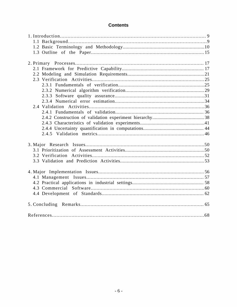
Contents
1. Introduction................................................................................................. 91.1 Background............................................................................................91.2 Basic Terminology and Methodology.............................................................101.3 Outline of the Paper................................................................................. 15
2. Primary Processes........................................................................................ 172.1 Framework for Predictive Capability............................................................. 172.2 Modeling and Simulation Requirements..........................................................212.3 Verification Activities............................................................................... 25
2.4 Validation Activities.................................................................................362.4.1 Fundamentals of validation................................................................. 362.4.2 Construction of validation experiment hierarchy......................................... 382.4.3 Characteristics of validation experiments..................................................412.4.4 Uncertainty quantification in computations............................................... 442.4.5 Validation metrics............................................................................ 46
3. Major Research Issues....................................................................................503.1 Prioritization of Assessment Activities............................................................503.2 Verification Activities............................................................................... 523.3 Validation and Prediction Activities............................................................... 53
4. Major Implementation Issues............................................................................ 564.1 Management Issues................................................................................. 574.2 Practical applications in industrial settings....................................................... 584.3 Commercial Software...............................................................................604.4 Development of Standards......................................................................... 62
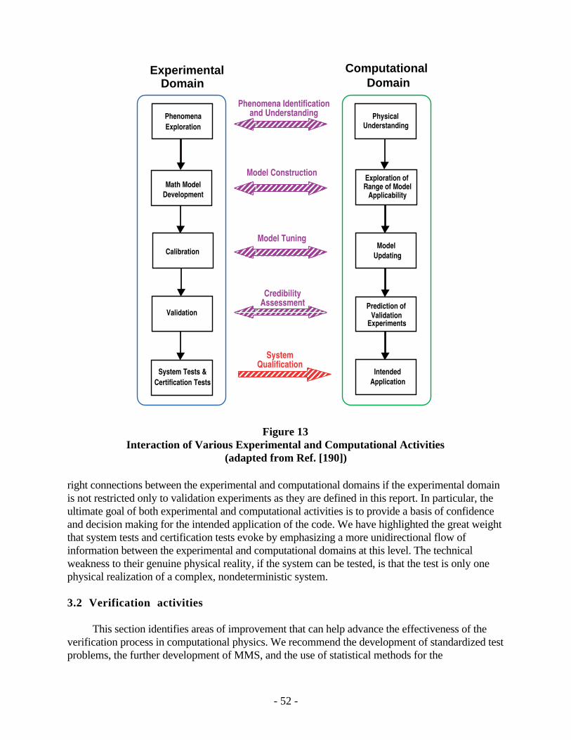
1 Phases of Modeling and Simulation and the Role of V&V................................ 122 Verification Process............................................................................ 143 Validation Process.............................................................................. 154 Relationship of Validation to Prediction......................................................185 Possible Relationships of the Validation Domain to the Application Domain............196 Verification-Validation-Predictive Process...................................................237 Aspects of PIRT Related to Application Requirements.....................................248 Integrated View of Code Verification in Computational Physics..........................289 Typical Relationship Between the Application Domain and the Validation Domain.... 3710 Validation Hierarchy for a Hypersonic Cruise Missile..................................... 4011 Validation Pyramid for a Hypersonic Cruise Missile.......................................4112 Increasing Quality of Validation Metrics..................................................... 4813 Interaction of Various Experimental and Computational Activities....................... 52
- 7 -
Acronyms and Abbreviations
AC Application ChallengesAIAA American Institute of Aeronautics and AstronauticsASME American Society of Mechanical EngineersASCI Accelerated Strategic Computing InitiativeCFD computational fluid dynamicsDMSO Defense Modeling and Simulation OfficeDoD Department of DefenseDOE Department of EnergyERCOFTAC European Research Community On Flow, Turbulence, And CombustionGCI Grid Convergence IndexGNC guidance, navigation and controlIEEE Institute of Electrical and Electronics EngineersMMS Method of Manufactured SolutionsNAFEMS National Agency for Finite Element Methods and StandardsNIST National Institute of Standards and TechnologyNPARC National Project for Applications-oriented Research in CFDPDE partial differential equationPIRT Phenomena Identification and Ranking TableQ-NET-CFD Thematic Network on Quality and Trust for the Industrial Applications of CFDSCS Society for Computer SimulationSQA software quality assuranceSQE software quality engineeringODE ordinary differential equationOR operations researchV&V verification and validation
- 8 -
1. Introduction
1.1 Background
During the last three or four decades, computer simulations of physical processes have beenincreasingly used in scientific research and in the analysis and design of engineered systems. Thesystems of interest have been existing or proposed systems that operate, for example, at designconditions, off-design conditions, and failure-mode conditions in accident scenarios. The systemsof interest have also been natural systems, for example, computer simulations for environmentalimpact, as in the analysis of surface-water quality and the risk assessment of underground nuclear-waste repositories. These kinds of predictions are beneficial in the development of public policy,the preparation of safety procedures, and the determination of legal liability. Thus, because of theimpact that modeling and simulation predictions can have, the credibility of the computationalresults is of great concern to engineering designers and managers, public officials, and those whoare affected by the decisions that are based on these predictions.
For engineered systems, terminology such as “virtual prototyping” and “virtual testing” isnow being used in engineering development to describe numerical simulation for the design,evaluation, and “testing” of new hardware and even entire systems. This new trend of modelingand simulation-based design is primarily driven by increased competition in many markets, e.g.,aircraft, automobiles, propulsion systems, and consumer products, where the need to decrease thetime and cost of bringing products to market is intense. This new trend is also driven by the highcost and time that are required for testing laboratory or field components as well as completesystems. Furthermore, the safety aspects of the product or system represent an important,sometimes dominant, element of testing or validating numerical simulations. The potential legal andliability costs of hardware failures can be staggering to a company, the environment, or the public.This consideration is especially critical, given that we may be interested in the reliability,robustness, or safety of high-consequence systems that cannot ever be physically tested. Examplesare the catastrophic failure of a full-scale containment building for a nuclear power plant, a firespreading through (or explosive damage to) a high-rise office building, ballistic missile defensesystems, and a nuclear weapon involved in a transportation accident. In contrast, however, aninaccurate or misleading numerical simulation for a scientific research project has comparatively noimpact.
Users and developers of computational simulations today face a critical question: Howshould confidence in modeling and simulation be critically assessed? Verification and validation(V&V) of computational simulations are the primary methods for building and quantifying thisconfidence. Briefly, verification is the assessment of the accuracy of the solution to acomputational model by comparison with known solutions. Validation is the assessment of theaccuracy of a computational simulation by comparison with experimental data. In verification, therelationship of the simulation to the real world is not an issue. In validation, the relationshipbetween computation and the real world, i.e., experimental data, is the issue.
In the United States, the Defense Modeling and Simulation Office (DMSO) of the Departmentof Defense (DoD) has been the leader in the development of fundamental concepts and terminologyfor V&V.[48,50] In the past five years, the Accelerated Strategic Computing Initiative (ASCI) ofthe Department of Energy (DOE) has also taken a strong interest in V&V. The ASCI program isfocused on computational physics and computational mechanics, whereas the DMSO hastraditionally emphasized high-level systems engineering, such as ballistic missile defense systems,
- 9 -
warfare modeling, and simulation-based system acquisition. Of the work conducted by DMSO,Cohen, et al. recently observed:[34] “Given the critical importance of model validation . . . , it issurprising that the constituent parts are not provided in the (DoD) directive concerning . . .validation. A statistical perspective is almost entirely missing in these directives.” We believe thisobservation properly reflects the state of the art in V&V, not just the directives of DMSO. That is,the state of the art has not developed to the place where one can clearly point out all of the actualmethods, procedures, and process steps that must be undertaken for V&V.
It is fair to say that computationalists (code users and code developers) and experimentalistsin the field of fluid dynamics have been pioneers in the development of methodology andprocedures in validation. However, it is also fair to say that the field of computational fluiddynamics (CFD) has, in general, proceeded along a path that is largely independent of validation.There are diverse reasons why the CFD community has not perceived a strong need for code V&V,especially validation. One reason is that a competitive and frequently adversarial relationship (atleast in the United States) has often existed between computationalists and experimentalists,resulting in a lack of cooperation between the two groups. We, on the other hand, viewcomputational simulation and experimental investigations as complementary and synergistic. Tothose who might say, “Isn’t that obvious?” we would answer, “It should be, but they have notalways been viewed as complementary.” In retrospect, the relationship between computationalistsand experimentalists is probably understandable because it represents the classic case of a newtechnology (computational simulation) that is rapidly growing and attracting a great deal ofvisibility and funding support that had been in the domain of the older technology(experimentation).
It is our view that the field of structural dynamics has enjoyed, in general, a more beneficialand synergistic relationship between computationalists and experimentalists. We believe this typeof relationship has developed because of the strong dependence of structural dynamics models onexperimental measurements. Most researchers in the field of structural dynamics have referred tothis interaction as “model validation.” As discussed in Section 2.1, we believe a more precise termfor this interaction is either “model updating” or “model calibration.” That is, the primaryinteraction between computation and experiment is to update or “tune” the unknown parameters inthe computational model using the experimental results from modal testing. This approach instructural dynamics has proven to be very effective because it permits the estimation of specificconstituents of poorly known physics in the computational models. In structural dynamics theproblem primarily arises in poor understanding of the localized deformation of connectors andjoints between structural elements in the computational models. A similar approach is used in fluiddynamics when dealing with turbulent reacting flows and two-phase flows.
From a historical perspective, the operations research (OR) and systems engineeringcommunities have provided the philosophical foundations for verification and validation. With therecent interest in V&V from the CFD and computational physics communities, one recognizessignificant differences in perspectives between the historical view and the view held by thecomputational physics community. (For simplicity, we will refer to all fields of computationalengineering and physics, e.g., CFD, computational solid mechanics, structural dynamics, shockwave physics, computational chemistry, etc., as computational physics.)
1.2 Basic Terminology and Methodology
There is a wide variety of different meanings used for V&V in the various technicaldisciplines. For example, the meanings used by the Institute of Electrical and Electronics Engineers
- 10 -
(IEEE) and the software quality assurance community are different from the meanings used in theDoD modeling and simulation community. And given that members of the different technicalcommunities often work together on V&V activities, we expect there will be long-term ambiguityand confusion resulting from terminology differences. Although we have not reviewed all of thedifferent meanings in this paper, we refer the reader to references that describe the varyingusage.[3,7,49,50,97-99] For reviews of the historical development of the terminology forverification, validation, and prediction see, for example, Refs. [139,147,148].
The DMSO under the DoD has played a major role in attempting to standardize the definitionsof V&V. In 1994 the DoD published definitions of V&V that are clear, concise, and directly usefulby themselves.[48-50] From the perspective of the computational engineering and physicscommunities, however, the definition of verification by the DoD does not make it clear that theaccuracy of the numerical solution to the partial differential equations (PDEs) should be included inthe definition. To clarify this issue, the CFD Committee on Standards of the American Institute ofAeronautics and Astronautics (AIAA) proposed a slight modification to the DoD definition. Thispaper will use the DoD definitions, with the AIAA modification for verification.[3]
Verification: The process of determining that a model implementation accurately represents thedeveloper's conceptual description of the model and the solution to the model.
Validation: The process of determining the degree to which a model is an accuraterepresentation of the real world from the perspective of the intended uses of the model.
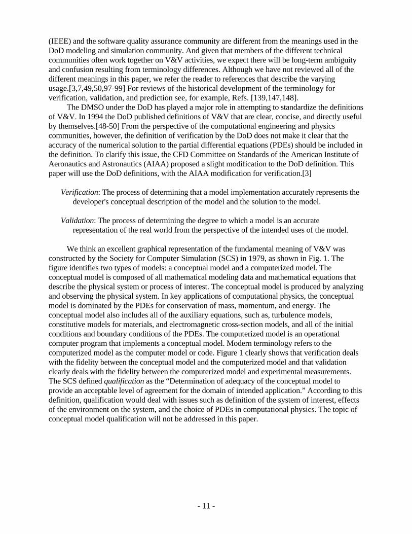
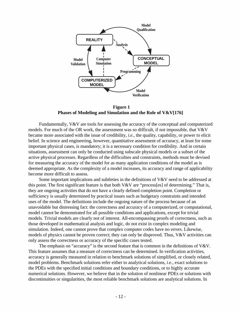
We think an excellent graphical representation of the fundamental meaning of V&V wasconstructed by the Society for Computer Simulation (SCS) in 1979, as shown in Fig. 1. Thefigure identifies two types of models: a conceptual model and a computerized model. Theconceptual model is composed of all mathematical modeling data and mathematical equations thatdescribe the physical system or process of interest. The conceptual model is produced by analyzingand observing the physical system. In key applications of computational physics, the conceptualmodel is dominated by the PDEs for conservation of mass, momentum, and energy. Theconceptual model also includes all of the auxiliary equations, such as, turbulence models,constitutive models for materials, and electromagnetic cross-section models, and all of the initialconditions and boundary conditions of the PDEs. The computerized model is an operationalcomputer program that implements a conceptual model. Modern terminology refers to thecomputerized model as the computer model or code. Figure 1 clearly shows that verification dealswith the fidelity between the conceptual model and the computerized model and that validationclearly deals with the fidelity between the computerized model and experimental measurements.The SCS defined qualification as the “Determination of adequacy of the conceptual model toprovide an acceptable level of agreement for the domain of intended application.” According to thisdefinition, qualification would deal with issues such as definition of the system of interest, effectsof the environment on the system, and the choice of PDEs in computational physics. The topic ofconceptual model qualification will not be addressed in this paper.
- 11 -
ModelVerification
ModelQualification
ModelValidation
Analysis
ComputerSimulation
Programming
COMPUTERIZEDMODEL
REALITY
CONCEPTUALMODEL
Figure 1Phases of Modeling and Simulation and the Role of V&V[176]
Fundamentally, V&V are tools for assessing the accuracy of the conceptual and computerizedmodels. For much of the OR work, the assessment was so difficult, if not impossible, that V&Vbecame more associated with the issue of credibility, i.e., the quality, capability, or power to elicitbelief. In science and engineering, however, quantitative assessment of accuracy, at least for someimportant physical cases, is mandatory; it is a necessary condition for credibility. And in certainsituations, assessment can only be conducted using subscale physical models or a subset of theactive physical processes. Regardless of the difficulties and constraints, methods must be devisedfor measuring the accuracy of the model for as many application conditions of the model as isdeemed appropriate. As the complexity of a model increases, its accuracy and range of applicabilitybecome more difficult to assess.
Some important implications and subtleties in the definitions of V&V need to be addressed atthis point. The first significant feature is that both V&V are “process[es] of determining.” That is,they are ongoing activities that do not have a clearly defined completion point. Completion orsufficiency is usually determined by practical issues such as budgetary constraints and intendeduses of the model. The definitions include the ongoing nature of the process because of anunavoidable but distressing fact: the correctness and accuracy of a computerized, or computational,model cannot be demonstrated for all possible conditions and applications, except for trivialmodels. Trivial models are clearly not of interest. All-encompassing proofs of correctness, such asthose developed in mathematical analysis and logic, do not exist in complex modeling andsimulation. Indeed, one cannot prove that complex computer codes have no errors. Likewise,models of physics cannot be proven correct; they can only be disproved. Thus, V&V activities canonly assess the correctness or accuracy of the specific cases tested.
The emphasis on “accuracy” is the second feature that is common in the definitions of V&V.This feature assumes that a measure of correctness can be determined. In verification activities,accuracy is generally measured in relation to benchmark solutions of simplified, or closely related,model problems. Benchmark solutions refer either to analytical solutions, i.e., exact solutions tothe PDEs with the specified initial conditions and boundary conditions, or to highly accuratenumerical solutions. However, we believe that in the solution of nonlinear PDEs or solutions withdiscontinuities or singularities, the most reliable benchmark solutions are analytical solutions. In
- 12 -
validation activities, accuracy is measured in relation to experimental data, i.e., our best indicationof reality. Since all experimental data have random (statistical) and bias (systematic) errors, theissue of “correctness,” in an absolute sense, becomes impossible. From an engineeringperspective, however, we do not require “absolute truth”: we only expect a statistically meaningfulcomparison of computational results and experimental measurements. These issues are discussedin more detail in Section 2.4.
Effectively, verification provides evidence (substantiation) that the conceptual (continuummathematics) model is solved correctly by the discrete-mathematics computer code. (Note: Whenwe refer to “continuum mathematics,” we are not referring to the physics being modeled by themathematics. For example, the equations for noncontinuum fluid dynamics are commonlyexpressed with continuum mathematics.) Verification does not address whether the conceptualmodel has any relationship to the real world. Validation, on the other hand, provides evidence(substantiation) for how accurately the computational model simulates reality. This perspectiveimplies that the model is solved accurately. However, multiple errors or inaccuracies can cancelone another and give the appearance of a validated solution. Verification, thus, is the first step ofthe validation process and, while not simple, is much less involved than the more complexstatistical nature of validation. Validation addresses the question of the fidelity of the model tospecific conditions of the real world. As Roache[165] succinctly states, “Verification deals withmathematics; validation deals with physics.”
As a final comment on terminology, it is our view that the DoD definition of validation doesnot include the concept of adequacy of the computational result for the intended uses of themodel. Stated differently, we argue that validation is the process of determining the degree towhich computational simulation results agree with experimental data. We recognize that thisinterpretation of the meaning of validation is narrower than the interpretation that is widely acceptedin the DoD community. It is our understanding that the DoD community considers validation to bethe process of determining the degree to which the computational model results are adequate forthe application of interest. This important topic of divergent interpretations of validation is brieflydiscussed in recommendations for future work, Section 4.4. Regardless of whether the readeragrees with our interpretation, we have chosen to clarify our view now to help avoid confusionthroughout the paper. Stating our view succinctly: validation deals with quantified comparisonsbetween experimental data and computational data; not the adequacy of the comparisons.
In 1998 the Computational Fluid Dynamics Committee on Standards of the AIAA contributedto the basic methodology and procedures for V&V.[3] The Guide for the Verification andValidation of Computational Fluid Dynamics Simulations, referred to herein as the “AIAAGuide,” was the first engineering standards document that addressed issues of particular concern tothe computational physics community. In the following paragraphs we have briefly summarizedthe basic methodology for V&V from the AIAA Guide.
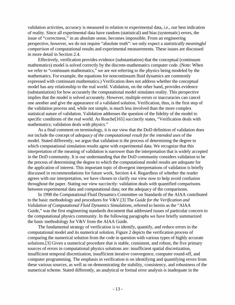
The fundamental strategy of verification is to identify, quantify, and reduce errors in thecomputational model and its numerical solution. Figure 2 depicts the verification process ofcomparing the numerical solution from the code in question with various types of highly accuratesolutions.[3] Given a numerical procedure that is stable, consistent, and robust, the five primarysources of errors in computational physics solutions are: insufficient spatial discretization,insufficient temporal discretization, insufficient iterative convergence, computer round-off, andcomputer programming. The emphasis in verification is on identifying and quantifying errors fromthese various sources, as well as on demonstrating the stability, consistency, and robustness of thenumerical scheme. Stated differently, an analytical or formal error analysis is inadequate in the
- 13 -
verification process; verification relies on demonstration and quantification of numericalaccuracy. Note that the recommended methodology presented here applies to finite-difference,finite-volume, finite-element, and boundary-element discretization procedures.
The first three error sources listed in the previous paragraph (spatial discretization, temporaldiscretization, and iterative procedure) are considered to be within the traditional realm ofcomputational physics and there is extensive literature dealing with each of these topics. The fourtherror source, computer round-off, is rarely dealt with in computational physics. Collectively, thesefour topics in verification could be referred to as solution verification or solution error assessment.The fifth error source, computer programming, is generally considered to be in the realm ofcomputer science or software engineering. Programming errors, which can occur, for example, ininput data files, source-code programming of the numerical algorithm, output data files, compilers,and operating systems, generally are addressed using methods and tools in software qualityassurance (SQA), also referred to as software quality engineering (SQE).[111] The identificationof programming errors is usually referred to as code verification, as opposed to solutionverification.[165,166] In our opinion, the perspectives and emphases of SQA and computationalphysics are sufficiently different and thus should be addressed separately: code verification, whichemphasizes the accuracy of the numerical algorithm that is used to solve the discrete form of thePDEs; and SQA, which emphasizes the issues in computer science. Each of these topics isdiscussed in Section 2.3.
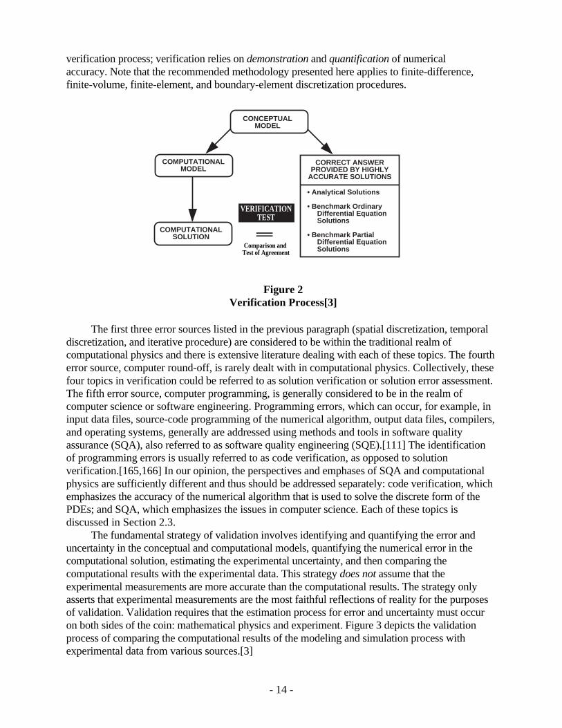
The fundamental strategy of validation involves identifying and quantifying the error anduncertainty in the conceptual and computational models, quantifying the numerical error in thecomputational solution, estimating the experimental uncertainty, and then comparing thecomputational results with the experimental data. This strategy does not assume that theexperimental measurements are more accurate than the computational results. The strategy onlyasserts that experimental measurements are the most faithful reflections of reality for the purposesof validation. Validation requires that the estimation process for error and uncertainty must occuron both sides of the coin: mathematical physics and experiment. Figure 3 depicts the validationprocess of comparing the computational results of the modeling and simulation process withexperimental data from various sources.[3]
- 14 -
COMPUTATIONALMODEL
=
VALIDATIONTEST
CORRECT ANSWERPROVIDED BY
EXPERIMENTAL DATA
• Unit Problems
• Benchmark Cases
• Subsystem Cases
• Complete SystemComparison and
Test of Agreement
COMPUTATIONALSOLUTION
CONCEPTUALMODEL
REALWORLD
Figure 3Validation Process[3]
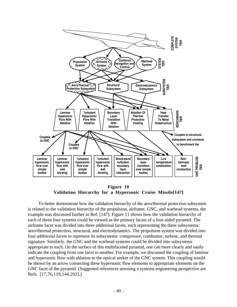
Because of the infeasibility and impracticality of conducting true validation experiments onmost complex or large scale systems, the recommended method is to use a building-blockapproach.[3,37,125,128,179,180] This approach divides the complex engineering system ofinterest into at least three progressively simpler tiers: subsystem cases, benchmark cases, and unitproblems. The strategy in the tiered approach is to assess how accurately the computational resultscompare with the experimental data (with quantified uncertainty estimates) at multiple degrees ofphysics coupling and geometric complexity. The approach is clearly constructive in that it (1)recognizes that there is a hierarchy of complexity in systems and simulations and (2) recognizesthat the quantity and accuracy of information that is obtained from experiments vary radically overthe range of tiers. Furthermore, this approach demonstrates that validation experiments can beconducted at many different levels of physics and system complexity. Each comparison ofcomputational results with experimental data allows an inference of validation concerning tiers bothabove and below the tier where the comparison is made. However, the quality of the inferencedepends greatly on the complexity of the tiers above and below the comparison tier. For simplephysics, the inference may be very strong, e.g., laminar, single phase, Newtonian, nonreactingflow, and rigid-body structural dynamics. However, for complex physics, the inference iscommonly very weak, e.g., turbulent reacting flow and fracture dynamics. This directly reflectsthe quality of our scientific knowledge about the experiments and calculations that are beingcompared for more complex tiers.
1.3 Outline of the Paper
This paper presents our viewpoint on the state of the art in V&V in computational physics.We have not attempted herein to provide a comprehensive review of the multitudinouscontributions to V&V from many diverse fields. This literature represents distinctively different
- 15 -
perspectives and approaches, ranging from engineering and physics to operations research. Recentreviews of the literature are given in Refs. [14,108,109,134,148,165,168,202]. Recent workproviding wide-ranging procedures in V&V is described in Refs. [26,148,159,190]. We haveattempted in this paper to bring together many different perspectives on V&V, highlight thoseperspectives that are effective from a practical engineering viewpoint, suggest future researchtopics, and discuss key implementation issues that are necessary to improve the effectiveness ofV&V. Our views about the research needs and management issues in V&V are very practical: Whatmethods and techniques need to be developed and what changes in the views of management needto occur to increase the usefulness, reliability, and impact of computational physics for decisionmaking about engineering systems?
Section 2 describes the primary processes in V&V and the relationship of V&V to predictivecapability. V&V are the key building blocks in assessing the confidence in the predictive capabilityof a computational physics code. The section begins with a description of the framework in whichpredictive capability relies on V&V, as well as other factors that affect predictive capability. Wealso briefly discuss how this framework is related to more traditional approaches of predictivecapability, e.g., Bayesian estimation. The importance of requirements for a computational-physicscapability is stressed so that effective and efficient V&V activities can be conducted. Following theframework discussion, we present a summary of verification activities, emphasizing codeverification, SQA, and numerical error estimation. A discussion of validation activities follows,highlighting methods for focusing on the validation experiments most important to the predictivecapability required. The section concludes with a discussion of hierarchical experiments forvalidation, characteristics of validation experiments, the need to perform nondeterministicsimulations in comparisons with experimental data, and validation metrics.
Section 3 discusses the research issues that we believe must be addressed for V&V to bemore effective in improving confidence in computational predictive capability. We begin with adiscussion of methods for prioritizing V&V assessment activities. Needed research in verificationactivities, such as, statistical methods for code verification and the method of manufacturedsolutions, are discussed. Topics discussed with regard to validation research are: development anduse of hierarchical validation diagrams; and the construction and use of validation metricsincorporating statistical measures. We close the section with the difficult research issue of how toquantify uncertainty in predictive capability, given an arbitrary set of validation experiments, e.g.,how to estimate the uncertainty of a computational prediction when, in some sense, we areextrapolating beyond the validation database.
Section 4 discusses issues related to improving the implementation of V&V activities in arealistic engineering environment and a commercial software environment. These issues includeneeded improvements in management of verification activities, the key role of analysts and decisionmakers as code customers, and obstacles to the improved effectiveness of V&V. Examples ofobstacles are the conflicting perspectives of code developers, analysts, hardware designers, andexperimentalists; competition between organizations and nations; and the loss of focus on the needsof the customer for computational physics analyses. Also discussed are the effects of cost andschedule constraints on practical applications in industrial settings, the demands of customers oncommercial software companies, and the large-scale validation database activity underway inEurope.
Section 5 presents some closing remarks concerning the status of V&V and the need forimprovement.
- 16 -
2. Primary Processes
2.1 Framework for Predictive Capability
The issues underlying the V&V of mathematical and computational models of physicalsystems, including those systems with strong human interaction, touch on the very foundations ofmathematics, science, and human behavior. Verification is rooted in issues pertaining to continuumand discrete mathematics and to the accuracy and correctness of complex logical structures(computer codes). Validation is deeply rooted in the question of how formal constructs(mathematical models) of nature and human behavior can be tested by physical observation. In theOR field, the systems being analyzed can be extraordinarily complex, such as, industrial planningmodels, marketing models, national and world economic models, monetary investment models,and military conflict models. For these types of situations, one must deal with statistical modelswhere statistical calibration and parameter estimation are crucial elements in building the models.These complex models commonly involve a strong coupling of complex physical processes,human behavior, and computer-controlled systems. For such complex systems and processes,fundamental conceptual issues immediately arise about how to assess the accuracy of the modeland the resulting simulations. Indeed, the predictive accuracy of most of these models cannot beassessed in any meaningful way, except for predictive cases that are very near, in some sense, thecalibration database.
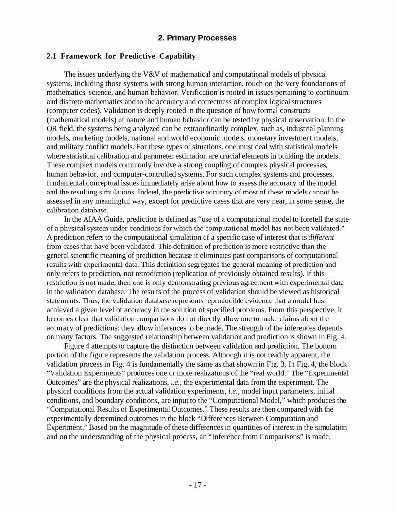
In the AIAA Guide, prediction is defined as “use of a computational model to foretell the stateof a physical system under conditions for which the computational model has not been validated.”A prediction refers to the computational simulation of a specific case of interest that is differentfrom cases that have been validated. This definition of prediction is more restrictive than thegeneral scientific meaning of prediction because it eliminates past comparisons of computationalresults with experimental data. This definition segregates the general meaning of prediction andonly refers to prediction, not retrodiction (replication of previously obtained results). If thisrestriction is not made, then one is only demonstrating previous agreement with experimental datain the validation database. The results of the process of validation should be viewed as historicalstatements. Thus, the validation database represents reproducible evidence that a model hasachieved a given level of accuracy in the solution of specified problems. From this perspective, itbecomes clear that validation comparisons do not directly allow one to make claims about theaccuracy of predictions: they allow inferences to be made. The strength of the inferences dependson many factors. The suggested relationship between validation and prediction is shown in Fig. 4.
Figure 4 attempts to capture the distinction between validation and prediction. The bottomportion of the figure represents the validation process. Although it is not readily apparent, thevalidation process in Fig. 4 is fundamentally the same as that shown in Fig. 3. In Fig. 4, the block“Validation Experiments” produces one or more realizations of the “real world.” The “ExperimentalOutcomes” are the physical realizations, i.e., the experimental data from the experiment. Thephysical conditions from the actual validation experiments, i.e., model input parameters, initialconditions, and boundary conditions, are input to the “Computational Model,” which produces the“Computational Results of Experimental Outcomes.” These results are then compared with theexperimentally determined outcomes in the block “Differences Between Computation andExperiment.” Based on the magnitude of these differences in quantities of interest in the simulationand on the understanding of the physical process, an “Inference from Comparisons” is made.
- 17 -
Complex System(not in validation
database)
ComputationalModel
Computational Resultsof Experimental
Outcomes
Experimental Outcomes
ValidationExperiments
DifferencesBetween Computation
and Experiment
InferenceFrom
Comparisons
Computational Predictionsof Complex System
Outcomes
P R E D I C T I O N
V A L I D A T I O N
Figure 4Relationship of Validation to Prediction[57,148]
The upper portion of Fig. 4 represents the prediction process. The “Complex System” ofinterest should drive the entire modeling and simulation process, but most of the realizations ofinterest, i.e., predictions, are not in the validation database. That is, when a physical realization isconducted as part of the validation database, regardless of the tier as discussed in Section 2.4.2,the realization becomes part of the “Validation Experiments.” Predictions for conditions of interestare made using the “Computational Model,” resulting in “Computational Predictions of ComplexSystem Outcomes.” The confidence in these predictions is determined by the “Inference fromComparisons” and the level of understanding of the physical process.
The process of logical inference of accuracy of a computational model stemming from itsassociated validation database is analogous to similar processes and conclusions for classicalscientific theories. However, we argue that the strength or confidence in the inference fromcomputational simulation is, and should be, much weaker than traditional scientific theories.Computational simulation relies on the same logic as traditional science, but it also relies on manyadditional mathematical issues, e.g., discretization algorithms and grid quality, and practicalimplementation issues, e.g., computer hardware, operating-system software, source-codereliability, and analyst skill, that are not present in classical scientific theories. (In this paper“analyst” refers to the individual, or group of individuals, who constructs the computationalmodel, including all physical and numerical inputs to the model, and then uses the computer codeto produce a simulation.) One of the key theoretical issues is the state of knowledge of the processbeing modeled. Zeigler, et al.[202] gives a detailed discussion of hierarchical levels of knowledgeof a system. For physical processes that are well understood both physically and mathematically,the inference can be quite strong. For complex physical processes, the inference can be quite weak.A general mathematical method for determining how the value and consequence of such aninference degrades as the physical process becomes more complex has not been formulated. Forexample, in a complex physical process how do you determine “how nearby” the prediction case isfrom cases in the validation database? This is a topological question applied to an ill-defined space.Struggling with the strength or quantification of the inference in a prediction is, and will remain, an
- 18 -
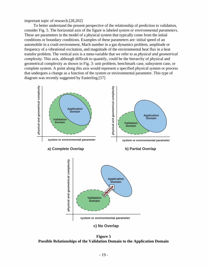
important topic of research.[28,202]To better understand the present perspective of the relationship of prediction to validation,
consider Fig. 5. The horizontal axis of the figure is labeled system or environmental parameters.These are parameters in the model of a physical system that typically come from the initialconditions or boundary conditions. Examples of these parameters are: initial speed of anautomobile in a crash environment, Mach number in a gas dynamics problem, amplitude orfrequency of a vibrational excitation, and magnitude of the environmental heat flux in a heattransfer problem. The vertical axis is a meta-variable that we refer to as physical and geometricalcomplexity. This axis, although difficult to quantify, could be the hierarchy of physical andgeometrical complexity as shown in Fig. 3: unit problem, benchmark case, subsystem case, orcomplete system. A point along this axis would represent a specified physical system or processthat undergoes a change as a function of the system or environmental parameter. This type ofdiagram was recently suggested by Easterling.[57]
ValidationDomain
b) Partial Overlapa) Complete Overlap
ValidationDomain
ApplicationDomain
ApplicationDomain
system or environmental parameter system or environmental parameter
ph
ysic
al a
nd
geo
met
rica
l co
mp
lexi
ty
ph
ysic
al a
nd
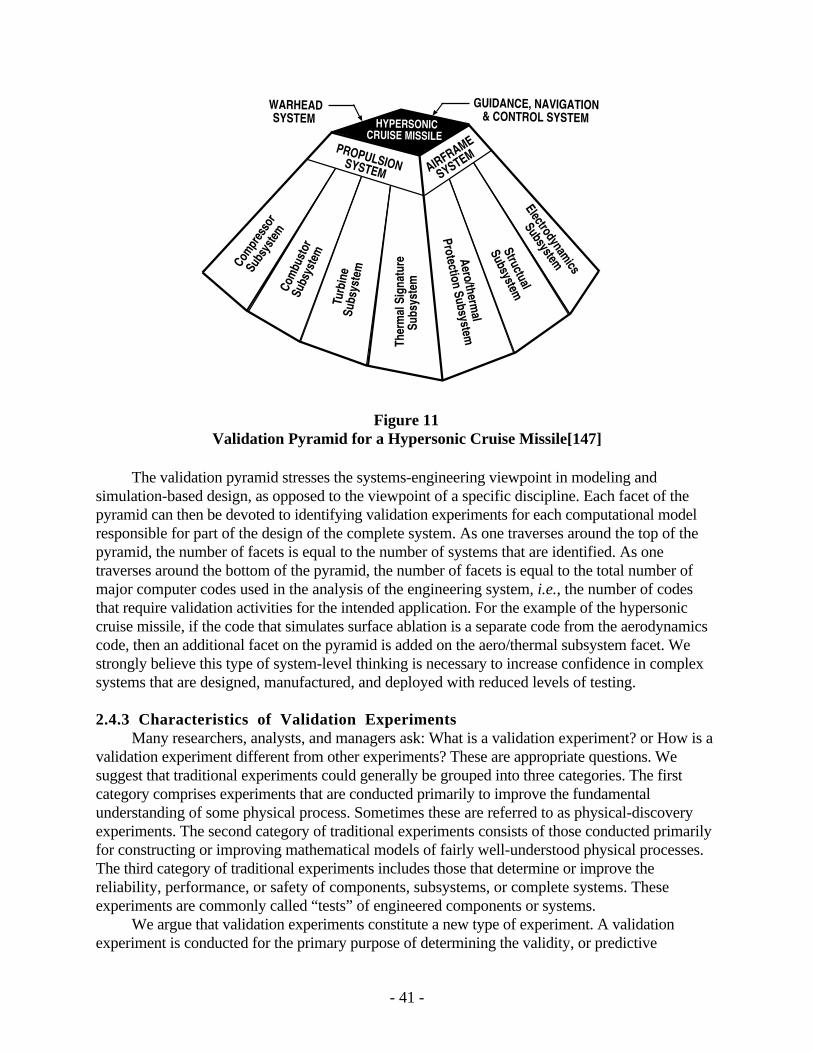
geo
met
rica
l co
mp
lexi
ty
ApplicationDomain
ValidationDomain
c) No Overlap
system or environmental parameter
ph
ysic
al a
nd
geo
met
rica
l co
mp
lexi
ty
Figure 5Possible Relationships of the Validation Domain to the Application Domain
- 19 -
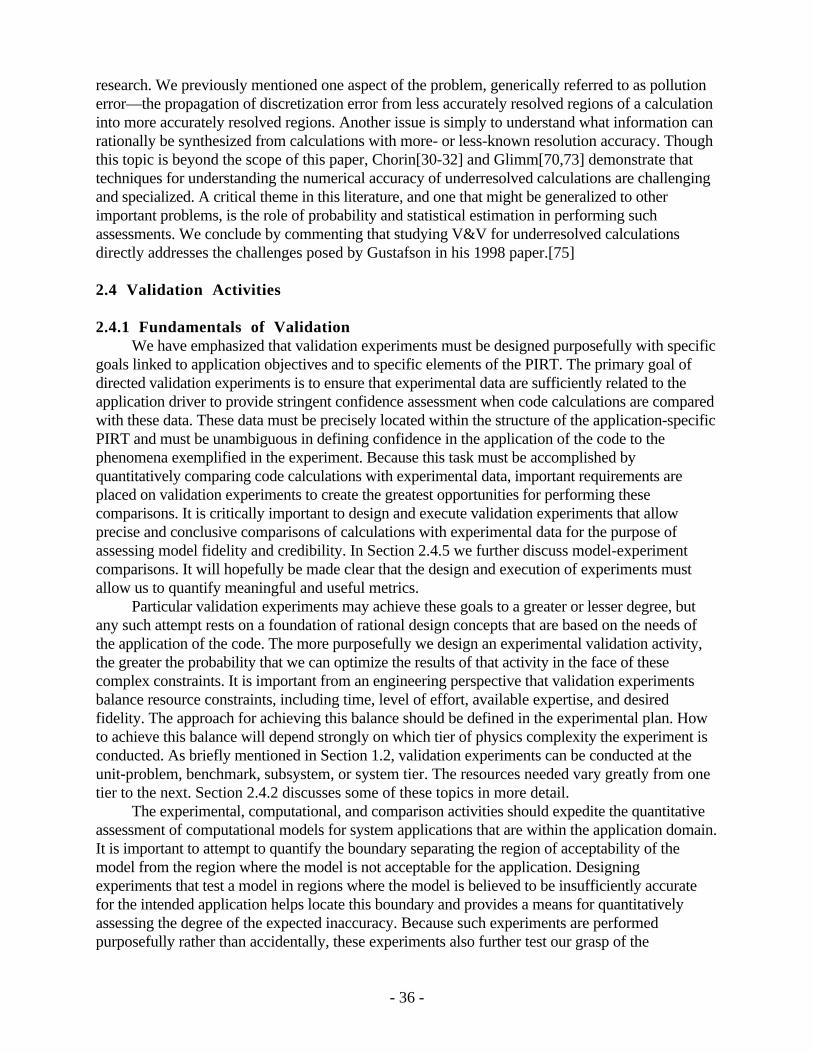
The “validation domain” in Fig. 5 suggests three features. First, in this region we have highconfidence that the relevant physics is understood and modeled at a level that is commensurate withthe needs of the application. Second, this confidence has been quantitatively demonstrated bysatisfactory agreement between computations and experiments in the validation database for somerange of applicable parameters in the model. And third, the boundary of the domain indicates thatoutside this region there is a degradation in confidence in the quantitative predictive capability ofthe model. Stated differently, outside the validation domain the model may be credible, but itsquantitative capability has not been demonstrated. The “application domain” indicates the regionwhere predictive capability is needed from the model for the applications of interest.
Figure 5a depicts the prevalent situation in engineering, that is, the complete overlap of thevalidation domain with the application domain. The vast majority of modern engineering systemdesign is represented in Fig. 5a. Figure 5b represents the occasional engineering situation wherethere is significant overlap between the validation domain and the application domain. Someexamples are: the prediction of crash response of new automobile structures, entry of spacecraftprobes into the atmosphere of another planet, and the structural response of new designs for deep-water offshore oil platforms. Figure 5c depicts the situation where there is no overlap between thevalidation domain and the application domain. We believe that predictions for many high-consequence systems are in this realm because we are not able to perform experiments for closelyrelated conditions. We believe that the inference from the validation domain suggested in Fig. 5ccan only be made using both physics-based models and statistical methods. The need to performthis extrapolation reinforces our need for models to be judged on the basis of achieving the rightanswers for the right reasons in the validation regime. Model calibration, which employs explicittuning or updating of model parameters to achieve improved agreement with existing validationexperiments, does not fully assess uncertainty in the predictive use of the model. Stated morestrongly, it is not convincing that model calibration provides a starting point for the inferenceprocess demanded in Fig. 5c.
As a final conceptual issue concerning predictive capability, we strongly believe that a morecareful distinction between error and uncertainty is needed than has traditionally been made in thecomputational physics literature. We define error based on the AIAA Guide[3] (see also Refs.[144-146]) to be “A recognizable deficiency in any phase or activity of modeling and simulationsthat is not due to lack of knowledge.” This definition emphasizes the required feature that thedeficiency is identifiable or knowable upon examination, that is, the deficiency is notfundamentally caused by lack of knowledge. This definition leads to the so-called acknowledgedand unacknowledged errors. An acknowledged error is characterized by knowledge of divergencefrom an approach or ideal condition that is considered to be a baseline for accuracy. Examples ofacknowledged errors are finite precision arithmetic in a computer, approximations made to simplifythe modeling of a physical process, and conversion of PDEs into discrete equations. Anacknowledged error can therefore, in principle, be measured because its origins are fully identified.Solution verification, i.e., solution error estimation, deals with acknowledged errors. Forexample, we know that the discretization of the PDE and the approximate solution of the discreteequations introduce acknowledged errors. Unacknowledged errors are blunders or mistakes, suchas, programming errors, input data errors, and compiler errors. There are no straightforwardmethods for estimating, bounding, or ordering the contributions of unacknowledged errors. Codeverification and SQA activities primarily deal with unacknowledged errors, which is anotherimportant reason these activities are essential.
- 20 -
In a technical sense, the term uncertainty seems to have two rather different meanings. Thefirst meaning of uncertainty has its roots in probability and statistics: the estimated amount orpercentage by which an observed or calculated value may differ from the true value. This meaningof uncertainty has proven its usefulness over many decades, particularly in the estimation ofrandom uncertainty in experimental measurements.[35] The second meaning of uncertainty relatesto lack of knowledge about physical systems, particularly in the prediction of future events and theestimation of system reliability. The probabilistic-risk and safety assessment communities, as wellas the reliability engineering community, use the term epistemic uncertainty in this latter sense.The risk assessment community[39,63,65,85,95,155] refers to the former meaning, randomuncertainty, as aleatory uncertainty, as does the information theory community.[6,54,110,113,114,183]
Aleatory uncertainty is used to describe the inherent variation associated with the physicalsystem or environment being considered. Sources of aleatory uncertainty can commonly be singledout from other contributors to uncertainty by their representation as randomly distributed quantitiesthat can take on values in an established or known range, but for which the exact value will vary bychance from unit to unit or from time to time. The mathematical representation most commonlyused to characterize aleatory uncertainty is a probability distribution. Aleatory uncertainty is alsoreferred to in the literature as variability, irreducible uncertainty, inherent uncertainty, andstochastic uncertainty.
Epistemic uncertainty as a cause of nondeterministic behavior derives from some level ofignorance or lack of knowledge about the system or the environment. Thus, an increase inknowledge or information can lead to a reduction in the predicted uncertainty of the system’sresponse—all things being equal. Epistemic uncertainty can be introduced from a variety ofsources, such as, limited or nonexistent experimental data for a fixed (but unknown) physicalparameter, limited understanding of complex physical processes, or insufficient knowledgeconcerning initial conditions and boundary condition in an experiment. Epistemic uncertainty isalso referred to in the literature as reducible uncertainty, subjective uncertainty, and model formuncertainty.
Issues of acknowledged and unacknowledged errors are primarily discussed with regard toverification activities (Section 2.3). Issues of aleatory and epistemic uncertainty are primarilydiscussed with regard to validation and prediction capability activities (Sections 2.4 and 3.3).
Referring back to Fig. 5c, the requirement for use of a model “far from” the validationdatabase necessitates extrapolation well beyond the physical understanding gained strictly fromexperimental validation data. As a result, the type of uncertainty that dominates our inference to theapplication domain is epistemic uncertainty. For example, the modeling of specific types ofinteractions or coupling of physical processes may not have been validated together in the givenvalidation database. Examples of this situation are safety assessment of nuclear-reactors duringfailure conditions[103,115,131,137] and the assessment of nuclear-waste-repositoryperformance.[87,88,132,156] There is then significant epistemic uncertainty in the accuracy ofmodel predictions describing such interactions. Aleatory uncertainty will also be a factor in theinference, but the dominant contributor is lack of knowledge of the physical processes active in theextrapolation.
2.2 Modeling and Simulation Requirements
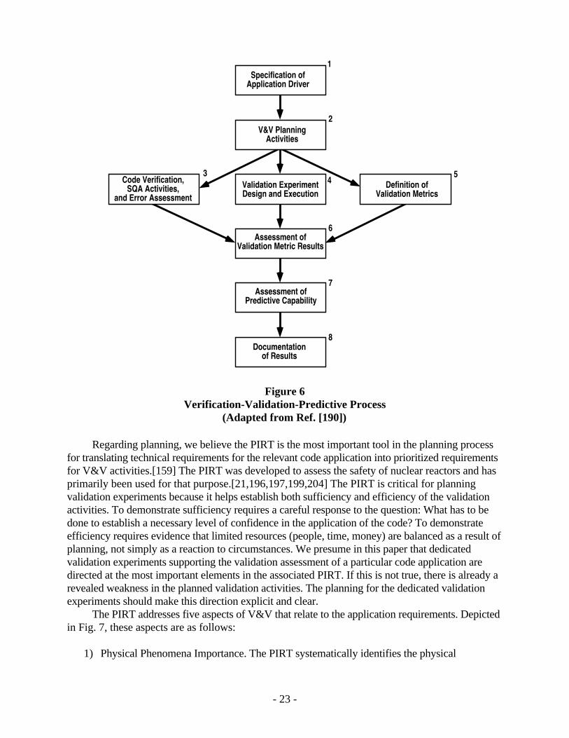
To improve the efficiency and confidence-building impact of V&V, we believe it is necessaryto improve the coupling of V&V activities with the requirements of the intended application of the
- 21 -
computational physics code. Figure 6 depicts a high-level view of the verification-validation-prediction process that begins with the specification of the application driver and the requirementsfor the computational physics code.[190] In Fig. 6 we suggest that the complete process reliesupon the following activities:
1. Identification and specification of the application driver that focuses the use of the codeunder discussion
2. Careful planning of V&V activities, especially the use of the Phenomena Identification andRanking Table (PIRT) to prioritize V&V activities for the application driver and preliminaryspecification of prediction accuracy requirements
3. Development, implementation, and documentation of code verification and SQA activitiesfor the code, as well as solution error assessment of validation calculations
4. Design and execution of validation experiment activities in accordance with the PIRT
5. Development and definition of appropriate metrics for comparing computational resultswith experimental results to measure confidence in the intended application of the code
6. Assessing the results of the validation metrics with regard to preliminary specification ofprediction accuracy requirements
7. Assessment of the predictive accuracy of the code using the validation metrics and therefined application requirements, with emphasis on high-level system response measures
8. Accurate and full documentation of the planning, results, and consequences of thevalidation activities, especially their implications for predictive confidence for theapplication driver of the code
Note that the although the activities shown in Fig. 6 are shown sequentially, the process istypically an iterative one.
This paper briefly discusses each of these eight activities, but Ref. [190] discusses each indetail. In this section we only comment on the two key activities that directly address the focus ofV&V on the requirements of the application: block 1 “Intended Application” and block 2“Planning.” The intended application is the application for which the modeling and simulationcapability is being developed. Concerning application requirements, validation activities mustassess confidence in the use of the code for a specified application. The application requirement atwhich a particular validation activity is directed is a critical planning element and must be definedbefore the performance of any specific validation work. One of the methods in risk assessment foridentifying specific applications deals with identifying system-application scenarios. In the nuclearweapons area, event scenarios are segregated into three wide categories to which the engineeringsystem might be subjected: normal, abnormal, and hostile environments. Although these categoriesmay not be appropriate for all engineering systems, we believe they are a helpful framework formany types of systems, e.g., systems ranging from military and commercial aircraft to spacecraftto power generation facilities and public buildings.
- 22 -
Specification ofApplication Driver
V&V PlanningActivities
Code Verification,SQA Activities,
and Error AssessmentValidation ExperimentDesign and Execution
Definition ofValidation Metrics
Assessment ofPredictive Capability
Documentationof Results
Assessment ofValidation Metric Results
1
2
34
5
6
7
8
Figure 6Verification-Validation-Predictive Process
(Adapted from Ref. [190])
Regarding planning, we believe the PIRT is the most important tool in the planning processfor translating technical requirements for the relevant code application into prioritized requirementsfor V&V activities.[159] The PIRT was developed to assess the safety of nuclear reactors and hasprimarily been used for that purpose.[21,196,197,199,204] The PIRT is critical for planningvalidation experiments because it helps establish both sufficiency and efficiency of the validationactivities. To demonstrate sufficiency requires a careful response to the question: What has to bedone to establish a necessary level of confidence in the application of the code? To demonstrateefficiency requires evidence that limited resources (people, time, money) are balanced as a result ofplanning, not simply as a reaction to circumstances. We presume in this paper that dedicatedvalidation experiments supporting the validation assessment of a particular code application aredirected at the most important elements in the associated PIRT. If this is not true, there is already arevealed weakness in the planned validation activities. The planning for the dedicated validationexperiments should make this direction explicit and clear.
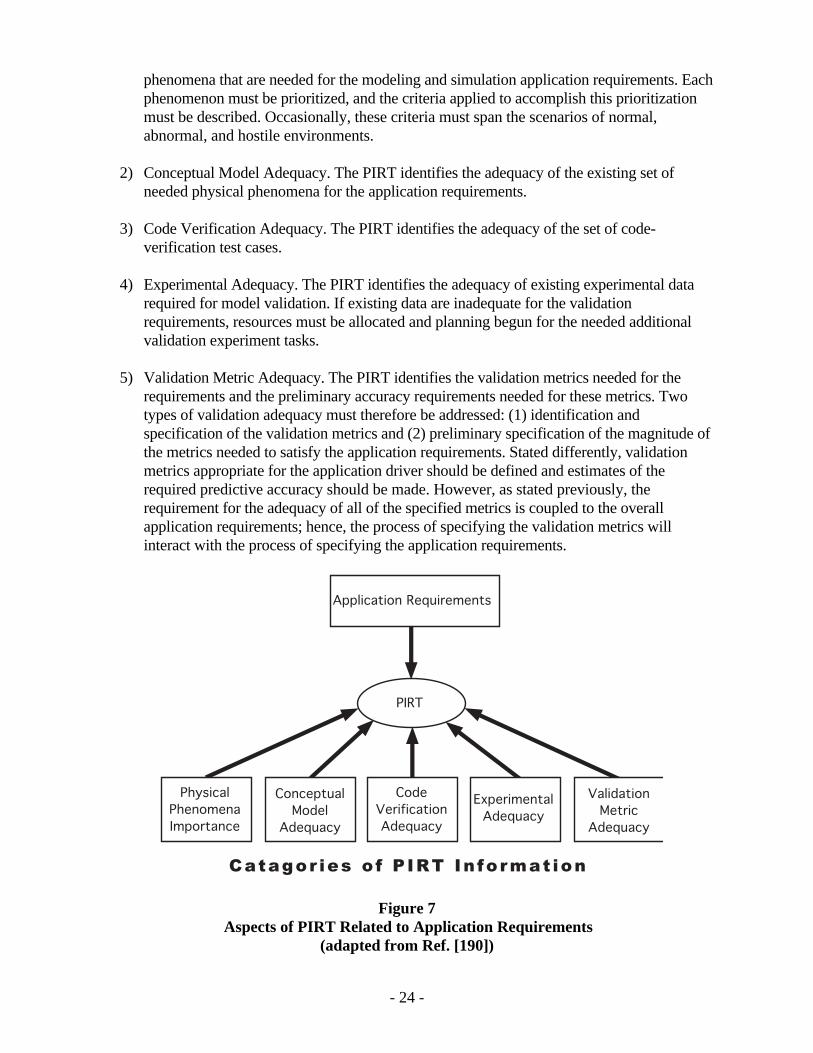
The PIRT addresses five aspects of V&V that relate to the application requirements. Depictedin Fig. 7, these aspects are as follows:
1) Physical Phenomena Importance. The PIRT systematically identifies the physical
- 23 -
phenomena that are needed for the modeling and simulation application requirements. Eachphenomenon must be prioritized, and the criteria applied to accomplish this prioritizationmust be described. Occasionally, these criteria must span the scenarios of normal,abnormal, and hostile environments.
2) Conceptual Model Adequacy. The PIRT identifies the adequacy of the existing set ofneeded physical phenomena for the application requirements.
3) Code Verification Adequacy. The PIRT identifies the adequacy of the set of code-verification test cases.
4) Experimental Adequacy. The PIRT identifies the adequacy of existing experimental datarequired for model validation. If existing data are inadequate for the validationrequirements, resources must be allocated and planning begun for the needed additionalvalidation experiment tasks.
5) Validation Metric Adequacy. The PIRT identifies the validation metrics needed for therequirements and the preliminary accuracy requirements needed for these metrics. Twotypes of validation adequacy must therefore be addressed: (1) identification andspecification of the validation metrics and (2) preliminary specification of the magnitude ofthe metrics needed to satisfy the application requirements. Stated differently, validationmetrics appropriate for the application driver should be defined and estimates of therequired predictive accuracy should be made. However, as stated previously, therequirement for the adequacy of all of the specified metrics is coupled to the overallapplication requirements; hence, the process of specifying the validation metrics willinteract with the process of specifying the application requirements.
������������ ��������
��������
�������
���������
���������
�����
��� ����
����
�����������
��� ����
�����������
��� ����
���������
������
��� ����
����
Catagor ies o f P IRT In format ion
Figure 7 Aspects of PIRT Related to Application Requirements
(adapted from Ref. [190])
- 24 -
As stressed by Boyack,[21] the PIRT is certainly not set in stone once it is formulated anddocumented. While a given formulation of the PIRT guides V&V activities, the PIRT must also beadaptable to reflect information gathered during the conduct of these activities. Importantly, to gainthe greatest advantage of its value during planning, the PIRT can and probably should be adaptedas experimental validation activities are conducted. Several different outcomes illustrate howexperimental validation activities can interact with and influence changes to the PIRT:
• A validation experiment may be planned and conducted under the assumption that a specificPIRT element has high importance. After the results of the experiment are analyzed, theimportance of that PIRT element is found to change from high to medium or low inresponse to these results. This does not argue that the underlying application requirementscould or would change as a result of experiments, only that the technical importance of anelement for validation may change.
• An experiment is conducted that reveals a shift of a PIRT element from low to highimportance. This may require, for example, that a subsequent exploratory experiment beperformed that was not identified in the existing PIRT.
• An experiment addressing a high-importance PIRT element is performed. The current codeimplementation addressing that phenomenon is believed to be adequate. However, it isdiscovered unexpectedly that the code cannot even function properly in defining theproposed experiments, thereby changing the ranking of the implementation to inadequate.
• An experiment designed to probe fully coupled phenomena reveals the presence of acompletely unexpected and unknown phenomenon that is of high importance for theapplication driver. Not only must the PIRT be changed to reflect this event, but also theoverall V&V effort for the code application may require significant revision. For example, apreviously low-ranked phenomenon may now be ranked high or a planned validationexperiment may have to be redefined as a phenomenon-exploration experiment.
• A validation experiment for a single phenomenon reveals that certain models implementedin the code must be recalibrated. This changes the code implementation from adequate toincomplete and may require additional planning for calibration experiments to improve thepre-calibration model capabilities.
2.3 Verification Activities
2.3.1 Fundamentals of VerificationTwo types of verification are generally recognized in computational modeling: code
verification and solution verification.[165,166] Because of recent work by severalinvestigators,[147,148] we now believe that code verification should be segregated into two parts:numerical algorithm verification and SQA. Numerical algorithm verification addresses the softwarereliability of the implementation of all of the numerical algorithms that affect the numerical accuracyand efficiency of the code. In other words, this verification process focuses on how correctly thenumerical algorithms are programmed (implemented) in the code and the accuracy and reliability of
- 25 -
the numerical algorithms themselves. This issue is of paramount importance in computationalphysics codes, whereas in conventional areas of application of SQA, such as, real-time controlsystems, this issue receives less emphasis. The major goal of numerical algorithm verification is toaccumulate sufficient evidence to demonstrate that the numerical algorithms in the code areimplemented correctly and functioning as intended. SQA emphasizes determining whether or notthe code, as a software system, is reliable (implemented correctly) and produces repeatable resultson specified computer hardware and a specified system with a specified software environment,including compilers, libraries, etc. SQA focuses on the code as a software product that issufficiently reliable and robust from the perspective of computer science and software engineering.SQA procedures are needed during software development and modification, as well as duringproduction-computing operations.
Solution verification deals with the quantitative estimation of the numerical accuracy of agiven solution to the PDEs. Because, in our opinion, the primary emphasis in solution verificationis significantly different from that in numerical algorithm verification and SQA, we believe solutionverification should be referred to as numerical error estimation. That is, the primary goal isattempting to estimate the numerical accuracy of a given solution, typically for a nonlinear PDEwith singularities and discontinuities. Assessment of numerical accuracy is the key issue incomputations used for validation activities, as well as in use of the code for the intendedapplication.
The study of numerical algorithm verification and numerical error estimation is fundamentallyempirical. Numerical algorithm verification deals with careful investigations of topics such asspatial and temporal convergence rates, iterative convergence, independence of solutions tocoordinate transformations, and symmetry tests related to various types of boundary conditions.Analytical or formal error analysis is inadequate in numerical algorithm verification: the code mustdemonstrate the analytical and formal results of the numerical analysis. Numerical algorithmverification is conducted by comparing computational solutions with highly accurate solutions. Webelieve Roache’s description of this, “error evaluation,” clearly distinguishes it from numericalerror estimation.[167] Numerical error estimation deals with approximating the numerical error forparticular applications of the code when the correct solution is not known. In this sense, numericalerror estimation is similar to validation assessment.
In our view, to rigorously verify a code requires rigorous proof that the computationalimplementation accurately represents the conceptual model and its solution. This, in turn, requiresproof that the algorithms implemented in the code correctly approximate the underlying PDEs,along with the stated initial conditions and boundary conditions. In addition, it must also be proventhat the algorithms converge to the correct solutions of these equations in all circumstances underwhich the code will be applied. It is unlikely that such proofs will ever exist for computationalphysics codes. The inability to provide proof of code verification is quite similar to the problemsposed by validation. Verification, in an operational sense, then becomes the absence of proof thatthe code is incorrect. While it is possible to prove that a code is functioning incorrectly, it iseffectively impossible to prove that a code is functioning correctly in a general sense. Singleexamples suffice to demonstrate incorrect functioning, which is also a reason why testing occupiessuch a large part of the validation assessment effort.
Defining verification as the absence of proof that the code is wrong is unappealing fromseveral perspectives. For example, that state of affairs could result from complete inaction on thepart of the code developers or their user community. An activist definition that still captures thephilosophical gist of the above discussion is preferable and has been stressed by Peercy.[158] Inthis definition, verification of a code is equivalent to the development of a legal case. Thus,
- 26 -
numerical algorithm verification and SQA activities consist of accumulating evidence substantiatingthat the code does not have any apparent algorithmic or programming errors and that the codefunctions properly on the chosen hardware and system software. This evidence needs to bedocumented, accessible, repeatable, and capable of being referenced. The accumulation of suchevidence also serves to reduce the regimes of operation of the code where one might possibly findsuch errors.
The view of code verification in this paper as an ongoing process, analogous to accumulatingevidence for a legal case, is not universally accepted. In an alternative view,[165] code verificationis not considered an ongoing process but one that reaches termination, analogous to proving atheorem. Obviously, the termination can only be applied to a fixed code. If the code is modified, itis a new code (even if the name of the code remains the same) and the new code must be verifiedagain. In addition, all plausible nonindependent combinations of input options must be exercisedso that every line of code is executed before one can claim that the entire code is verified;otherwise, the verification can be claimed only for the subset of options tested. The ongoing codeusage by multiple users still is useful, in an evidentiary sense (and in user training), but is referredto as confirmation rather than code verification. In this alternative view of verification, it is arguedthat contractual and regulatory requirements for delivery or use of a "verified code" can more easilybe met and that superficial practices are less likely to be claimed as partial verification. Ongoingusage of the code can possibly uncover mistakes missed in the code verification process, just as atheorem might turn out to have a faulty proof or to have been misinterpreted; however, in thisview, code verification can be completed, at least in principle. Verification of individualcalculations, as well as validation activities, are still viewed as ongoing processes.
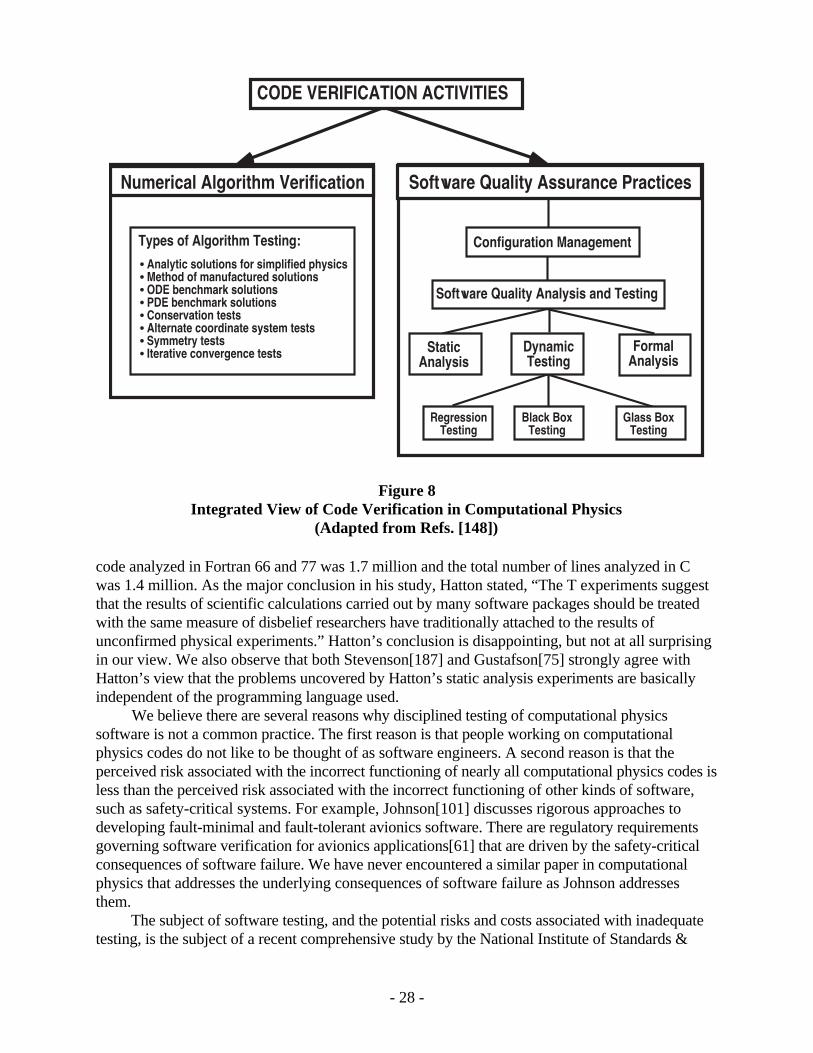
Our view of integrating a set of code verification activities into a verification process forcomputational physics is conceptually summarized in Fig. 8. In this figure we have depicted a top-down process with two main branches: numerical algorithm verification and SQA practices.Numerical algorithm verification, which is the topic discussed in Section 2.3.2, focuses on theaccumulation of evidence to demonstrate that the numerical algorithms in the code are implementedcorrectly and functioning properly. The main technique used in numerical algorithm verification istesting, which is alternately referred to in this paper as numerical algorithm testing or algorithmtesting. The branch of SQA practices, discussed in Section 2.3.3, includes practices andprocedures associated with SQA. SQA emphasizes programming correctness in the sourceprogram, system software, and compiler software. One of the key elements of SQA isconfiguration management of the software: configuration identification, configuration and changecontrol, and configuration status accounting. As shown in Fig. 8, software quality analysis andtesting can be divided into static analysis, dynamic testing, and formal analysis. Dynamic testingfurther divides into such elements of common practice as regression testing, black-box testing, andglass-box testing.
To the disbelief of many, a recent comprehensive analysis of the quality of scientific softwareby Hatton documented a dismal picture.[82] Hatton studied more than 100 scientific codes over aperiod of seven years using both static analysis and dynamic testing. The codes were submittedprimarily by companies, but also by government agencies and universities from around the world.These codes covered 40 application areas, including graphics, nuclear engineering, mechanicalengineering, chemical engineering, civil engineering, communications, databases, medicalsystems, and aerospace. Both safety-critical and non-safety-critical codes were comprehensivelyrepresented. All codes were “mature” in the sense that the codes were regularly used by theirintended users, i.e., the codes had been approved for production use. The total number of lines of
- 27 -
CODE VERIFICATION ACTIVITIES
Types of Algorithm Testing:
• Analytic solutions for simplified physics• Method of manufactured solutions• ODE benchmark solutions• PDE benchmark solutions• Conservation tests• Alternate coordinate system tests• Symmetry tests• Iterative convergence tests
Figure 8Integrated View of Code Verification in Computational Physics
(Adapted from Refs. [148])
code analyzed in Fortran 66 and 77 was 1.7 million and the total number of lines analyzed in Cwas 1.4 million. As the major conclusion in his study, Hatton stated, “The T experiments suggestthat the results of scientific calculations carried out by many software packages should be treatedwith the same measure of disbelief researchers have traditionally attached to the results ofunconfirmed physical experiments.” Hatton’s conclusion is disappointing, but not at all surprisingin our view. We also observe that both Stevenson[187] and Gustafson[75] strongly agree withHatton’s view that the problems uncovered by Hatton’s static analysis experiments are basicallyindependent of the programming language used.
We believe there are several reasons why disciplined testing of computational physicssoftware is not a common practice. The first reason is that people working on computationalphysics codes do not like to be thought of as software engineers. A second reason is that theperceived risk associated with the incorrect functioning of nearly all computational physics codes isless than the perceived risk associated with the incorrect functioning of other kinds of software,such as safety-critical systems. For example, Johnson[101] discusses rigorous approaches todeveloping fault-minimal and fault-tolerant avionics software. There are regulatory requirementsgoverning software verification for avionics applications[61] that are driven by the safety-criticalconsequences of software failure. We have never encountered a similar paper in computationalphysics that addresses the underlying consequences of software failure as Johnson addressesthem.
The subject of software testing, and the potential risks and costs associated with inadequatetesting, is the subject of a recent comprehensive study by the National Institute of Standards &
- 28 -
Technology.[136] This report firmly states: "Estimates of the economic costs of faulty software inthe U. S. range in the tens of billions of dollars per year ..." Precisely where risk-consequentialcomputational physics software lies in this picture remains an important open question.
2.3.2 Numerical Algorithm VerificationNumerical algorithm testing focuses on numerical correctness and performance of the
algorithms. The major components of this activity include the definition of appropriate testproblems for evaluating solution accuracy and the determination of satisfactory performance of thealgorithms on the test problems. Numerical algorithm verification rests upon comparingcomputational solutions to the “correct answer,” which is provided by highly accurate solutions fora set of well-chosen test problems. The correct answer can only be known in a relatively smallnumber of isolated cases. These cases therefore assume a very important role in verification andshould be carefully formalized in test plans for verification assessment of the code.
There are two pressing issues that need to be addressed in the design and execution ofnumerical algorithm testing. The first issue is to recognize that there is a hierarchy of confidence inhighly accurate solutions. The AIAA Guide,[3] for example, suggests the following hierarchicalorganization of confidence for the testing of computational physics codes: (1) exact analyticalsolutions, (2) semianalytic benchmark solutions (reduction to numerical integration of ordinarydifferential equations [ODEs], etc.), and (3) highly accurate benchmark solutions to PDEs.
The second pressing issue in the design and execution of algorithm testing is to chooseapplication-relevant test problems that will be used. There are two possible approaches for makingthis selection. One approach is to pick test problems that people have a great deal of experiencewith. It would be very advantageous if these problems developed into industry standards that couldbe broadly used in verification activities for specific engineering or physics disciplines.Unfortunately, no industry-standard test problems currently exist. A second approach is toconstruct specialized test problems that address specific needs that arise in the structure of the testplan. These test problems are specifically constructed to exercise the portions of the software thatone requires.
Both existing test problems and specially constructed test problems can be either analyticalsolutions or benchmark solutions. Analytical solutions are closed-form solutions to special cases ofthe PDEs that are represented in the conceptual model. These closed-form solutions are commonlyrepresented by infinite series, complex integrals, and asymptotic expansions. Numerical methodsare usually used to compute the infinite series, complex integrals, and asymptotic expansions inorder to obtain the solutions of interest. However, the accuracy of these solutions can be quantifiedmuch more rigorously than can the accuracy of the numerical solutions of the conceptual model.When computational solutions are compared with highly accurate solutions, either the comparisonsshould be examined along boundaries of interest or the error norms should be computed over theentire solution domain. The accuracy of each of the dependent variables or functionals of interestshould be determined as part of the comparisons. Note that the most significant practicalshortcoming of analytical solutions is that they exist only for very simplified physics andgeometries.
A technique for developing a special type of analytical solution to be used for testingnumerical algorithms is the “Method of Manufactured Solutions” (MMS).[112,165,174,177,185]The MMS is a method of custom-designing verification test problems of wide applicability, wherea specific form of the solution function is assumed to satisfy the PDE of interest. This function isinserted into the PDE, and all the derivatives are analytically derived. Typically these derivatives
Using the MMS in code verification requires that the computed source term and boundaryconditions are programmed into the code and that a numerical solution is computed. This techniqueverifies a large number of numerical aspects in the code, such as, the numerical method,differencing technique, spatial-transformation technique for grid generation, grid-spacingtechnique, and correctness of algorithm coding. Shih and his colleagues[178] have applied theMMS to the incompressible Navier-Stokes equations for laminar two-dimensional flow and haveobtained an impressive exact solution to a variant of the classical lid-driven cavity problem for anarbitrary Reynolds number. It is highly recommended that incompressible Navier-Stokes codes beverified with this exact solution.
Knupp and Salari [112] have systematically applied the MMS to Burger’s equation, and thecompressible and incompressible Navier-Stokes equations for laminar flow. These researchershave also presented an interesting study of the “bug-finding” capability of the method to betterunderstand what errors the MMS is capable of resolving. In the study, the performance of theMMS on a set of 21 different coding mistakes was examined. The MMS correctly diagnosed everyerror in the set that prevented the governing equations from being solved correctly. Knupp andSalari (see also Ref. [165]) noted, however, that the MMS is incapable of detecting errors such asalgorithm-efficiency mistakes, which occur in situations where the equations are still solvedcorrectly by the algorithms but the coding is less efficient than is optimal. These results suggest thedesirability of coupling studies like Hatton’s T experiments with a dynamic testing diagnosis likethe MMS to better correlate potential structural flaws with actual incorrect numerical performance.Such a study has yet to be performed.
In numerical algorithm testing the key feature to determine is the observed, or demonstrated,order of accuracy from particular numerical solutions. This should then be compared with theformal order of accuracy of the numerical method. Researchers have found a number of reasonswhy the observed order of accuracy can be less than the formal accuracy. Some of the reasons are:(1) a programming error exists in the numerical algorithm, (2) insufficient grid resolution so thatthe grid is not in the asymptotic convergence region of the Taylor series expansion for theparticular solution variable of interest, (3) the formal accuracy for interior grid points is differentthan the formal accuracy for boundary conditions with derivatives resulting in a mixed order ofaccuracy, (4) singularities, discontinuities, and contact surfaces interior to the domain of the PDE,(5) grid clustering, (6) singularities and discontinuities in the boundary conditions, (7) inadequateconvergence of an iterative procedure in the numerical algorithm, and (8) over-specified boundaryconditions. It is beyond the scope of this paper to discuss these in detail, however some of therepresentative references in these topics are [8,16,18,25,46,64,105,112,165,171,172,184,191]. Itis our view that most of these reasons for degradation in formal order of accuracy are poorlyunderstood and significant research is needed in this area.
Returning to the topic of types of highly accurate solutions, benchmark ODE solutions are
- 30 -
very accurate numerical solutions to special cases of the general PDEs. These solutions commonlyresult from simplifying assumptions, such as simplified geometries that allow solutions in theformation of similarity variables. Benchmark PDE solutions are also very accurate numericalsolutions to special cases of the PDEs or the boundary conditions. The accuracy of the benchmarksolutions, whether ODE or PDE solutions, clearly becomes more of an issue as one moves awayfrom analytical solutions. In the literature, for example, one can find descriptions of computationalsimulations that are considered to be of high accuracy by the author but are later found to belacking. It is strongly recommended that no published solution be considered a numericalbenchmark solution until: (1) the code used in producing the solution has be thoroughly verifiedand documented, (2) very comprehensive numerical error estimation is reported with the solution,and (3) the solution has been accurately calculated by independent investigators, preferably thosewho use different numerical approaches and computer codes.
Consistency tests can also be usefully employed as numerical algorithm tests. Global as wellas regional tests can be made for the conservation of mass, momentum, and energy.[83] A numberof tests can also be made that are related to the effect of numerical boundary conditions on thesolution. One group of tests is used to determine if the same numerical solution is obtained indifferent coordinate systems.[181] Another group of tests is used to evaluate whether certainsymmetry features are preserved in the solution. For example, if a plane of symmetry exists in theconceptual model, then the normal gradient of appropriate variables can be set to zero and asolution can be obtained. The same solution should also be obtained if this plane-of-symmetrycondition is not imposed and the entire domain is solved. For unbounded domains, the boundariesof the computational domain are conceptually considered to be at infinity, i.e., the boundaries areinfinitely far from the spatial region of interest. Typically, a user-defined parameter specifies how"far out" these boundaries are. If the boundaries are too close, the asymptotic conditions appliedthere may not be accurate. The usual method of determining the size of the computational domain isto systematically increase the domain until the solution is no longer dependent on the size of thedomain that is compatible with the objectives of the computation. Consistency tests should beconsidered as complementary to the other types of algorithm tests described in this section.
We believe that the primary responsibility for numerical algorithm verification should beplaced upon the code development team. Computational analysts who are not directly a part of thisteam may conduct the algorithm testing, but we believe the code development team needs to havein-depth knowledge of the algorithms used and their expected performance. This informationshould be documented either as part of the code development process or during testing. Thedocumentation on algorithm testing may be combined with that for SQA testing, as discussed inSection 2.3.3. It is important that analysts and code customers have access to this information.
2.3.3 Software Quality AssuranceSoftware quality analysis and testing, as highlighted in Fig. 8 presented previously, rests in
three techniques: static analysis, dynamic testing, and formal analysis.[195] Static analysistechniques analyze the form, structure, and consistency of the code without executing the code.Examples of static analysis techniques are software reviews and inspections, complexity analyses,audits, and analyses of data flows. Dynamic testing techniques involve execution of the code. Theresults of executing the code are analyzed to detect coding errors or weaknesses in design that cancause coding errors. Regression testing, which re-evaluates the accuracy of computed results, isone example of a dynamic testing technique. Formal analysis, also referred to as formal methods,is directed toward rigorously demonstrating that the code exactly represents the underlyingconceptual model. Further remarks on static, dynamic, and formal analysis are included below.
- 31 -
Two particularly useful books for readers who wish to acquaint themselves with the vast subject ofSQA testing are by Beizer[15] and by Kaner, et al.[104] The differing viewpoints in these booksadd interesting nuances to a subject as seemingly dry (to practitioners of computational physics) asSQA testing. Beizer’s book is somewhat more formal in its approach, while Kaner and hiscolleagues are less structured in their approaches and recommendations.
It is probably safe to claim that static analysis has traditionally been dominated by techniquesto detect compilation errors on the specific code of interest. One does not tend to see publishedstudies of, for example, applying architectural analysis, such as the complexity metrics used inHatton’s analysis,[82] to computational physics codes. We strongly advocate the expansion ofstatic analysis as part of verification assessment for computational physics codes. The complexityof modern programming languages (C++ especially) and the use of massively parallel computingplatforms for computational physics increase the need for, and the impact of, static analysis.
When considering software testing, it is important to understand the distinction betweenglass-box testing and black-box testing. Glass-box testing (also called structural testing) refers totesting when all of the source-code of interest is available. Black-box testing (also called functionaltesting) refers to testing when only the code inputs and code outputs are observable. Glass-boxtesting is practiced primarily by code developers because it assumes sufficient knowledge of thedesign and architecture of the code to design, populate, and assess test plans based on thisknowledge. Glass-box testing is heavily weighted to what we have called SQA testing, althoughthat is not mandatory. When we discuss static analysis, test problems generated by coverageanalysis, and regression testing, we will be discussing examples of glass-box testing. We note thatthe MMS, discussed in Section 2.3.2, is actually code invasive and thus related to glass-boxtesting. The MMS cannot be applied exclusively in black-box mode because of the need forspecific coding intervention for each test that it creates, at least in the examples of which we areaware. Once that coding is accomplished, however, the gathering of results proceeds in a fullyblack-box manner. There does not appear to be any analog of the MMS testing methodology in thework of Beizer[15] and Kaner, et al.,[104] which is rather surprising.
Black-box testing is primarily the paradigm for the algorithm testing discussed above. Black-box testing can be performed by anyone involved with a given computational physics code, but ittends to be associated with independent testing entities. Certainly in the computational physicsworld, much black-box testing is performed by users of the code. (If a developer of the code isalso a user, for purposes of this discussion we emphasize their role as a user.) Black-box testingrequires no detailed knowledge of the code software, although such knowledge can certainly help.Even when those who designed the algorithms and implemented the code execute a test problem toinvestigate the empirical performance of the code, they are performing black-box testing. When acomputational physics algorithm is described in a publication, for example, and compared withsome highly accurate solution, a black-box test has been performed. The goal of the authors in thatcase is to assess the functionality and accuracy of the output results, not to test specific softwareelements. When users test codes by running their favorite test problems prior to application, theyare performing black-box testing. Users are an enormous resource for black-box testing. In ourdiscussion of dynamic testing, aspects of regression testing, and statistical testing, we areaddressing issues that are particularly relevant to black-box testing. The goal of a coordinated,optimal test strategy for a computational physics code is to blend black-box testing and glass-boxtesting.
Coverage analysis and code sensitivity analysis are methods that can be used to assess thecomplexity of the computational physics code in order to design collections of test problems.Coverage analysis enables one to determine what components of the code enter into various
- 32 -
options exercised in the code. The relative importance of the selected component contributions tothat calculation is then determined via a sensitivity analysis. Ideally, one would start coverageanalysis with a tool of sufficient capability to assess code lines and units exercised by the code inperforming the desired calculation. For example, PureCoverage™[160] is a commercial tool thatdetects lines of code executed during the operation of C++ software and reports this information ina useful form. A major challenge of coverage analysis for algorithm testing is to understandexecution paths as well as lines touched in the code in order to execute the intended applicationcalculation. One then designs tests that specifically target these modules and paths. This is clearly aglass-box-testing strategy and is discussed extensively in both Beizer[15] and Kaner, et al.[104]While a discussion of sensitivity analysis is beyond the scope of this paper, the topic is brought upin the context of software quality testing in Ref. [138].
A natural partner of coverage analysis for software quality testing is regression testing. Awidely used commercial testing technique, regression testing is defined by Beizer[15] as “anyrepetition of tests (usually after software or data change) intended to show that the software’sbehavior is unchanged except insofar as required by the change to the software or data.” What thismeans in practice for computational physics is that a compendium of tests is assembled, a baselinefor code performance against these tests is established, and the tests are run periodically. When thecurrent performance is determined to have deviated from the baseline, either the decision is madethat a bug has been introduced or the regression test suite is baselined again. There are tworequirements that make this approach feasible. First and foremost, the test suite must runsufficiently fast so that the testing can be performed frequently. Second, the regression testingshould be performed for every software modification. For multiple developers of a computationalphysics code, for example, this means that no modified software is accepted before regressiontesting is performed. This, of course, can impede the software development process if notmanaged properly.
Regression tests that are glass-box tests are often correlated with coverage analysis anddesigned to provide testing of as many lines of code as possible. Systematic, cyclic-regressiontesting, once a suitable set of test problems has been defined, is known to be important in codedevelopment and maintenance. Unfortunately, this requires a trade-off between available resourcesthat influences the fidelity of the testing. For example, a high-fidelity test suite that takes longerthan 5 to 10 hours to execute is probably not practical for execution every day. Thus, such a suitecannot be used to demonstrate the stability of daily code builds.
The main use of regression testing is to minimize the effort devoted to fixing incorrect newsoftware that is introduced into existing code in a software development project. There is a balancethat must be determined between the effort devoted to regression testing and the effort devoted tofinding and fixing incorrect modifications of the existing code at a later date. At the same time,regression testing aims to cover as much of the code as possible. In the computational physicsprojects that we are familiar with, the anticipated coverage target for regression testing is typicallyon the order of 80% of the lines of code. Accepting 80% line coverage is commonly based on thedevelopers willingness to define specific code elements as not requiring coverage. Moreimportantly, these coverage thresholds are established in the attempt to prevent the effort devoted toregression testing from becoming larger than the effort required to fix introduced errors.
A great deal of effort has recently been devoted to the development and application of formalmethods.[20,154,173] However, the actual goal of these methods—rigorous “proof” that a systemof software is correctly implemented—remains controversial in our opinion. The application offormal methods is also complicated by disputes over cost, appropriateness, utility, and impact.[19]
- 33 -
Formal methods have certainly not been applied to software systems like those of interest incomputational physics, namely, those systems in which floating-point arithmetic is dominant andan effectively infinite variability in software applications is the norm. The utility of these methodsto computational physics codes, even if resource constraints were not issues, has not beenestablished. This fact has led to interest in the application of formal methods to more restrictedproblems that still may be of significant interest in computational physics software. For example,there is current interest in applying formal methods to aid in verification of the mathematicalformalism of the conceptual model that underlies a computational physics code rather than in thefull details of the software implementation.[33,116]
We conclude this section on SQA by providing a few brief remarks and references for someof the key literature that is relevant to the overall problem of verification assessment. A number ofmodern texts are available that describe current practice in the SQA field.[9,15,40,42,55,62,102,124,157,169] Much of the research and development in SQA procedures has been fueled bycomputer-controlled systems that require extremely reliable and secure software, as in Johnson’savionic-systems application referenced previously. Such systems are commonly referred to as“high-integrity systems.” Examples of other high-integrity systems are control systems for nuclearpower reactors and software for nuclear-weapon security and safety. The scientific softwarecommunity has much to learn from SQA procedures that have been developed for these systems ashigh-consequence scientific computing becomes more prevalent. This includes an improvedunderstanding of the responsibilities associated with producing high-integrity computationalphysics codes.
2.3.4 Numerical Error EstimationThe two basic approaches for estimating the error in a numerical solution to a PDE are a
priori and a posteriori approaches. An a priori approach uses only information about thenumerical algorithm that approximates the partial differential operators and the given initial andboundary conditions. A priori error estimation is a significant element of classical numericalanalysis for PDEs, especially those underlying the finite element and finite volume methods.[64,93,94,117,133,149,165] An a posteriori approach uses all of the a priori information, pluscomputational results from a previous numerical solution using the same numerical algorithm onthe same PDE and initial and boundary data. In this paper we also refer to a posteriori errorestimates as “empirical” data or, as Roache[165] calls it, “observed” data. Empirical data could be,for example, a solution on a single coarse grid or a sequence of solutions on consecutively finergrids. We believe the only quantitative assessment of numerical error that can be achieved inpractical cases of nonlinear PDEs is through a posteriori error estimates. As a result, only aposteriori will be discussed here.
A posteriori error estimation has primarily been approached through the use of eitherRichardson extrapolation[165] or estimation techniques based on finite element approximations.[4,12] Richardson’s method can be applied to both finite difference methods and finite elementmethods. As pointed out by Roache,[165] Richardson’s method produces different estimates oferror and uses different norms than the traditional a posteriori error methods used in finiteelements.[94,162] A Grid Convergence Index (GCI) based on Richardson’s extrapolation hasbeen developed to assist in the estimation of grid convergence error.[163-165] The GCI convertserror estimates that are obtained from any grid-refinement ratio into an equivalent grid-doublingestimate. Recent studies have shown that the GCI method is fairly reliable, even for solutions thatare not in the asymptotic-convergence region.[23,27,59,170]
Richardson’s extrapolation can be applied to compute error estimates of dependent variables
- 34 -
at all grid points, as well as error estimates for solution functionals. Solution functionals areintegrated and differentiated quantities such as body lift and surface heat flux, respectively. Vendittiand Darmofal[193] discuss the coupling of error estimation and adaptive grid generation to reducenumerical errors in such computed functionals. Their particular example is the quasi-one-dimensional flow in a variable-area duct. It is important to emphasize that different dependentvariables and functionals converge at different rates as a function of grid size. For example, thegrid and time step that are required to show second-order convergence in heat flux on a bodysurface are extremely finer than for total lift on a body. This fact was also pointed out by earlierresearchers,[100,165] as well as in the AIAA Guide.[3]
A posteriori error estimates are also important for finite element adaptivity, where both thespatial grid density (h-adaptivity) and the order of the finite element scheme (p-adaptivity) can beadapted. The important role of a posteriori estimates in adaptivity for finite elements is discussedin many papers, as well as in the recent books by Ainsworth and Oden[4] and Babuska andStrouboulis.[12] For numerical error estimation, however, finite element adaptivity is not theissue. Although traditional a posteriori methods used in finite elements are very useful andcomputationally efficient, these methods do not demonstrate asymptotic convergence or directlyaddress useful engineering error measures. Recent work in a posteriori error estimation addresseserror in local quantities of engineering interest, as well as error estimation for certain types ofnonlinearities in elliptic problems.[4,12] Regardless of the a posteriori error estimation approachchosen, the estimation should always be made for the system response outputs that are relevant tothe application of interest.
The assumption of smoothness in solutions, i.e., no singularities and discontinuities, isquite demanding in estimating local errors in the solution domain. Singularities and discontinuitiescommonly occur in fluid dynamics, solid mechanics, and structural dynamics. The “pollution” ofparticular regions of a calculation by the presence of singularities such as shock waves, geometricalsingularities, or crack propagation is a subject of grave concern in error estimation. Often, the onlyclear sense of this pollution available to us is through careful empirical assessment. Since thetechnical aspects of this issue are beyond the scope of this paper, the reader should consult a seriesof papers by Babuska and his colleagues[10,11,13] as well as the paper by Oden[150] for adiscussion of this problem from a finite-element point of view. Roache[165] has a wide-rangingdiscussion of this topic, and the recent work of Zhang and his colleagues[203] discusses how thepresence of a shock wave structure affected a posteriori error estimates for the Euler equations. Arecent paper of Botella and Peyret[18] discusses similar problems associated with computingsingular solutions of the Navier-Stokes equations.
An additional numerical error estimation complexity should be mentioned that can occur incertain types of computational physics simulations. This complexity can be conceptually describedas a coupling between numerical error and the appearance of new spatial and temporal scales incertain types of physical models. In fluid dynamics, for example, when grids are sufficientlyrefined, completely new processes or characteristics on the smaller spatial scales can develop. It isnot uncommon that a steady flow field can become unsteady as the grid is refined and very small-scale phenomena can develop that did not exist on the coarser grids. This occurs in the case of thetrailing edge region of a compressor or turbine blade, where vortex shedding is known to exist andwill appear in the simulation if the grid around this region is sufficiently refined. Refining gridsdoes not ensure that the physics modeled will remain unchanged as the grid is resolved. Thisobservation directly influences the accuracy and reliability of any type of a posteriori errorestimation method, especially extrapolation methods.
Extracting an estimate of numerical accuracy on underresolved grids is a topic of current
- 35 -
research. We previously mentioned one aspect of the problem, generically referred to as pollutionerror—the propagation of discretization error from less accurately resolved regions of a calculationinto more accurately resolved regions. Another issue is simply to understand what information canrationally be synthesized from calculations with more- or less-known resolution accuracy. Thoughthis topic is beyond the scope of this paper, Chorin[30-32] and Glimm[70,73] demonstrate thattechniques for understanding the numerical accuracy of underresolved calculations are challengingand specialized. A critical theme in this literature, and one that might be generalized to otherimportant problems, is the role of probability and statistical estimation in performing suchassessments. We conclude by commenting that studying V&V for underresolved calculationsdirectly addresses the challenges posed by Gustafson in his 1998 paper.[75]
2.4 Validation Activities
2.4.1 Fundamentals of ValidationWe have emphasized that validation experiments must be designed purposefully with specific
goals linked to application objectives and to specific elements of the PIRT. The primary goal ofdirected validation experiments is to ensure that experimental data are sufficiently related to theapplication driver to provide stringent confidence assessment when code calculations are comparedwith these data. These data must be precisely located within the structure of the application-specificPIRT and must be unambiguous in defining confidence in the application of the code to thephenomena exemplified in the experiment. Because this task must be accomplished byquantitatively comparing code calculations with experimental data, important requirements areplaced on validation experiments to create the greatest opportunities for performing thesecomparisons. It is critically important to design and execute validation experiments that allowprecise and conclusive comparisons of calculations with experimental data for the purpose ofassessing model fidelity and credibility. In Section 2.4.5 we further discuss model-experimentcomparisons. It will hopefully be made clear that the design and execution of experiments mustallow us to quantify meaningful and useful metrics.
Particular validation experiments may achieve these goals to a greater or lesser degree, butany such attempt rests on a foundation of rational design concepts that are based on the needs ofthe application of the code. The more purposefully we design an experimental validation activity,the greater the probability that we can optimize the results of that activity in the face of thesecomplex constraints. It is important from an engineering perspective that validation experimentsbalance resource constraints, including time, level of effort, available expertise, and desiredfidelity. The approach for achieving this balance should be defined in the experimental plan. Howto achieve this balance will depend strongly on which tier of physics complexity the experiment isconducted. As briefly mentioned in Section 1.2, validation experiments can be conducted at theunit-problem, benchmark, subsystem, or system tier. The resources needed vary greatly from onetier to the next. Section 2.4.2 discusses some of these topics in more detail.
The experimental, computational, and comparison activities should expedite the quantitativeassessment of computational models for system applications that are within the application domain.It is important to attempt to quantify the boundary separating the region of acceptability of themodel from the region where the model is not acceptable for the application. Designingexperiments that test a model in regions where the model is believed to be insufficiently accuratefor the intended application helps locate this boundary and provides a means for quantitativelyassessing the degree of the expected inaccuracy. Because such experiments are performedpurposefully rather than accidentally, these experiments also further test our grasp of the
- 36 -
conceptual models underlying the code that are probed by the validation experiments. Obviously,this goal only makes sense when experiments that probe model inaccuracy lie close enough to theboundary of applicability to be relevant. It is desirable to have experimental validation tasks thathave the explicit goal of defining those application domains where use of the model is questionablyadequate to better quantify the boundary of applicability of the model. To perform these validationtasks in a conscious and scientifically directed manner is not necessarily any easier than to achievedesirable levels of confidence in other application domains.
Figure 9 illustrates a typical relationship between the application domain and the validationdomain. The relationship between the application domain and the validation domain shown in Fig.9 is actually part of the class of relationships shown in Fig. 5b: the application domain is not asubset of the validation domain. Two kinds of points are shown in Fig. 9. An “C” denotes alocation in the parameter-complexity space where a computational result in the application domainhas previously been performed; a “V” denotes a location in the space where a validationcomparison between computation and experiment has been performed. The boundary of thevalidation domain represents the apparent limit where the physical models in the code would nolonger be reliable. The boundary of the validation domain could be estimated, for example, byusing alternate plausible computational models or by using expert opinion. We draw the reader’sattention to two pairs of intended applications, each pair denoted “CI” and “CO”. The applications“CI” each lie inside of the validation domain, while the applications “CO” each lie outside of theapparent validation domain. Our point is that it is essentially as important from an engineeringproject perspective to know that the model is questionable for the applications “CO” as it is to knowthat the model is acceptable for the applications “CI”.[129,201] An extensive validation effort couldidentify the validation boundary accurately, but such an effort is commonly not possible, forexample, because of programmatic schedules, budgets, safety and environmental concerns, orinternational treaties.
ApplicationDomain
ValidationDomain
V
VV
V
V
V
VV
CO
C
CI
system or environmental parameter
ph
ysic
al a
nd
geo
met
rica
l co
mp
lexi
ty
CO
CI
C computational result has been obtainedV validation comparison has been made
C
C
C
C
C C
Figure 9Typical Relationship Between the Application Domain and the Validation Domain
(adapted from Ref. [190])
- 37 -
There should be a well-reasoned basis for choosing between two potential validationexperiments. The basis should depend on the potential benefits of defining the acceptable domainboundary and on the use of available time and resources. The prioritizations embodied in the PIRTshould be helpful in choosing between the two potential experiments. In partnership with thePIRT, two approaches are recommended: competing alternate plausible models and statisticalexperimental designs. Competing alternate plausible models can be of two different types: alternatemodels that are generally at the same level of modeling fidelity, and hierarchical models. Usinghierarchical models, one formulates conceptual models that are clearly at different levels of fidelityor physical detail. Results from the models at different levels of complexity are compared toattempt to assess where the lower fidelity model could begin to fail. Statistical experimental design(for example, see Cox[38] and Dean and Voss[41]) is an attractive basis for attacking the resourceoptimization problem for experiments with a focus on uncertainty quantification. Gunter[74] hasargued in favor of using statistical experimental design in planning physical-science experiments.The specifics of how the statistical design of experiments may be applied in particular validationactivities are dependent upon the subject-matter focus of these experiments.
2.4.2 Construction of Validation Experiment HierarchyAny appropriate methodology for the purposeful definition, design, and analysis of
experiments for validation of a code must consider the intended application. As discussed inSection 2.2, the PIRT is the key methodology for identifying the predictive-capability needs andsetting the validation priorities. To implement the needs and priorities identified in the PIRT, therecommended methodology is the use of a validation hierarchy, as discussed in Section 1.2. Thehierarchical view of validation is distinctly an engineering perspective, as opposed to a scientific ormodel-building perspective. The purpose of the validation hierarchy is to help identify a range ofexperiments, possible separation of coupled physics, and levels of complexity—all of which arerelated to an engineering system—so that computer codes from different disciplines can beevaluated. Stated differently, the validation hierarchy must be application driven to be ofengineering value, not code capability driven.
As one constructs each lower tier of the hierarchy, the emphasis moves from multiplecoupled-physics codes to single codes (or single-physics options in multi-physics codes)simulating a particular type of physics. In parallel with the simplification process, the focus on theactual operating conditions of the complete system should not be lost. Constructing thesehierarchical tiers and identifying the types of experiments that should be conducted at each tier areformidable challenges. There are many ways of constructing the tiers; no single construction is bestfor all cases. We would draw the analogy of constructing validation hierarchies to the constructionof control volumes in fluid-dynamic analyses. Many varieties of control volumes can be drawn;some lead nowhere, and some are very useful for the task at hand. The construction shouldemphasize the modeling and simulation capability that is desired to be validated, whether thatcapability is computational physics or other computational disciplines. Analogous tier structurescan be developed for structural dynamics and electrodynamics, for example, when the engineeringsystem of interest involves these disciplines.
A good hierarchical tier construction is one that accomplishes two tasks. First, theconstruction carefully disassembles the complete system into tiers in which each lower-level tierhas one less level of physical complexity. For complex engineered systems, this may require morethan the three building-block tiers shown in Fig. 2, presented previously. The types of physical
- 38 -
complexity that could be uncoupled from one tier to the next are spatial dimensionality, temporalnature, geometric complexity, and physical-process coupling. The most important type of physicalcomplexity is physical-process coupling, which commonly contains the highest nonlinearity of thevarious contributors. The nonlinear coupling is, of course, eliminated by conducting experimentswith uncoupled and separate physical effects, e.g., separating turbulence and combustion. It isimportant to recognize the potential nonlinear nature of all of the contributors in the construction ofthe tiers because the philosophy of the tier construction rests heavily on linear-system thinking.That is, the belief that confidence in the computational capability for the complete system can bebuilt from an assessment of the computational capability of each of its parts. The complete systemsof interest clearly do not have to be linear, but the philosophy of the hierarchical validationapproach loses some of its utility and strength for strong nonlinear coupling from one tier to thenext.
The second task accomplished by a good hierarchical tier construction is the selection ofindividual experiments in a tier that are practicably attainable and able to produce validation-qualitydata. In other words, the individual experiments should be physically achievable given theexperimental test facilities, budget, and schedule, and they should be capable of producingquantitative experimental measurements of multiple system-response measures that can test themodel in question. For complex systems, the ability to conduct a true validation experiment at thecomplete system tier is extremely difficult, if not impossible. At the subsystem tier, it is usuallyfeasible to conduct validation experiments, but it is still quite difficult and expensive. One usuallychooses a single hardware subsystem or group of subsystems that are closely related in terms ofphysical processes or functionality. For complex subsystems, one might want to add a new tiercalled “components” below the subsystem tier. As with the subsystem tier, the components tierwould consist of actual operational hardware components. When one defines the individualexperiments at the benchmark-tier level, special hardware should be fabricated. By “specialhardware” we mean that the hardware need not be constructed to perform its system tier orsubsystem tier functions.
The benchmark tier is probably the most difficult to construct because it represents thetransition from a hardware focus in the two top tiers to a physics-based focus in the bottom tiers ofthe hierarchy. At the bottom tier, unit problems, one should identify simple geometry experimentsthat have a single element of physical-process complexity. As with the subsystem tier, anadditional tier may need to be added to attain only one element of physics at the bottom tier. Also,the experiment must be highly quantitatively characterized so that it can provide the necessary datato the computational code, and the experiment must be conducted so that experimental uncertaintycan be estimated precisely. High-quality validation experiments are practicably attainable at thebenchmark and unit-problem tiers, but usually not at the system or subsystem tiers for complexsystems.
Recently, an example of a hierarchical tier structure for a complex, multidisciplinary systemwas presented in Ref. [147]. The example features an air-launched, air-breathing, hypersoniccruise missile. The missile is referred to as the complete system, and the following are referred toas systems: propulsion, airframe, guidance, navigation, and control (GNC), and warhead. Theexample assumes that the missile has an autonomous GNC system, an on-board optical targetseeker, and a warhead. Figure 10 shows the system-level hierarchical validation structure for thehypersonic cruise missile. The structure shown is not unique, nor is it necessarily optimum forevery computational-simulation perspective of the missile system. In addition, the structure shownin Fig. 10 focuses on the airframe system and the aero/thermal protection subsystem for thepurpose of analyzing the aero/thermal performance of the missile.
- 39 -
Lowtemperaturesublimation
Boundarylayer
transitionover simple
bodies
Shockwave/turbulentboundary
layerinteraction
Turbulenthypersonicflow with
wallblowing
Turbulenthypersonicflow over
simplebodies
Laminarhypersonicflow with
wallblowing
Laminarhypersonicflow over
simplebodies
Non-isotropic
heatconduction
LaminarHypersonicFlow WithAblation
TurbulentHypersonicFlow WithAblation
BoundaryLayer
TransitionWith
Ablation
Ablation OfThermal
ProtectiveCoating
HeatTransferTo Metal
Substructure
StructuralSubsystem
ElectrodynamicsSubsystem
Navigation andGuidance,
Control
WarheadSystem
PropulsionSystem
Couplesto GNC
Couplesto GNC
BENC
HMAR
K
UNIT
PRO
BLEM
TIER
SUBS
YSTE
MSY
STEM
Couples to structural
subsystem and connects
to benchmark tier
Protection SubsystemAero/Thermal
TIER
TIER
TIER
AirframeSystem
SYST
EMTI
ER
COM
PLET
E
Figure 10Validation Hierarchy for a Hypersonic Cruise Missile[147]
To better demonstrate how the validation hierarchy of the aero/thermal protection subsystemis related to the validation hierarchy of the propulsion, airframe, GNC, and warhead systems, theexample was discussed further in Ref. [147]. Figure 11 shows how the validation hierarchy ofeach of these four systems could be viewed as the primary facets of a four-sided pyramid. Theairframe facet was divided into three additional facets, each representing the three subsystems:aero/thermal protection, structural, and electrodynamics. The propulsion system was divided intofour additional facets to represent its subsystems: compressor, combustor, turbine, and thermalsignature. Similarly, the GNC and the warhead systems could be divided into subsystemsappropriate to each. On the surface of this multifaceted pyramid, one can more clearly and easilyindicate the coupling from one facet to another. For example, we discussed the coupling of laminarand hypersonic flow with ablation to the optical seeker of the GNC system. This coupling wouldbe shown by an arrow connecting these hypersonic flow elements to appropriate elements on theGNC facet of the pyramid. (Suggested references stressing a systems engineering perspective areRefs. [17,76,119,144,202].)
- 40 -
PROPULSIONSYSTEM AIRFRAME
SYSTEM
Aero/thermal
Protection Subsystem
Structual
SubsystemElectrodynamics
SubsystemCompr
esso
r
Subs
ystem
Com
bust
orSu
bsys
tem
Turb
ine
Subs
yste
m
Ther
mal
Sig
natu
reSu
bsys
tem
WARHEADSYSTEM
GUIDANCE, NAVIGATION& CONTROL SYSTEM HYPERSONIC
CRUISE MISSILE
Figure 11Validation Pyramid for a Hypersonic Cruise Missile[147]
The validation pyramid stresses the systems-engineering viewpoint in modeling andsimulation-based design, as opposed to the viewpoint of a specific discipline. Each facet of thepyramid can then be devoted to identifying validation experiments for each computational modelresponsible for part of the design of the complete system. As one traverses around the top of thepyramid, the number of facets is equal to the number of systems that are identified. As onetraverses around the bottom of the pyramid, the number of facets is equal to the total number ofmajor computer codes used in the analysis of the engineering system, i.e., the number of codesthat require validation activities for the intended application. For the example of the hypersoniccruise missile, if the code that simulates surface ablation is a separate code from the aerodynamicscode, then an additional facet on the pyramid is added on the aero/thermal subsystem facet. Westrongly believe this type of system-level thinking is necessary to increase confidence in complexsystems that are designed, manufactured, and deployed with reduced levels of testing.
2.4.3 Characteristics of Validation ExperimentsMany researchers, analysts, and managers ask: What is a validation experiment? or How is a
validation experiment different from other experiments? These are appropriate questions. Wesuggest that traditional experiments could generally be grouped into three categories. The firstcategory comprises experiments that are conducted primarily to improve the fundamentalunderstanding of some physical process. Sometimes these are referred to as physical-discoveryexperiments. The second category of traditional experiments consists of those conducted primarilyfor constructing or improving mathematical models of fairly well-understood physical processes.The third category of traditional experiments includes those that determine or improve thereliability, performance, or safety of components, subsystems, or complete systems. Theseexperiments are commonly called “tests” of engineered components or systems.
We argue that validation experiments constitute a new type of experiment. A validationexperiment is conducted for the primary purpose of determining the validity, or predictive
- 41 -
accuracy, of a computational modeling and simulation capability. In other words, a validationexperiment is designed, executed, and analyzed for the purpose of quantitatively determining theability of a mathematical model and its embodiment in a computer code to simulate a well-characterized physical process. Thus, in a validation experiment “the code is the customer” or, ifyou like, “the computational analyst is the customer.” Only during the last 10 to 20 years hascomputational simulation matured to the point where it could even be considered as a customer. Asmodern technology increasingly moves toward engineering systems that are designed, andpossibly even fielded, based on modeling and simulation, then modeling and simulation itself willincreasingly become the customer of experiments.
In our view, there are three aspects that should be used to optimize the effectiveness andvalue of validation experiments. The first aspect is to define the expected results of theexperimental validation activity using the code itself. The second aspect is to design specificvalidation experiments by using the code in a predictive sense. The third aspect is to develop awell-thought-out plan for analyzing the computational and experimental results. These aspectsemphasize tight coupling of the subject code to the experimental activity and ensure we are in thebest position to learn from the comparison of computational and experimental results, regardless ofwhether these comparisons are good or bad, as explained below.
Consider the second aspect above related to the design of a validation experiment. Suppose,through a series of exploratory calculations for a particular application of the code, that anunexpectedly high sensitivity to certain physical parameters appears. Specific PIRT elements forthe application may have postulated little sensitivity to the parameters, or the PIRT may have statedthat the sensitivity was unknown. If this unexpected sensitivity has an important impact on theapplication of interest, a validation experiment assessing the correctness of this sensitivity shouldbe pursued. The code that is the object of the validation exercise should participate in defining theprinciples and goals of a planned validation experiment. An alternative phrase to keep in mindwhen the word “define” appears is “define the purpose of the experiment.” The role of the code inthe definition of validation experiments may be purely exploratory until some progress has beenmade on validation activities.
One way of designing a validation experiment is to use the code calculations as specificguidance on where to locate the instrumentation and what kind of data to acquire for assessing theanticipated sensitivity. In the proposed validation experiments, “design” means specifying to thegreatest degree possible the initial and boundary conditions, material properties, diagnosticlocations and characteristics (strain gauge? temperature gauge?), and data fidelity. The probabilitythat these conditions, “defined” through code calculations, will be met precisely in any complexvalidation experiment is probably zero, but the probability that they will be met in simplerexperiments is relatively high. In most cases, the success of a validation experiment will often bedetermined by the degree to which the experiment matches these specifications. Deviations can beacceptable; but if the intent of the experiment was to measure x at location y for material z andgeometry g and in all cases the experiment is significantly different from most or all of thesefactors, it is unlikely that the experiment would be a successful validation experiment.
Engaging a code in the definition and design of validation experiments can easily bedistinguished from more common experimental practice. In the conventional case of nonvalidationexperiments, the experimenters state the following to the computational analyst in the typicalapproach: “We are performing the following experiment. Tell us what the expected response ofgauge a will be, given this experimental design and location for the gauge.” For a validationexperiment, on the other hand, the computational analyst makes the following statement to the
- 42 -
experimenter: “Please perform the following experiment. We recommend locating gauge a atlocation x based on our computational predictions. It will be very useful to see whether ourpredictions agree with your experiment. If your experiment has deviated from our requesteddesign, we still anticipate achieving useful validation consequences through furtherpostexperimental analysis, as long as the design deviation is not great.”
A number of researchers, particularly experimentalists, have slowly been developing theconcepts of a validation experiment. During the past several years, a group of researchers at SandiaNational Laboratories has been developing philosophical guidelines and procedures for designingand conducting a validation experiment. Although the following six guidelines and procedureswere developed in a joint computational and experimental program conducted in a wind tunnel,they apply over the entire range of computational physics:[1,2,140-143,194]
Guideline 1: A validation experiment should be jointly designed by experimentalists, modeldevelopers, code developers, and code users working closely together throughout theprogram, from inception to documentation, with complete candor about the strengths andweaknesses of each approach.
Guideline 2: A validation experiment should be designed to capture the essential physics ofinterest, including all relevant physical modeling data and initial and boundary conditionsrequired by the code.
Guideline 3: A validation experiment should strive to emphasize the inherent synergismbetween computational and experimental approaches.
Guideline 4: Although the experimental design should be developed cooperatively,independence must be maintained in obtaining both the computational and experimentalresults.
Guideline 5: A hierarchy of experimental measurements of increasing computationaldifficulty and specificity should be made, for example, from globally integrated quantitiesto local measurements.
Guideline 6: The experimental design should be constructed to analyze and estimate thecomponents of random (precision) and bias (systematic) experimental errors.
The purposeful design of validation experiments is enabled and accomplished through adiverse team of people who participate in the experimental validation activity. Most obviously, oneor more experimentalists are participants in this team. However, code users (analysts, designers)must also participate, given our proposed primary role of the code in the definition, design, andanalysis of validation experiments. Finally, one or more code developers should be on thevalidation experiment team. Their presence provides valuable expert knowledge about theperceived a priori capability of the code in all three aspects of experimental validation: define,design, and analyze. In fact, code developers, including experts on the physical models in thecode, are the most knowledgeable about the boundary of the acceptable application domaindiscussed in Fig. 9.
Validation experiments should not produce data that fundamentally depend on codecalculations for critical data-reduction tasks. Such data do not correctly address our need for
- 43 -
independent comparability of experimental data with calculations and violate our need forrobustness of the experimental data. Experimental data that require code calculations for evaluationcan never be a desirable outcome for a validation experiment, although exactly this problem mayarise in other kinds of experiments. An example of what we mean is the problem of inference ofmaterial temperature from experimentally acquired shock hydrodynamic data (density, pressure,and velocity fields) using code calculations of shock-wave physics rather than some type ofdiagnostic to directly measure the temperature. The only possible validation data that will emergefrom shock hydrodynamics experiments without temperature diagnostics are the shockhydrodynamic data. This problem is relevant, since it arises in investigations of temperaturedependence in high-pressure shock-driven material response. Such experiments often need codecalculations to estimate the associated thermal conditions under shock loading. For purposes ofscientific discovery, this is permissible though speculative. Such experiments, however, cannot beclaimed to provide validation data for the high-pressure thermomechanical response of the materialbecause of the lack of independence of calculations and experiment.
Attempting to sharply define the boundary of applicability of the code for a given applicationdomain through a deliberate choice of experiments close to the boundary, but on the invalid side,has greater leverage when code predictions are used to design such experiments. We stress onceagain that achieving a satisfactory level of performance for the code in comparison with validationexperimental data in a case of true prediction has far greater power to raise our level of confidencein the application of the code. We may not be able to quantitatively measure this fundamentalobservation at this time, but it is obviously true. Predictive accuracy is gold, while posttestconsistency is merely brass at best and possibly fool’s gold at worst.
2.4.4 Uncertainty Quantification in ComputationsAs mentioned in Section 2.4.1, it is common when simulating validation experiments that
one encounters physical parameters, e.g., in the PDEs or in the initial or boundary conditions, thatare not precisely known or measured for an experiment. This situation is much more common atthe system and subsystem tiers than at the benchmark and unit-problem tiers. Examples of suchparameters are thermochemical transport properties, flow rates in complex systems, and inflownonuniformities. Another common situation occurs during a series of experiments, e.g., weather-driven experiments and flight tests, when there are certain parameters that are poorly controlled ornot controllable at all. For any parameter, we make the assumption that a value of that parameter isrequired to perform the computational simulation. The situations just mentioned are allcharacterized by stochastic parametric uncertainty. In the following discussion, we simply refer to“uncertainty,” but we will always be referring to parametric uncertainty. This type of uncertaintyrequires nondeterministic simulations in validation of computational physics.
One standard approach is to estimate, by one means or another, a single value of such aparameter and compute a solution with that selected value. This might be a fully adequate way ofdealing with this uncertainty, especially if experience suggests that the range of potential parametervalues is very small and that the calculation is known not to be extremely sensitive to the parameterin question. The resulting calculation intrinsically is interpreted as “representative,” or “bestestimate” or “conditional” for that parameter.
The shortcomings with the standard approach referred to above begin to be noticeable whenthe range of variation of the parameter is large or when the calculation is known to be sensitive tothe parameter values. If multiple required parameters in a computation of a validation experimentare uncertain, it is entirely possible that the interaction of these parameters in the calculation maymagnify the influence of their uncertainty on the final results of the calculation. In our opinion, this
- 44 -
statement is especially important when performing calculations that are intended for directquantitative comparison with validation experiments. We believe that the uncertainty of theparameters should be incorporated directly into the computational analysis.
The simplest strategy for incorporating uncertainty of this kind directly into the computationis performed in three steps. The first step, called characterizing the source of uncertainty, is basedon the assumption that the uncertainty in the parameters of interest is characterized by probabilitydistributions. Sometimes such distributions can be directly estimated if a large quantity ofexperimental data is available for the parameters. Sometimes such distributions simply must beassumed. At any rate, the first step involves specifying the probability distributions andunderstanding the credibility of these assumptions.
In the second step, ensemble computing, values from the input probability distributionsspecified in the previous step are selected using statistical sampling procedures, such as MonteCarlo or Latin Hypercube sampling methods (see, for example, Refs. [39,67]). These sampledvalues are then used in a set of computations. Because this latter statement is so important, we willrestate it. The assumed prior probability distributions for the uncertain parameters are used togenerate a set of calculations. This set is sometimes called an ensemble of calculations.
The key issue is that a single calculation is no longer sufficient; a set of calculations must beperformed. Obviously, this need is disturbing; where once one might have performed a singlecalculation, now one must perform a potentially large number of calculations. We have not raisednor answered the question of whether sufficient computational resources are available to executemore than the one calculation. However, the constraints enforced by the availability of computingmay be formidable.
After the set of calculations has been generated, the third step, uncertainty quantification ofthe output, is performed. This step involves analysis of the set of calculations, typically usingstatistical inference, to estimate a probability distribution for the output variables of interest thatresults from the given input parameter distributions. In general, we cannot deduce the exact outputdistribution that results from the assumed form of the parameter distributions used to generate thecomputational input associated with those parameters. Instead, the common practice is to usestatistical procedures to determine estimates of important parameters associated with that outputdistribution.
Such statistically determined estimates are useful for comparing computational results withexperimental measurements. For example, the mean of the output calculations provides us with anestimate of the expected value of the output quantity of interest, given the uncertainty structurespecified by the input distributions. This mean-value estimate is of primary importance whencomparing computational results with the mean value of multiple experimental realizations. Anotherstatistic of interest is the estimated variance of the output distribution, which can be interpreted as ameasure of computational output uncertainty, or scatter, given the input uncertainty.
For readers unfamiliar with this methodology, we stress that it is rarely true that the mean ofthe output, given the input uncertainty, can be determined by performing a calculation for a singleset of inputs that is chosen to be the mean of each of the input distributions. Stated in another way,the mean value of the output cannot be computed by performing a simulation using the mean valueof all input parameters, except when the mapping of inputs to outputs is linear in the parameters.Linearity in the parameters essentially never occurs when the mapping of inputs to outputs is givenby a differential equation, even a linear differential equation. Instead, we must perform theensemble of calculations to develop a statistically rational estimator for the mean. The previousstatement is also true for estimating other output statistics. Kleijnen[106] provides a broadsummary of methodologies that go beyond Monte Carlo for assessing output distributions
- 45 -
statistically.In summary, the general methodology we are thus advocating for incorporating parameter
uncertainty into computational physics computations is to execute all three steps in the mannersuggested above. Performing the three-step strategy will clearly be nontrivial for hardcomputational problems simply because of the computational burden imposed. There are alsocertain subtleties that we have not mentioned, such as whether complex structure in the resultingoutput probability distribution can actually be discovered using such a crude approach. Extractingan intricate output-distribution structure will require either a large number of sample input values orconsiderably more sophisticated approaches for performing the methodology. The only modelingand simulation applications we are aware of within computational physics that pursue thismethodology are the fields of nuclear reactor safety,[103,115,131,137] underground transport oftoxic waste materials, or pollutants,[84,86,122,188] probabilistic structural dynamics,[47,77,130]and climatology.[5,29,53,78,153,175]
We now return to our mention of Bayesian inference. In step two of the three-step strategy,the problem of propagating input uncertainty through a computational model to understand theresultant output as described above is sometimes referred to as the forward uncertainty problem.There is an associated inverse uncertainty problem, or backward problem, which is conceptuallyand mathematically much more difficult.[72] The backward problem asks whether we can reducethe output uncertainty by updating the statistical model using comparisons between computationaland experimental results. The inverse uncertainty problem is a calibration problem, but in theinverse uncertainty problem the parameters being calibrated are given by probability distributions.For example, might we be able to improve our original prior distributions that characterize theparameter uncertainty? This problem can be cast as a problem in Bayesian statistical inference. (SeeRefs. [56,66,69] for an introduction to Bayesian inference.)
Part of the difficulty alluded to above is related to providing a better understanding ofcomputational accuracy when it is known that we are in an underresolved grid or time-stepsituation. This is an important research topic because of its practical consequences. Recent workattacks this problem and illustrates the formidable difficulties in two distinctly different areas: fluiddynamics[45,70] and dynamical systems.[30-32] While the applications and specific technicalattacks of researchers in these two areas are distinctly different, we find it fascinating that acommon deep thread in their work is the treatment of insufficient information using statisticalmethods. We should stress, however, that these authors do not discuss one particular problem ofinterest to us—that of validation of underresolved computational models. If reliable estimates oferror due to underresolved grids can be made, then we believe model validation can be conducted.The disadvantage, however, is that if large error bounds are estimated, there can be a great deal ofroom for the computational results to agree or disagree with the experimental data. Stateddifferently, only weak validation conclusions can be drawn if either the computational orexperimental error estimates are large. If no estimate of grid convergence error can be made for thecomputational solution, we strongly believe no validation conclusion can be made. The sameargument can be made if only one experimental measurement is made. However, it is traditional inengineering and science that relying on only one experimental measurement is more acceptable thannot estimating grid convergence error, regardless of whether this position is actually defensible.The issue of how experimental uncertainty should be treated in validation is addressed in Section2.4.5.
2.4.5 Validation MetricsThe specification and use of validation metrics comprises the most important practice in
- 46 -
validation activities. Validation metrics are used to quantitatively compare the results of codecalculations with the results of validation experiments. The straightforward interpretation of thisword is that a “metric” is simply a “measure.” Thus, the choice of one or more metrics defines themeans used to measure the differences between computational results and experimental data.Because we emphasize that the overarching goal of validation experiments is to develop sufficientconfidence so that the code can be used for its intended application, we do not view the use ofmetrics as simply a passive means of measuring differences between computational results andexperimental data. Metrics must be devised that actively resolve assessment of confidence forrelevant system response measures for the intended application of the code. Referring back to Fig.5, it is clear that validation metrics are important for situations portrayed in Figs. 5a and 5b, butthey are crucial for quantitatively estimating confidence in modeling and simulation capability forFig. 5c. The definition, design, and application of these metrics should directly flow from thePIRT activities described in Section 2.2.
A metric should quantify both errors and uncertainties in the comparison of computationalresults and experimental data. Specific examples of using metrics can be found in a number ofreferences.[36,51,52,57,58,68,79,91,92,107,118,120,121,147,151,152,186,189,192,198]Although there is a large amount of recent work in this topic, it is our view that this area ofvalidation quantification techniques is in its infancy, despite it great importance.
Figure 12 helps to clarify where we believe the present state of the art is in computational-experimental comparisons and to identify the direction in which we believe the topic needs toprogress. This figure illustrates the conceptual increase of quantification in performing validationcomparisons as increased attention is paid to both experimental uncertainty and computationalerror. The figure depicts a desirable progression from (a) qualitative comparisons in whichexperimental data and calculations are presented side by side on a viewgraph without anyinformation about uncertainties in either one, to (f) analysis of quantitative differences betweenexperiments and calculations accounting for uncertainty and error. Let us consider this figure insome detail.
Figure 12a depicts a qualitative comparison we refer to as a “viewgraph norm” comparison ofexperimental and computational data that is often seen in practice. This comparison is marked bythe qualitative nature of the chosen metric, typically comparison of color contours over a domain. Itis also distinguished by no information on experimental and computational uncertainty. Noquantitative statement about validation can seriously be made based on such a comparison,although the statement may provide some feel of confidence in the application of the code at anintuitive level. Intuition and feel of agreement between computational results and experimental data,of course, are in the eyes of the beholder, and not necessarily either traceable or reproducible.
The plot in Fig. 12b portrays the most common type of comparison between computationalresults and experimental data. Generic axis labels of system “input” and “response” are shown,although both axes can also be system response quantities over a range of an input quantity. Whilediscrete experimental and computational points are shown in this plot, the concept alsoencompasses curve overlays without any points shown. The key problem with metricsimplemented at the level of Figure 12b is that there is no recognition of uncertainty in thecomparison. Conclusions drawn from this type of comparison are really only qualitative, such as,“fair agreement” or “generally good agreement.”
- 47 -
input
resp
onse
experimentcomputation
(b) Deterministic
experiment computation
input
resp
onse
experimentcomputation
(d) Numerical Error
input
resp
onse
experimentcomputation
(c) Experimental Uncertainty
input
resp
onse
experimentcomputation
(e) NondeterministicComputation
(a) Viewgraph Norm
input
Com
puta
tion
- Exp
erim
ent
(f) Quantitative Comparison
0
Figure 12Increasing Quality of Validation Metrics
(adapted from Ref. [190])
Figure 12c suggests that the next step for improving the method of comparison is to placequalitatively estimated error bars around the experimental data. By “qualitatively estimated errorbars” we mean the common practice of the experimentalist either (a) quoting the manufacturesstated accuracy of the diagnostic sensor, (b) making a statement such as “Essentially all of theexperimental data fell within the error bars shown,” or (c) ignoring experimental uncertainty in theinput, or control, quantity. At this stage of comparison a validation metric could be constructed thataccounts for two characteristics: the difference between the computation and experiment integratedover the range of the input parameter, and some estimate of the experimental uncertainty.
Figure 12d represents the case where there is a more quantitative estimate of experimentaluncertainty and there is an estimate of computational error. The information concerningexperimental uncertainty could be improved, for example, in two ways. First, multipleexperimental realizations could have been obtained so that the experimental data point shownwould represent the mean of all of the samples, and the error bar would represent two standarddeviations of an assumed Gaussian probability distribution. Second, an estimate of theexperimental uncertainty in the measured input quantity is also obtained and is shown as an errorbar. Concerning the computational error, an a posteriori numerical error estimate from thecomputation would be given for the specific system response quantity that was measured. Thecomputational error estimate may have come from, for example, a single-grid solution or an
- 48 -
estimate based on solutions from multiple grids.Figure 12e suggests a further improvement in estimation of experimental uncertainty and also
computation of nondeterministic simulations. For example, the experimental uncertainty couldinclude an estimate of correlated bias errors using the procedure discussed earlier, or an estimate ofuncertainty based on the same experiment conducted at separate facilities. Concerning thenondeterministic computational simulations, we are referring to an ensemble of computations ateach of the experimental conditions, as discussed earlier. For example, multiple computationswould be made using the experimentally estimated probability distribution for the input quantity.As a result, the computational data point would be the mean of the nondeterministic computationsfor both the input and the system response. The “error bars” for the input quantity and the systemresponse would represent two standard deviations for each of the computational probabilitydistributions. Note that to use the experimental uncertainty distributions for the input quantity,computations would need to be made at the measured input conditions.
Figure 12f shows a true quantitative measure of the comparison between the computationsand the experimental measurements over the range of the input quantity. In terms of informationcontent, one could have the same data as contained in Fig. 12e. However, we believe a validationmetric should be based on the difference between computations and experiments over the range ofmeasurements of the input parameter. Assuming that probability distributions for bothcomputational and experimental data are known, as discussed in Fig. 12e, comparing computationsand experiments will require a difference, or more properly, a convolution of pairs of probabilitydistributions. (See, for example, Refs. [22,43] concerning convolutions of distributions.) Theelliptical symbols in Fig. 12f are meant to signify one and two standard deviation contours of theconvolutions of the computational and experimental probability distributions. The “dot” in thecenter of each contour is the difference in the mean, or expected value, of the computational andexperimental distributions.
As proposed in Refs. [147,148], we believe that all reasonable validation metrics shouldinclude a number of useful properties, although validation metrics need not be restricted tosatisfying only these properties. The following is a list of properties that we believe a validationmetric should have:
1) A metric should incorporate an estimate of the numerical error in the computationalsimulation. This estimate may only be an estimate from solutions on underresolved grids.However, we believe that representing the uncertain estimate of error as a probability,e.g., 1 out of 100 chance, is not defensible, since convergence of numerical error is moreclosely analogous to bias errors in experimental measurements.
2) A metric should not exclude any modeling assumptions or approximations used in thecomputation of the simulation result. A metric should reflect all uncertainties and errorsincurred in the modeling process.
3) A metric should incorporate estimates of the random errors in the experimental data that arethe basis of comparison. In addition, we believe a metric should also include an estimate ofthe correlated bias errors in the experimental data, if possible.
4) A metric should depend on the number of experimental replications of a given measurementquantity. That is, a metric should reflect the level of confidence in the experimental meanthat has been estimated, not just the variance or scatter in the data.
- 49 -
5) A metric should be able to incorporate computational uncertainty that is due to both randomuncertainty in experimental parameters required for defining the calculations and anyuncertainty that is due to lack of experimental measurement of needed computationalquantities. Thus, a metric should use nondeterministic methods to propagate uncertaintythrough the subject computational model.
The importance of quantifying the experimental uncertainty has been emphasized in thediscussion of experimental design above. Quantifying experimental uncertainty is crucial forvalidation metrics. The inference from validation experiments to the application domain asdiscussed in Section 2.1 is greatly weakened in the absence of quantifying the experimentaluncertainty. Similarly, it is critically important to estimate numerical errors in the computationalsimulation that are compared with the experimental results. Otherwise, in computational-experimental comparisons, the numerical errors can be indistinguishable from the modelinguncertainties.
It is also important to properly represent the uncertainty observed in the experiment. Forexample, observed experimental variations can be propagated through ensembles of calculationsusing techniques for propagating uncertainty, and the computational results can then be analyzed toprovide statistical data about the resulting computational uncertainty. In practice, however,difficulties arise for several reasons. First, the raw effort involved in obtaining ensembles ofcalculations to propagate uncertainty becomes highly taxing for complex computations. Second, itis very difficult to accurately assemble the experimental uncertainty data into precise statisticalinformation for the routine propagation of computational uncertainty. The inability to accuratelycharacterize experimental uncertainty as probability distributions may be due to, for example,inadequate diagnostic information on physical parameters or to limited time and financial resources.When information is lacking, referred to previously as epistemic uncertainty, some of the newermethods in information theory could be used. However, these methods are not well developed forpractical engineering problems. Even with these difficulties, we believe the definition and use ofvalidation metrics can still proceed even if information about computational uncertainty is lackingor poor. In effect, when a poor job is done in quantifying the computational uncertainty, the qualityof the conclusions that can be drawn from the validation metrics is adversely affected. However,when a poor job is done in quantifying the experimental uncertainty, the goal of the validationexperiment can be defeated.
Comparing an ensemble of calculations with an ensemble of experimental data is a statisticalproblem of quantifying uncertainty. Statistical analysis of the differences between computationaland experimental results must play a key role in the analysis and presentation of metric data. Afundamental goal of a validation metric is, then, to present at least the impact of the uncertainty ofthe experimental data upon the inferences that are drawn from the validation exercise. It isimportant to recognize that uncertainty in the experimental data (and of the computations) affectsthe credibility of the results of a validation metric. This fact, in turn, will impact the confidence inthe proposed application domain of the code.
3. Major Research Issues
3.1 Prioritization of assessment activities
In this section we advocate widespread use and further research into the use of the PIRT for
- 50 -
prioritizing V&V activities and explain our reasons for doing so. The use of the PIRT for thispurpose is fairly well developed in the field of reactor-safety risk assessment; however, its use inother fields has been very limited. We believe the PIRT is the only method presently available toaccount for the needs of the intended application, the believed present capability of a code, andareas where the code is questionable. When these factors are combined, with prioritization ofmultiple intended applications, one is able to identify and prioritize the necessary V&V activities. Inour use of the PIRT in the ASCI program at Sandia National Laboratories we have learned someimportant lessons that can inform future practice in V&V. The first lesson learned is that when theintended applications of a code are being identified and prioritized, the process requires closeinteraction between the computational analysts and the “customers” of the computational analyses.The customers may be design engineers, safety engineers, reliability engineers, and projectengineers who would all typically serve as decision makers about engineering-related issues.Without such interaction, computational analysts can lose touch with the perspectives and prioritiesof their analysis customers. The second lesson learned is that the PIRT can uncover requirementsfor computational simulations that had not been recognized as important or that had not beenrecognized at all. For example, the PIRT can be particularly helpful in identifying importantunrecognized areas of coupled physics, either on one face of the validation pyramid or couplingbetween different faces of the pyramid (see Fig. 11).
We also learned that the PIRT can be helpful in identifying a spectrum of different types ofexperiments and tests that are likely to be needed in the future. The following types of experimentsand tests have been identified:[190]
• Phenomena-exploration experiments• Mathematical-model-development experiments• Calibration (model-updating) experiments• Validation experiments• System and certification tests
The key difference between this spectrum and the hierarchical validation experiments discussedearlier is the goal of each: validation experiments focus on the assessment of modeling capability,regardless of the level of physical complexity.
This spectrum of experiments influences the development and growth of confidence incomputational models and their applications in an evolutionary sense, as depicted in Fig. 13. Inthis figure a serial view of the role of the above experiments is emphasized, as well as theinteraction of experiments and the code. In the left column we cast our view of experimentalactivities in an ordered sequence consisting of the five types of experiments: phenomenaexploration, mathematical model development, calibration, validation, and system and certificationtests. In reality, of course, there are possibly local loops that have not been emphasized in Fig. 13that further connect each of these experimental elements. For example, it is apparent that theconduct of experiments that are designed to be validation experiments could reveal the need toperform experiments from any other element in the column.
Each element in the experimental domain directly interacts with an element in thecomputational domain. The motivating concepts generating these computational elements aresuggested by the arrows in the middle of the figure that depict the flow of experimental informationdirectly to the computational domain and vice versa. We have simplistically characterized thecomputational domain through the types of activities expected to be most associated with thedirectly correlated experimental element. We believe that our depiction in Fig. 13 highlights the
- 51 -
ComputationalDomain
System Tests &Certification Tests
Phenomena Identificationand Understanding
ExperimentalDomain
Model Construction
Model Tuning
CredibilityAssessment
SystemQualification
Validation
Calibration
Math ModelDevelopment
PhenomenaExploration
PhysicalUnderstanding
Exploration ofRange of Model
Applicability
ModelUpdating
Prediction ofValidation
Experiments
IntendedApplication
Figure 13Interaction of Various Experimental and Computational Activities
(adapted from Ref. [190])
right connections between the experimental and computational domains if the experimental domainis not restricted only to validation experiments as they are defined in this report. In particular, theultimate goal of both experimental and computational activities is to provide a basis of confidenceand decision making for the intended application of the code. We have highlighted the great weightthat system tests and certification tests evoke by emphasizing a more unidirectional flow ofinformation between the experimental and computational domains at this level. The technicalweakness to their genuine physical reality, if the system can be tested, is that the test is only onephysical realization of a complex, nondeterministic system.
3.2 Verification activities
This section identifies areas of improvement that can help advance the effectiveness of theverification process in computational physics. We recommend the development of standardized testproblems, the further development of MMS, and the use of statistical methods for the
- 52 -
quantification of SQA. The issue of verification in chaotic systems is also briefly addressed.Previously we have argued for the special importance that highly accurate solutions play in
numerical algorithm verification. For brevity, we will simply refer to highly accurate solutions as“benchmarks.” These benchmarks can be analytical or numerical solutions. There are two senses inwhich we mean benchmarks for use in algorithm testing. Weak-sense benchmarks are testproblems that are in common ad hoc use by various algorithm developers or code projects for thepurpose of assessing numerical accuracy. We define strong-sense benchmarks fundamentally to beengineering standards. We will discuss strong-sense benchmarks in Section 4.4.
We believe using benchmarks constructed by MMS are the most effective technique fornumerical algorithm verification. Although many code developers question the effectiveness ofMMS, we have found that everyone who has used the technique is now a strong believer in itspower. Users of the method have demonstrated that it is extraordinarily sensitive to coding errorsof the numerical algorithms: as Roache puts it “annoyingly so.” In fluid dynamics, MMSbenchmarks should be developed, for example, in supersonic flows with shock waves, turbulentflows, reacting flows, multiphase flows, non-Newtonian flows, free-surface flows, and large-eddy-simulation models. We recommend that MMS benchmarks be developed and applied to otherareas of physics, for example, radiation transport, large plastic deformation, fracture dynamics,electromagnetics, and quantum mechanics. Two additional topics of MMS that require furtherresearch, for all areas of physics, are (1) correct imposition of boundary conditions for a mixtureof elliptic, parabolic, and hyperbolic systems, and (2) determination of types of code errors that arenot detectable by individual applications of the MMS. Stated differently, the limits of the MMSshould be investigated more thoroughly so that any redundancy with traditional analytical-solutionverification testing could be better understood.
Statistical testing methods for the quantification of SQA are becoming more widely used. Werecommend that these methods should be developed more thoroughly, primarily by research teamscomposed of computer scientists and statisticians. We believe that statistical testing methods can beeffectively used in the computational engineering and physics community, however, we are notaware of any studies to date. The recent text by Singpurwalla and Wilson[182] is an goodintroduction to the topic of software reliability and detailed methods for statistical quantification. Tocontrast the view of statistical testing of software with the view expressed in the present paper, wenote that the book by Singpurwalla and Wilson does note use the term “verification” anywhere inthe Table of Contents or in the Index.
The final research topic in verification activities that we discuss in this paper goes beyond thetopic of error estimation. We can ask fundamental questions of how well the computational worldmatches the “true” dynamics of the underlying equations. For example, how well are the dynamicalsystem features of the underlying differential equations matched by the computational dynamics? Inthe case of steady flows, this question is concerned with the stability and bifurcation behavior ofthe computed solutions. Attempting to measure the computational “error” in this case is verydifficult. For example, it is only in relatively simple cases that the “true” stability and bifurcationbehavior may be well understood for the conceptual model. An entire taxonomy of potential threatsto computational accuracy arises in this point of view. Potential dangers are summarized in Ref.[200] and the work cited there.
3.3 Validation and predictive activities
In this section we identify areas of improvement that can help advance the effectiveness of thevalidation process in computational physics. We recommend the construction and use of a
- 53 -
validation hierarchy and the specification and use of quantitative assessment criteria for validationmetrics at the different tiers of the hierarchy. Several suggestions are also made regarding the needfor developing additional validation metrics based on statistical measures, as well as those that areapplicable to a wider range of physical processes.
The construction and use of a validation hierarchy for complex engineering systems isrelatively new, but we believe this approach will be fundamentally useful in the future. In fact, webelieve it is the only constructive approach for decomposing complex systems that can builddemonstrable confidence in individual computational models. Consequently, we recommend thatorganizations that use computational modeling in the design, certification, or production ofengineered systems should begin constructing and using the validation hierarchical structure.Admittedly, effective validation hierarchies—those that emphasize single-physics phenomena at thelower levels and engineered system-performance priorities at the higher levels—are difficult toconstruct. These hierarchies can only be constructed in an iterative fashion with input from a widerange of professionals, from engineering analysts to design engineers to project-level decisionmakers. In our limited use of the approach, we have found that a validation hierarchy quicklypoints out areas where little or no validation evidence exists. The ability of this approach toelucidate insufficiency or weakness in the validation evidence may not be appealing to someadvocates of computational simulation, but knowledge of such deficiencies is essential from anengineering perspective.
Validation experiments conducted at the higher tiers of the hierarchy (subsystem and system)will invariably have poorly characterized experimental data for input to the computationalsimulation. As a result, validation will necessitate probabilistic treatment of uncertain parameters inthe computational physics submodels or in the initial conditions or boundary conditions for thePDEs. Propagation of these parameters or conditions through the computational physics model willlikely rely on probabilistic sampling methods like Monte Carlo or Latin Hypercube sampling.Importantly, major increases in computational resources will be required for the tens or hundredsof solutions needed for the sampling techniques. Additionally, improved training andunderstanding for probabilistic sampling techniques will be required for the computational physicsanalysts involved in statistical validation activities. On this topic, we believe that the computationalphysics community can learn a great deal from the probabilistic structural dynamics community andthe probabilistic risk assessment community and can use computational tools developed by thesecommunities.
We believe the validation team must be able to assess the results of the validation metrics.This activity is referred to as “Metrics Assessment” (block 6) in Fig. 6, presented previously. Theprimary goal of such an assessment is to credibly establish whether the agreement of calculationswith experimental data satisfies the application requirements. This is the key purpose of dedicatedvalidation experiments, and it is what distinguishes validation from a straightforwardcomputational simulation of an experiment. Failure to assess the validation metrics with respect tothe intended application makes it virtually impossible to understand what information about modelconfidence has been generated as a result of the validation activity. In conventional practice,assessment criteria for validation metrics are typically formulated, if at all, after the experimentaldata have been collected. We believe it is very useful to define some of these assessment criteria,assuming this can be done, during the “Intended Application” activity and the “Planning” activity(see Fig. 6). More detailed specification of the assessment criteria will be possible after thevalidation experiments are complete, but it will still be difficult.
Specifying the assessment criteria for validation metrics will be difficult for two reasons.First, application requirements for the accuracy of computational analyses are commonly very
- 54 -
vague. When application requirements are given, they are typically given for relatively high-levelmeasures of system response. For example, a system-level requirement for debris containmentduring the catastrophic failure of a gas turbine engine may simply be that all engine-part debrismust be contained within the engine shroud. Second, if the application requirement gives little orno guidance for detailed system-response measures, how should these assessment criteria bedetermined? For example, in the case of debris containment described above, how should theapplication requirement be consequently determined for models for metal tearing or large plastic-deformation metal folding?
Two approaches are recommended for guidance in determining the assessment criteria at thedifferent tiers that are shown in Fig. 10 presented previously. First, the metrics assessment activity(identified in Fig. 6) is not intended to completely answer the question of whether the code issuitable for the intended application. Clearly, the intended application should dominate the criteriafor assessing the results of validation metrics. The fact remains that the quality of comparisons ofcomputational and experimental results can also be judged somewhat independently of theirultimate application, purely as a problem in a scientific area. People who historically engage incomputational modeling of experiments make these judgments as a matter of course, but rarely arethese judgments quantified or formalized to the degree being advocated for validation purposes inthis paper. Second, guidance for assessment criteria for validation experiments done at the unit-problem tier and the benchmark tier should also be derived from sensitivity and uncertaintyanalyses done at both the subsystem tier and the system tier. Stated differently, the impact on thesystem tier of given levels of accuracy at the lower tiers should be determined with sensitivity anduncertainty analyses. Although these analyses are hard to accomplish early in the development of acode, they will need to be done during the intended application activity and the planning activity.
While the questions and concerns listed above for specifying the assessment criteria aresignificant, it is our view that the quantification of requirements at multiple tiers is the correctapproach. When this approach is compared to the traditional test-based engineering approach, it isseen that the approaches are actually analogous. The test-based engineering approach, however, ismore ad hoc at the lower tiers, and there is much more emphasis on testing of the full-scalesystem.
Making validation-metric success criteria as quantitative as possible is important. It ispossible that success criteria may be qualitatively or indirectly defined, perhaps through a processof assimilated experience during the course of the validation activity. In our opinion, however,qualitative criteria, or criteria that are developed after the activity of comparing computational andexperimental results has begun, make the validation job more difficult and undermine the credibilityof the assessment. In addition, qualitative criteria that are developed after the execution ofexperimental validation activities lead to the danger of focusing the definition of success ondiscovering any feature in the comparison that is “good” at the expense of answering the harderquestion: Is there an important reason that this feature in the computational-experimentalcomparison should be good?
Additional research is needed to define validation metrics for a wide range of system-response measures. For example, in fluid and solid dynamics we note that validation metrics areneeded that weight important regions of the domain more heavily than less important regions.Metrics are also needed for unsteady continuum mechanics. If the computational solutions areperiodic or quasi-periodic, we believe that validation metrics should be formulated in the frequencydomain, not in the time domain. As is well known from structural dynamics, the frequency domaineliminates the unimportant feature of phase shifts in the periodic response and concentrates onnatural modes in the system. For example, Urbina and Paez[192] have focused development of
- 55 -
validation metrics for structural dynamics models using frequency domain metrics, in particular awindowed spectral response function metric. Apparently random, possibly chaotic, temporalacceleration histories at various locations in complex structural systems result from close, but notsolid contact, between structural elements. We observe that the application of frequency-domainvalidation metrics in complex fluid flows has some relationship to certain techniques that have beendeveloped for assessing prediction uncertainty in climate modeling using singular-valuedecompositions.[153] For other kinds of flows, of course, elaboration of complicated time-domainmetrics may still be important. For example, in an oil reservoir flow problem Glimm, et al.[71]devise a complex time-domain metric that is used to predict confidence intervals for simulationpredictions of reservoir production given a stochastic geology.
Another research problem that needs vigorous attention is to formalize the propagation ofvalidation metric information from the unit problem/benchmark tiers in the validation hierarchy tothe subsystem/system tiers. We mentioned above that this problem is related to sensitivity analysisand propagation of uncertainty in the validation hierarchy. What makes the problem even harder isthat second order uncertainty is present in the validation hierarchy. That is, quantitativespecification of information-flow within the hierarchy is itself highly uncertain, at least forstrongly-coupled-physics problems. While it may be the case that nontraditional uncertaintyquantification methods are required to address this problem, researching and applying probabilisticmethodologies is certainly important to begin with. Recently, Hills et al.[90] have begun a study ofthe propagation of validation metrics and their associated uncertainty within a simple validationhierarchy using first-order-sensitivity methods and a maximum-likelihood-based validation metric.The problem of propagation of validation metric information in a validation hierarchy also hassubstantial formal similarity to the problem of system reliability methods. Recent work applyingBayes net methods originally developed for system reliability applications to understanding systemvalidation metrics has just begun.[127]
Finally, we believe that improvements in validation metrics can be gained by adoption ofsome of the methods used in model calibration. Validation puts a premium on obtaining a measureto compare computational and experimental results and relating the magnitude of this measure tothe intended application. Calibration emphasizes methods to improve the agreement between themodel and the experiment by optimization of model parameters. It is clear that metrics used in thefirst step of calibration, i.e., before optimization is introduced, are directly pertinent to validationmetrics discussed here. After a model is calibrated or updated, the same question remains: "Howdo we quantify the confidence in our calibrated model?" A recent review of some of these issueswith a focus on calibration and Bayesian updating is found in Ref. [24]. Bayesian model updatingrequires a probabilistic validation metric for improvement of probabilistic parameters in the model.Hasselman, et al.,[80,81] has developed a different approach to compute probabilistic validationmetrics for structural dynamics analyses. He uses principal components analysis and singular-value decomposition in the formation of the metric.
4. Major Implementation Issues
Many of the research issues just discussed will require mathematical methods developmentand careful thought and debate over a number of years to resolve. We believe there are also anumber of other issues that are just as important for progress of V&V, but they are issues related tomanagement and deployment. In this section we discuss: requirements for improved understandingof differing perspectives, new management initiatives, new “customer” initiatives for using
- 56 -
commercial software, and the development of engineering standards for code verification. Withoutattention, several of these implementation issues may actually be more detrimental to the maturationof trust and confidence in computational simulation than the lack of research progress.
4.1 Management issues
In this section we address implementation issues related to the need for significantlyimproved code verification, the need for improved cooperation between computational analysts andsystems engineers, the need for synergism between analysts and experimentalists, and the need formore quantitative V&V indicators. All of these issues present difficult management challenges totransform the status quo. We note that the issues discussed in this section predominantly relate toorganizations that develop their own computational physics software or organizations that usecommercial software in their activities.
The growing impact associated with computational physics software failure, the increasedsize and cost of code projects, and the need for interaction of large numbers of software developersgreatly leverage the involvement of, and reliance upon, formal SQA practices in the development ofcomputational physics software. Resistance to the application of formal SQA practices incomputational physics is created by the degree of formality, constraints, and seeming costs ofSQA, as well as by psychological reasons (science versus product development, for example). Asmentioned by Roache,[165] SQA issues are downright unattractive to small computational physicsprojects whose primary purpose is to develop software for exploration and scientific insight, ratherthan to minimize the risk of software failure at seemingly great cost.
Significantly, as the goals and expectations of computational physics evolve to have impactthat goes far beyond scientific exploration and insight, the consequence of software failure greatlymagnifies. In particular, inaccurate answers rather than obvious code failures are especiallydreaded in high-consequence computing because it may be very difficult to determine that acalculation is inaccurate or misleading. SQA methodologies provide some additional means ofaddressing such a problem, but does the cost justify intensive application of such methodologiesfor a given computational-physics-code project? Part of the confidence-optimization problem forverification is the difficult question of how to measure the consequence of failure in acomputational physics code. Consequence measures could involve, for example, potential loss offuture business, possible liability costs (both human costs and property costs), magnitude ofenvironmental damage, and national security impact. Such a measure is important in clearlyunderstanding when the application of formal SQA methodologies provides unquestioned value incode verification activities.
Two widespread difficulties are encountered when applying computational physicspredictions to real systems-engineering decision making. The first difficulty concerns the radicallydifferent time scales for making engineering decisions and producing results from computationalsimulations; that is, engineering decisions need to be made rather quickly on design issues andthere is not much time to run many computational simulations. For example, it is not uncommonfor the design engineer to tell the analyst “If you get the analysis to me by next week, I will use theresults to make a design decision. If you don’t, I will make the decision without your help.” Thesecond difficulty is related to the radically different value systems that are in play between analystsand systems engineers. In our opinion, computational analysts typically have an infatuation withphysical detail, while systems engineers are concerned with high-level issues such as designoptimization, manufacturing producibility, system robustness, and assessment of system safetyand reliability. We believe that systems engineers are the ultimate customers of the code and should
- 57 -
be the dominant player in their interaction with computational analysts. Systems engineers areresponsible for designing and producing products, and the primary role of the codes is to helpthem make better decisions.
As we have discussed previously, a competitive or adversarial relationship betweencomputationalists and experimentalists exists in many organizations. This type of relationship canbe found at the individual level or between computational and experimental groups. It could be dueto competition over organizational resources or could be the result of recognition of one group overthe other. Management often does not recognize the problem, or if they do, tend to subconsciouslyignore it. And even if there are not competitive or adversarial pressures, there is commonly astrong difference in cultures between computationalists and experimentalists. For V&V to besuccessful, it is imperative that management assess the state of the relationship betweencomputationalists and experimentalists in their organizations and create opportunities for bringingthese different individuals and groups together in cooperative and mutually beneficial efforts.Management must make it clear that the success of the validation team effort will benefit bothgroups equally, and that failure will be the responsibility of both groups. By “success” we meanthe accuracy, quality, and timeliness of the computational and experimental efforts: not whetherthe agreement between computation and experiment was good.
The issue of how to succinctly communicate quantitative information concerning the status ofV&V activities on a code or computational result is an important issue. There is a practical need forquickly transmitting this information, for example, to potential customers for commercial software,customers of computational analyses, decision makers, and policy makers. This is particularlyimportant when this information must be transmitted at a meeting or seminar-type presentation.Logan and Nitta[126] have suggested an intuitive and effective method for transmitting thisinformation using graphical symbols of a dial-face meter for code verification, model validation,and even numerical error estimation. They have suggested using a zero to ten scale on each V&Vmeter to quantitatively indicate the level of completion, maturity, or accuracy of the activity. Themapping of the numerical scale to various levels of completion, by necessity, must be qualitative.However, the same qualitative mapping would be used for each computational result in anensemble of results, or computational capability exercised in the code. In that way theobserver/decision maker could consistently see the relative maturity of different computations orcapabilities. Achieving consistency, even on a relative and qualitative scale, is a majorimplementation goal for V&V. It would be expected that there could be significant differences ofopinion on the mapping between numerical and qualitative descriptors between, for example,commercial software competitors. However, we believe Logan and Nitta’s VER- and VAL-metersare an effective way to move V&V information toward a more quantitative basis and conspicuousstance when brevity is of the essence.
4.2 Practical applications in industrial settings
A critical issue in improving the implementation of V&V activities, especially validation, is tounderstand the particular needs of the customers of the computational models. From theperspective of a code developer, these customers may be analysts who use the models to produceresults or they may be system engineers who use the results for decision making. Understandably,an analyst could also be a system engineer. In this section we point out some of the practicalconcerns that are important to customers in industry and discuss how several of these concerns aredealt with in the process of attempting to validate and calibrate the results of the codes.
As the use of codes, particularly commercial codes, in industry becomes more widespread,
- 58 -
industrial customers are requiring that these codes be more responsive to their needs anddemonstrate more reliability. The primary concern of the industrial code user is the level ofconfidence he has in the daily production use of the code, particularly in situations where thevalidation domain is poorly known (see Fig. 9). The accuracy and reliability demands of industrialcustomers vary greatly, however, based primarily on the level of physical detail in which thecustomers are interested. This spectrum of physical complexity can range, for example, fromoutput quantities restricted to a limited number of global response measures, such as, engine orcompressor efficiency, drag and lift coefficients, global forces and moments, up to detailedphysical characteristics, such as, local temperature or plastic strain in selected regions, or togradients of properties, such as, local heat flux or fluid dynamic turbulence quantities. Given thisspectrum of possible physical complexity, the validation requirements of industrial customers willvary greatly.
An illustration of how the validation requirements for industrial customers can vary is takenfrom the ASME benchmark exercise of the transonic compressor rotor R37 from NASA.[44] Thisexercise was handled as a blind validation computation by a large number of codes. When theresults were compiled at the conclusion of the exercise, the scatter of the computational results onglobal compressor efficiency was on the order of ±2%. This small level of scatter was welcomedin the CFD community, but the important observation from the exercise was that differentcomputations showing the same level of accuracy for computed efficiency were due to verydifferent combinations of errors in numerics and physical modeling. Since the global compressorefficiency is obtained by a ratio involving average stagnation pressure and temperature, the samevalue of efficiency can be obtained by under predicting both pressure and temperature or by exactlythe opposite, over predicting both quantities. In essence, different numerators and differentdenominators can produce the same acceptable global efficiency result. This kind of example raisesserious and difficult questions for code developers regarding the importance of understanding andresponding to a wide range of customer requirements. To some customers, the accuracy of theratio would be sufficient. To other customers, the accuracy requirements would dictate that bothnumerator and denominator be correct, not just the ratio of the two quantities. We believe it is justas important to understand why a comparison between computation and experiment is good orbad, as it is to obtain good agreement between computation and experiment.
All predictions will inevitably include a wide range of uncertainties, given the complexity ofthe systems being modeled. Industrial customers must find ways to cope with these uncertainties,as opposed to the initial expectation of accurately quantifying them. Generally, industrial customerstend to use computational models in more pragmatic ways than do code developers andresearchers.[96] The rigorous application of computational models by code developers andresearchers is often a luxury not available to industrial customers, who are constrained by the timeand costs of industry design procedures. These constraints have consequences on the level ofrequirements that industry can put on a simulation. For example, industrial simulations tend to limitgrid density, grid quality, and iterative convergence bounds; and sometimes the industrialsimulations do not estimate the modeling uncertainty by comparing the results from differentphysical models. Consequently, the goals of numerical error estimation and the validationrecommendations discussed previously are clearly out of reach in many industrial environments.Instead, the dialog between code developers and their customers focuses on the critical issue ofmanaging the uncertainties. This is a new concept in computational simulation, but it is analogousto risk management in engineering design projects. This concept requires significant research todefine rational methodologies, quantitative evaluations, and techniques for integrating themanagement of uncertainties in the decision-making process.
- 59 -
One way industry is attempting to deal with the severe constraints of cost and scheduleaffecting numerical error estimation and model uncertainty estimation is to concentrate on the“deltas” from computations. That is, the analyst considers only the changes of output quantitiesfrom run to run that are due to, for example, changes in geometry or boundary conditions. Thebasic assumption in this approach is that, for a given level of combined errors, the balance oferrors will not vary significantly when relatively small changes in geometrical or input parametersare performed during a design-cycle process. This assumption is reasonable and pragmatic, butthere is no assurance that the deltas will be accurate.
To improve the reliability of this approach, industrial customers calibrate their computationalresults with experimental data that are available for their existing hardware products. For example,industrial customers typically have large quantities of proprietary experimental data for differentresponse measures of their products. As part of their calibration procedure, industrial customerswill choose the option for the mathematical model in the code that best reproduces a wide range oftheir experimental data. When this calibration procedure is used, one of the important requirementsis that there be “no change” in computational results between old and new versions of the code forthe same set of geometrical conditions, boundary conditions, grids, and physical models chosen.This no-change requirement allows an industrial code user to keep the same calibration ofparameters for the way in which the code was used. This calibration procedure in no way shouldbe viewed as validation. It is a method of ensuring that all of the possible numerical error sourcesand all of the physical model uncertainties consistently sum to zero for a given set of responsemeasures. The issue of summation and cancellation of errors and uncertainties is addressed in Ref.[148].
A recent benchmark exercise organized by AIAA and NASA to validate lift and dragpredictions of a wing-body combination illustrates the concerns of industrial customers forabsolute predictive capability in a most striking way.[89,123] This exercise, conducted as aworkshop, was set up to assess the level of confidence of CFD codes for force and momentpredictions for the DLR-F4 wing-body data set. Thirty-five different CFD calculations werepresented using various grids, both structured and unstructured, including some gridsrecommended to minimize grid dependency on some of the test cases. Although most of the codeswere among the most advanced research codes available, providing better results than did some ofthe commercial codes, the outcome clearly showed the current limitations of CFD. Statisticalanalysis indicated that the standard deviation of the CFD results, even after exclusion of thecomputational “outliers," was still 21 drag counts. (Note that 1 drag count is equal to a dragcoefficient of 0.0001.) In comparison, wind tunnel experimental data is believed to be accurate to 4drag counts. The industry objective, however, is 1 drag count, that is, a result on the order of0.5% of the total drag of a modern transport aircraft. Citing from Ref. [123]:
More experience needs to be gained where CFD is used in conjunction with windtunnel data on development projects that culminate in a flight vehicle. Then themethods can be “calibrated” to a known outcome. Note that experimental methodswent through a similar process long ago. Wind tunnel testing is not regarded as“perfect,” but it is useful as an engineering tool because its advantages andlimitations are well known. CFD needs to go through the same process.
4.3 Commercial software
This section addresses implementation issues in V&V that are relevant to commercial
- 60 -
software companies, the commercial software packages they produce, and the customers withwhom these companies interact.
Commercial software companies are subjected to severe quality and reliability requirementsfrom their customers. In addition, many of the recommended activities discussed in this paperwhich, for example, focused attention on modeling and simulation requirements, cannot bepracticably carried out by the commercial code company because of the extremely wide range ofapplications required by its customers. In light of such demands, the following factors areimportant for these companies to consider as part of their business activities:
1) Both the software company and the customer must understand that it is practicallyimpossible to cover all possible combinations of physical, boundary, and geometricalconditions during the V&V process. As pointed out repeatedly in this paper, a code cannotbe validated for all possible physical modeling options available in the code. Hence, bothparties, software company and customer, must learn to cope with management of theuncertainties.
2) The software company must put in place and practice a high level of SQA for every stage ofthe software life cycle. These stages range from a new software module to intermediatereleases, to simple bug-fixing patches. Each of these types of code releases will requireseparate SQA procedures for its quality assessment.
3) A commercial software system is much more than a numerical solver of the physicalmodels. The system also contains the global communication and interaction systembetween the user, the various modules of the software system, and the computer asaccessed through the graphical user interface (GUI). The GUI must act in the followingways: (a) as the task manager, allowing the user to direct computer runs to differentcomputer systems on the network and/or launching a series of runs with varyingparameters; (b) as a preprocessing unit for input geometries provided by computer-aideddesign (CAD) software; (c) as an interface for grid generation tools; (d) as input data toestablish all of the needed boundary conditions and initial conditions; and (e) as themechanism to transfer data to the postprocessing software.
4) The complete software system has to be compiled and ported to a wide variety of computerplatforms (both serial and parallel processor machines), which run under differentoperating systems, and must be verified for a range of compiler options.
The V&V procedures within a software company environment constitute an ongoing process.With every software release, the company must have automatic SQA test procedures that are set upunder the supervision of a software quality group. These procedures must include automaticreporting features for the results of the testing. In particular, the activities related to fixing,tracking, and managing software bugs are a critical part of the global SQA procedures.
Commercial software companies have long recognized the importance of documentation fortheir products. This documentation has mainly described the use of the GUI, the capabilities of thecode, grid generation capabilities, numerical algorithm techniques, and postprocessing capabilities.However, it is our view that V&V activities have been poorly documented, if at all. This claim, ofcourse, is also valid for most software development projects in computational physics. It is
- 61 -
necessary to document the content and results of all major V&V activities, even though this practicecould present a risk to the software company in relation to its competitors. The old adage of qualityengineering applies here as well: If it isn’t documented, it didn’t happen.
Documentation can be in traditional paper form, or in the form of a computer-based recordsmanagement system. It is our belief that a computer-based system will provide the best vehicle fortwo reasons. First, a computer-based system can more easily be updated and accessed, and it caninclude much more detail. For example, documentation can be provided on how the code was usedin the definition, design, and analysis of each validation experiment. Enough information shouldbe included to allow reproduction of the described calculations by others. Additionally, a completedescription of each experiment should be given, and all of the experimental data should be easilyavailable for visual and quantitative presentation. Second, a properly designed computer-basedsystem can easily be searched from a wide variety of perspectives, e.g., computational,experimental, and engineering project, and can point or link to other documented informationassociated with the V&V activities that intersects a wide range of perspectives. Internet accessgreatly facilitates these desirable search and link capabilities, both within an organization’scomputer network and between organizations that are widely spread geographically but that worktogether as part of a project team.
One important way that software companies can improve the reliability of their codes is toprovide sufficient training and education for their customers. For new users of a commercial code,the training should focus on basic operation of the code and use of the GUI interface. For moreexperienced users, the training should focus on techniques for sophisticated grid generation, onunderstanding the limitations of models in the code, and on approaches for dealing with the widerange of uncertainties in real engineering systems. It is our view that large organizations thatdevelop their own codes for internal use sometimes neglect to adequately address user supportissues such as training, bug fixing, and consulting on the use of their codes.
4.4 Development of Standards
The maturation of V&V depends on concerted efforts by individuals and groups throughoutthe world to develop standardized terminology, procedures, and tools that can be used by thecomputational physics community. In this section we call for a further commitment to such efforts,recommend the need to clarify the present terminology on validation, address the contributions thatstandards organizations can make and are making in this process, and underscore the critical needfor benchmark databases for both verification and validation. Current European efforts to constructvalidation databases are highlighted.
Concerning terminology, we have used the DoD/AIAA definition of validation to mean thatvalidation does not include the concept of adequacy of the computational result for the intendeduses of the model. We argue that this is what the words mean in the definition of validation givenin Section 1.2. As we noted, however, our interpretation is narrower than the interpretation that iswidely accepted in the DoD community. The DoD community considers validation to be theprocess of determining the degree to which the model is adequate for the application of interest.We argue that there are two significant reasons not to use the meaning ascribed by the DoDcommunity. First, if the DoD interpretation were used, then individual researchers or analysts whoare comparing computational and experimental results could not claim they were validating amodel. The only individuals, or group of individuals, that can do this are those who understandthe intended application for the modeling and simulation capability and can state that the level ofagreement between computation and experiment is adequate for the intended application. Second,
- 62 -
the adequacy requirements for the intended application are typically ill defined. Adequacyrequirements are ill defined for practical reasons; for example, adequacy may be defined fairly wellat the complete system tier but very poorly for lower tiers of the validation hierarchy. Also,adequacy requirements are ill defined for technical reasons; for example, the analysis of complexsystems involves the interaction of many different types of computational models, each with itsown adequacy. The computational adequacy for some high-level system response measures isactually a combination of many adequacy measures from each of the contributing models. As aresult, one must deal with adequacy requirements at a system level in an iterative and coupledmanner by propagating uncertainty through many different types of physics models and multipletiers of hierarchical complexity. Whether or not one accepts the arguments given here for ourinterpretation, the issue of interpretation of the meaning of validation needs further discussion anddebate by the DoD community, the DOE community, engineering standards-writing committees,and other stakeholders relying on modeling and simulation.
We believe there is an urgent need to develop industry-wide standards for V&V proceduresand tools that are applicable to the computational physics community. In our view, the mostappropriate organizations for defining these standards are professional engineering societies thathave officially recognized standards-writing committees. A complementary approach, one that isappropriate at the worldwide level, is the involvement of the International Organization forStandardization (ISO). We believe there is also an important contribution to be made by nationalstandards organizations, such as the U.S. National Institute of Standards and Technology (NIST),and by similar organizations in the European Union, such as the European Research Communityon Flow, Turbulence, And Combustion (ERCOFTAC),[60] and the National Agency for FiniteElement Methods and Standards (NAFEMS).[135]
We believe standards organizations are best able to contribute in two areas of V&V:codification of recommended procedures and tools. As discussed earlier in this paper, the AIAACFD Committee on Standards contributed the first standards document on V&V in 1998.[3] Thedocument provided a foundation on which to build, but it was primarily focused on background,terminology, and fundamental concepts. New standards documents are needed that go beyond theAIAA Guide in terms of detailed procedures and tools, and that address technical disciplines otherthan fluid dynamics. For example, a new standards committee was formed in the American Societyof Mechanical Engineers (ASME): the Committee on Verification and Validation in ComputationalSolid Mechanics (Performance Test Codes No. 60). In Europe, a particularly effective activity forthe development of V&V procedures has been conducted by ERCOFTAC. ERCOFTAC privatelyfunded an initiative on “Quality and Trust in Industrial CFD," which led to the publication of thecomprehensive report by Casey and Wintergerste.[26] This document, although not a standardsdocument, gives general as well as specific practical advice on modeling and numerical techniquesfor CFD.
Concerning V&V tools, we contend that the key tools that need to be constructed are separatebenchmark databases for verification and validation. Verification databases should be composed ofall three types of highly accurate solutions, which we will simply refer to as benchmark solutions.Strong-sense benchmarks are test problems that are precisely defined and formally documented,typically by professional societies, academic institutions, or nonprofit organizations. It is our viewthat a strong-sense benchmark is described by the following four factors:
1) An exact, standardized, frozen, and promulgated definition of the benchmark.
2) An exact, standardized, and promulgated statement of the purpose of the benchmark. This
- 63 -
statement addresses the benchmark’s role and application in a comprehensive test plan for acode, for example.
3) Exact, standardized, frozen, and promulgated requirements for comparison of codes withthe benchmark’s results.
4) An exact, standardized, frozen, and promulgated definition of acceptance criteria forcomparison of codes with the benchmark’s results. The criteria can be phrased either interms of success or failure.
Do strong-sense benchmarks exist? We believe that the answer is “certainly not incomputational physics.” We believe that standards organizations are the most appropriateorganizations to compile and codify strong-sense benchmarks. We note that none of these groupshave dealt with the most sensitive issue in our definition of strong-sense benchmarks, namely, theissue of establishing stringent standards for comparison with benchmarks and measuring successor failure. It is very clear to us that establishing standards will be a long and difficult process. Therealities of competition among commercially available computational physics codes, competitionamong companies that rely on computational physics codes, and competition among countries maystifle this endeavor. However, we believe that the maturation of computational physics will sufferif strong-sense benchmarks are not developed.
Validation benchmark databases are also critically needed. In the near term, these databasesshould be populated using existing high-quality experimental data that meet most, if not all, of therequirements for validation experiments specified earlier in this paper. The construction ofexperimental databases is in development both in the United States and in Europe. In the UnitedStates, for example, the National Project for Applications-oriented Research in CFD (NPARC)initiative has concentrated on validation of internal reacting flows. In Europe, the FLOWNETproject is constructing databases for a wide range of industrial applications in support of validation.Closely related to FLOWNET is the QNET-CFD Thematic Network.[161] This network has morethan 40 participants from several countries who represent research establishments and manysectors of the industry, including commercial CFD software companies. The QNET-CFD ThematicNetwork is funded by the European Commission. The objective of the network is to establish a listof so-called Application Challenges, or ACs, and Underlying Flow Regime Challenges. TheApplication Challenges are specific applications that represent simulations at the subsystem tiershown in Fig. 10. The Underlying Flow Regime Challenges represent simulations similar to thebenchmark tier shown in Fig. 10.
The QNET-CFD Thematic Network has completed its second year of activity, with theparticipating organizations contributing 53 Application Challenges divided over six Thematic Areasaligned with the following industrial sectors: External Aerodynamics (10 ACs); Combustion &Heat Transfer (7 ACs); Chemical & Process, Thermal Hydraulics, & Nuclear Safety (11 ACs);Civil Construction (6 ACs); Environment (7 ACs); and Turbomachinery Internal Flows (12 ACs).The main requirement for each Application Challenge is that the experimental results becomeavailable so that CFD validation can be conducted. Even though the QNET-CFD ThematicNetwork is relatively new, it is our view that it is an exemplary initiative in the construction ofvalidation databases. We believe that industry, government, and academia in the United Statesshould promptly begin to formulate a similar activity.
In the long term, new validation experiments should be funded, and these results should thenbe entered in the validation database. We believe that identification of the validation experiments
- 64 -
should be the responsibility of the application community. Of course, there would probably be littleagreement in the application community on the specific experiments to be conducted. Funding forhigh-priority experiments could be obtained from research establishments, governmentalinstitutions, and even joint ventures between private industrial organizations. The organizationalrole and facilitation of discussions regarding which experiments should be conducted would bebest served by standards organizations. The validation databases, constructed in both the near termand the long term, could either be completely open to the public or accessible only to memberorganizations.
5. Closing Remarks
Implementation of most of the approaches and procedures recommended here, for V&Vcomputations and experiments, will be neither inexpensive nor easy. Furthermore, some of theseapproaches may even be technically or economically impractical in particular situations. Inaddition, some of the approaches and procedures have not been developed satisfactorily forimplementation in an engineering environment. With each included step, however, the quality ofthe V&V processes will be improved, resulting in increased confidence in the modeling andsimulation capability. We firmly believe that V&V is a process, not a product. We also believe thatan effective path forward to improving the V&V processes is to contrast processes that are ideal,possible, and ineffective. The following gives examples of these as they relate to various V&Vactivities, as viewed from the engineering perspective of developing modeling and simulationcapability:
1. Ideal: The application domain for the modeling and simulation capability is wellunderstood and carefully defined, and the accuracy requirements are known.Possible: Portions of the application domain are understood and some of the accuracyrequirements are known.Ineffective: The modeling and simulation capability is expected to accurately computeresults for every advertised option in the code.
2. Ideal: The validation tier hierarchy, analogous to the validation pyramid discussed, hasbeen carefully constructed using a systems engineering approach.Possible: The validation hierarchy has been constructed for individual subsystems orcomponents, but the interactions between subsystems have not been studied.Ineffective: No validation hierarchy has been constructed and only expedient validationexperiments have been identified.
3. Ideal: The PIRT has been used to identify and rank the importance of physical processesand interactions of processes for all tiers and faces of the validation pyramid.Possible: The PIRT has been used to identify and rank processes on one face of thevalidation pyramid.Ineffective: No PIRT was constructed and only well exercised physical-process optionsin the code are considered for V&V activities.
4. Ideal: Using the results of the PIRT, code verification activities have been defined andprioritized, schedules set, and needed resources allocated.Possible: Using the results of the PIRT, some of the code verification activities are
- 65 -
defined, but the code development resources or schedule dictate which activities will beconducted.Ineffective: No PIRT was constructed and code verification activities are haphazard andonly conducted if resources and time become available.
5. Ideal: SQA procedures have been defined, implemented, consistently adhered to, anddocumented.Possible: SQA procedures are poorly defined and partially implemented, only adhered tojust before a new code release, and informally documented.Ineffective: SQA procedures have not been considered or implemented, and are onlymentioned if the code customer asks about them.
6. Ideal: Using the results of the PIRT, model validation activities, both computational andexperimental, have been defined and prioritized, schedules set, and needed resourcesallocated.Possible: The PIRT is used to define and prioritize some model validation activities, butcode-application schedules and limited resources require elimination of many validationactivities.Ineffective: No PIRT was constructed and model validation will only be conducted usingexisting experimental data.
7. Ideal: The code is used to define, design, and analyze all of the validation experiments. Possible: The code is applied to define and design some of the validation experiments,but many of the code results are only available after the validation experiment is completed.Ineffective: The validation experiments are conducted completely separate from any inputfrom the code development team and code results.
8. Ideal: Highly converged numerical solutions, in both space and time, have been obtainedfor every validation experiment conducted.Possible: Quantitative numerical error estimates are computed for most validationexperiments, but some complex-system experiments only have qualitative error estimates.Ineffective: No quantitative numerical error estimates are available and only single-grid,single-time-step solutions are available.
9. Ideal: Validation-experiment data are well characterized, and a large number ofexperimental realizations are available for estimating random and bias errors.Possible: The experimental data are moderately characterized, and only two experimentalrealizations are obtained.Ineffective: Only one experimental realization is available and no estimates are availablefor random or bias errors in needed computational quantities or in measured experimentalresults.
10. Ideal: Validation metrics are carefully defined and requirements stated, and clearlyconnected to modeling and simulation requirements for the application domain.Possible: Validation metrics are only defined and requirements stated for high-levelsystem responses, and not defined or requirements stated for low-level (i.e., unit tier)
- 66 -
physical response.Ineffective: Validation metrics are not defined and only qualitative assessment is to beused for low-level physical responses.
11. Ideal: Using statistical data for both computational and experimental results for thevalidation metrics, one is able to precisely quantify the accuracy of the model for allvalidation experiments.Possible: Statistical data are available from the experimental results but computationalresults are limited to deterministic metrics because of highly constrained budgets andschedules.Ineffective: Validation metrics are not defined and the “view-graph norm” is used forassessment.
12. Ideal: Lessons learned from all of the validation activities are clearly formulated,documented, and broadly communicated.Possible: Lessons learned from some validation experiments are documented, but onlythose where the validation experiment and the code accuracy was considered a success.Ineffective: No time or resources are available for determining or documenting lessonslearned, and lessons that are learned are verbally and randomly communicated.
Some will argue that the costs of V&V activities can exceed their value added. In someinstances they might. However, we remind these skeptics that the costs of V&V must be weighedagainst the costs of incorrect or improper decisions made based on computational modeling andsimulation. Analogous to probabilistic risk assessment activities, the risk is typically defined as theproduct of the probability of the occurrence of the event and the consequence of the event. Forexample, suppose an erroneous conclusion is made on the physics of some process described in anarticle in a research journal. The erroneous result would rightly be viewed as a low-consequencerisk. On the other hand, if erroneous conclusions based on modeling and simulation are made onhigh-consequence events, decision makers could place their constituency at extreme risk. This isexceedingly more true for systems that cannot be tested. For these situations, the only path forwardis to drastically improve our confidence and understanding in computational simulations.
- 67 -
References
[1] Aeschliman, D. P., and Oberkampf, W. L. Experimental Methodology for ComputationalFluid Dynamics Code Validation, AIAA Journal, Vol. 36, No. 5, 1998; 733-741.
[2] Aeschliman, D. P., Oberkampf, W. L., and Blottner, F. G. A Proposed Methodology forCFD Code Verification, Calibration, and Validation, Paper 95-CH3482-7, 16th InternationalCongress on Instrumentation for Aerospace Simulation Facilities, Dayton, OH, 1995.
[3] AIAA. Guide for the Verification and Validation of Computational Fluid DynamicsSimulations, American Institute of Aeronautics and Astronautics, AIAA-G-077-1998, Reston,VA, 1998.
[4] Ainsworth, M., and Oden, J. T. A Posteriori Error Estimation in Finite Element Analysis,John Wiley, New York, 2000.
[5] Alapaty, K., Raman, S., and Niyogi, D. S. Uncertainty in the Specification of SurfaceCharacteristics: A Study of Prediction Errors in the Boundary Layer, Boundary-LayerMeteorology, Vol. 82, No. 3, 1997; 473-500.
[6] Almond, R. G. Graphical Belief Modeling, 1st ed., Chapman & Hall, London, 1995.[7] ANS. Guidelines for the Verification and Validation of Scientific and Engineering Computer
Programs for the Nuclear Industry, American Nuclear Society, ANSI/ANS-10.4-1987, 1987.[8] Axelsson, O. Iterative Solution Methods, Cambridge University Press, Cambridge, U.K.,
1996.[9] Baber, R. The Spine of Software; Designing Provably Correct Software: Theory and Practice,
John Wiley, New York, 1987.[10] Babuska, I., Ihlenburg, F., Strouboulis, T., and Gangaraj, S. K. A Posteriori Error
Estimation for Finite Element Solutions of Helmholtz' Equation - Part II: Estimation of thePollution Error, International Journal of Numerical Methods in Engineering, Vol. 40, 1997;3883-3900.
[11] Babuska, I., and Oh, H.-S. Pollution Problem of the p- and h-p Versions of the FiniteElement Method, Communications in Applied Numerical Methods, Vol. 3, 1987; 553-561.
[12] Babuska, I., and Strouboulis, T. The Finite Element Method and its Reliability, OxfordUniversity Press, Oxford, UK, 2001.
[13] Babuska, I., Strouboulis, T., Upadhyay, C. S., and Gangaraj, S. K. A PosterioriEstimation and Adaptive Control of the Pollution Error in the h-Version of the Finite ElementMethod, International Journal of Numerical Methods in Engineering, Vol. 38, 1995; 4207-4235.
[14] Balci, O. Principles of Simulation of Model Validation, Verification, and Testing,Transactions of the Society for Computer Simulation International, Vol. 14, 1997; 3-12.
[15] Beizer, B. Software Testing Techniques, Van Nostrand Reinhold, New York, 1990.[16] Blottner, F. G. Influence of Boundary Approximations and Conditions on Finite-Difference
Solutions, Journal of Computational Physics, Vol. 48, No. 2, 1982; 246-269.[17] Bossel, H. Modeling and Simulation, 1st ed., A. K. Peters, Wellesley, MA, 1994.[18] Botella, O., and Peyret, R. Computing Singular Solutions of the Navier-Stokes Equations
with the Chebyshev-Collocation Method, International Journal for Numerical Methods inFluids, Vol. 36, No. 2, 2001; 125-163.
[19] Bowen, J. P., and Hinchey, M. G. 10-Commandments of Formal Methods, Computer,Vol. 28, No. 4, 1995; 56-63.
[20] Bowen, J. P., and Hinchey, M. G. Applications of Formal Methods, Prentice-Hall,
- 68 -
Englewood Cliffs, NJ, 1995.[21] Boyack, B. E., Catton, I., Duffey, R. B., Griffith, P., Katsma, K. R., Lellouche, G. S.,
Levy, S., Rohatgi, U. S., Wilson, G. E., Wulff, W., and Zuber, N. Quantifying ReactorSafety Margins Part 1: An Overview of the Code Scaling, Applicability, and UncertaintyEvaluation Methodology, Nuclear Engineering and Design, Vol. 119, 1990; 1-15.
[22] Brandt, S. Data Analysis: Statistical and Computational Methods for Scientists andEngineers, 3rd ed., Springer, New York, 1999.
[23] Cadafalch, J., Perez-Segarra, C. C., Consul, R., and Oliva, A. Verification of FiniteVolume Computations on Steady State Fluid Flow and Heat Transfer, Journal of FluidsEngineering, Vol. 124, No. 1, 2002; 11-21.
[24] Campbell, K. A Brief Survey of Statistical Model Calibration Ideas, Los Alamos NationalLaboratory, LA-UR-02-3157, Los Alamos, NM, 2002.
[25] Carpenter, M. H., and Casper, J. H. Accuracy of Shock Capturing in Two SpatialDimensions, AIAA Journal, Vol. 37, No. 9, 1999; 1072-1079.
[26] Casey, M., and Wintergerste, T., eds. ERCOFTAC Special Interest Group on Quality andTrust in Industrial CFD: Best Practices Guidelines, European Reasearch Community onFlow, Turbulence, and Combustion, 2000.
[27] Chen, C.-F. A., Lotz, R. D., and Thompson, B. E. Assessment of Numerical UncertaintyAround Shocks and Corners on Blunt Trailing-Edge Supercritical Airfoils, Computers andFluids, Vol. 31, No. 1, 2002; 25-40.
[28] Chiles, J.-P., and Delfiner, P. Geostatistics: Modeling Spatial Uncertainty, John Wiley,New York, 1999.
[29] Chlond, A., and Wolkau, A. Large-Eddy Simulation of a Nocturnal Stratocumulus-ToppedMarine Atmospheric Boundary Layer: An Uncertainty Analysis, Boundary-LayerMeteorology, Vol. 95, No. 1, 2000; 31-55.
[30] Chorin, A. J., Kast, A. P., and Kupferman, R. On the Prediction of Large-Scale DynamicsUsing Unresolved Computations, Lawrence Berkeley National Laboratory, LBNL-42283,Berkeley, CA, 1998.
[31] Chorin, A. J., Kast, A. P., and Kupferman, R. Optimal Prediction of UnderresolvedDynamics, Proceedings of the National Academy of Sciences, Vol. 95, 1998; 4094-4098.
[32] Chorin, A. J., Kast, A. P., and Kupferman, R. Unresolved Computation and OptimalPrediction, Communications in Pure and Applied Mathematics, Vol. 52, 1999; 1231-1254.
[33] Clark, E. M., Jr., Grumberg, O., and Peled, D. Model Checking, MIT Press, Cambridge,MA, 1999.
[34] Cohen, M. L., Rolph, J. E., and Steffey, D. L., eds. Statistics, Testing, and DefenseAcquisition: New Approaches and Methodological Improvements, National Academy Press,Washington, DC, 1998.
[35] Coleman, H. W., and Steele, W. G., Jr. Experimentation and Uncertainty Analysis forEngineers, 2nd ed., John Wiley, New York, 1999.
[36] Coleman, H. W., and Stern, F. Uncertainties and CFD Code Validation, Journal of FluidsEngineering, Vol. 119, 1997; 795-803.
[37] Cosner, R. R. CFD Validation Requirements for Technology Transition, AIAA Paper No.95-2227, 26th AIAA Fluid Dynamics Conference, San Diego, CA, 1995.
[38] Cox, D. R. Planning of Experiments, John Wiley, New York, 1958.[39] Cullen, A. C., and Frey, H. C. Probabilistic Techniques in Exposure Assessment: A
Handbook for Dealing with Variability and Uncertainty in Models and Inputs, PlenumPress, New York, 1999.
- 69 -
[40] Dahl, O. Verifiable Programming, Prentice-Hall, Englewood Cliffs, NJ, 1992.[41] Dean, A., and Voss, D. Design and Analysis of Experiments, Springer-Verlag, New York,
1999.[42] DeMillo, R. A., McCracken, W. M., Martin, R. J., and Passafiume, J. F. Software Testing
and Evaluation, Benjamin/Cummings, Menlo Park, CA, 1987.[43] Denker, M., and Woyczynski, W. A. Introductory Statistics and Random Phenomena,
Birkhauser, Boston, 1998.[44] Denton, J. D. Lessons from Rotor 37, Proceedings of the 3rd International Symposium on
Experimental and Computational Aerothermodynamics of Internal Flows, Beijing, China,1996.
[45] DeVolder, B., Glimm, J., Grove, J. W., Kang, Y., Lee, Y., Pao, K., Sharp, D. H., andYe, K. Uncertainty Quantification for Multiscale Simulations, Journal of FluidsEngineering, Vol. 124, No. 1, 2002; 29-41.
[46] Diskin, B., and Thomas, J. L. Analysis of Boundary Conditions for FactorizableDiscretizations of the Euler Equations, NASA/ICASE, NASA/CR-2002-211648, Hampton,VA, 2002.
[47] Ditlevsen, O., and Madsen, H. O. Structural Reliability Methods, John Wiley, 1996.[48] DoD. DoD Directive No. 5000.59: Modeling and Simulation (M&S) Management, Defense
Modeling and Simulation Office, Office of the Director of Defense Research andEngineering, www.dmso.mil/docslib.
[49] DoD. DoD Instruction 5000.61: Modeling and Simulation (M&S) Verification, Validation,and Accreditation (VV&A), Defense Modeling and Simulation Office, Office of the Directorof Defense Research and Engineering, www.dmso.mil/docslib.
[50] DoD. Verification, Validation, and Accreditation (VV&A) Recommended Practices Guide,Defense Modeling and Simulation Office, Office of the Director of Defense Research andEngineering, www.dmso.mil/docslib.
[51] Dowding, K. Quantitative Validation of Mathematical Models, ASME InternationalMechanical Engineering Congress Exposition, New York, 2001.
[52] Draper, D. Assessment and Propagation of Model Uncertainty, Journal of the RoyalStatistical Society B, Vol. 57, No. 1, 1995; 45-97.
[53] Du, J., Mullen, S. L., and Sanders, F. Short-Range Ensemble Forecasting of QuantitativePrecipitation, Monthly Weather Review, Vol. 125, No. 10, 1997; 2427-2459.
[54] Dubois, D., and Prade, H., eds. Fundamentals of Fuzzy Sets, Kluwer AcademicPublishers, Boston, MA, 2000.
[55] Dyer, M. The Cleanroom Approach to Quality Software Development, John Wiley, NewYork, 1992.
[56] Earman, J. Bayes or Bust?, MIT Press, Cambridge, MA, 1992.[57] Easterling, R. G. Measuring the Predictive Capability of Computational Models: Principles
and Methods, Issues and Illustrations, Sandia National Laboratories, SAND2001-0243,Albuquerque, NM, 2001.
[58] Easterling, R. G. Quantifying the Uncertainty of Computational Predictions, Sandia NationalLaboratories, SAND2001-0919C, Albuquerque, NM, 2001.
[59] Eca, L., and Hoekstra, M. An Evaluation of Verification Procedures for CFD Applications,Proceedings of the 24th Symposium on Naval Hydrodynamics, Fukuoka, Japan, 2002.
[60] ERCOFTAC. Portal to Fluid Dynamics Database Resources, European ResearchCommunity on Flow, Turbulence and Combustion, http://ercoftac.mech.surrey.ac.uk.
[61] FAA. System Design Analysis, Federal Aviation Administration, Advisory Circular
- 70 -
25.1309-1A, Washington, DC, 1988.[62] Fairley, R. E. Software Engineering Concepts, McGraw-Hill, New York, 1985.[63] Ferson, S., and Ginzburg, L. R. Different Methods are Needed to Propagate Ignorance and
Variability, Reliability Engineering and System Safety, Vol. 54, 1996; 133-144.[64] Ferziger, J. H., and Peric, M. Computational Methods for Fluid Dynamics, Springer-
Verlag, New York, 1996.[65] Frank, M. V. Treatment of Uncertainties in Space Nuclear Risk Assessment with Examples
from Cassini Mission Applications, Reliability Engineering and System Safety, Vol. 66,1999; 203-221.
[66] French, S., and Smith, J. Q., eds. The Practice of Bayesian Analysis, Hodder Arnold,London, 1997.
[67] Gamerman, D. Markov Chain Monte Carlo, Chapman & Hall, London, 1997.[68] Gass, S. I. Model Accreditation: A Rationale and Process for Determining a Numerical
Rating, European Journal of Operational Research, Vol. 66, 1993; 250-258.[69] Gelman, A. B., Carlin, J. S., Stern, H. S., and Rubin, D. B. Bayesian Data Analysis,
Chapman & Hall, London, 1995.[70] Glimm, J., Hou, S., Kim, H., Sharp, D. H., and Ye, K. A Probability Model for Errors in
the Numerical Solutions of a Partial Differential Equation, Los Alamos National Laboratory,LAUR-99-5352, Los Alamos, NM, 1999.
[71] Glimm, J., Hou, S. L., Kim, H. J., Lee, Y., Sharp, D. H., Ye, K., and Zou, W. S. RiskManagement for Petroleum Reservoir Production: A Simulation-Based Study of Prediction,Computational Geosciences, Vol. 5, No. 3, 2001; 173-197.
[72] Glimm, J., and Sharp, D. Stochastic Methods for the Prediction of Complex MultiscalePhenomena, Quarterly of Applied Mathematics, Vol. 56, No. 4, 1998; 741-765.
[73] Glimm, J., and Sharp, D. H. Stochastic Methods for the Prediction of Complex MultiscalePhenomena, Los Alamos National Laboratory, LAUR-97-3748, Los Alamos, NM, 1997.
[74] Gunter, B. H. How Statistical Design Concepts Can Improve Experimentaion in the PhysicalSciences, Computers in Physics, Vol. 7, No. 3, 1993; 262-272.
[75] Gustafson, J. Computational Verifiability and Feasibility of the ASCI Program, IEEEComputational Science & Engineering, Vol. 5, No. 1, 1998; 36-45.
[76] Haimes, Y. Y. Risk Modeling, Assessment, and Management, John Wiley, New York,1998.
[77] Haldar, A., and Mahadevan, S. Probability, Reliability, and Statistical Methods inEngineering Design, John Wiley, New York, 2000.
[78] Hamill, T. M., and Wilks, D. S. A Probabilistic Forecast Contest and the Difficulty inAssessing Short-Range Forecast Uncertainty, Weather and Forecasting, Vol. 10, No. 3,1995; 620-631.
[79] Hanson, K. M. A Framework for Assessing Uncertainties in Simulation Predictions,Physica D, Vol. 133, 1999; 179-188.
[80] Hasselman, T. K. Quantification of Uncertainty in Structural Dynamic Models, Journal ofAerospace Engineering, Vol. 14, No. 4, 2001; 158-165.
[81] Hasselman, T. K., Wathugala, G. W., and Crawford, J. A Hierarchical Approach for ModelValidation and Uncertainty Quantification, http://wccm.tuwien.ac.at, Fifth World Congresson Computational Mechanics, Vienna, Austria, 2002.
[82] Hatton, L. The T Experiments: Errors in Scientific Software, IEEE Computational Science& Engineering, Vol. 4, No. 2, 1997; 27-38.
[83] Haworth, D. C., Tahry, S. H. E., and Huebler, M. S. A Global Approach to Error
- 71 -
Estimation and Physical Diagnostics in Multidimensional Computational Fluid Dynamics,International Journal for Numerical Methods in Fluids, Vol. 17, No. 1, 1993; 75-97.
[84] Helton, J. C. Uncertainty and Sensitivity Analysis Techniques for use in PerformanceAssessment for Radioactive Waste Disposal, Reliability Engineering and System Safety,Vol. 42, No. 2-3, 1993; 327-367.
[85] Helton, J. C. Uncertainty and Sensitivity Analysis in the Presence of Stochastic andSubjective Uncertainty, Journal of Statistical Computation and Simulation, Vol. 57, 1997;3-76.
[86] Helton, J. C. Uncertainty and Sensitivity Analysis in Performance Assessment for the WasteIsolation Pilot Plant, Computer Physics Communications, Vol. 117, No. 1-2, 1999; 156-180.
[87] Helton, J. C., Anderson, D. R., Baker, B. L., Bean, J. E., Berglund, J. W., Beyeler, W.,Economy, K., Garner, J. W., Hora, S. C., Iuzzolino, H. J., Knupp, P., Marietta, M. G.,Rath, J., Rechard, R. P., Roache, P. J., et al. Uncertainty and Sensitivity Analysis ResultsObtained in the 1992 Performance Assessment for the Waste Isolation Pilot Plant,Reliability Engineering and System Safety, Vol. 51, No. 1, 1996; 53-100.
[88] Helton, J. C., Anderson, D. R., Basabilvazo, G., Jow, H.-N., and Marietta, M. G.Conceptual structure of the 1996 performance assessment for the Waste Isolation PilotPlant, Reliability Engineering and System Safety, Vol. 69, No. 1-3, 2000; 151-165.
[89] Hemsch, M. Statistical Analysis of CFD Solutions from the Drag Prediction Workshop,AIAA-2002-0842, 40th AIAA Aerospace Sciences Meeting and Exhibit, Reno, NV, 2002.
[90] Hills, R. G., Leslie, I. H., and Trucano, T. G. Statistical Validation of Engineering andScientific Models: Validation Experiments to Application, Sandia National Laboratories, (toappear), Albuquerque, NM, 2002.
[91] Hills, R. G., and Trucano, T. G. Statistical Validation of Engineering and Scientific Models:Background, Sandia National Laboratories, SAND99-1256, Albuquerque, NM, 1999.
[92] Hills, R. G., and Trucano, T. G. Statistical Validation of Engineering and Scientific Models:A Maximum Likelihood Based Metric, Sandia National Laboratories, SAND2001-1783,Albuquerque, NM, 2001.
[93] Hirsch, C. Numerical Computation of Internal and External Flows: Vol. 1: Fundamentals ofNumerical Discretization, Vol. 1, John Wiley, New York, 1988.
[94] Hirsch, C. Numerical Computation of Internal and External Flows: Vol. 2: ComputationalMethods for Inviscid and Viscous Flows, Vol. 2, John Wiley, New York, 1990.
[95] Hora, S. C. Aleatory and epistemic uncertainty in probability elicitation with an examplefrom hazardous waste management, Reliability Engineering and System Safety, Vol. 54,1996; 217-223.
[96] Hutton, A. G., and Casey, M. V. Quality and Trust in Industrial CFD - A EuropeanPerspective, AIAA2001-0656, 39th AIAA Aerospace Sciences Meeting, Reno, NV, 2001.
[97] IEEE. IEEE Standard Dictionary of Electrical and Electronics Terms, ANSI/IEEE Std 100-1984, New York, 1984.
[98] IEEE. IEEE Standard Glossary of Software Engineering Terminology, IEEE Std 610.12-1990, New York, 1991.
[99] ISO. ISO 9000-3: Quality Management and Quality Assurance Standards - Part 3: Guidelinesfor the Application of ISO 9001 to the Development, Supply and Maintenance of Software,International Standards Organization, Geneva, Switzerland, 1991.
[100] Jameson, A., and Martinelli, L. Mesh Refinement and Modeling Errors in Flow
- 72 -
Simulation, AIAA Journal, Vol. 36, No. 5, 1998; 676-686.[101] Johnson, D. M. A Review of Fault Management Techniques Used in Safety-Critical Avionic
Systems, Progress in Aerospace Sciences, Vol. 32, No. 5, 1996; 415-431.[102] Jones, C. Applied Software Measurement, 2nd ed., McGraw-Hill, New York, 1997.[103] Kafka, P. Important Issues Using PSA Technology for Design of New Systems and
Plants, Reliability Engineering and System Safety, Vol. 45, No. 1-2, 1994; 205-213.[104] Kaner, C., Falk, J., and Nguyen, H. Q. Testing Computer Software, 2nd ed., John
Wiley, New York, 1999.[105] Keller, H. B. Accurate Difference Methods for Linear Ordinary Differential Systems Subject
to Linear Constraints, SIAM Journal on Numerical Analysis, Vol. 6, 1969; 8-30.[106] Kleijnen, J. P. C. Statistical Tools for Simulation Practitioners, 1st ed., Marcel Dekker,
New York, 1987.[107] Kleijnen, J. P. C. Case-Study: Statistical Validation of Simulation Models, European
Journal of Operational Research, Vol. 87, 1995; 21-34.[108] Kleijnen, J. P. C. Verification and Validation of Simulation Models, European Journal of
Operational Research, Vol. 82, 1995; 145-162.[109] Kleindorfer, G. B., O'Neill, L., and Ganeshan, R. Validation in Simulation: Various
Positions in the Philosophy of Science, Management Science, Vol. 44, No. 8, 1998;1087-1099.
[110] Klir, G. J., and Wierman, M. J. Uncertainty-Based Information: Elements of GeneralizedInformation Theory, Vol. 15, Physica-Verlag, Heidelberg, 1998.
[111] Knepell, P. L., and Arangno, D. C. Simulation Validation: A Confidence AssessmentMethodology, 1st ed., IEEE Computer Society Press, Washington, DC, 1993.
[112] Knupp, P., and Salari, K. Verification of Computer Codes in Computational Science andEngineering, Chapman & Hall/CRC, Boca Raton, FL, 2002.
[113] Kohlas, J., and Monney, P.-A. A Mathematical Theory of Hints - An Approach to theDempster-Shafer Theory of Evidence, Springer, Berlin, 1995.
[114] Kramosil, I. Probabilistic Analysis of Belief Functions, Kluwer, New York, 2001.[115] Kumamoto, H., and Henley, E. J. Probabilistic Risk Assessment and Management for
Engineers and Scientists, 2nd ed., IEEE Press, New York, 1996.[116] Kurshan, R. P. Program Verification, Notices of the American Mathematical Society, Vol.
47, No. 5, 2000; 534-545.[117] Laney, C. B. Computational Gasdynamics, Cambridge University Press, Cambridge, UK,
1998.[118] Laskey, K. B. Model Uncertainty: Theory and Practical Implications, IEEE Transactions
on Systems, Man and Cybernetics-Part A: Systems and Humans, Vol. 26, No. 3, 1996;340-348.
[119] Law, A. M., and Kelton, W. D. Simulation Modeling and Analysis, 2nd ed., McGraw-Hill, New York, 1991.
[120] Lee, L. H., and Poolla, K. Statistical Validation for Uncertainty Models, Lecture Notes inControl and Information Sciences, Vol. 202, Feedback Control, Complexity, andIdentification: A festschrift for Professor George Zames, Montreal, Canada, 1994; 131-149.
[121] Lee, L. H., and Poolla, K. On Statistical Model Validation, Journal of Dynamic Systems,Measurement and Control, Vol. 118, 1996; 226-236.
[122] LeGore, T. Predictive Software Validation Methodology for Use with Experiments HavingLimited Replicability, in Benchmark Test Cases for Computational Fluid Dynamics, FED-
- 73 -
Vol. 93 , I. Celik and C.J. Freitas eds., American Society of Mechanical Engineers, NewYork, 1990; 21-27.
[123] Levy, D. W., Zickuhr, T., Vassberg, J., Agrawal, S., Wahls, R. W., Pirzadeh, S., andHemsch, M. J. Summary of Data from the First AIAA CFD Drag Prediction Workshop,AIAA-2002-0841, 40th AIAA Aerospace Sciences Meeting and Exhibit, Reno, NV, 2002.
[124] Lewis, R. O. Independent Verification and Validation, 1st ed., John Wiley, New York,1992.
[125] Lin, S. J., Barson, S. L., and Sindir, M. M. Development of Evaluation Criteria and aProcedure for Assessing Predictive Capability and Code Performance, Advanced Earth-to-Orbit Propulsion Technology Conference, Marshall Space Flight Center, Huntsville, AL,1992.
[126] Logan, R. W., and Nitta, C. K. Verification & Validation (V&V) Methodology andQuantitative Reliability at Confidence (QRC): Basis for an Investment Strategy, LawrenceLivermore National Laboratory, UCRL-ID-150874, Livermore, CA, 2002.
[127] Mahadevan, S. Personal Communication, 2002.[128] Marvin, J. G. Perspective on Computational Fluid Dynamics Validation, AIAA Journal,
Vol. 33, No. 10, 1995; 1778-1787.[129] McMillan, C. Personal Communication, 1996.[130] Melchers, R. E. Structural Reliability Analysis and Prediction, John Wiley, New York,
1999.[131] Modarres, M. What Every Engineer Should Know about Reliability and Risk Analysis,
Marcel Dekker, New York, 1993.[132] Mohanty, S., Codell, R. B., Ahn, T. M., and Cragnolino, G. A. An Approach to the
[133] Morton, K. W. Numerical Solution of Convection-Diffusion Problems, CRC Press, BocaRaton, FL, 1996.
[134] Murray-Smith, D. J. Methods for the External Validation of Continuous Systems SimulationModels: A Review, Mathematical and Computer Modelling of Dynamics Systems, Vol. 4,1998; 5-31.
[135] NAFEMS. CFD Working Group, International Association for the Engineering AnalysisCommunity, www.NAFEMS.org.
[136] NIST. The Economic Impacts of Inadequate Infrastructure for Software Testing, NationalInstitute of Standards & Technology, Planning Report 02-3, Washington, DC, 2002.
[137] NRC. Severe Accident Risks: An Assessment for Five U.S. Nuclear Power Plants, U.S.Nuclear Regulatory Commission, Office of Nuclear Regulatory Research, Division ofSystems Research, NUREG-1150, Washington, DC, 1990.
[138] NRC. Statistical Software Engineering, National Research Council, National AcademyPress, Washington, DC, 1996.
[139] Oberkampf, W. L. A Proposed Framework for Computational Fluid Dynamics CodeCalibration/Validation, AIAA Paper No. 94-2540, 18th AIAA Aerospace Ground TestingConference, Colorado Springs, CO, 1994.
[140] Oberkampf, W. L., and Aeschliman, D. P. Joint Computational/ExperimentalAerodynamics Research on a Hypersonic Vehicle: Part 1, Experimental Results, AIAAJournal, Vol. 30, No. 8, 1992; 2000-2009.
[141] Oberkampf, W. L., Aeschliman, D. P., Henfling, J. F., and Larson, D. E. Surface
- 74 -
Pressure Measurements for CFD Code Validation in Hypersonic Flow, AIAA Paper No.95-2273, 26th AIAA Fluid Dynamics Conf., San Diego, CA, 1995.
[142] Oberkampf, W. L., Aeschliman, D. P., Tate, R. E., and Henfling, J. F. ExperimentalAerodynamics Research on a Hypersonic Vehicle, Sandia National Laboratories, SAND92-1411, Albuquerque, NM, 1993.
[143] Oberkampf, W. L., and Blottner, F. G. Issues in Computational Fluid Dynamics CodeVerification and Validation, AIAA Journal, Vol. 36, No. 5, 1998; 687-695.
[144] Oberkampf, W. L., DeLand, S. M., Rutherford, B. M., Diegert, K. V., and Alvin, K. F.Estimation of Total Uncertainty in Computational Simulation, Sandia National Laboratories,SAND2000-0824, Albuquerque, NM, 2000.
[145] Oberkampf, W. L., DeLand, S. M., Rutherford, B. M., Diegert, K. V., and Alvin, K. F.Error and Uncertainty in Modeling and Simulation, Reliability Engineering and SystemSafety, Vol. 75, No. 3, 2002; 333-357.
[146] Oberkampf, W. L., Diegert, K. V., Alvin, K. F., and Rutherford, B. M. Variability,Uncertainty, and Error in Computational Simulations, ASME-HTD-Vol. 357-2,AIAA/ASME Joint Thermophysics and Heat Transfer Conference, Albuquerque, NM,1998; 259-272.
[147] Oberkampf, W. L., and Trucano, T. G. Validation Methodology in Computational FluidDynamics, AIAA 2000-2549, Fluids 2000 Conference, Denver, CO, 2000.
[148] Oberkampf, W. L., and Trucano, T. G. Verification and Validation in Computational FluidDynamics, Progress in Aerospace Sciences, Vol. 38, No. 3, 2002; 209-272.
[149] Oden, J. T. Error Estimation and Control in Computational Fluid Dynamics, in TheMathematics of Finite Elements and Applications, J.R. Whiteman ed. John Wiley, NewYork, 1993; 1-23.
[150] Oden, J. T., Feng, Y., and Prudhomme, S. Local and Pollution Error Estimation ForStokesian Flow, International Journal of Numerical Methods in Fluids, Vol. 27, 1998; 33-39.
[151] Paez, T., and Urbina, A. Validation of Structural Dynamics Models Via HypothesisTesting, Society of Experimental Mechanics Annual Conference, Portland, OR, 2001.
[152] Paez, T. L., and Urbina, A. Validation of Mathematical Models of Complex StructuralDynamic Systems, Proceedings of the Ninth International Congress on Sound andVibration, Orlando, FL, 2002.
[153] Palmer, T. N. Predicting Uncertainty in Forecasts of Weather and Climate, Reports onProgress in Physics, Vol. 63, 2000; 71-116.
[154] Partsch, H. A. Specification and Transformation of Programs, Springer-Verlag, NewYork, 1990.
[155] Paté-Cornell, M. E. Uncertainties in Risk Analysis: Six Levels of Treatment, ReliabilityEngineering and System Safety, Vol. 54, 1996; 95-111.
[156] Paté-Cornell, M. E. Conditional Uncertainty Analysis and Implications for DecisionMaking: The Case of WIPP, Risk Analysis, Vol. 19, No. 5, 1999; 1003-1016.
[157] Paulk, M. C., Weber, C. V., Curtis, B., and Chrissis, M. B., eds. The CapabilityMaturity Model: Guidelines for Improving the Software Process, Addison-Wesley,Reading, MA, 1994.
[158] Peercy, D. E. Personal Communication, 2000.[159] Pilch, M., Trucano, T. G., Moya, J. L., Froehlich, G. K., Hodges, A. L., and Peercy, D.
E. Guidelines for Sandia ASCI Verification and Validation Plans - Content and Format:Version 2, Sandia National Laboratories, SAND2000-3101, Albuquerque, NM, 2001.
- 75 -
[160] PSI. PureCoverage: User's Guide, Pure Software, Inc., Sunnyvale, CA, 1994.[161] QNET-CFD. Thematic Network on Quality and Trust for the Industrial Applications of
CFD, www.qnet-cfd.net.[162] Roache, P. J. Need for Control of Numerical Accuracy, Journal of Spacecraft and
Rockets, Vol. 27, No. 2, 1990; 98-102.[163] Roache, P. J. Perspective: A Method for Uniform Reporting of Grid Refinement Studies,
Journal of Fluids Engineering, Vol. 116, 1994; 405-413.[164] Roache, P. J. Quantification of Uncertainty in Computational Fluid Dynamics, in Annual
Review of Fluid Mechanics, 29 , J.L. Lumley and M. Van Dyke eds., Annual Reviews,Palo Alto, CA, 1997; 126-160.
[165] Roache, P. J. Verification and Validation in Computational Science and Engineering,Hermosa Publishers, Albuquerque, NM, 1998.
[166] Roache, P. J. Verification of Codes and Calculations, AIAA Journal, Vol. 36, No. 5,1998; 696-702.
[167] Roache, P. J. Code Verification by the Method of Manufactured Solutions, Journal ofFluids Engineering, Vol. 114, No. 1, 2002; 4-10.
[168] Robinson, S. Simulation Verification, Validation and Confidence: A Tutorial, Transactionsof the Society for Computer Simulation International, Vol. 16, 1999; 63-69.
[169] Rook, P. Software Reliability Handbook, Elsevier Science Publishers, New York, 1990.[170] Roy, C. J. Grid Convergence Error Analysis for Mixed-Order Numerical Schemes, AIAA-
2001-2606, AIAA Fluid Dynamics Conference, Anaheim, CA, 2001.[171] Roy, C. J., and Blottner, F. B. Assessment of One- and Two-equation Turbulence Models
for Hypersonic Flows, Journal of Spacecraft and Rockets, Vol. 38, No. 5, 2001; 699-710.
[172] Roy, C. J., McWherter-Payne, M. A., and Oberkampf, W. L. Verification and Validationfor Laminar Hypersonic Flowfields, AIAA2000-2550, Fluids 2000 Conference, Denver,CO, 2000.
[173] Rushby, J. Formal Methods and the Certification of Critical Systems, Computer ScienceLaboratory, SRI International, SRI-CSL-93-7, Menlo Park, CA, 1993.
[174] Salari, K., and Knupp, P. Code Verification by the Method of Manufactured Solutions,Sandia National Laboratories, SAND2000-1444, Albuquerque, NM, 2000.
[175] Sanders, F., Mullen, S. L., and Baumhefner, D. P. Ensemble Simulations of ExplosiveCyclogenesis at Ranges of 2 - 5 Days, Monthly Weather Review, Vol. 128, No. 8/pt. 2,2000; 2920-2934.
[176] Schlesinger, S. Terminology for Model Credibility, Simulation, Vol. 32, No. 3, 1979;103-104.
[177] Shih, T. M. A Procedure to Debug Computer Programs, International Journal forNumerical Methods in Engineering, Vol. 21, No. 6, 1985; 1027-1037.
[178] Shih, T. M., Tan, C. H., and Hwang, B. C. Effects of Grid Staggering on NumericalSchemes, International Journal for Numerical Methods in Fluids, Vol. 9, 1989; 193-212.
[179] Sindir, M. M., Barson, S. L., Chan, D. C., and Lin, W. H. On the Development andDemonstration of a Code Validation Process for Industrial Applications, AIAA Paper No.96-2032, 27th AIAA Fluid Dynamics Conf., New Orleans, LA, 1996.
[180] Sindir, M. M., and Lynch, E. D. Overview of the State-of-Practice of Computational FluidDynamics in Advanced Propulsion System Design, AIAA Paper No. 97-2124, 28th AIAAFluid Dynamics Conference, Snowmass, CO, 1997.
[181] Singhal, A. K. Key Elements of Verification and Validation of CFD Software, AIAA 98-
- 76 -
2639, 29th AIAA Fluid Dynamics Conference, Albuquerque, NM, 1998.[182] Singpurwalla, N. D., and Wilson, S. P. Statistical Methods in Software Engineering:
Reliability and Risk, Springer-Verlag, Berlin, 1999.[183] Smithson, M. Ignorance and Uncertainty: Emerging Paradigms, Springer-Verlag, New
York, 1989.[184] Srivastava, B. N., Werle, M. J., and Davis, R. T. A Finite Difference Technique Involving
Discontinuous Derivatives, Computers and Fluids, Vol. 7, No. 1, 1979; 69-74.[185] Steinberg, S., and Roache, P. J. Symbolic Manipulation and Computational Fluid
Dynamics, Journal of Computational Physics, Vol. 57, No. 2, 1985; 251-284.[186] Stern, F., Wilson, R. V., Coleman, H. W., and Paterson, E. G. Comprehensive Approach
to Verification and Validation of CFD Simulations-Part 1: Methodology and Procedures,Journal of Fluids Engineering, Vol. 123, No. 4, 2001; 793-802.
[187] Stevenson, D. E. A Critical Look at Quality in Large-Scale Simulations, Computing inScience and Engineering, Vol. 1, No. 3, 1999; 53-63.
[188] Stockman, C. T., Garner, J. W., Helton, J. C., Johnson, J. D., Shinta, A., and Smith, L.N. Radionuclide Transport in the Vicinity of the Repository and Associated ComplementaryCumulative Distribution Functions in the 1996 Performance Assessment for the WasteIsolation Pilot Plant, Reliability Engineering and System Safety, Vol. 69, No. 1-3, 2000;369-396.
[189] Trucano, T. G., Easterling, R. G., Dowding, K. J., Paez, T. L., Urbina, A., Romero, V.J., Rutherford, R. M., and Hills, R. G. Description of the Sandia Validation MetricsProject, Sandia National Laboratories, SAND2001-1339, Albuquerque, NM, 2001.
[190] Trucano, T. G., Pilch, M., and Oberkampf, W. L. General Concepts for ExperimentalValidation of ASCI Code Applications, Sandia National Laboratories, SAND2002-0341,Albuquerque, NM, 2002.
[191] Turkel, E. Accuracy of Schemes with Nonuniform Meshes for Compressible Fluid-Flows,Applied Numerical Mathematics, Vol. 2, No. 6, 1986; 529-550.
[192] Urbina, A., and Paez, T. L. Statistical Validation of Structural Dynamics Models, AnnualTechnical Meeting & Exposition of the Institute of Environemntal Sciences andTechnology, Phoenix, AZ, 2001.
[193] Venditti, D. A., and Darmofal, D. L. Adjoint Error Estimation and Grid Adaptation forFunctional Outputs: Application to Quasi-One-Dimensional Flow, Journal ofComputational Physics, Vol. 164, No. 1, 2000; 204-227.
[194] Walker, M. A., and Oberkampf, W. L. Joint Computational/Experimental AerodynamicsResearch on a Hypersonic Vehicle: Part 2, Computational Results, AIAA Journal, Vol.30, No. 8, 1992; 2010-2016.
[195] Wallace, D. R., Ippolito, L. M., and Cuthill, B. B. Reference Information for the SoftwareVerification and Validation Process, Rept. 500-234, 1996.
[196] Wilson, G. E., and Boyack, B. E. The Role of the PIRT in Experiments, CodeDevelopment and Code Applications Associated With Reactor Safety Assessment, NuclearEngineering and Design, Vol. 186, 1998; 23-37.
[197] Wilson, G. E., Boyack, B. E., Catton, I., Duffey, R. B., Griffith, P., Katsma, K. R.,Lellouche, G. S., Levy, S., Rohatgi, U. S., Wulff, W., and Zuber, N. Quantifying ReactorSafety Margins Part 2: Characterization of Important Contributors to Uncertainty, NuclearEngineering and Design, Vol. 119, 1990; 17-31.
[198] Wilson, R. V., Stern, F., Coleman, H. W., and Paterson, E. G. Comprehensive Approach
- 77 -
to Verification and Validation of CFD Simulations-Part 2: Application for RANS Simulationof a Cargo/Container Ship, Journal of Fluids Engineering, Vol. 123, No. 4, 2001; 803-810.
[199] Wulff, W., Boyack, B. E., Catton, I., Duffey, R. B., Griffith, P., Katsma, K. R.,Lellouche, G. S., Levy, S., Rohatgi, U. S., Wilson, G. E., and Zuber, N. QuantifyingReactor Safety Margins Part 3: Assessment and Ranging of Parameters, NuclearEngineering and Design, Vol. 119, 1990; 33-65.
[200] Yee, H. C., and Sweby, P. K. Aspects of Numerical Uncertainties in Time Marching toSteady-State Numerical Solutions, AIAA Journal, Vol. 36, No. 5, 1998; 712-724.
[201] Younger, S. M. Personal Communication, 1997.[202] Zeigler, B. P., Praehofer, H., and Kim, T. G. Theory of Modeling and Simulation:
Integrating Discrete Event and Continuous Complex Dynamic Systems, 2nd ed., AcademicPress, San Diego, CA, 2000.
[203] Zhang, X. D., Pelletier, D., Trepanier, J. Y., and Camarero, R. Verification of ErrorEstimators for the Euler Equations, AIAA-2000-1001, 38th AIAA Aerospace SciencesMeeting, Reno, NV, 2000.
[204] Zuber, N., Wilson, G. E., Ishii, M., Wulff, W., Boyack, B. E., Dukler, A. E., Griffith,P., Healzer, J. M., Henry, R. E., Lehner, J. R., Levy, S., and Moody, F. J. An IntegratedStructure and Scaling Methodology for Severe Accident Technical Issue Resolution:Development of Methodology, Nuclear Engineering and Design, Vol. 186, No. 1-2, 1998;1-21.
- 78 -
- 79 -
External Distribution
M. A. AdamsJet Propulsion Laboratory4800 Oak Grove Drive, MS 97Pasadena, CA 91109
M. AivazisCenter for Advanced Computing
ResearchCalifornia Institute of Technology1200 E. California Blvd./MS 158-79Pasadena, CA 91125
Charles E. AndersonSouthwest Research InstituteP. O. Drawer 28510San Antonio, TX 78284-0510
Bilal Ayyub (2)Department of Civil EngineeringUniversity of MarylandCollege Park, MD 20742-3021
Ivo BabuskaTICAMMail Code C0200University of Texas at AustinAustin, TX 78712-1085
Osman BalciDepartment of Computer ScienceVirginia TechBlacksburg, VA 24061
S. L. BarsonBoeing CompanyRocketdyne Propulsion & PowerMS IB-39P. O. Box 79226633 Canoga AvenueCanoga Park, CA 91309-7922
Steven Batill (2)Dept. of Aerospace & Mechanical Engr.University of Notre DameNotre Dame, IN 46556
S. BeisselAlliant Techsystems, Inc.600 Second St., NEHopkins, MN 55343
Ted Belytschko (2)Department of Mechanical EngineeringNorthwestern University2145 Sheridan RoadEvanston, IL 60208
James BergerInst. of Statistics and Decision ScienceDuke UniversityBox 90251Durham, NC 27708-0251
Jay Boris (2)Laboratory for Computational Physics
and Fluid DynamicsNaval Research LaboratoryCode 64004555 Overlook Ave, SWWashington, DC 20375-5344
Pavel A. BouzinovADINA R&D, Inc.71 Elton AvenueWatertown, MA 02472
John A. CafeoGeneral Motors R&D CenterMail Code 480-106-25630500 Mound RoadBox 9055Warren, MI 48090-9055
James C. CavendishGeneral Motors R&D CenterMail Code 480-106-35930500 Mound RoadBox 9055Warren, MI 48090-9055
- 80 -
Chun-Hung Chen (2)Department of Systems Engineering &
Operations ResearchGeorge Mason University4400 University Drive, MS 4A6Fairfax, VA 22030
Wei ChenDept. of Mechanical Engr. (M/C 251)842 W. Taylor St.University of Illinois at ChicagoChicago, IL 60607-7022
Kyeongjae Cho (2)Dept. of Mechanical EngineeringMC 4040Stanford UniversityStanford, CA 94305-4040
Thomas ChwastykU.S. Navel Research Lab.Code 63044555 Overlook Ave., SWWashington, DC 20375-5343
Harry ClarkRocket Test OperationsAEDC1103 Avenue BArnold AFB, TN 37389-1400
Hugh ColemanDepartment of Mechanical &
Aero. EngineeringUniversity of Alabama/HuntsvilleHuntsville, AL 35899
Raymond Cosner (2)Boeing-Phantom WorksMC S106-7126P. O. Box 516St. Louis, MO 63166-0516
Thomas A. Cruse398 Shadow PlacePagosa Springs, CO 81147-7610
Phillip CuniffU.S. Army Soldier Systems CenterKansas StreetNatick, MA 01750-5019
Department of Energy (4)Attn: Kevin Greenaugh, NA-115
B. Pate, DD-14William Reed, DP-141Jamileh Soudah, NA-114
1000 Independence Ave., SWWashington, DC 20585
Prof. Urmila Diwekar (2)University of Illinois at ChicagoChemical Engineering Dept.810 S. Clinton St.209 CHB, M/C 110Chicago, IL 60607
David DollingDepartment of Aerospace Engineering
& Engineering MechanicsUniversity of Texas at AustinAustin, TX 78712-1085
Robert G. Easterling51 Avenida Del SolCedar Crest, NM 87008
Isaac ElishakoffDept. of Mechanical EngineeringFlorida Atlantic University777 Glades RoadBoca Raton, FL 33431-0991
Ashley EmeryDept. of Mechanical EngineeringBox 352600University of WashingtionSeattle, WA 98195-2600
Scott FersonApplied Biomathematics100 North Country RoadSetauket, New York 11733-1345
- 81 -
Joseph E. Flaherty (2)Dept. of Computer ScienceRensselaer Polytechnic InstituteTroy, NY 12181
John FortnaANSYS, Inc.275 Technology DriveCanonsburg, PA 15317
Marc GarbeyDept. of Computer ScienceUniv. of Houston501 Philipp G. Hoffman HallHouston, Texas 77204-3010
Roger GhanemDept. of Civil EngineeringJohns Hopkins UniversityBaltimore, MD 21218
Mike GiltrudDefense Threat Reduction AgencyDTRA/CPWS6801 Telegraph RoadAlexandria, VA 22310-3398
James Glimm (2)Dept. of Applied Math & StatisticsP138AState University of New YorkStony Brook, NY 11794-3600
James GranSRI InternationalPoulter Laboratory AH253333 Ravenswood AvenueMenlo Park, CA 94025
Bernard Grossman (2)Dept. of Aerospace &
Ocean EngineeringMail Stop 0203215 Randolph HallBlacksburg, VA 24061
Sami HabchiCFD Research Corp.Cummings Research Park215 Wynn DriveHuntsville, AL 35805
Raphael Haftka (2)Dept. of Aerospace and Mechanical
Engineering and Engr. ScienceP. O. Box 116250University of FloridaGainesville, FL 32611-6250
Achintya Haldar (2)Dept. of Civil Engineering
& Engineering MechanicsUniversity of ArizonaTucson, AZ 85721
Tim HasselmanACTA2790 Skypark Dr., Suite 310Torrance, CA 90505-5345
G. L. HavskjoldBoeing - Rocketdyne Propulsion & PowerMS GB-09P. O. Box 79226633 Canoga AvenueCanoga Park, CA 91309-7922
George HazelriggDivision of Design, Manufacturing
& InnovationRoom 508N4201 Wilson Blvd.Arlington, VA 22230
David HigdonInst. of Statistics and Decision ScienceDuke UniversityBox 90251Durham, NC 27708-0251
- 82 -
Richard Hills (2)Mechanical Engineering Dept.New Mexico State UniversityP. O. Box 30001/Dept. 3450Las Cruces, NM 88003-8001
F. Owen Hoffman (2)SENES102 Donner DriveOak Ridge, TN 37830
Luc HuyseSouthwest Research Institute6220 Culebra RoadP. O. Drawer 28510San Antonio, TX 78284-0510
George IvyNorthrop Grumman InformationTechnology222 West Sixth St.P.O. Box 471San Pedro, CA 90733-0471
Ralph Jones (2)Sverdrup Tech. Inc./AEDC Group1099 Avenue CArnold AFB, TN 37389-9013
Leo Kadanoff (2)Research Institutes BuildingUniversity of Chicago5640 South Ellis Ave.Chicago, IL 60637
George Karniadakis (2)Division of Applied MathematicsBrown University192 George St., Box FProvidence, RI 02912
Alan KarrInst. of Statistics and Decision ScienceDuke UniversityBox 90251Durham, NC 27708-0251
J. J. KeremesBoeing CompanyRocketdyne Propulsion & PowerMS AC-15P. O. Box 79226633 Canoga AvenueCanoga Park, CA 91309-7922
Lev UtkinInstitute of StatisticsMunich UniversityLudwigstr. 3380539, MunichGERMANY
Malcolm WallaceComputational Dynamics Ltd.200 Shepherds Bush RoadLondon W6 7NYUNITED KINGDOM
Peter Walley6 Jewel ClosePort DouglasQueensland 4871AUSTRALIA
- 88 -
Department of Energy Laboratories
Los Alamos National Laboratory (53)Mail Station 5000P.O. Box 1663Los Alamos, NM 87545
Attn: Peter Adams, MS B220Mark C. Anderson, MS D411Thomas Bement, MS F600Robert Benjamin, MS P940Jane M. Booker, MS P946Terrence Bott, MS K557Jerry S. Brock, MS D413D. Cagliostro, MS F645Katherine Campbell, MS F600David L. Crane, MS P946John F. Davis, MS B295Helen S. Deaven, MS B295Barbara DeVolder, MS B259Valen Johnson, MS F600Scott Doebling, MS P946S. Eisenhawer, MS K557Dawn Flicker, MS F664George T. Gray, MS G755Ken Hanson, MS B250Alexandra Heath, MS F663R. Henninger, MS D413Brad Holian, MS B268Kathleen Holian, MS B295Darryl Holm, MS B284James Hyman, MS B284Valen Johnson, MS F600Cliff Joslyn, MS B265James Kamm, MS D413S. Keller-McNulty, MS F600Joseph Kindel, MS B259Ken Koch, MS F652Douglas Kothe, MS B250Jeanette Lagrange, MS D445Len Margolin, MS D413Harry Martz, MS F600Mike McKay, MS F600Kelly McLenithan, MS F664Mark P. Miller, MS P946John D. Morrison, MS F602
Karen I. Pao, MS B256James Peery, MS F652M. Peterson-Schnell, MS B295Douglas Post, MS F661 X-DOWilliam Rider, MS D413Tom Seed, MS F663Kari Sentz, MS B265David Sharp, MS B213Richard N. Silver, MS D429Ronald E. Smith, MS J576Christine Treml, MS H851David Tubbs, MS B220Daniel Weeks, MS B295Morgan White, MS F663Alyson G. Wilson, MS F600
- 89 -
Lawrence Livermore National Laboratory(21)7000 East Ave.P.O. Box 808Livermore, CA 94550
Attn: Thomas F. Adams, MS L-095Steven Ashby, MS L-561John Bolstad, MS L-023Peter N. Brown, MS L-561T. Scott Carman, MS L-031R. Christensen, MS L-160Evi Dube, MS L-095Henry Hsieh, MS L-229Richard Klein, MS L-023Roger Logan, MS L-125C. F. McMillan, MS L-098C. Mailhiot, MS L-055J. F. McEnerney, MS L-023M. J. Murphy, MS L-282Daniel Nikkel, MS L-342Cynthia Nitta, MS L-096Peter Raboin, MS L-125Kambiz Salari, MS L-228Peter Terrill, MS L-125Charles Tong, MS L-560Carol Woodward, MS L-561
Argonne National LaboratoryAttn: Paul HovlandMCS DivisionBldg. 221, Rm. C-2369700 S. Cass Ave.Argonne, IL 60439
- 90 -
Sandia Internal Distribution
1 MS 1152 1642 M. L. Kiefer1 MS 1186 1674 R. J. Lawrence1 MS 0525 1734 P. V. Plunkett1 MS 0525 1734 R. B. Heath1 MS 0525 1734 S. D. Wix1 MS 0429 2100 J. S. Rottler1 MS 0429 2100 R. C. Hartwig1 MS 0447 2111 P. Davis1 MS 0447 2111 P. D. Hoover1 MS 0479 2113 J. O. Harrison1 MS 0487 2115 P. A. Sena1 MS 0453 2130 H. J. Abeyta1 MS 0482 2131 K. D. Meeks1 MS 0482 2131 R. S. Baty1 MS 0481 2132 M. A. Rosenthal1 MS 0427 2134 R. A. Paulsen1 MS 0509 2300 M. W. Callahan1 MS 0645 2912 D. R. Olson1 MS 0634 2951 K. V. Chavez1 MS 0769 5800 D. S. Miyoshi1 MS 0735 6115 S. C. James1 MS 0751 6117 L. S. Costin1 MS 0708 6214 P. S. Veers1 MS 0490 6252 J. A. Cooper1 MS 0736 6400 T. E. Blejwas1 MS 0744 6400 D. A. Powers1 MS 0747 6410 A. L. Camp1 MS 0747 6410 G. D. Wyss1 MS 0748 6413 D. G. Robinson1 MS 0748 6413 R. D. Waters1 MS 0576 6536 L. M. Claussen1 MS 1137 6536 G. K. Froehlich1 MS 1137 6536 A. L. Hodges1 MS 1138 6536 M. T. McCornack1 MS 1137 6536 S. V. Romero1 MS 1137 6544 S. M. DeLand1 MS 1137 6545 L. J. Lehoucq1 MS 1137 6545 G. D. Valdez1 MS 0720 6804 P. G. Kaplan1 MS 1395 6820 M. J. Chavez1 MS 1395 6821 M. K. Knowles1 MS 1395 6821 J. W. Garner1 MS 1395 6821 E. R. Giambalvo
1 MS 1395 6821 J. S. Stein1 MS 0779 6840 M. G. Marietta1 MS 0779 6840 P. Vaughn1 MS 0779 6849 J. C. Helton1 MS 0779 6849 L. C. Sanchez1 MS 0778 6851 G. E. Barr1 MS 0778 6851 R. J. MacKinnon1 MS 0778 6851 P. N. Swift1 MS 0776 6852 B. W. Arnold1 MS 0776 6852 T. Hadgu1 MS 0776 6852 R. P. Rechard1 MS 9001 8000 J. L. Handrock1 MS 9007 8200 D. R. Henson1 MS 9202 8205 R. M. Zurn1 MS 9005 8240 E. T. Cull, Jr.1 MS 9051 8351 C. A. Kennedy1 MS 9405 8700 R. H. Stulen1 MS 9404 8725 J. R. Garcia1 MS 9404 8725 W. A. Kawahara1 MS 9161 8726 E. P. Chen1 MS 9405 8726 R. E. Jones1 MS 9161 8726 P. A. Klein1 MS 9405 8726 R. A. Regueiro1 MS 9042 8727 J. J. Dike1 MS 9042 8727 A. R. Ortega1 MS 9042 8728 C. D. Moen1 MS 9003 8900 K. E. Washington1 MS 9003 8940 C. M. Hartwig1 MS 9217 8962 P. D. Hough1 MS 9217 8962 K. R. Long1 MS 9217 8962 M. L. Martinez-
Canales1 MS 9217 8962 J. C. Meza1 MS 9012 8964 P. E. Nielan1 MS 0841 9100 T. C. Bickel1 MS 0841 9100 C. W. Peterson1 MS 0826 9100 D. K. Gartling1 MS 0824 9110 A. C. Ratzel1 MS 0834 9112 M. R. Prairie1 MS 0834 9112 S. J. Beresh1 MS 0835 9113 S. N. Kempka1 MS 0834 9114 J. E. Johannes1 MS 0834 9114 K. S. Chen1 MS 0834 9114 R. R. Rao1 MS 0834 9114 P. R. Schunk
- 91 -
1 MS 0825 9115 B. Hassan1 MS 0825 9115 F. G. Blottner1 MS 0825 9115 D. W. Kuntz1 MS 0825 9115 M. A. McWherter-
Payne1 MS 0825 9115 J. L. Payne1 MS 0825 9115 D. L. Potter1 MS 0825 9115 C. J. Roy1 MS 0825 9115 W. P. Wolfe1 MS 0836 9116 E. S. Hertel1 MS 0836 9116 D. Dobranich1 MS 0836 9116 R. E. Hogan1 MS 0836 9116 C. Romero1 MS 0836 9117 R. O. Griffith1 MS 0836 9117 R. J. Buss1 MS 0847 9120 H. S. Morgan1 MS 0555 9122 M. S. Garrett1 MS 0893 9123 R. M. Brannon1 MS 0847 9124 J. M. Redmond1 MS 0557 9124 T. G. Carne1 MS 0847 9124 R. V. Field1 MS 0557 9124 T. Simmermacher1 MS 0553 9124 D. O. Smallwood1 MS 0847 9124 S. F. Wojtkiewicz1 MS 0557 9125 T. J. Baca1 MS 0557 9125 C. C. O’Gorman1 MS 0847 9126 R. A. May1 MS 0847 9126 S. N. Burchett1 MS 0847 9126 K. E. Metzinger1 MS 0847 9127 J. Jung1 MS 0824 9130 J. L. Moya1 MS 1135 9132 L. A. Gritzo1 MS 1135 9132 J. T. Nakos1 MS 1135 9132 S. R. Tieszen5 MS 0828 9133 M. Pilch1 MS 0828 9133 A. R. Black1 MS 0828 9133 B. F. Blackwell1 MS 0828 9133 K. J. Dowding40 MS 0828 9133 W. L. Oberkampf1 MS 0557 9133 T. L. Paez1 MS 0847 9133 J. R. Red-Horse1 MS 0828 9133 V. J. Romero1 MS 0828 9133 M. P. Sherman1 MS 0557 9133 A. Urbina1 MS 0847 9133 W. R. Witkowski
1 MS 1135 9134 S. Heffelfinger1 MS 0847 9134 S. W. Attaway1 MS 0835 9140 J. M. McGlaun1 MS 0835 9141 R. J. Cochran1 MS 0847 9142 K. F. Alvin1 MS 0847 9142 M. L. Blanford1 MS 0847 9142 M. W. Heinstein1 MS 0847 9142 S. W. Key1 MS 0847 9142 G. M. Reese1 MS 0826 9143 J. D. Zepper1 MS 0827 9143 K. M. Aragon1 MS 0827 9143 H. C. Edwards1 MS 0847 9143 G. D. Sjaardema1 MS 0826 9143 J. R. Stewart1 MS 0321 9200 W. J. Camp1 MS 0318 9200 G. S. Davidson1 MS 0847 9211 S. A. Mitchell1 MS 0847 9211 M. S. Eldred1 MS 0847 9211 A. A. Giunta1 MS 1110 9211 A. Johnson20 MS 0819 9211 T. G. Trucano1 MS 0847 9211 B. G. vanBloemen Waanders1 MS 0316 9212 S. J. Plimpton1 MS 1110 9214 D. E. Womble1 MS 1110 9214 J. DeLaurentis1 MS 1110 9214 R. B. Lehoucq1 MS 1111 9215 B. A.Hendrickson1 MS 1110 9215 R. Carr1 MS 1110 9215 S. Y. Chakerian1 MS 1110 9215 W. E. Hart1 MS 1110 9215 V. J. Leung1 MS 1110 9215 C. A. Phillips1 MS 1109 9216 R. J. Pryor1 MS 0310 9220 R. W. Leland1 MS 0310 9220 J. A. Ang1 MS 1110 9223 N. D. Pundit1 MS 1110 9224 D. W. Doerfler1 MS 0847 9226 P. Knupp1 MS 0822 9227 P. D. Heermann1 MS 0822 9227 C. F. Diegert1 MS 0318 9230 P. Yarrington1 MS 0819 9231 E. A. Boucheron1 MS 0819 9231 K H. Brown1 MS 0819 9231 K. G. Budge
- 92 -
1 MS 0819 9231 S. P. Burns1 MS 0819 9231 D. E. Carroll1 MS 0819 9231 M. A. Christon1 MS 0819 9231 R. R. Drake1 MS 0819 9231 A. C. Robinson1 MS 0819 9231 M. K. Wong1 MS 0820 9232 P. F. Chavez1 MS 0820 9232 M. E. Kipp1 MS 0820 9232 S. A. Silling1 MS 0820 9232 R. M. Summers1 MS 0820 9232 P. A. Taylor1 MS 0820 9232 J. R. Weatherby1 MS 0316 9233 S. S. Dosanjh1 MS 0316 9233 D. R. Gardner1 MS 0316 9233 S. A. Hutchinson1 MS 1111 9233 A. G. Salinger1 MS 1111 9233 J. N. Shadid1 MS 0316 9235 J. B. Aidun1 MS 0316 9235 H. P. Hjalmarson1 MS 0660 9514 M. A. Ellis1 MS 0660 9519 D. S. Eaton1 MS 0421 9800 W. Hermina1 MS 0139 9900 M. O. Vahle1 MS 0139 9904 R. K. Thomas1 MS 0139 9905 S. E. Lott1 MS 0428 12300 D. D. Carlson1 MS 0428 12301 V. J. Johnson1 MS 0638 12316 M. A. Blackledge1 MS 0638 12316 D. L. Knirk1 MS 0638 12316 D. E. Peercy1 MS 0829 12323 W. C. Moffatt1 MS 0829 12323 J. M. Sjulin1 MS 0829 12323 B. M. Rutherford1 MS 0829 12323 F. W. Spencer1 MS 0405 12333 T. R. Jones1 MS 0405 12333 M. P. Bohn1 MS 0405 12333 S. E. Camp1 MS 0434 12334 R. J. Breeding1 MS 0830 12335 K. V. Diegert1 MS 1030 12870 J. G. Miller1 MS 1170 15310 R. D. Skocypec1 MS 1176 15312 R. M. Cranwell1 MS 1176 15312 D. J. Anderson1 MS 1176 15312 J. E. Campbell1 MS 1176 15312 L. P. Swiler
1 MS 1179 15340 J. R. Lee1 MS 1179 15341 L. Lorence1 MS 1164 15400 J. L. McDowell1 MS 1174 15414 W. H. Rutledge1 MS 9018 8945-1 Central Technical
Files2 MS 0899 9616 Technical Library1 MS 0612 9612 Review & Approval