VERSAT – P3D Version 2006 QUASI-3D DYNAMIC FINITE ELEMENT ... version2006.pdf · QUASI-3D DYNAMIC...

VERSAT – P3D

Version 2006

QUASI-3D DYNAMIC FINITE ELEMENT ANALYSIS OF SINGLE PILES AND PILE GROUPS

© 2000-2006 Dr. G. WU

© 2000-2006 Wutec Geotechnical International, B.C., Canada

Website: www.wutecgeo.com

Wutec Geotechnical International, Canada (www.wutecgeo.com) VERSAT-P3D

Page 2 of 34

LIMITATION OF LIABILITY

Although this software, VERSAT-P3D, has been tested extensively by the publisher and experience of using it would indicate it is accurate within the limits given by the assumptions of the theory and data used, the publisher (Wutec Geotechnical International) and the author (G. Wu) assume no liability whatsoever with respect to any use of this software or with respect to any damages or losses that may result from such use. Any use of this software to solve problems is the sole responsibility of the user as to whether the output is correct or correctly interpreted or the problem correctly modelled.


Page 3 of 34

TABLE OF CONTENTS

LIMITATION OF LIABILITY.................................................................................. 2

1.0 TECHNICAL MANUAL FOR VERSAT-P3D.............................................. 4

1.1 Introduction ......................................................................................................................................4

1.2 Dynamic Stiffness and Damping of Pile Foundation ....................................................................5 1.2.1 Stiffness and Damping in Horizontal Direction............................................................................5 1.2.2 Radiation Damping at Boundaries ................................................................................................8 1.2.3 Stiffness and Damping in Vertical Direction ................................................................................8 1.2.4 Stiffness and Damping of Pile Group in Rocking.......................................................................10 1.2.5 Stiffness and Damping of Pile Group in Translation & Rotation ...............................................11

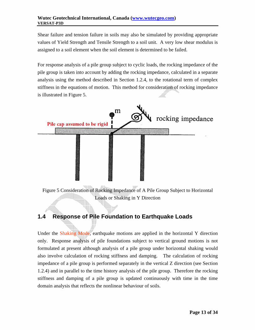
1.3 Response of Pile Foundation to Cyclic Loads..............................................................................12

1.4 Response of Pile Foundation to Earthquake Loads....................................................................13 1.4.1 Equations of Motion in Horizontal Y Direction .........................................................................14 1.4.2 Simulation of Soil Non-Linear Stress-Strain Response..............................................................14 1.4.3 Equivalent Viscous Damping......................................................................................................15 1.4.4 Consideration of Rocking Stiffness and Damping of Pile Group...............................................16

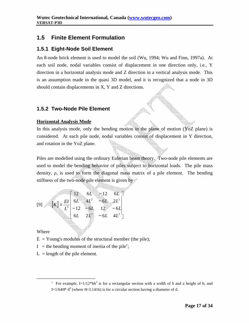
1.5 Finite Element Formulation..........................................................................................................17 1.5.1 Eight-Node Soil Element ............................................................................................................17 1.5.2 Two-Node Pile Element ..............................................................................................................17 1.5.3 Eight-Node (4-Beam) Pile Element ............................................................................................18 1.5.4 Batter Piles ..................................................................................................................................19

2.0 USERS MANUAL FOR VERSAT-P3D .................................................... 20

2.1 Input and Output Data Files .........................................................................................................20 2.1.1 For VERSAT-P3D Run...............................................................................................................20 2.1.2 Terminology in VERSAT-P3D Processor and PILE3D.P3D.....................................................20 2.1.3 Input Explanations for PILE3D.ATT..........................................................................................24

2.2 Prepare Input Data ........................................................................................................................25 2.2.1 Define 3D Grid in X-Y-Z and Soil Units in Z ............................................................................25 2.2.2 Define Piles for Location-Length and Pile Units........................................................................26 2.2.3 Define Properties of Pile and Soil Units .....................................................................................28 2.2.4 Define Control Parameters for Analysis .....................................................................................29 2.2.5 Define Parameters for Shaking Mode .........................................................................................30

2.3 Start An Analysis............................................................................................................................31

2.4 Retrieve Time-History Response ..................................................................................................31

3.0 EXAMPLES OF VERSAT-P3D MODELS................................................ 31

4.0 REFERENCES ......................................................................................... 34


Page 4 of 34

1.0 TECHNICAL MANUAL FOR VERSAT-P3D

1.1 Introduction In addition to the quasi-3D theory background as described in Wu and Finn (1997a, 1997b), a special 8-node (4-beam) pile element has been used in VERSAT-P3D. In addition to representing the pile by a line-beam element, which does not take a physical space in a 3D model, each pile segment can also be represented by four beams arranged at the four corners of a pile cross-section. For simplicity, a pile cross-section, either square or circular, is modeled as a square. The four beams are rigidly tied to each other so as to produce identical response, or to act as a single pile element. The 4-beam pile element is introduced to take into account the effect of the physical space of a pile section on the response of a single pile or a pile group. A VERSAT-P3D analysis can be carried out in one of the following three modes of analysis:

� Impedance Mode: Calculating dynamic stiffness and damping (impedance) in a frequency domain analysis;

� Loading Mode: Applying cyclic loads (shear forces and bending moments) at the pile head or at the pile cap in a frequency domain analysis; and

� Shaking Mode: Applying earthquake loads or dynamic loads at the pile head or at the pile cap in a time domain analysis.

The technical manual presents the theory and assumptions used in each of the above three modes of analyses.

a Wu, G., and Finn, W.D.L. 1997. Dynamic elastic analysis of pile foundations using finite element method in the frequency domain. Canadian Geotechnical Journal, 34: 34-43.

b Wu, G., and Finn, W.D.L. 1997. Dynamic nonlinear analysis of pile foundations using finite element method in the time domain. Canadian Geotechnical Journal, 34: 44-52.


Page 5 of 34

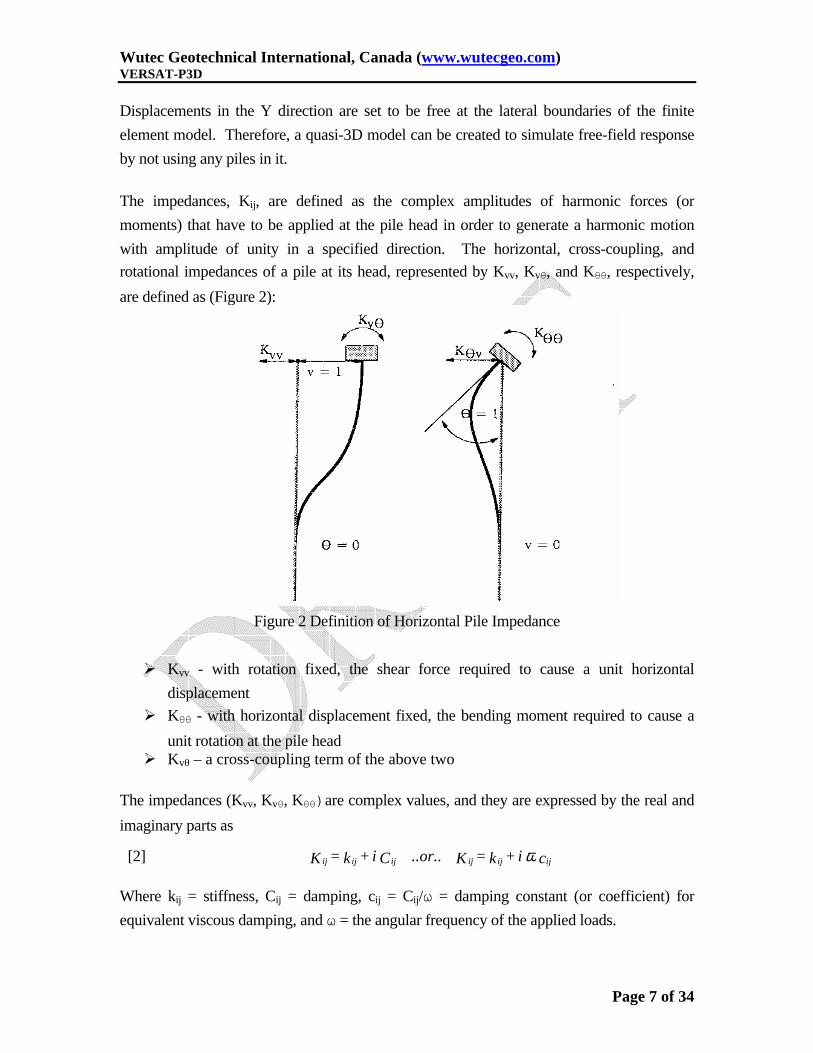
1.2 Dynamic Stiffness and Damping of Pile Foundation Under the Impedance Mode, dynamic stiffness and damping of pile foundations are obtained for the following

� Horizontal Y direction � Rotation about X axis (or in YoZ plane) � Coupling term of above two, and � Vertical Z direction

A separate model and thus a separate analysis will be required in order to compute horizontal and rotational stiffness and damping in the other horizontal direction, i.e., X direction. On the other hand, stiffness and damping for rotation about Z axis (or torsion) is not computed at present. If required, they need to be estimated from horizontal stiffness and damping.

1.2.1 Stiffness and Damping in Horizontal Direction

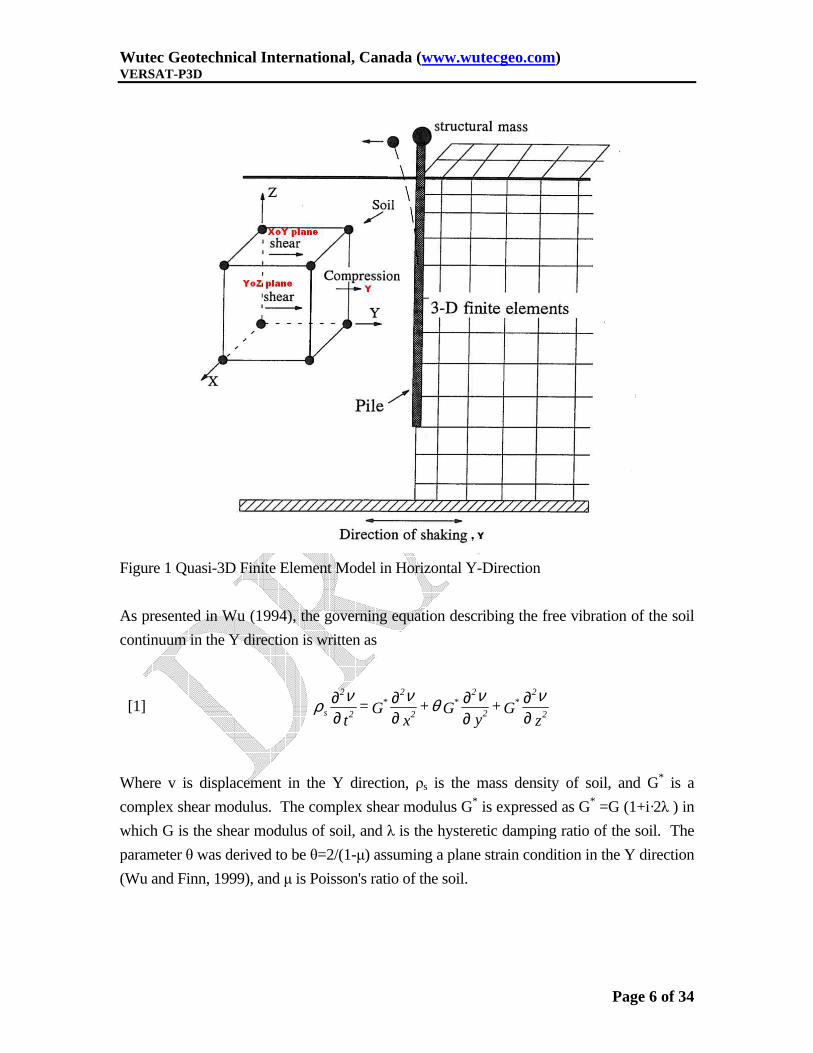
Subject to shear waves propagating in the vertical direction, the soils undergo mainly

shearing deformations in the horizontal (XoY) plane except in areas near the piles where

compression deformations develop in the direction of motion (Figure 1). The compressive

deformations also generate shearing deformations in YoZ plane. In the light of these

observations, assumptions are made that the dynamic motions are governed by shear waves

in the XoY and YoZ planes, and compression waves in the Y direction. Deformations in the

vertical direction and normal to the direction of motion are neglected to simplify a full 3D

analysis to a quasi 3D analysis. The quasi 3D analysis considers displacements in one

direction, Y, in a full 3D geometry.


Page 6 of 34

Figure 1 Quasi-3D Finite Element Model in Horizontal Y-Direction

As presented in Wu (1994), the governing equation describing the free vibration of the soil

continuum in the Y direction is written as

Where v is displacement in the Y direction, ρs is the mass density of soil, and G* is a

complex shear modulus. The complex shear modulus G* is expressed as G* =G (1+i·2λ ) in

which G is the shear modulus of soil, and λ is the hysteretic damping ratio of the soil. The

parameter θ was derived to be θ=2/(1-µ) assuming a plane strain condition in the Y direction

(Wu and Finn, 1999), and µ is Poisson's ratio of the soil.

[1] z

G + y

G + x

G = t 2

2*

2

2*

2

2*

2

2

s ∂∂

∂∂

∂∂

∂∂ ννθννρ


Page 7 of 34

Displacements in the Y direction are set to be free at the lateral boundaries of the finite

element model. Therefore, a quasi-3D model can be created to simulate free-field response

by not using any piles in it.

The impedances, Kij, are defined as the complex amplitudes of harmonic forces (or

moments) that have to be applied at the pile head in order to generate a harmonic motion

with amplitude of unity in a specified direction. The horizontal, cross-coupling, and

rotational impedances of a pile at its head, represented by Kvv, Kvθ, and Kθθ, respectively,

are defined as (Figure 2):

Figure 2 Definition of Horizontal Pile Impedance

� Kvv - with rotation fixed, the shear force required to cause a unit horizontal

displacement

� Kθθ - with horizontal displacement fixed, the bending moment required to cause a

unit rotation at the pile head � Kvθ – a cross-coupling term of the above two

The impedances (Kvv, Kvθ, Kθθ)are complex values, and they are expressed by the real and

imaginary parts as

Where kij = stiffness, Cij = damping, cij = Cij/ω = damping constant (or coefficient) for

equivalent viscous damping, and ω = the angular frequency of the applied loads.

[2] c i + k = K ..or.. C i + k = K ijijijijijij ω


Page 8 of 34

The hysteretic damping of soils is included in the complex shear modulus in Eq. [1]. The

radiation damping of a 3D geometry adopted in VERSAT-P3D consists of energy

dissipating boundaries including the horizontal base and the four vertical side surfaces.

1.2.2 Radiation Damping at Boundaries

The shear force caused by a particle velocity at the boundary is computed by

F = shear modulus (G) * particle velocity ÷ shear wave velocity (Vs) * area (dA)

With G = ρ Vs2, then

F = (ρ Vs dA) * particle velocity

Therefore, the damping matrix for an area in shearing is written as [3] cs = ∫A ρ Vs dA

Similarly the damping matrix for an area in compression is expressed as [4] cp = ∫A ρ Vp dA

Where Vp and Vs are the wave velocity in compression and in shearing. In VERSAT-P3D,

damping matrix is formed using the consistent formulation of above equations.

Under the shear wave in the Y direction, the horizontal base and the two vertical side

surfaces parallel to Y are assumed to be shearing boundary and the damping at these

surfaces is derived using Eq. [3]. The two vertical side surfaces parallel to X are assumed to

be in compression and the damping is derived using Eq. [4].

The energy transmitting boundary is applied only when the frequency of the loads is equal

to or greater than 3.14 rad/sec (or 0.5 Hz). Otherwise, static boundary conditions are

applied.

1.2.3 Stiffness and Damping in Vertical Direction

Subject to compression waves propagating in the vertical direction, the soil medium mainly

undergoes compressive deformations in the vertical direction, Z (Figure 3). In the two

horizontal directions, shearing deformations are generated due to the internal friction of the


Page 9 of 34

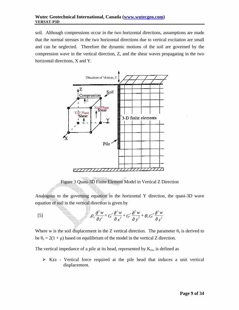
soil. Although compressions occur in the two horizontal directions, assumptions are made

that the normal stresses in the two horizontal directions due to vertical excitation are small

and can be neglected. Therefore the dynamic motions of the soil are governed by the

compression wave in the vertical direction, Z, and the shear waves propagating in the two

horizontal directions, X and Y.

Figure 3 Quasi-3D Finite Element Model in Vertical Z Direction

Analogous to the governing equation in the horizontal Y direction, the quasi-3D wave

equation of soil in the vertical direction is given by

Where w is the soil displacement in the Z vertical direction. The parameter θz is derived to

be θz = 2(1 + µ) based on equilibrium of the model in the vertical Z direction. The vertical impedance of a pile at its head, represented by Kzz, is defined as

� Kzz - Vertical force required at the pile head that induces a unit vertical displacement.

[5] z

wG +

y

wG +

x

wG =

t

w2

2*

z2

2*

2

2*

2

2

s ∂∂

∂∂

∂∂

∂∂ θρ


Page 10 of 34

The hysteretic damping of soils is included in the complex shear modulus in Eq. [5]. The

radiation damping of a 3D geometry adopted in VERSAT-P3D consists of energy

dissipating boundaries including the horizontal base and the four vertical side surfaces.

Under compression waves in vertical Z direction, the four vertical side surfaces parallel to Z

are assumed to be shearing boundary and the damping at these surfaces is derived using Eq.

[3]. The horizontal base is assumed to be in compression and the damping is derived using

Eq. [4].

Again, the energy transmitting boundary is applied only when the frequency of the loads is

equal to or greater than 3.14 rad/sec (or 0.5 Hz). Otherwise, static boundary conditions are

applied.

1.2.4 Stiffness and Damping of Pile Group in Rocking

The rocking impedance of a pile group is a measure of resistance to rotation of the pile cap

due only to the resistance of each pile in the group to vertical displacements. The rocking

impedance of a pile group, represented by Krr, is quantified as summation of moments of the

axial pile forces about the centre of rotation, Point O in Figure 4, induced by a unit rotation

about Point O. This definition is quantitatively expressed as

Where ri are distances between Point O and an individual pile in the group, and Fi are the

amplitudes of axial forces at the pile heads.

The rocking impedance, stiffness and damping, is computed assuming that piles located on

the right side of Point O (Figure 4) mirror the piles located on the left side of Point O. In

other words, only the piles on the left side of Point O are used in calculation, and the

computed rocking impedance is multiplied by two to derive the rocking impedance of the

pile group. This simplification only applies to calculation of rocking impedance. The

calculation of vertical impedance of a pile group uses all piles in a 3D model.

[6] F r = K iirr •Σ


Page 11 of 34

Figure 4 Calculation of Rocking Impedance in a Pile Group

The radiation damping in the calculation of rocking impedance takes the same form as in

the calculation of vertical impedance.

1.2.5 Stiffness and Damping of Pile Group in Translation & Rotation

Piles Fixed to the Pile Cap

For a pile group with piles fixed (rigidly connected) to the pile cap, the rotational

impedance of the pile group consists of two distinct components, the rotational

impedance of each individual pile and the rocking impedance of the pile group. In a

VERSAT-P3D calculation, the two components are computed separately. The rotational

impedances of individual piles in the group are computed using a quais-3D model in the

horizontal Y direction, and group effect is taken into account. The rocking impedance of

the pile group is computed using a quasi-3D model in the vertical Z direction, and group

effect is also taken into account.

The rotational impedance of the pile group is a summation of the two components. For

this condition, the horizontal displacement of the pile cap is coupled with rotation of the

pile cap.


Page 12 of 34

Piles Pinned to the Pile Cap

For a pile group with piles pinned to the pile cap, the rotational impedance of the pile

group consists of only the rocking impedance of the pile group. Rotational impedance of

individual piles does not provide resistance to rotation of the pile cap because the piles do

not carry bending moment at the pile head. The bending moment of the pile cap is

carried out by axial forces in the piles.

For this condition, the horizontal displacement of the pile cap is uncoupled with, or

independent to, the rotation of the pile cap, and the horizontal impedance of the pile

group is the so-called “apparent stiffness and damping” that represents the shear force

required to cause unit displacements when the pile head is free to rotation.

1.3 Response of Pile Foundation to Cyclic Loads

Under the Loading Mode, cyclic loads can be applied only in the horizontal Y direction.

Response to cyclic loads applied in the other horizontal X direction needs to be carried

out in a separate analysis. Analysis of response to cyclic loads in the vertical loads is not

available at present.

The steady-state response of pile foundation subject to cyclic loads (harmonic shear force

and/or bending moment) can be obtained by solving the equations of motion in the

frequency domain using the same method as for the calculation of impedance. However,

unlike in the impedance calculation where the analysis is linear elastic, the response

analysis can be done either in linear elastic or in nonlinear elastic.

For problems involving high magnitude of loads that can induce nonlinear response in

soils, the response to the cyclic loads will have to be computed using a method of

iteration to seek compatibility between magnitude of loads and stiffness of soils. In a

given iteration, the analysis is conducted as linear elastic. In a subsequent iteration of

analysis, the soil stiffness (or shear modulus to be specific) and damping are adjusted

based on the level of shear strain induced in the previous iteration. The relationships

between shear modulus, damping ratio and shear strain can be specified by the users.


Page 13 of 34

Shear failure and tension failure in soils may also be simulated by providing appropriate

values of Yield Strength and Tensile Strength to a soil unit. A very low shear modulus is

assigned to a soil element when the soil element is determined to be failed.

For response analysis of a pile group subject to cyclic loads, the rocking impedance of the

pile group is taken into account by adding the rocking impedance, calculated in a separate

analysis using the method described in Section 1.2.4, to the rotational term of complex

stiffness in the equations of motion. This method for consideration of rocking impedance

is illustrated in Figure 5.

Figure 5 Consideration of Rocking Impedance of A Pile Group Subject to Horizontal

Loads or Shaking in Y Direction

1.4 Response of Pile Foundation to Earthquake Loads

Under the Shaking Mode, earthquake motions are applied in the horizontal Y direction

only. Response analysis of pile foundations subject to vertical ground motions is not

formulated at present although analysis of a pile group under horizontal shaking would

also involve calculation of rocking stiffness and damping. The calculation of rocking

impedance of a pile group is performed separately in the vertical Z direction (see Section

1.2.4) and in parallel to the time history analysis of the pile group. Therefore the rocking

stiffness and damping of a pile group is updated continuously with time in the time

domain analysis that reflects the nonlinear behaviour of soils.


Page 14 of 34

1.4.1 Equations of Motion in Horizontal Y Direction

The governing equation of motion, Eq. [1], for quasi-3D analysis in the horizontal Y

direction, has been solved in the frequency domain for calculation of pile impedance and for

response analysis of pile foundations subject to cyclic loads at the pile head or the pile cap.

For response analysis of pile foundations subject to earthquake loads in the horizontal Y

direction, the governing equation of motion (Eq. [1]) will be solved in the time domain that

can simulate the time-dependent nonlinear behaviour of soils under earthquake shaking.

In a time domain analysis, the dynamic equilibrium equations of a soil-pile quasi-3D model

can be written in a matrix form as

in which ϋo(t) is the base accelerations, {I} is a unit column vector, and {ϋ} , { ύ} and {υ}

are nodal accelerations, velocities and displacements, respectively, relative to the model

base. [M], [C] and [K] are the mass, damping and stiffness matrices. Direct step-by-step

integration using the Wilson-θ method is used to solve the equations of motion in Eq. [7].

The non-linear hysteretic behaviour of the soil is modeled by using a variation of the

equivalent linear method similar to that used in the computer program SHAKE (Schnabel et

al., 1972). Additional features such as tension cut-off and yielding are also incorporated in

the program to simulate the possible gapping between soil and pile near the soil surface and

yielding in the near field.

1.4.2 Simulation of Soil Non-Linear Stress-Strain Response

An equivalent linear method is employed in the program to model the non-linear hysteretic

behaviour of soil. The basic assumption of this method is that the hysteretic behaviour of

soil can be approximated by a pair of secant shear moduli and viscous damping ratios which

are compatible with the level of shear strain. Typical relationships between shear modulus,

damping ratio and shear strain can be found in the literature such as Seed and Idriss (1970),

and Seed et al. (1986). This method has been accepted and widely used in engineering

practice, and it has been incorporated in the computer code SHAKE (Schnabel et al., 1972)

[7] (t)v[M]{I}- = [K]{v} + }v[C]{ + }v[M]{ 0&&&&&


Page 15 of 34

for 1-D ground motion analyses and in QUAD-4 (Idriss et al., 1973) for 2-D plane strain

analyses.

When the equivalent linear method is applied to earthquake problems involving irregular

amplitudes of shear strains with time, the current practice is to assign a constant effective

shear strain to a soil element to represent the variation of shear strains with time. The

effective shear strain is commonly taken as 65% of the maximum shear strain experienced

by the soil element during the life of earthquake shaking, and it is used to determine constant

effective G and λ of the soil element that are then used in the final iteration of analysis.

To approximate better the nonlinear behaviour of soil under strong shaking, compatibility

between secant shear modulus, damping ratio and shear strain should be sought at a time

interval within which the shear strain history can be suitably represented by a single value of

shear strain. This ensures that the time histories of shear moduli and damping ratios in each

soil element are followed during the analysis in contrast with the equivalent linear approach

described earlier in which a single effective value is used to represent the entire time history.

In a practical VERSAT-P3D analysis, the shear moduli and damping ratios are updated at

specified time intervals which balance accuracy and computational time. For the analyses

conducted to date using this method, it was found to be sufficient to update the soil

properties at every 0.5 to 1.0 sec based on the peak strain levels from the previous time

interval.

1.4.3 Equivalent Viscous Damping

The hysteretic damping ratio λ of soil is included in the dynamic analysis by using

equivalent viscous damping. A procedure for estimating viscous damping coefficients for

each individual element proposed by Idriss et al. (1974) is employed. The main advantage

of this procedure is that a different degree of damping can be applied in each finite element

according to its shear strain level. The damping is essentially of the Rayleigh-type, which is

both mass and stiffness dependent.


Page 16 of 34

The damping matrix [C]elem for a soil element is given by

Where ω1 is the fundamental frequency of the pile-soil system and is applied to each

element. The frequency ω1 is obtained by solving an eigen-value problem of the system and

is updated with time. The hysteretic damping ratio, λelem, is prescribed as a function of

element shear strain (Seed et al., 1986), and this is also time dependent.

The viscous damping as expressed in Eq. [8] provides a damping ratio of λelem at two

frequencies, one at ω1 and the other at four times ω1. At other frequencies, the damping

ratio could be either higher or lower than λelem.

1.4.4 Consideration of Rocking Stiffness and Damping of Pile Group

The rocking stiffness and damping constant of the pile group is taken into account by

adding them, calculated in a separate analysis using the method described in Section

1.2.3, to the rotational term of stiffness and damping constants in the equations of motion.

This method for the consideration of rocking impedance is illustrated in Figure 5.

[8] ) ][K + ][M ( = ][C elemelem1elemelem15

2

5

8

ωωλ


Page 17 of 34

1.5 Finite Element Formulation

1.5.1 Eight-Node Soil Element

An 8-node brick element is used to model the soil (Wu, 1994; Wu and Finn, 1997a). At

each soil node, nodal variables consist of displacement in one direction only, i.e., Y

direction in a horizontal analysis mode and Z direction in a vertical analysis mode. This

is an assumption made in the quasi 3D model, and it is recognized that a node in 3D

should contain displacements in X, Y and Z directions.

1.5.2 Two-Node Pile Element Horizontal Analysis Mode

In this analysis mode, only the bending motion in the plane of motion (YoZ plane) is

considered. At each pile node, nodal variables consist of displacement in Y direction,

and rotation in the YoZ plane.

Piles are modelled using the ordinary Eulerian beam theory. Two-node pile elements are

used to model the bending behavior of piles subject to horizontal loads. The pile mass

density, ρ, is used to form the diagonal mass matrix of a pile element. The bending

stiffness of the two-node pile element is given by

[9] [ ]

−−−−

−−

=

22

22

3

4626

612612

2646

612612

LLLL

LL

LLLL

LL

L

EIK

Where

E = Young's modulus of the structural member (the pile);

I = the bending moment of inertia of the pilec;

L = length of the pile element.

c For example, I=1/12*bh3 is for a rectangular section with a width of b and a height of h; and

I=1/64π* d4 (where π=3.1416) is for a circular section having a diameter of d.


Page 18 of 34

Vertical Analysis Mode

In the vertical analysis mode, variables of a pile node contain only displacement in the

vertical Z direction. The axial stiffness of the two-node pile element is given by

[10] L

EAK A =

Where:

A = sectional area of the pile (E, L are the same as in Eq. [9]).

1.5.3 Eight-Node (4-Beam) Pile Element

In short, the 8-node pile element takes the space as it is an 8-node soil element and it has the

properties of a 2-node beam element distributed into the eight pile nodes. In other words, a

pile segment is represented by four beams arranged at the four corners of the 8-node pile

element that represents the actual volume of the pile segment.

The purpose for using the 8-node pile element is to take into account the effect of pile

diameter on pile response. A 2-node pile element is a line-beam element that does not take

any physical space in a 3D model and therefore does not reflect the diameter effect on pile

behaviour. The use of one or multiple 8-node pile elements to represent a large-diameter

structure (such as a caisson, a vertical tunnel, or a shaft) section makes it possible to account

for the diameter effect on response.

When a structure section is represented by multiple 8-node pile elements, the geometric

properties (bending moment of inertia and section area) are evenly distributed to the number

of elements on the section. Of course, if one 8-node pile element is used, the actual

properties of the pile section are assigned to this pile element.

The procedure for such a representation has been verified by analyzing a vertical caisson

itself without any soil elements surrounding it. It is strongly recommended that the

behaviour of such a structural section of multiple 8-node elements be tested thoroughly prior

to applying it to a soil-structure interaction analysis.


Page 19 of 34

1.5.4 Batter Piles

Batter piles are approximately represented by modifying the horizontal stiffness of piles in a

horizontal analysis, and the vertical stiffness of piles in a vertical analysis mode.

The horizontal stiffness of a pile element in Eq. [9] is modified as

[11] αα 223

sincos12

aahori L

EA

L

EIK +=

Where α = the inclination angle to Z axis of the pile projected in YoZ plane, and

The rotational stiffness of the pile element is Eq. [9] is not affected by the batter.

The vertical stiffness of a pile element in Eq. [10] is modified as

[12] ββ 223

cossin12

aavert L

EA

L

EIK +=

Where β = the inclination angle of the pile to Z axis.

La = actual pile length of the batter pile along its axis.

The calculation of pile stiffness is taken care of by the program once the angles of

inclination, α and β, are entered for a pile.

The accuracy of the representation for batter piles is limited to the assumptions made above

in associated with the angle of pile inclination. It is recommended that the approximation be

used for piles with batter angle less than 30°.


Page 20 of 34

2.0 USERS MANUAL FOR VERSAT-P3D

2.1 Input and Output Data Files

2.1.1 For VERSAT-P3D Run The Windows-based interactive program, VERSAT-P3D Processor, is used to prepare and save the input data file for the computing program, VERSAT-P3D Run. Depending on the problem at hand, one to two input data files are required:

� PILE3D.P3D: Main input file required by all analyses. When the Shaking Mode is run, the earthquake accelerations are appended at the end of this file manually;

� PILE3D.ATT: This file is required in a nonlinear analysis. It contains data describing nonlinear relationships between shear modulus, material damping, and shear strains. Some published data are compiled and included in this that is distributed.

The results of the analysis are contained in three output data files:

� PILE3D.OU1 This file contains echo of model data and computed stiffness and damping values.

� PILE3D.OU2 This file contains printed node and element response. Under Loading Mode, the response is in complex value and contains real and imaginary parts. Under Shaking Mode, the response is in real value.

� PILE3D.HIS This file contains time-history response of the finite nodes and elements that are requested by the users. The data can be retrieved using a support program, V-HIS3D.exe.

VERSAT-P3D always uses the above names as data files for input and output.

2.1.2 Terminology in VERSAT-P3D Processor and PILE3D.P3D TITLE Title of the problem IMODE: Analysis mode including one of the three modes:

� Impedance Mode: impedance calculation (frequency domain analysis); � Loading Mode: harmonic loads at pile top/cap (frequency domain

analysis); and � Shaking Mode: earthquake loads or loads at pile top/cap (time

domain analysis). KIMP Index for computing impedance with a value of Yes or No ICHANG Method of analysis (linear elastic or nonlinear or equivalent linear) IROCK Pile head/cap condition using one of the three conditions:

� piles are pinned to the cap and moments at pile heads=0; � piles are fixed to the cap; and � piles are fixed to the cap and rotation of the cap is zero.


Page 21 of 34

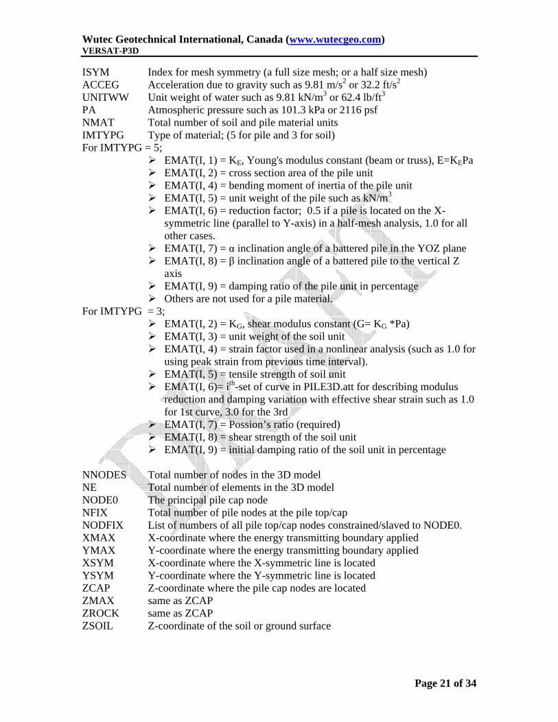
ISYM Index for mesh symmetry (a full size mesh; or a half size mesh) ACCEG Acceleration due to gravity such as 9.81 m/s2 or 32.2 ft/s2 UNITWW Unit weight of water such as 9.81 kN/m3 or 62.4 lb/ft3 PA Atmospheric pressure such as 101.3 kPa or 2116 psf NMAT Total number of soil and pile material units IMTYPG Type of material; (5 for pile and 3 for soil) For IMTYPG = 5;

� EMAT(I, 1) = KE, Young's modulus constant (beam or truss), E=KEPa � EMAT(I, 2) = cross section area of the pile unit � EMAT(I, 4) = bending moment of inertia of the pile unit � EMAT(I, 5) = unit weight of the pile such as kN/m3 � EMAT(I, 6) = reduction factor; 0.5 if a pile is located on the X-

symmetric line (parallel to Y-axis) in a half-mesh analysis, 1.0 for all other cases.

� EMAT(I, 7) = α inclination angle of a battered pile in the YOZ plane � EMAT(I, 8) = β inclination angle of a battered pile to the vertical Z

axis � EMAT(I, 9) = damping ratio of the pile unit in percentage � Others are not used for a pile material.

For IMTYPG = 3; � EMAT(I, 2) = KG, shear modulus constant (G= KG *Pa) � EMAT(I, 3) = unit weight of the soil unit � EMAT(I, 4) = strain factor used in a nonlinear analysis (such as 1.0 for

using peak strain from previous time interval). � EMAT(I, 5) = tensile strength of soil unit � EMAT(I, 6)= ith-set of curve in PILE3D.att for describing modulus

reduction and damping variation with effective shear strain such as 1.0 for 1st curve, 3.0 for the 3rd

� EMAT(I, 7) = Possion’s ratio (required) � EMAT(I, 8) = shear strength of the soil unit � EMAT(I, 9) = initial damping ratio of the soil unit in percentage

NNODES Total number of nodes in the 3D model NE Total number of elements in the 3D model NODE0 The principal pile cap node NFIX Total number of pile nodes at the pile top/cap NODFIX List of numbers of all pile top/cap nodes constrained/slaved to NODE0. XMAX X-coordinate where the energy transmitting boundary applied YMAX Y-coordinate where the energy transmitting boundary applied XSYM X-coordinate where the X-symmetric line is located YSYM Y-coordinate where the Y-symmetric line is located ZCAP Z-coordinate where the pile cap nodes are located ZMAX same as ZCAP ZROCK same as ZCAP ZSOIL Z-coordinate of the soil or ground surface


Page 22 of 34

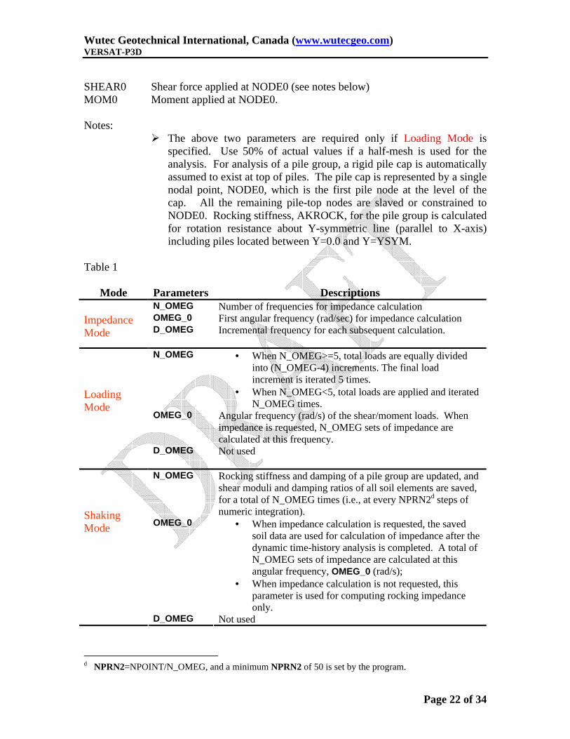
SHEAR0 Shear force applied at NODE0 (see notes below) MOM0 Moment applied at NODE0. Notes:

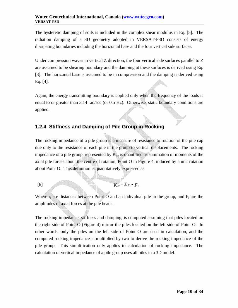
� The above two parameters are required only if Loading Mode is specified. Use 50% of actual values if a half-mesh is used for the analysis. For analysis of a pile group, a rigid pile cap is automatically assumed to exist at top of piles. The pile cap is represented by a single nodal point, NODE0, which is the first pile node at the level of the cap. All the remaining pile-top nodes are slaved or constrained to NODE0. Rocking stiffness, AKROCK, for the pile group is calculated for rotation resistance about Y-symmetric line (parallel to X-axis) including piles located between Y=0.0 and Y=YSYM.

Table 1

Mode Parameters Descriptions N_OMEG Number of frequencies for impedance calculation OMEG_0 First angular frequency (rad/sec) for impedance calculation

Impedance Mode D_OMEG Incremental frequency for each subsequent calculation.

N_OMEG • When N_OMEG>=5, total loads are equally divided

into (N_OMEG-4) increments. The final load increment is iterated 5 times.

• When N_OMEG<5, total loads are applied and iterated N_OMEG times.

OMEG_0 Angular frequency (rad/s) of the shear/moment loads. When impedance is requested, N_OMEG sets of impedance are calculated at this frequency.

Loading Mode

D_OMEG Not used

N_OMEG Rocking stiffness and damping of a pile group are updated, and shear moduli and damping ratios of all soil elements are saved, for a total of N_OMEG times (i.e., at every NPRN2d steps of numeric integration).

OMEG_0 • When impedance calculation is requested, the saved soil data are used for calculation of impedance after the dynamic time-history analysis is completed. A total of N_OMEG sets of impedance are calculated at this angular frequency, OMEG_0 (rad/s);

• When impedance calculation is not requested, this parameter is used for computing rocking impedance only.

Shaking Mode

D_OMEG Not used

d NPRN2=NPOINT/N_OMEG, and a minimum NPRN2 of 50 is set by the program.


Page 23 of 34

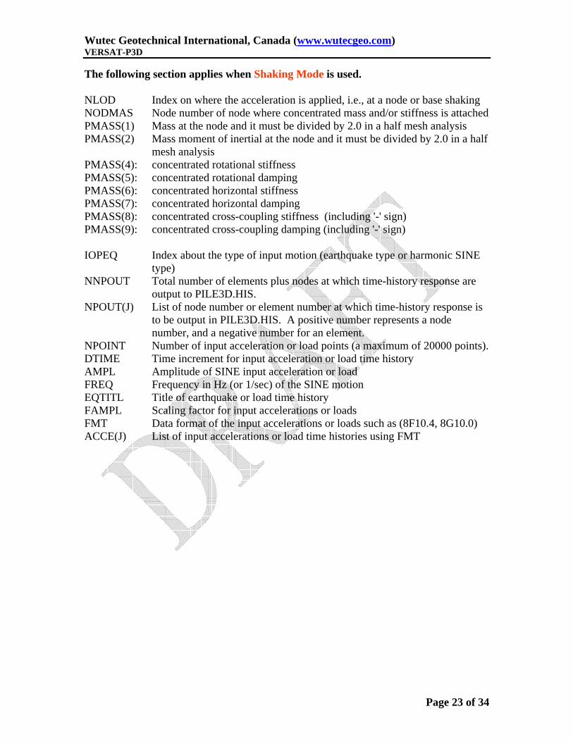
The following section applies when Shaking Mode is used. NLOD Index on where the acceleration is applied, i.e., at a node or base shaking NODMAS Node number of node where concentrated mass and/or stiffness is attached PMASS(1) Mass at the node and it must be divided by 2.0 in a half mesh analysis PMASS(2) Mass moment of inertial at the node and it must be divided by 2.0 in a half

mesh analysis PMASS(4): concentrated rotational stiffness PMASS(5): concentrated rotational damping PMASS(6): concentrated horizontal stiffness PMASS(7): concentrated horizontal damping PMASS(8): concentrated cross-coupling stiffness (including '-' sign) PMASS(9): concentrated cross-coupling damping (including '-' sign)

IOPEQ Index about the type of input motion (earthquake type or harmonic SINE

type) NNPOUT Total number of elements plus nodes at which time-history response are

output to PILE3D.HIS. NPOUT(J) List of node number or element number at which time-history response is

to be output in PILE3D.HIS. A positive number represents a node number, and a negative number for an element.

NPOINT Number of input acceleration or load points (a maximum of 20000 points). DTIME Time increment for input acceleration or load time history AMPL Amplitude of SINE input acceleration or load FREQ Frequency in Hz (or 1/sec) of the SINE motion EQTITL Title of earthquake or load time history FAMPL Scaling factor for input accelerations or loads FMT Data format of the input accelerations or loads such as (8F10.4, 8G10.0) ACCE(J) List of input accelerations or load time histories using FMT


Page 24 of 34

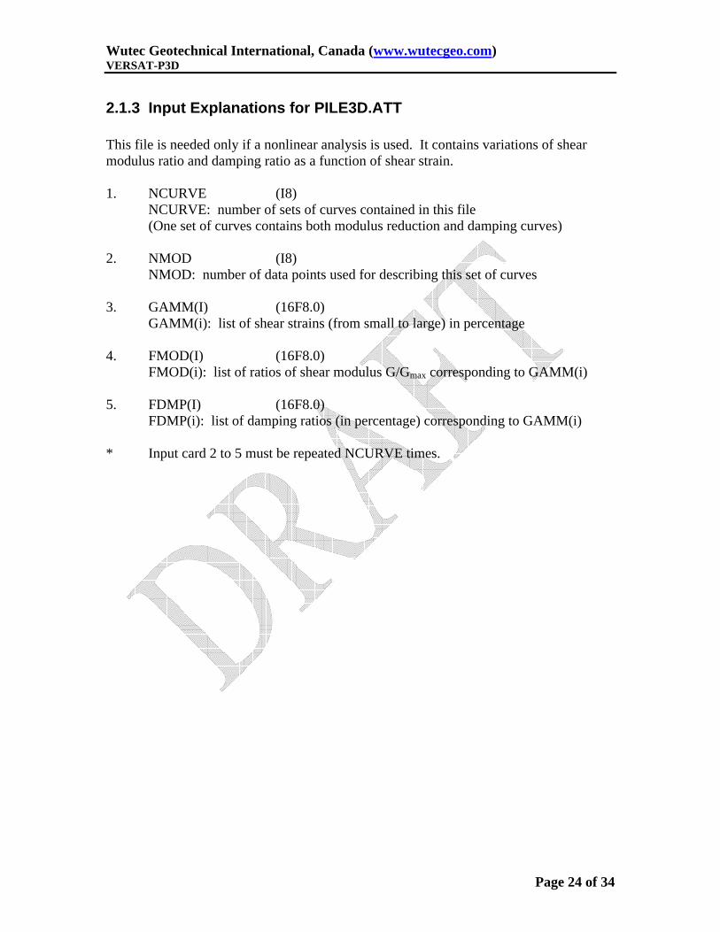
2.1.3 Input Explanations for PILE3D.ATT This file is needed only if a nonlinear analysis is used. It contains variations of shear modulus ratio and damping ratio as a function of shear strain. 1. NCURVE (I8)

NCURVE: number of sets of curves contained in this file (One set of curves contains both modulus reduction and damping curves)

2. NMOD (I8)

NMOD: number of data points used for describing this set of curves 3. GAMM(I) (16F8.0)

GAMM(i): list of shear strains (from small to large) in percentage 4. FMOD(I) (16F8.0)

FMOD(i): list of ratios of shear modulus G/Gmax corresponding to GAMM(i) 5. FDMP(I) (16F8.0)

FDMP(i): list of damping ratios (in percentage) corresponding to GAMM(i)

* Input card 2 to 5 must be repeated NCURVE times.


Page 25 of 34

2.2 Prepare Input Data

2.2.1 Define 3D Grid in X-Y-Z and Soil Units in Z

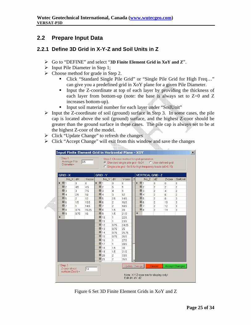
� Go to “DEFINE” and select “3D Finite Element Grid in XoY and Z”. � Input Pile Diameter in Step 1; � Choose method for grade in Step 2.

� Click “Standard Single Pile Grid” or “Single Pile Grid for High Freq…” can give you a predefined grid in XoY plane for a given Pile Diameter.

� Input the Z-coordinate at top of each layer by providing the thickness of each layer from bottom-up (note: the base is always set to Z=0 and Z increases bottom-up).

� Input soil material number for each layer under “SoilUnit” � Input the Z-coordinate of soil (ground) surface in Step 3. In some cases, the pile

cap is located above the soil (ground) surface, and the highest Z-coor should be greater than the ground surface in these cases. The pile cap is always set to be at the highest Z-coor of the model.

� Click “Update Change” to refresh the changes � Click “Accept Change” will exit from this window and save the changes

Figure 6 Set 3D Finite Element Grids in XoY and Z


Page 26 of 34

2.2.2 Define Piles for Location-Length and Pile Units

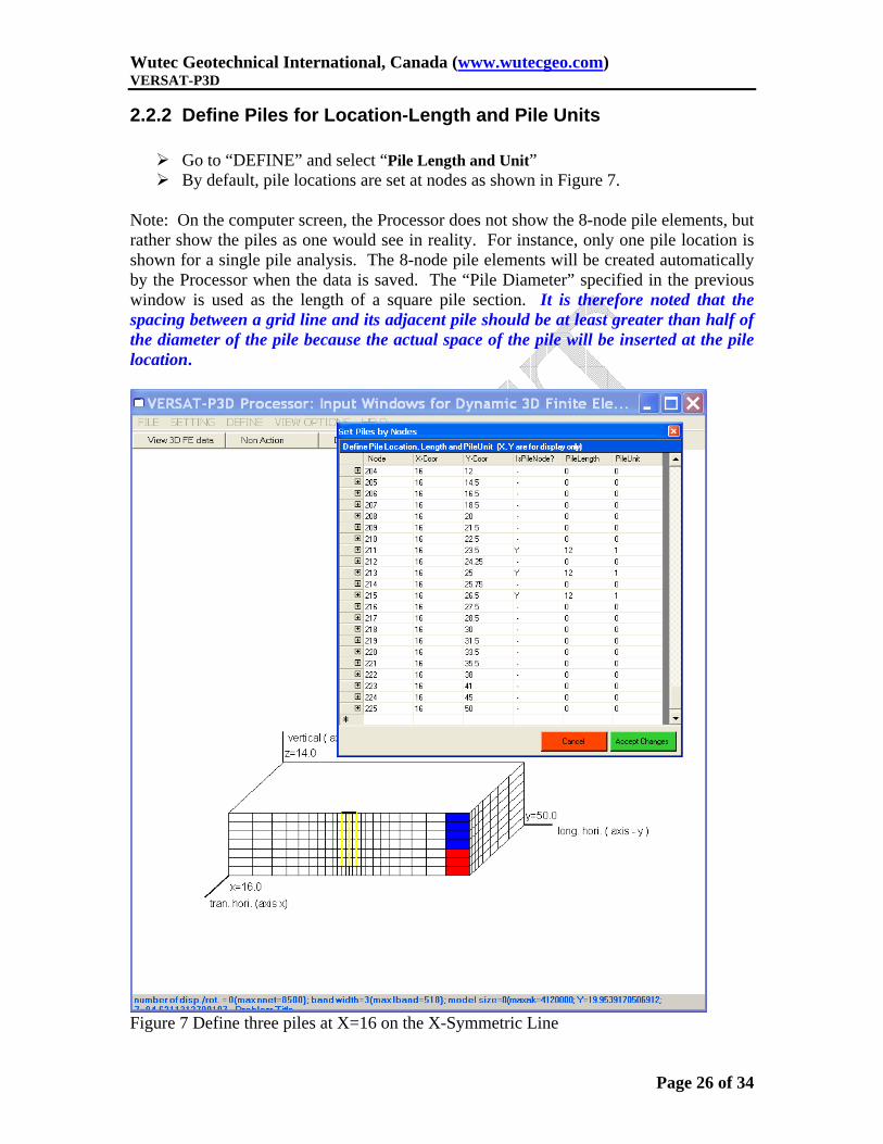
� Go to “DEFINE” and select “Pile Length and Unit” � By default, pile locations are set at nodes as shown in Figure 7.

Note: On the computer screen, the Processor does not show the 8-node pile elements, but rather show the piles as one would see in reality. For instance, only one pile location is shown for a single pile analysis. The 8-node pile elements will be created automatically by the Processor when the data is saved. The “Pile Diameter” specified in the previous window is used as the length of a square pile section. It is therefore noted that the spacing between a grid line and its adjacent pile should be at least greater than half of the diameter of the pile because the actual space of the pile will be inserted at the pile location.

Figure 7 Define three piles at X=16 on the X-Symmetric Line


Page 27 of 34

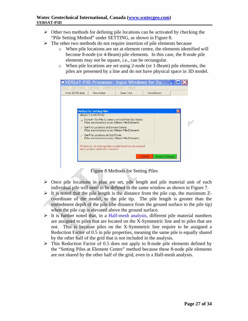
� Other two methods for defining pile locations can be activated by checking the “Pile Setting Method” under SETTING, as shown in Figure 8.

� The other two methods do not require insertion of pile elements because o When pile locations are set at element centre, the elements identified will

become 8-node (or 4-Beam) pile elements. In this case, the 8-node pile elements may not be square, i.e., can be rectangular.

o When pile locations are set using 2-node (or 1-Beam) pile elements, the piles are presented by a line and do not have physical space in 3D model.

Figure 8 Methods for Setting Piles

� Once pile locations in plan are set, pile length and pile material unit of each

individual pile will need to be defined in the same window as shown in Figure 7. � It is noted that the pile length is the distance from the pile cap, the maximum Z-

coordinate of the model, to the pile tip. The pile length is greater than the embedment depth of the pile (the distance from the ground surface to the pile tip) when the pile cap is elevated above the ground surface.

� It is further noted that, in a Half-mesh analysis, different pile material numbers are assigned to piles that are located on the X-Symmetric line and to piles that are not. This is because piles on the X-Symmetric line require to be assigned a Reduction Factor of 0.5 in pile properties, meaning the same pile is equally shared by the other half of the grid that is not included in the analysis.

� This Reduction Factor of 0.5 does not apply to 8-node pile elements defined by the “Setting Piles at Element Centre” method because these 8-node pile elements are not shared by the other half of the grid, even in a Half-mesh analysis.


Page 28 of 34

2.2.3 Define Properties of Pile and Soil Units

� Go to DEFINE and select “Pile and Soil Properties” � For the example being illustrated, Unit 1 is assigned to the three piles on the X-

Symmetric line and thus has a Reduction Factor of 0.5. Units 2 and 3 are assigned to the two soil units, the red and the blue zones shown on the vertical grids. Unit 4 is assigned to a Reduction Factor of 1.0 and other properties same as Unit 1, and it can be assigned to piles located not on the X-Symmetric line. Unit 4 is not used in this example.

� It is noted that the total unit weight should be assigned to piles and soils although they may be submerged.

Figure 9 Assign Properties of Pile and Soil Units


Page 29 of 34

2.2.4 Define Control Parameters for Analysis

� Go to DEFINE and select “Control Parameters”. This window will define what analysis will be carried out and how it is carried out.

� Figure 10 shows parameters under the Loading Mode. A combination of cyclic shear and moment (shear force=200 kN and bending moments=500 kN.m) is applied at the pile cap in a Half-mesh analysis while the piles are fixed to the pile cap. Note that “Shear of 100 and Moments of 250” are entered in the window. The frequency of the cyclic loads is 1 Hz (6.28 rad/sec). The loads will be divided into 6 increments and applied incrementally in a nonlinear analysis. A total of 10 analyses will be performed with the last load increment being iterated 5 times.

Figure 10 Define Parameters under Loading Mode


Page 30 of 34

2.2.5 Define Parameters for Shaking Mode

� In Figure 10, click Shaking Mode under “Analysis Mode” � Go to DEFINE and select “Setup for Shaking Mode” � In Figure 11, an acceleration record from the 1971 San Fernando Earthquake will

be appended MANUALLY by the user at the end of PILE3D.P3D. The record is written in 8 columns with a comma separating two columns. The first 2000 acceleration points from the record will be used in the dynamic analysis. The time increment for the record is 0.02 sec, and the acceleration values will be multiplied by 9.81 to convert into the unit of m/s2 for accelerations to be used in the analysis (assuming the original values are in g).

� Time-histories response at node 500 and element 200 will be saved under PILE3D.HIS.

� No external mass or stiffness is applied at the pile cap (all zero in entries).

Figure 11 Define Parameters under Shaking Mode


Page 31 of 34

2.3 Start An Analysis

� Save the prepared data as PILE3D.P3D � Re-load the saved data back. The Processor can then verify the size of the model

being less than the maximum allowed size, and show the node and element information of the 3D model. Without a reloading, these data are not available.

� Run VERSAT-P3D Run.exe under either Windows or Dos environment. Make sure that PILE3D.P3D is under the same directory as VERSAT-P3D Run.exe.

2.4 Retrieve Time-History Response A separate computer program, called V-his3d.exe, is used to retrieve the time-history from PILE3D.HIS, a binary file containing time-history response. Another input file to V-his3d.exe is PILE3D.IN . An example of PILE3D.IN, containing only two lines, is as follows:

Line 1: 4, 0, 0, Line 2: 1, 2, 3, 4,

Line 1:

NDATA Total number of time-histories is requested; N1 0, always N2 0, not used

Line 2:

List of codes representing the specific quantity (such as acceleration, displacement, bending moment, shear force, etc.). These codes for retrieving a time-history response at a node or in an element are printed at the end of the output file, PILE3D.OU2.

3.0 EXAMPLES OF VERSAT-P3D MODELS The example models shown in Figure 12 include the following:

� a). Structural analysis of vertical caissons only � b). Analysis of free field response using a 10-layer model � c). Analysis of a 12-pile group (shown as 8-pile group in a half-mesh analysis)

with an elevated pile cap � d). Analysis of a large 44-pile group (shown as 24-pile in a half-mesh analysis)

Analyses of these models are tasks for the users to complete..


Page 32 of 34

a). Structural analysis of vertical caissons only

b). Analysis of free field response using a 10--layer model

c). VERSAT-P3D Model for analysis of 12-pile group (shown as 8-pile group in a half-mesh analysis) with an elevated pile cap


Page 33 of 34

d). VERSAT-P3D model for analysis of a large 44-pile group (shown as 24-pile in a half-mesh analysis)

Figure 12 Examples of VERSAT-P3D Models


Page 34 of 34

4.0 REFERENCES

Idriss, I.M., Lysmer, J., Hwang, R., and Seed, H.B. 1973. QUAD-4: A computer program

for evaluating the seismic response of soil-structures by variable damping finite element

procedures. Report No. EERC 73-16, Earthquake Engineering Research Centre, University

of California, Berkeley, California.

Idriss, I.M., Seed, H.B., and Serff, N. 1974. Seismic response by variable damping finite

elements. ASCE Journal of Geotechnical Engineering, 100: 1-13.

Schnabel, P.B., Lysmer, J., and Seed, H.B. 1972. SHAKE: A computer program for

earthquake response analysis of horizontally layered sites. Report No. EERC 72 12,

Earthquake Engineering Research Centre, University of California, Berkeley, California.

Seed, H.B., and Idriss, I.M. 1970. Soil moduli and damping factors for dynamic response

analyses. Report No. ERRC 70 10, Earthquake Engineering Research Center, University of

California, Berkeley, California.

Seed, H.B., Wong, R.T., Idriss, I.M., and Tokimatsu, K. 1986. Moduli and damping factors

for dynamic analyses of cohesionless soils. ASCE Journal of Geotechnical Engineering,

112: 1016 1032.

Wu, G. 1994. Dynamic soil-structure interaction: Pile foundations and retaining structures.

Ph.D. thesis, Department of Civil Engineering, the University of British Columbia,

Vancouver, B.C., Canada.

Wu, G., and Finn, W.D.L. 1997a. Dynamic elastic analysis of pile foundations using finite

element method in the frequency domain. Canadian Geotechnical Journal, 34: 34-43.

Wu, G., and Finn, W.D.L. 1997b. Dynamic nonlinear analysis of pile foundations using

finite element method in the time domain. Canadian Geotechnical Journal, 34: 44-52. Wu, G. and W.D.L. Finn, 1999. Seismic lateral pressures for design of rigid walls. Canadian Geotechnical Journal, 36: 509 - 522

Date post:	05-Mar-2018
Category:	Documents
Upload:	phungkiet
View:	226 times
Download:	4 times

VERSAT – P3D Version 2006 QUASI-3D DYNAMIC FINITE ELEMENT ... version2006.pdf · QUASI-3D DYNAMIC...

Documents