1 Vertical Axis Wind Turbine development Guilherme Silva Abstract: Wind power is, nowadays, the most promising and suitable renewable energy for rapid and cost-effective implementation. Horizontal axis wind turbines have been greatly developed but some other technologies, such as the vertical axis wind turbines are still in an initial development phase. The disparity in the development of these technologies remains unexplained. Nevertheless, the little development made in vertical axis wind turbines seems to emphasize this technology as being one of great potential. This present work aimed to create an analysis of this technology. Models were developed, and a wide range of CFD results were obtained using the kw SST model. In the end, a small wind turbine intentionally built for this work was tested. Keywords: VAWT Darrieus Giromill H-rotor Vertical axis wind turbine Wind power Kw model. ABBREVIATIONS AND ACRONYMS A Area; AR Aspect ratio; c Blade chord; D C Drag coefficient; L C Lift coefficient; P C Power coefficient; COE Cost of energy; D Drag; EU European Union; f Frequency; F Force; n F Lateral force; t F Tangential force; HAWT Horizontal axis wind turbine; I Moment of inertia; L Lift; LC Lifetime costs; LEO Lifetime energy output; M Torque; n Number of blades; P Power; r Radius; Re Reynolds number; t Time; V Velocity; VAWT Vertical axis wind turbine; in cut V _ Start-up velocity; out cut V _ Maximum velocity; i V Induced velocity; p V Blade’s flow velocity; rated V Nominal velocity; V Wind velocity; Angle of attack; Angular position; Tip speed ratio; Density; Solidity; Angular velocity; Kinematic viscosity. I. INTRODUCTION Wind energy is the energy from the wind. This form of energy can be converted to other more useful forms such as electricity, through the use of wind turbines. Wind power is the power, in W, given by the kinetic energy of wind in a given area, per unit of time [3] : 3 2 1 AV P wind , (1) being is the density of air in kg/m 3 , A the area considered in m 2 and V the wind velocity in m/s. Worldwide, the use of wind power has been rising, around 25% per year, since the early 1990s. This increase has been stronger in Europe. In the future, this trend is expected to continue mainly through the use of offshore areas [5] . The efficiency of wind turbines is normally characterized by the power coefficient [3] : 3 2 1 AV P P P C turbine wind turbine P . (2) Wind turbines can be divided into two types. In drag turbines, movement is produced by the air drag while in lift turbines movement is produced by the air lift in the turbine’s blades. One of the most important concepts of wind turbines is the tip speed ratio defined as V r , (3) being r the blade’s velocity in m/s and V the wind velocity in m/s [1] .
Transcript
1
Vertical Axis Wind Turbine development Guilherme Silva
Abstract: Wind power is, nowadays, the most promising and suitable renewable energy for rapid and cost-effective implementation. Horizontal axis wind turbines have been greatly developed but some other technologies, such as the vertical axis wind turbines are still in an initial development phase. The disparity in the development of these technologies remains unexplained. Nevertheless, the little development made in vertical axis wind turbines seems to emphasize this technology as being one of great potential. This present work aimed to create an analysis of this technology. Models were developed, and a wide range of CFD results were obtained using the kw SST model. In the end, a small wind turbine intentionally built for this work was tested.
Wind energy is the energy from the wind. This form of energy can be converted to other more useful forms such as electricity, through the use of wind turbines.
Wind power is the power, in W, given by the kinetic energy of wind in a given area, per unit of time
[3]:
3
2
1 AVPwind , (1)
being is the density of air in kg/m3, A the area
considered in m2 and V the wind velocity in m/s.
Worldwide, the use of wind power has been rising, around 25% per year, since the early 1990s. This increase has been stronger in Europe. In the future, this trend is expected to continue mainly through the use of offshore areas
[5].
The efficiency of wind turbines is normally characterized by the power coefficient
[3]:
3
2
1
AV
P
P
PC turbine
wind
turbineP
. (2)
Wind turbines can be divided into two types. In drag turbines, movement is produced by the air drag while in lift turbines movement is produced by the air lift in the turbine’s blades. One of the most important concepts of wind turbines is the tip speed ratio defined as
V
r , (3)
being r the blade’s velocity in m/s and V the wind
velocity in m/s[1]
.
2
In drag turbines, theoretically, 1 . Drag turbines also
tend to start movement at lower V but have high drag at
high V . On the other hand, lift turbines have starting
problems, usually needing help to start but have lower drag
at high V and usually superior PC [1].
Wind turbines can also be divided into HAWT (Horizontal Axis Wind Turbine) and VAWT (Vertical Axis Wind Turbine). VAWTs seem to have easier maintenance, less noise and do not need alignment with the wind
[1,3].
Many types of wind turbines have been developed as shown in Figure 1.
Figure 1 – Types of wind turbines
The most widely spread type of wind turbine is the 3-bladed HAWT, but other types have demonstrated good feasibility, such as the Darrieus or the giromill turbine. The giromill turbine, using untwisted straight blades allows an easier construction and transport, reducing costs
[1].
The Betz’s limit is the theoretical maximum PC value:
%5927
16max PC (4)
calculated assuming an ideal turbine, with infinite number of blades, without losses
[3].
II. WORKING PARAMETERS
Although giromill VAWTs are the simplest type of wind turbine, its aerodynamic analysis is very complex
[1]. Consider
a turbine with radius r , spinning at angular velocity
within a flow with velocity V . The blade’s wind velocity
pV can be decomposed into its normal component nV
(pointing from inside to outside the turbine) and its
tangential component tV (pointing from the leading edge to
the trailing edge):
)cos( VrVt , (5)
)(senVVn . (6)
With the increase of , tV becomes the dominant
component in pV , diminishing the blade’s angle of attack
[8]:
t
n
V
V1tan . (7)
Replacing in the previous formulas,
)cos(
)(tan 1 sen
. (8)
Graph 1 – α according to θ and λ
is independent of V and it varies less with
increase. For 3 , 20max .
pV is given by[8]
:
22
ntp VVV . (9)
Combining the previous formulas:
1cos22 VVp , (10)
12 VVp,
(11)
The mean Reynolds number can be obtained by
cV
1Re
2 . (12)
being c the blade’s chord in m and the kinematic
viscosity of air in m2/s. For a VAWT with 10c cm, with
8 and 11V m/s, 5106Re .
The resulting aerodynamic forces in the blades can be
obtained by the interpolation of LC and DC according to
the airfoil used and the given conditions of and Re . This
kind of information is hard to find for typical working
conditions of a VAWT (low Re and high )[2]
.
The blade’s force components can be obtained by[8]
:
cosDLsenFt , (13)
DsenLFn cos , (14)
as depicted in Figure 2.
-90-75-60-45-30-15
0153045607590
0 90 180 270 360
α ⁰
θ ⁰
1
2
3
4
5
6
7
λ
3
Figure 2 – VAWT’s aerodynamic forces
It can be concluded that has a primary importance in
the intensity of tF . As seen before, depends on . This
relationship defines the working conditions of the turbine.
At low , is high, making the blade stall, diminishing the
DL ratio. At high , is low and the tangential
component of L is small. There is an optimum where
is high enough for the tangential component of L to be
considerable and low enough for the DL ratio to be high.
For a VAWT, optimum is usually between 3 and 5[1]
.
According to these conclusions, an airfoil suitable for a giromill VAWT should stall at high , allowing its use at
high (low ), maximizing the tangential component of
L , increasing tF . On the other hand, the DL ratio
should be kept high to reduce the drag on each blade. A possible solution for both these restrictions would be the use of an airfoil with a drag bucket.
The power produced is obtained by[8]:
MP , (15)
rFnM t .
(16)
In the turbine’s blades, the quick change of and pV
makes the blade’s response dynamic, different from the results normally published in static regimes. That difference is important and depends on many factors. In these conditions, stall is denominated dynamic stall. In VAWTs, dynamic stall has been found to provide higher efficiency but also higher noise and fatigue
[2].
Parashivoiu[1]
concluded that there is no advantage in a bigger diameter, as the turbine’s cost increases with the cube of the diameter while the energy captured increases
with the square of the diameter (for 1AR ).
The increase of AR , increases and diminishes M (for
the same amount of turbineP ). These parameters should be
set according to the type of generator used. As generators
tend to work at high , high AR turbines (high ) are
suitable for a direct connection to the generator while low
AR turbines (with low but high M ) should use a
gearbox. High AR increases the amount of material and the area of the blades (a costly component). Equilibrium must be found between cost and efficiency
[1].
End/tip losses occur due to the flow from the highest pressure to the lowest pressure side of the blade’s tip. This
effect is attenuated by the use of high AR or wingtips. This is the main factor indicated as responsible for the differences between 2D and 3D simulations of a VAWT’s flow
[10].
Solidity is a crucial parameter in VAWT development and is obtained by:
rnc (17)
Results indicate that lower results in higher efficiency
and optimum [1].
For a given is structurally more advantageous to have
fewer blades with higher c [1]. But 3-bladed turbines have a
more stable operation than 2-bladed turbines. This happens because the resulting aerodynamic forces at the blades reach maximum at each half turn. With two blades, these maximums are reached in phase
[2].
With the adequate roughness, it is possible to force the transition of a laminar boundary layer to turbulent. In VAWT, blade’s roughness is an important parameter
[10].
The airfoils usually studied have been developed for the aircraft industry. For VAWTs, the working regimes are
different, namely with higher and lower Re . This makes
the usual studied airfoils ill-fitted for VAWTs[1-3]
. It was demonstrated that for the NACA 4 digits airfoils, using airfoils with higher thickness (over 18%) increased performance
[1].
It was thought that the use of airfoils with camber would not be successful because as changes sign each half turn,
any gain obtained with positive would be lost when
was negative. The Sandia laboratories and Kirke[2]
tested VAWTs equipped with cambered airfoils and concluded that
the use of cambered airfoils had increased maxPC and
optimum [1].
One greatest disadvantage of lift VAWTs is the usual lack of automatic start-up. Many solutions have been presented, most commonly the use of drag elements, obtaining a hybrid lift-drag VAWT. According to Kirke
[2], on the other hand, drag
elements with an area lower than 10% of the VAWT’s area
4
have little effect. He also says that the more viable current solutions are the use of cambered airfoils, flexible blades or passive pitch control techniques.
III. SIMILAR SYSTEMS
Data from small commercially available VAWTs was obtained based from reference [13]. This data was compiled in a database used to evaluate important parameters in the development of VAWTs.
VAWTs usually indicate the nominal power, produced at
ratedV . ratedV is usually high (10-16m/s) making the values
presented inappropriate for most locations. The correct method for estimating energy production is by analyzing the probability distribution of wind speed and the power curve of the turbine.
To compare different parameters amongst VAWTs according to power developed, it is important to set a common condition for power production. This condition was
set as 5V m/s. Nominal power was compared to power
produced at 5V m/s (Graph 2).
Graph 2 – Power produced at V∞=5m/s vs nominal power
The cost of VAWTs was compared as shown in Graph 3.
Graph 3 – Price according to power produced at V∞=5m/s
The values obtained depend on many factors such as location, transport, taxes, warranties, etc. For the database, the values present the cost of the complete VAWT, in the place of production (no transport or assembly). There is a wide range of values, explained by the differences in the product’s quality and the fact that this is a recent and growing market where competition needs to settle.
To analyze the A and AR of the VAWTs, Graph 4, Graph 5 and Graph 6 were obtained.
Graph 4 – Price vs area
Graph 5 – Power produced at V∞=5m/s vs area
Graph 6 – AR analysis of VAWTs
The small range of areas compiled does not allow a complete analysis of the price evolution according to the area. Graph 6 presents the results of 42 VAWTs with full
lines representing the area and dotted lines the AR .
Though VAWTs with 1AR are 2/3 of the total, there are
many VAWTs with low AR . This parameter is mainly associated with the type of generator used, as explained before. From the analyzed VAWTs, most use a direct drive, permanent magnet generator developed intentionally. The number of blades varies between 3 and 5, 5 being the most common value.
IV. AERODYNAMIC ANALYSIS
A. State of the art
Nowadays a complete theoretical procedure for the development of a VAWT does not exist. Most development
y = 0,07x + 24
0
100
200
300
400
500
600
0 1000 2000 3000 4000 5000 6000
Po
we
r w
ith
win
d s
pe
ed
of
5m
/s
W
Nominal power W
y = 16x + 5292
0
5000
10000
15000
20000
25000
0 100 200 300 400 500 600
Pri
ce
€
Power with wind speed of 5m/s W
y = 1295x + 1918
0
10000
20000
30000
0 5 10 15 20
Pri
ce
€
Area m²
y = 25x + 42
0
100
200
300
400
500
600
0 5 10 15 20
Po
we
r w
ith
win
d s
pe
ed
of
5m
/s
W
Area m²
0
1
2
3
4
5
6
7
8
0 2 4 6 8
He
igh
t
m
Diameter m
Max for 5
m/s
AR=2 AR=1
AR=0,5
AR=3
AR=0,33
A=2m2
A=6m2
A=16m2
5
is done by obtaining results for many configurations by numerical computation
[1]. Many aerodynamic models have
been developed for VAWTs such as the double/multiple streamtube model, the vortex model and the cascade model. These models usually contain various components, developed in the following order:
Calculation of pV , according to , , r and V ;
Calculation of the aerodynamic forces applied in the blades;
Calculation of the VAWT induced velocity (different from the airflow’s speed due to the interaction of the turbine over the flow);
Calculation of tridimensional effects;
Consideration of dynamic stall[1,8]
.
Computational fluid dynamics has been used with success for wind turbines. Although at the cost of great computational effort, CFD is able to simulate dynamic stall. The results obtained depend on the model used, the mesh parameters and the convergence criteria
[1]. 3D CFD of
VAWTs requires, at least, 30 times more computational capacity than 2D simulations.
[14].
Wang[15]
, used the kw SST model to study a giromill VAWT and concluded that this model provides results similar to experimental data. He also concluded that for the simulation of giromill VAWTs, the kw SST transitional model should be preferred to models ke, Spalart-Allmaras or Baldwin-Lomax. Howell
[10] indicates that the CFD ke standard model has low
accuracy results.
B. Analysis made
Results were obtained using CFD. The kw SST transitional model was chosen given the good results previously obtained by investigators of IST and Wang
[15]. The results
were obtained for a VAWT giromill similar to the prototype that would later be developed. The prototype is small to reduce costs, building time and to facilitate testing. The VAWT simulated has r=0,5m, the c=5 or 10cm long. The number of blades varies between 2 and 5. The airfoils used are the NACA0012 and NACA0018 due to the extensive information available and the recommendation from IST investigators. Using these parameters, 7 configurations were tested as shown in Table 1 .
Configuration Airfoil c mm n σ
1
NACA0018
50
3 0,3
2 2 0,2
3 4 0,4
4 100
2 0,4
5 3 0,6
6 50
5 0,5
7 NACA0012 3 0,3
Table 1 – Configurations analyzed with CFD
The configurations were chosen to allow the study of
different parameters such as AR , or the airfoils used.
Each configuration was simulated with several values of V
and . For each simulation, M , xF and yF were
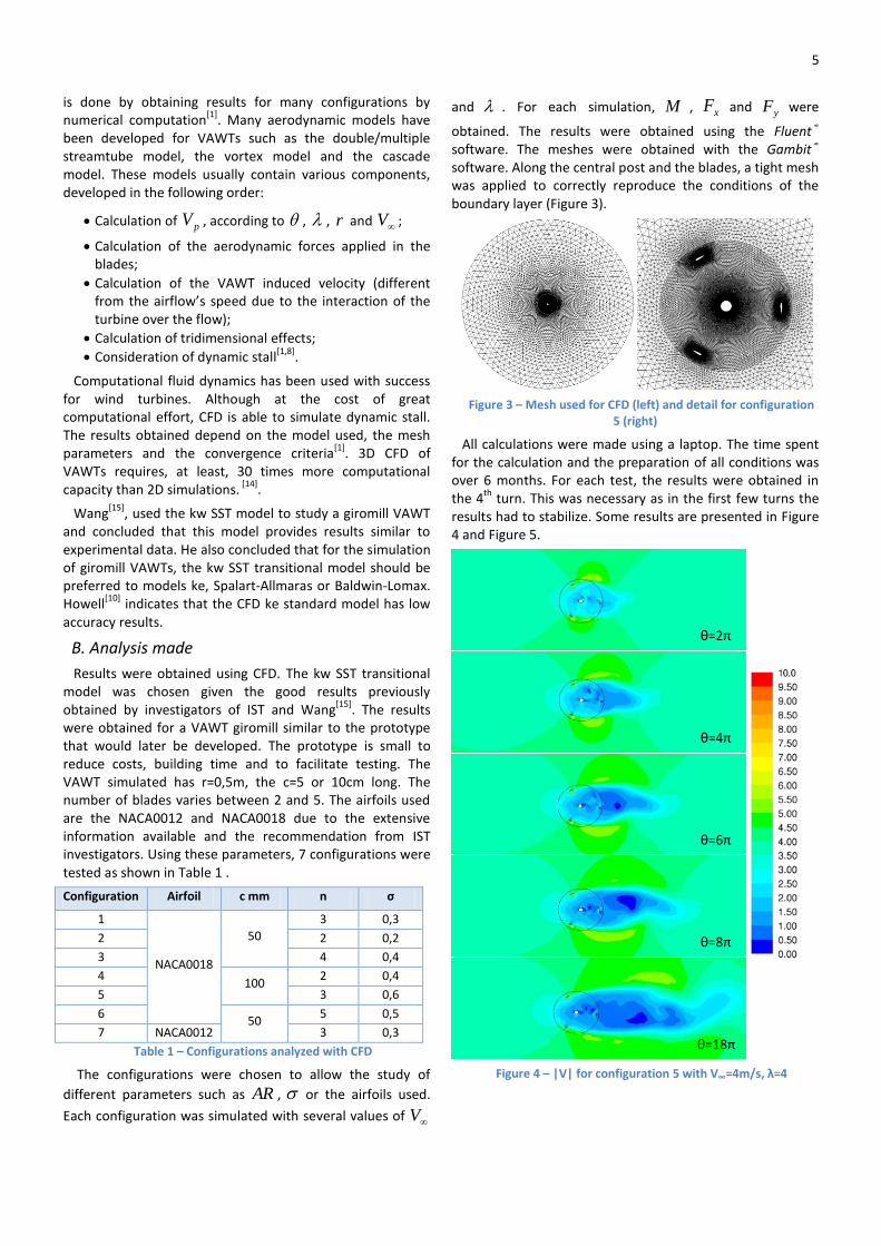
obtained. The results were obtained using the Fluent® software. The meshes were obtained with the Gambit® software. Along the central post and the blades, a tight mesh was applied to correctly reproduce the conditions of the boundary layer (Figure 3).
Figure 3 – Mesh used for CFD (left) and detail for configuration 5 (right)
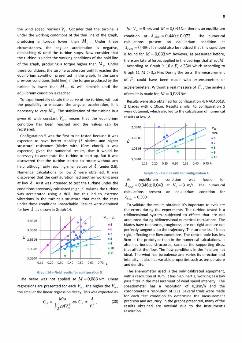
All calculations were made using a laptop. The time spent for the calculation and the preparation of all conditions was over 6 months. For each test, the results were obtained in the 4
th turn. This was necessary as in the first few turns the
results had to stabilize. Some results are presented in Figure 4 and Figure 5.
Figure 4 – |V| for configuration 5 with V∞=4m/s, λ=4
θ=4π
θ=6π
θ=8π
θ=18π
θ=2π
6
Figure 5 - |V| for configuration 5 with V∞=4m/s, λ=4 (detail at 4
th turn)
The results obtained suggest a correct simulation of the physical phenomena involved. There is an alternate vortex formation after the central pole. There’s also, as expected, a
deficit of V inside and after the turbine. This is important
to understand the importance of the development of theoretical models with momentum balance.
Graph 7 shows an example of the results obtained for
configuration 5, where spline curves for 5V m/s and
8V m/s were added to facilitate the visualization.
Graph 7 – CFD results for configuration 5
A compilation of the results obtained is shown in Graph 8.
Not all values of V and were tested for each
configuration, so the value of maxPC presented refers to
the maximum value obtained. As more conditions were
obtained for 5V m/s and 8V m/s, in this range of
values the results presented are expected to have better accuracy.
With these results, we start to evaluate all the configurations with NACA0018 airfoils (all configurations
except number 7). The configurations with 100c mm (4
and 5) yielded better results (about 40%) than the configurations with 50c mm (1, 2, 3 and 6). Even for
configurations with equal , such as configurations 3 and 4,
configuration 4 with higher c has better results. Within the
configurations with 50c mm (1, 2, 3 and 6), the best
result is obtained for 4,0 (configuration 3), existing
configurations with inferior and superior with worst
results. To compare the effect of different airfoils, we can compare configuration 1 (NACA0018) and 7 (NACA0012). Configuration 7, equipped with NACA0012 airfoils yielded better results than configuration 1 (about 30%).
Graph 8 – CPmax according to V∞ for all configurations
Another important evaluation refers to the lateral forces.
Graph 9 shows nF , along for several values of .
Graph 9 - |Fn| according to θ for conf. 5 with V∞=8m/s
nF reaches a certain regularity for high values of . As
the working regime is usually at high (higher PC ), the
more irregular curves may be considered transitional regimes. The other curves, have a sinusoidal form with
variable intensity but approximately constant f . For the
same configuration, similar results are obtained for different
values of V . Graph 10 depicts nF for the other
configurations with 8V m/s and optimum .
The sinusoidal behavior is only presented for configurations with 3 (configurations 5 and 7) and 4 blades (configuration 3). The other configurations have a closely
sinusoidal pattern but with distortions. In these cases, nF
has more than one f , making more difficult the dynamic
-0,15
-0,05
0,05
0,15
0,25
0,35
0 1 2 3 4 5 6
Cp
λ
234567811
V∞ m/s
θ=0x120/5°
θ=2x120/5°
θ=4x120/5°
7
behavior analysis of the turbine. Also, the intensity of nF
varies with each configuration.
Graph 10 - |Fn| according to θ for several configurations with V∞=8 m/s and λoptimum.
V. BUILDING THE VAWT PROTOTYPE
To validate the numerical results previously obtained, a VAWT prototype was designed and built.
A. Bibliographic review
Parashivoiu[1]
refers that the most promising developments in VAWTs are the use of guy cables, truss columns and composite materials. Nowadays, turbine’s blades are usually built with composites with carbon or glass fibers with polyester or epoxy. The interior is filled with sandwich structures composed of PVC, PET or even balsa wood
[16].
The end-of-life disposal of the turbine is also very important. The amount of materials used should be minimum and recyclable (in 2030, near 225000 tons of blades are expected to reach end-of-life). Nowadays only 30% of a fiber reinforced plastic composite can be recycled as new composite. The rest of it can be used as a filling material in construction but most of the blades are reduced in size (a difficult process) and combusted
[17].
For small VAWTs, the best option is the use of easily recyclable plastics (such as PET) and the development of a VAWT easily dismountable and with fewer different materials.
B. Building the prototype
It was expected to build a prototype able to change several parameters such as the number of blades or the blade’s airfoil. To achieve this, a modular design, allowing the use of different modular pieces was developed. The prototype designed was also small and simple to reduce costs, ease testing and allow a fast construction.
The blades were built in the Aerospace department of IST using a hot-wire computer controlled machine. The machine was used to cut the airfoil shape from an insulating foam board. A layer of fiber glass was then applied to the foam blades.
The maximum length of the blades was limited by the hot-wire machine to approximately 1m. The blades were built
with this maximum dimension to increase the AR of the turbine, diminishing the influence of tridimensional effects.
The rest of the prototype was built in a specialized shop (Figure 6).
Figure 6 – Prototype built (without instruments)
It is composed of a central pole attached by two bearings to a wider central pole. Two disks are attached to the external central pole allowing the connection of different sets of arms that support the blades. It is possible to test configurations from 1 to 7 blades. Figure 7 and Figure 8 depict some details.
Figure 7 – Prototype detail
Figure 8 – Prototype detail
VI. TESTING THE PROTOTYPE
A. Bibliographic review
To test the efficiency of a VAWT, it is necessary to control
applying a known M . It is also necessary to measure
V and . The measure of P can be made directly using
dedicated equipment or through M and .
In similar tests, several sensors were used such as pressure sensors, accelerometers or extensometers
[1,2,11]. The use of
various sensors allows for a more detailed set of data, which is important for the complete study of the turbine
0
10
20
30
40
50
60
70
0,00 1,05 2,09 3,14 4,19 5,23 6,28
Fn N
θ rad
Conf.2, λ=4,5
Conf.3, λ=4
Conf.4, λ=3,5
Conf.5, λ=3
Conf.6, λ=3,5
Conf.7, λ=5
8
configuration[19]
. Other interesting tests were made using other techniques such as acoustic emissions or interferometric techniques
[21].
Sheldahl[20]
and Parashivoiu[1]
say that testing a turbine in real conditions is hard due to the variability of wind and the subjection to weather conditions. To avoid this, the use of high sample rate systems is recommended.
B. Tests made
For testing the turbine, a cup anemometer, a speedometer, and a system of weights coupled to a brake, were used. The speedometer was used to obtain . A
bicycle speedometer was used. The sensor was attached to the blades. The value measured was the linear velocity of the blade in km/h.
The brake was used to apply a known M to the turbine. To calibrate the brake, a series of tests were conducted.
Also, it was necessary to calculate the turbine’s M due to effects such as rolling friction. Both were calculated the same way.
First the turbine (without blades) was placed horizontally with a cable rolled in the outer central pole. In the end of the rolled cable, a known weight was tied. Next, the turbine was allowed to rotate freely. Given the effect of the weight, the turbine started to spin, unrolling the cable. The time taken for the weight to cover a certain distance is related to
M in Nm according to
2
2Pr
rt
lIM . (18)
The moment of inertia of the turbine was calculated as
01089918,0I kgm2. The results obtained are presented in
Graph 11.
Graph 11 – Measurement 1 for the brake’s calibration
The M obtained varies with the P used. This was explained by the existence of lateral forces in the bearings that increase the rolling friction. To avoid this, the turbine should be tested without exerting lateral forces on it. This was done by placing the VAWT vertically in its correct position. The VAWT was then accelerated using a drill until a
known constant 0 was obtained. Then the drill was
decoupled from the turbine allowing it to rotate freely.
The time t in s taken for the turbine to stop is related to
M in Nm as
t
IM 0 , (19)
The results obtained are presented in Graph 12.
Graph 12 – Measurement 2 for the brake’s calibration
M obtained is approximately constant. From these results it can be concluded that there is not an important variation
of M with . Using the same test conditions, the brake
was calibrated obtaining the results presented in Graph 13.
Graph 13 – Measurement 3 for the brake’s calibration
It is important to notice that even at high 0 , no
disequilibrium or vibrations were noticed in the turbine’s movement. Under these conditions it was assumed that the main inertial axis was correctly aligned with the turbine’s rotation axis.
It was hard to conciliate the tests with the weather conditions given the season (the tests began in December) and the highly variable weather conditions in the Azores. The prototype should be tested during daylight, without rain with near constant wind. Such conditions rarely occurred.
To test the prototype, a known M was applied to the
turbine using the break. Then when V and stood
approximately constant for at least 20s, the values were registered.
To start-up the turbine, it is usually necessary to reach a minimum . Figure 9 depicts this situation.
Figure 9 – VAWTs working principle
Consider a turbine that respects the curves presented for
two wind speeds, 1V and 2V . Consider 0M the torque
applied in the turbine (considered constant). Consider that
0,00
0,05
0,10
0,15
0,20
0,25
0,00 1,00 2,00 3,00
Torq
ue
Nm
Weight kg
Results
Mean
-0,12
-0,1
-0,08
-0,06
-0,04
0,00 10,00 20,00 30,00 40,00 50,00
Torq
ue
Nm
ω0 rad/s
Results
Mean
-0,35
-0,25
-0,15
-0,05
0 0,5 1
Torq
ue
Nm
Weight kg
Results
Mean
2nd orderlinearregression
y=-0,101x2-0,075x-0,083
9
the wind speed remains 1V . Consider that the turbine is
under the working conditions of the thin line of the graph,
producing a torque lower than 0M . Under these
circumstances, the angular acceleration is negative, diminishing until the turbine stops. Now consider that
the turbine is under the working conditions of the bold line
of the graph, producing a torque higher than 0M . Under
these conditions, the turbine accelerates until it reaches the equilibrium condition presented in the graph. In the same previous conditions (bold line), if the torque produced by the
turbine is lower than 0M , will diminish until the
equilibrium condition is reached.
To experimentally obtain the curve of the turbine, without the possibility to measure the angular acceleration, it is
necessary to vary 0M . The stabilization of the turbine in a
given with constant V , means that the equilibrium
condition has been reached and the values can be registered.
Configuration 5 was the first to be tested because it was expected to have better stability (3 blades) and higher structural resistance (blades with 10cm chord). It was expected, given the numerical results, that it would be necessary to accelerate the turbine to start-up. But it was discovered that the turbine started to rotate without any
help, although only reaching small values of (under 0,6).
Numerical calculations for low were obtained. It was
discovered that the configuration had another working area
at low . As it was intended to test the turbine under the
conditions previously calculated (high values), the turbine
was accelerated using a drill. But this led to extreme vibrations in the turbine’s structure that made the tests under these conditions unreachable. Results were obtained
for low as shown in Graph 14.
Graph 14 – Field results for configuration 5
The brake was not applied so 083,0M Nm. Linear
regressions are presented for each V . The higher the V ,
the smaller the linear regression decay. This was expected as
23
21
V
CAV
MC PP
. (20)
For 8V m/s and 083,0M Nm there is an equilibrium
condition at 073,0440,0 field . The numerical
calculations present an equilibrium condition at
386,0CFD . It should also be noticed that this condition
is found for 083,0M Nm however, as presented before,
there are lateral forces applied in the bearings that affect M. According to Graph 9, 3510 nF N which according to
Graph 11 2,0M Nm. During the tests, the measurement
of nF could have been made with extensometers or
accelerometers. Without a real measure of nF , the analysis
of results is made for 083,0M Nm.
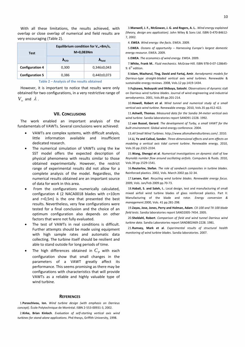
Results were also obtained for configuration 4: NACA0018, 2 blades with c=10cm. Results similar to configuration 5 were obtained, which also led to the calculation of numerical
results at low .
Graph 15 – Field results for configuration 4
An equilibrium condition was found for
043,0346,0 field at 8V m/s. The numerical
calculations present an equilibrium condition for
300,0CFD .
To validate the results obtained it’s important to evaluate the errors during the experiments. The turbine tested is a tridimensional system, subjected to effects that are not accounted during bidimensional numerical calculations. The blades have tolerances, roughness, are not rigid and are not perfectly tangential to the trajectory. The turbine itself is not rigid, affecting the flow conditions. The central pole has less 5cm in the prototype than in the numerical calculations. It also has bonded structures, such as the supporting discs, that affect the flow. The flow conditions in the field are not ideal. The wind has turbulence and varies its direction and intensity. It also has variable properties such as temperature and density.
The anemometer used is the only calibrated equipment, with a resolution of 10m. It has high inertia, working as a low pass filter in the measurement of wind speed intensity. The speedometer has a resolution of 0,1km/h and the chronometer a resolution of 0,1s. Several trials were made for each test condition to determine the measurement precision and accuracy. In the graphs presented, many of the results obtained are overlaid due to the instrument’s resolution.
5,0E-04
1,5E-03
2,5E-03
3,5E-03
4,5E-03
0,10 0,20 0,30 0,40 0,50 0,60 0,70
Cp
λ
5
6
7
8
9
10
11
V∞ m/s
5,0E-04
1,0E-03
1,5E-03
2,0E-03
0,15 0,20 0,25 0,30 0,35 0,40 0,45
Cp
λ
6
7
8
9
10
V∞
m/s
10
With all these limitations, the results achieved, with overlap or close overlap of numerical and field results are very encouraging (Table 2).
Test
Equilibrium condition for V∞=8m/s,
M=0,083Nm
λCFD λfield
Configuration 4 0,300 0,346±0,043
Configuration 5 0,386 0,440±0,073
Table 2 – Analysis of the results obtained
However, it is important to notice that results were only obtained for two configurations, in a very restrictive range of
V and .
VII. CONCLUSIONS
The work enabled an important analysis of the fundamentals of VAWTs. Several conclusions were achieved:
VAWTs are complex systems, with difficult analysis, little information available and insufficient dedicated research.
The numerical simulation of VAWTs using the kw SST model offers the expected description of physical phenomena with results similar to those obtained experimentally. However, the restrict range of experimental results did not allow for a complete analysis of the model. Regardless, the numerical results obtained are an important source of data for work in this area.
From the configurations numerically calculated, configuration 4 (2 NACA0018 blades with c=10cm and r=0,5m) is the one that presented the best results. Nevertheless, very few configurations were tested for a final conclusion and the choice of an optimum configuration also depends on other factors that were not fully evaluated.
The test of VAWTs in real conditions is difficult. Further attempts should be made using equipment with high sample rates and automatic data collecting. The turbine itself should be resilient and able to stand outside for long periods of time.
The high differences obtained in PC with each
configuration show that small changes in the parameters of a VAWT greatly affect its performance. This seems promising as there may be configurations with characteristics that will provide VAWTs as a reliable and highly valuable type of wind turbine.
REFERENCES 1.Paraschivou, Ion. Wind turbine design (with emphasis on Darrieus
concept). École Polytechnique de Montréal. ISBN 2-553-00931-3, 2002.
2.Kirke, Brian Kinloch. Evaluation of self-starting vertical axis wind
turbines for stand-alone applications. Phd thesys, Griffith University, 1998.
3.Manwell, J. F., McGowan, J. G. and Rogers, A. L.. Wind energy explained
(theory, design ans application). John Wiley & Sons Ltd. ISBN 0-470-84612-
7, 2002.
4. EWEA. Wind energy: the facts. EWEA. 2009.
5.EWEA. Oceans of opportunity – Harnessing Europe’s largest domestic
energy resource. EWEA. 2009.
6.EWEA. The economics of wind energy. EWEA. 2009.
7.White, Frank M.. Fluid mechanics. McGraw-Hill. ISBN 978-0-07-128645-
9. 6th edition.
8.Islam, Mazharul, Ting, David and Fartaj, Amir. Aerodynamic models for